Meter Data Managementand Analysis

for Electric Vehicle Charging Infrastructures

Bakkalaureatsarbeit

zur Erlangung des akademischen Grades

Bachelor of Science

im Rahmen des Studiums

Software & Information Engineering

eingereicht von

Bernhard NickelMatrikelnummer 0925384

an derFakultät für Informatik der Technischen Universität Wien

Betreuung: Ao.Univ.-Prof. Dr. Wolfgang KastnerMitwirkung: Dipl.-Ing. Markus Jung

Wien, TT.MM.JJJJ(Unterschrift Verfasserin) (Unterschrift Betreuung)

Technische Universität WienA-1040 Wien � Karlsplatz 13 � Tel. +43-1-58801-0 � www.tuwien.ac.at

Meter Data Managementand Analysis

for Electric Vehicle Charging Infrastructures

Bachelor’s Thesis

submitted in partial fulfillment of the requirements for the degree of

Bachelor of Science

in

Software & Information Engineering

by

Bernhard NickelRegistration Number 0925384

to the Faculty of Informaticsat the Vienna University of Technology

Advisor: Ao.Univ.-Prof. Dr. Wolfgang KastnerAssistance: Dipl.-Ing. Markus Jung

Vienna, TT.MM.JJJJ(Signature of Author) (Signature of Advisor)

Technische Universität WienA-1040 Wien � Karlsplatz 13 � Tel. +43-1-58801-0 � www.tuwien.ac.at

Erklärung zur Verfassung der Arbeit

Bernhard NickelSteudelgasse 30/42, 1100 Wien

Hiermit erkläre ich, dass ich diese Arbeit selbständig verfasst habe, dass ich die verwende-ten Quellen und Hilfsmittel vollständig angegeben habe und dass ich die Stellen der Arbeit -einschließlich Tabellen, Karten und Abbildungen -, die anderen Werken oder dem Internet imWortlaut oder dem Sinn nach entnommen sind, auf jeden Fall unter Angabe der Quelle als Ent-lehnung kenntlich gemacht habe.

(Ort, Datum) (Unterschrift Verfasserin)

i

Abstract

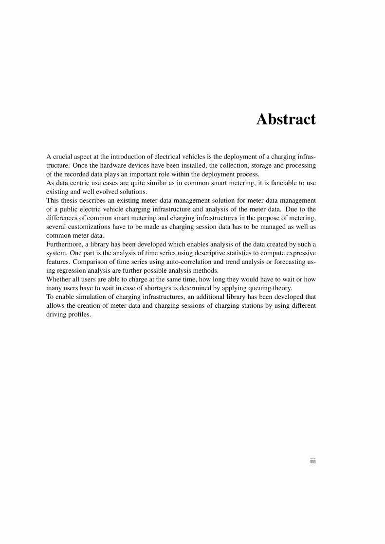
A crucial aspect at the introduction of electrical vehicles is the deployment of a charging infras-tructure. Once the hardware devices have been installed, the collection, storage and processingof the recorded data plays an important role within the deployment process.As data centric use cases are quite similar as in common smart metering, it is fanciable to useexisting and well evolved solutions.This thesis describes an existing meter data management solution for meter data managementof a public electric vehicle charging infrastructure and analysis of the meter data. Due to thedifferences of common smart metering and charging infrastructures in the purpose of metering,several customizations have to be made as charging session data has to be managed as well ascommon meter data.Furthermore, a library has been developed which enables analysis of the data created by such asystem. One part is the analysis of time series using descriptive statistics to compute expressivefeatures. Comparison of time series using auto-correlation and trend analysis or forecasting us-ing regression analysis are further possible analysis methods.Whether all users are able to charge at the same time, how long they would have to wait or howmany users have to wait in case of shortages is determined by applying queuing theory.To enable simulation of charging infrastructures, an additional library has been developed thatallows the creation of meter data and charging sessions of charging stations by using differentdriving profiles.

iii

Kurzfassung

Ein wesentlicher Aspekt bei der Einführung der Elektromobilität ist die Bereitstellung einerLadeinfrastruktur. Dabei spielen neben den eingesetzten Geräten die Erfassung, Speicherung,Verarbeitung und Analyse der anfallenden Daten eine zentrale Rolle.Aufgrund der Ähnlichkeit der Anwendungsfälle zum herkömlichen Smart-Metering im Bereichder Datenerfassung und Verarbeitung und der fortgeschrittenen Entwicklung von Konzepten undLösungen dabei, ist es naheliegend sich an diesen zu orientieren.Inhalt dieser Arbeit ist die Beschreibung des Einsatzes einer bestehenden, ausgereiften Me-ter Data Management Lösung im Umfeld einer öffentlichen Elektromobilitäts-Ladeinfrastrukturund die Analyse der entstehenden Metering Daten. Der Einsatz eines solchen Systems erfordertdiverse Anpassungen der bestehenden Lösung aufgrund der Differenzen zum herkömlichen Me-ter Data Management. So müssen zum Beispiel neben den herkömlichen Zählerdaten Informa-tionen von einzelnen Ladesitzungen verwaltet werden.Weiters wurde im Zuge dieser Arbeit eine Programmbibliothek erstellt, welche die Analyseder in einem solchem System anfallenden Daten erlaubt. Ein Schwerpunkt liegt dabei auf derAnalyse von Zeitreihen, wobei mittels deskriptiver Statistik aussagekräftige Parameter ermittelt,Teilbereiche mittels Autokorrelation miteinander verglichen und Trends bzw. Prognosen mitHilfe der Regressionsanalyse durchgeführt werden können.Ob alle Benutzer/innen ausreichend bedient werden können, wie lange die Wartezeit beträgt undwieviele Benutzer/innen gleichzeitig warten müssen, kann durch Anwendung der Warteschlangen-theorie analysiert werden.Zur Simulation von Ladeinfrastrukturen wurde eine weitere Programmbibliothek erstellt, mitderen Hilfe man Ladesitzungen mit Zählerdaten verschiedener Fahrprofile erzeugen kann.

v

Contents

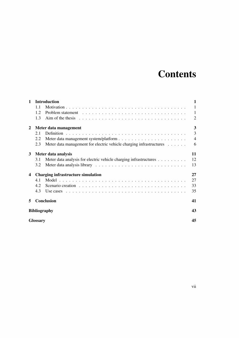
1 Introduction 11.1 Motivation . . . . . . . . . . . . . . . . . . . . . . . . . . . . . . . . . . . . . 11.2 Problem statement . . . . . . . . . . . . . . . . . . . . . . . . . . . . . . . . 11.3 Aim of the thesis . . . . . . . . . . . . . . . . . . . . . . . . . . . . . . . . . 2

2 Meter data management 32.1 Definition . . . . . . . . . . . . . . . . . . . . . . . . . . . . . . . . . . . . . 32.2 Meter data management system/platform . . . . . . . . . . . . . . . . . . . . . 42.3 Meter data management for electric vehicle charging infrastructures . . . . . . 6

3 Meter data analysis 113.1 Meter data analysis for electric vehicle charging infrastructures . . . . . . . . . 123.2 Meter data analysis library . . . . . . . . . . . . . . . . . . . . . . . . . . . . 13

4 Charging infrastructure simulation 274.1 Model . . . . . . . . . . . . . . . . . . . . . . . . . . . . . . . . . . . . . . . 274.2 Scenario creation . . . . . . . . . . . . . . . . . . . . . . . . . . . . . . . . . 334.3 Use cases . . . . . . . . . . . . . . . . . . . . . . . . . . . . . . . . . . . . . 35

5 Conclusion 41

Bibliography 43

Glossary 45

vii

CHAPTER 1Introduction

1.1 Motivation

As many countries are now eager to start reducing their carbon dioxide emissions, electric vehi-cles become a more and more popular topic. There are several different approaches how to dealwith charging processes and periods and one is to provide a public charging infrastructure. It isobvious that the provider of a charging infrastructure has to manage users and assets, chargingsession data and billing procedures. Due to the fact that common asset management, meter datamanagement and billing solutions for smart metering are well evolved and approved it is fancia-ble to integrate them into an overall charging infrastructure solution.To highlight the benefits of the usage of a meter data management solution, applying alreadygained knowledge in data analysis to forecast usage and shortages within the charging infras-tructure is an essential issue.

1.2 Problem statement

There exist many well evolved software solutions for meter data management in common smartmetering. Thus it seems natural to use these solutions for meter data recorded by electric vehiclecharging infrastructures due to the fact that the challenges are quite similar. The major differenceis the additional required effort to manage charging session data associated with different usersand charging points. In common smart metering, metering systems in general just create periodicrecords of the consumption data and a meter is associated with only one customer over the longterm. A public charging infrastructure metering system additionally provides information ofthe start, end, consumption and user of a charging session. To enable the management of thisinformation, an existing meter data management solution has to be customized and / or extendedat several different sites.Computional data analysis is a powerful approach to acquire further information of the collecteddata. To gain useful knowledge, it is necessary to decide what kind of knowledge is valuable

1

and how the data gets analyzed. Which statistical methods will be used and how is it possible toimplement and integrate them into a meter data management system is another important point.To support the decision making process of which data and knowledge is valuable a simulationof a charging infrastructure’s meter data is required.

1.3 Aim of the thesis

Within the scope of this thesis an extension / a customization of an existing meter data manage-ment solution has been designed. The extension consists of an interface (adapter) for a charginginfrastructure head-end system, additional database tables for the storage of session data and anexport interface to a billing system.Furthermore, to enable data analysis, a Java based analysis library has been developed whichcontains mathematical methods for data estimation, derivation, aggregation and statistical meth-ods like auto-correlation or linear regression. As charging processes can be considered as queu-ing processes, queuing analysis by applying queuing theory is also part of the library.To enable ordinary testing of these statistical methods a Java based simulation library that allowscreation of various scenarios has been developed.

2

CHAPTER 2Meter data management

2.1 Definition

As there is no standard definition what meter data management is, it is necessary to define theterm to create a better understanding.

GTM Research separates meter data management into different subcategories where two ofthem do not conflict to other definitions: [1]

• “Meter Data Repository (MDR) – is the database for permanent storage of advanced meterdata, plus the programs and procedures used to process meter data into billing determi-nants so that customer information systems (CIS) can bill time-of-use data. The MDRreceives, validates and stores advanced meter data for billing and other purposes.”

• “Meter Data Management (MDM) is an integration architecture that provides the commu-nication and data management services for sharing and circulating meter data for buildingnew applications and for enhancing existing applications. MDM is a set of enterprise dataservices. A robust MDM platform provides the environment for building service-orientedarchitectures (SOA) for low-cost integration and rapid deployment of new capabilities.”

The definition of advanced metering infrastructure (AMI) is an area of conflict. GTM Re-search defines AMI as a part of meter data management.

“Advanced Metering Infrastructure (AMI) - in this report, we refer to smartmeters as advanced meters. ‘Advanced metering infrastructure’ is used as an en-compassing term for both advanced meters and the supporting field networks thatcontrol and manage meters, including communications from the meter to the widearea network (WAN), which is usually located at the sub-station. Communicationsand services that connect AMI to MDR are considered part of the broader MDMplatform.” [1]

3

Gartner Inc. as opposed to this, defines meter data management as a part of AMI.

“AMI is a composite technology – involving meters (smart meters), communi-cation links and MDM – that spans IT and operational technology (OT) domains,and it supports all components of the meter data life cycle.” [2]

Furthermore, Gartner Inc. defines meter data management as follows:

“MDM products are the IT components of the AMI responsible for cleansing,calculating, and providing data persistency and the dissemination of energy con-sumption data, which can originate from a variety of sources.” [2]

If advanced metering infrastructure is mentioned in the course of this thesis the definition ofGTM Research is applicable.The term meter data management within the scope of this thesis is compliant to definition ofGartner Inc. .

There is also a difference between AMI and automatic meter reading (AMR). Where AMRis used just for collecting meter data requiring unidirectional communication, AMI is also usedfor remote control of smart meters.

2.2 Meter data management system/platform

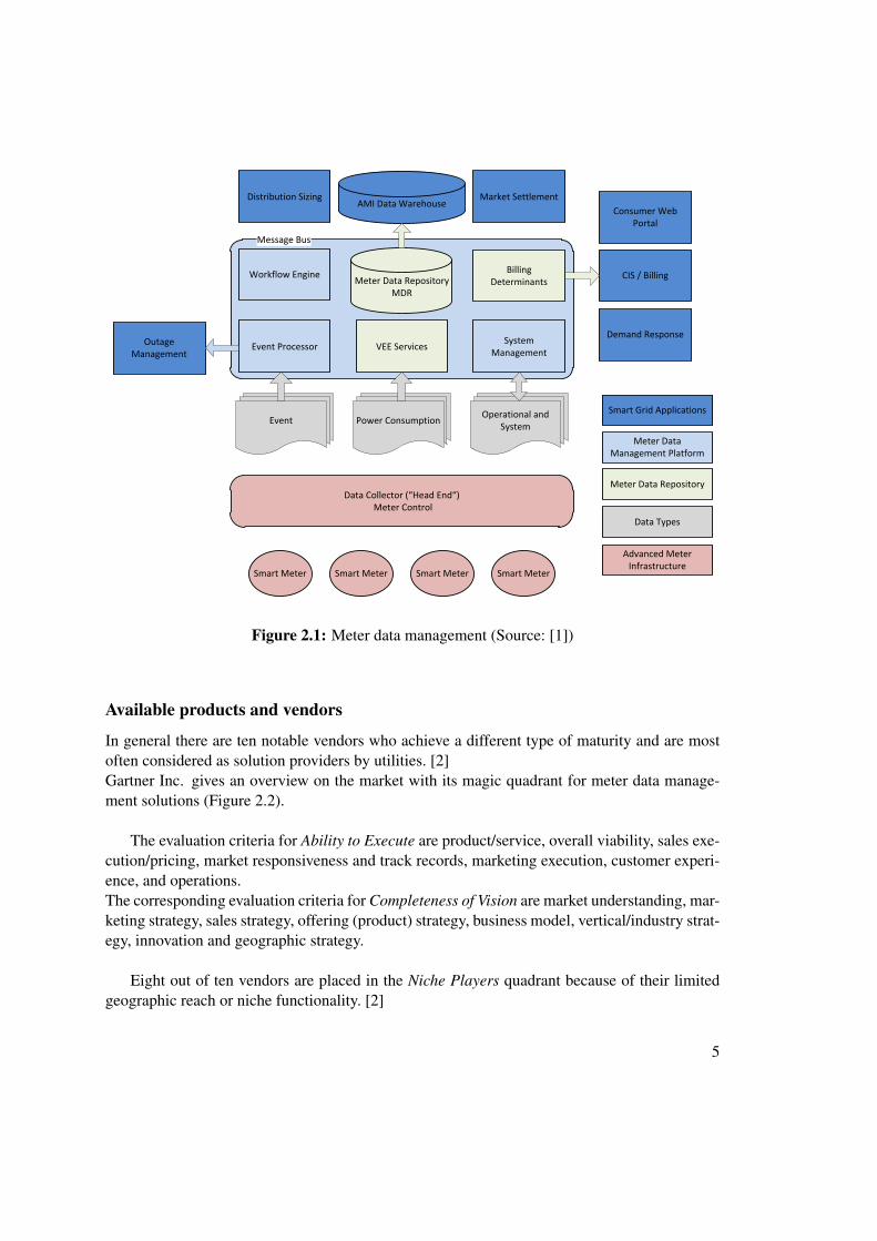
A meter data management system/platform (MDMS) is a set of different software componentsthat enable the processing, storage and forwarding of data created by an advanced metering in-frastructure (Figure 2.1).The head end system (a server application which communicates with the AMI’s components) ofthe AMI sends collected data to the MDMS. As there is no standardized communication proto-col, another integration layer (sometimes called Data Collector) is necessary.Once the MDMS received the data, it performs several validations, estimates missing datarecords and saves it to the database. [1]To assure interoperability, the MDMS has to provide interfaces for all types of collected data.

Requirements

The following requirements are crucial for MDMS: [1]

• Performance and scalability to ensure processability of a huge amount of data

• Reliability and uptime as the processing of meter data is a business critical service ofutilities

• Backup and recovery to prevent data loss

• Security and data privacy to fulfill all directives set by regulators

4

Message Bus

Meter Data RepositoryMDR

VEE ServicesEvent ProcessorSystem

Management

AMI Data WarehouseDistribution Sizing Market Settlement

Workflow Engine CIS / Billing

Consumer Web Portal

Demand ResponseOutage

Management

Event Power ConsumptionOperational and

System

Data Collector (“Head End“) Meter Control

Smart Meter Smart Meter Smart Meter Smart Meter

Billing Determinants

Smart Grid Applications

Meter Data Management Platform

Meter Data Repository

Data Types

Advanced Meter Infrastructure

Figure 2.1: Meter data management (Source: [1])

Available products and vendors

In general there are ten notable vendors who achieve a different type of maturity and are mostoften considered as solution providers by utilities. [2]Gartner Inc. gives an overview on the market with its magic quadrant for meter data manage-ment solutions (Figure 2.2).

The evaluation criteria for Ability to Execute are product/service, overall viability, sales exe-cution/pricing, market responsiveness and track records, marketing execution, customer experi-ence, and operations.The corresponding evaluation criteria for Completeness of Vision are market understanding, mar-keting strategy, sales strategy, offering (product) strategy, business model, vertical/industry strat-egy, innovation and geographic strategy.

Eight out of ten vendors are placed in the Niche Players quadrant because of their limitedgeographic reach or niche functionality. [2]

5

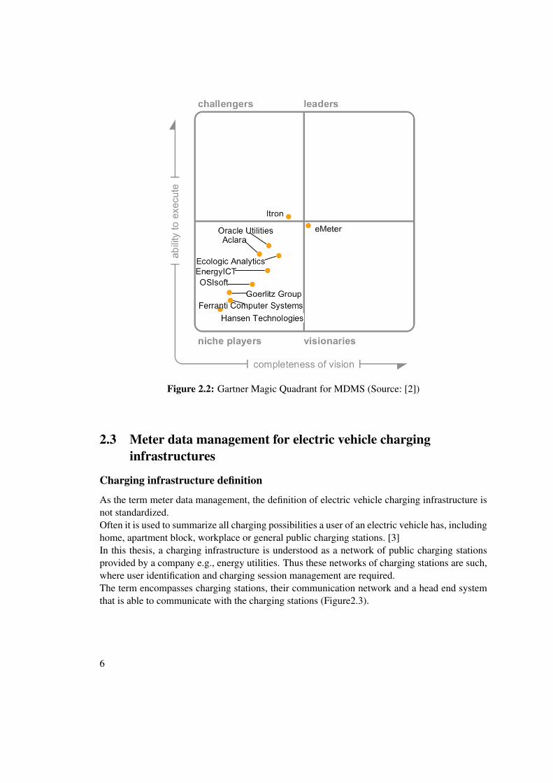
Figure 2.2: Gartner Magic Quadrant for MDMS (Source: [2])

2.3 Meter data management for electric vehicle charginginfrastructures

Charging infrastructure definition

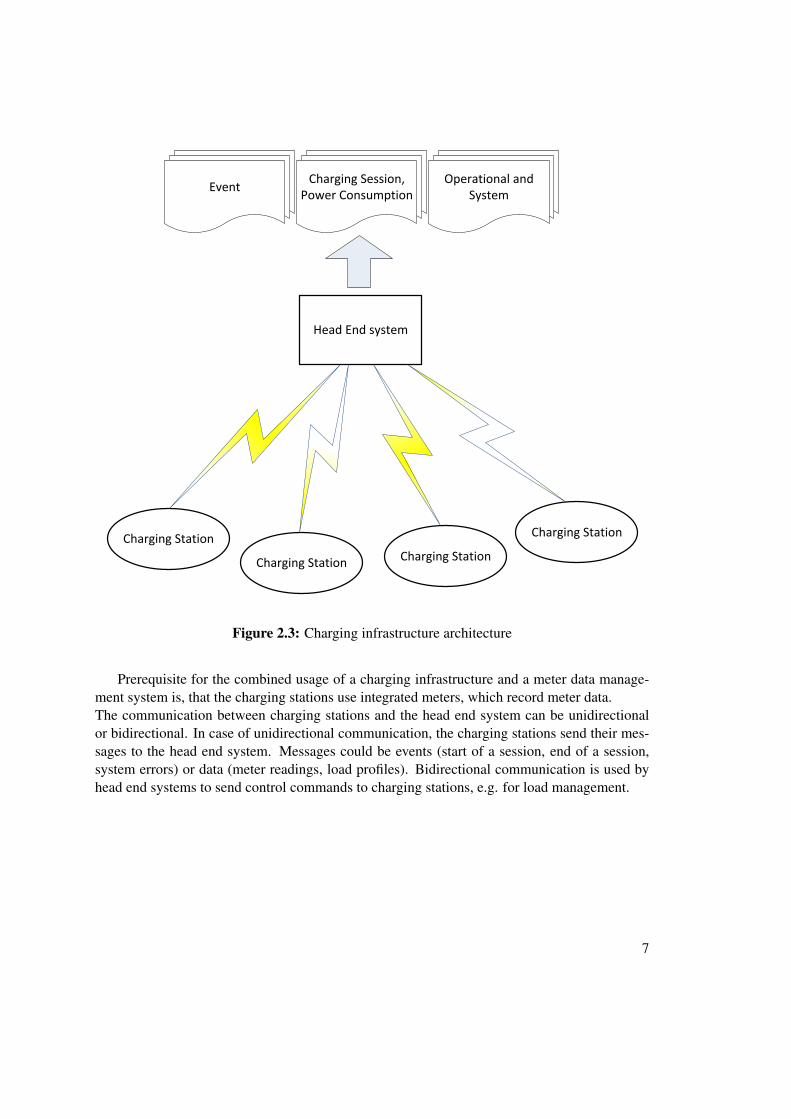
As the term meter data management, the definition of electric vehicle charging infrastructure isnot standardized.Often it is used to summarize all charging possibilities a user of an electric vehicle has, includinghome, apartment block, workplace or general public charging stations. [3]In this thesis, a charging infrastructure is understood as a network of public charging stationsprovided by a company e.g., energy utilities. Thus these networks of charging stations are such,where user identification and charging session management are required.The term encompasses charging stations, their communication network and a head end systemthat is able to communicate with the charging stations (Figure2.3).

6

Charging Station

Charging Station Charging Station

Charging Station

Head End system

EventCharging Session,

Power ConsumptionOperational and

System

Figure 2.3: Charging infrastructure architecture

Prerequisite for the combined usage of a charging infrastructure and a meter data manage-ment system is, that the charging stations use integrated meters, which record meter data.The communication between charging stations and the head end system can be unidirectionalor bidirectional. In case of unidirectional communication, the charging stations send their mes-sages to the head end system. Messages could be events (start of a session, end of a session,system errors) or data (meter readings, load profiles). Bidirectional communication is used byhead end systems to send control commands to charging stations, e.g. for load management.

7

Differentiation to common meter data management

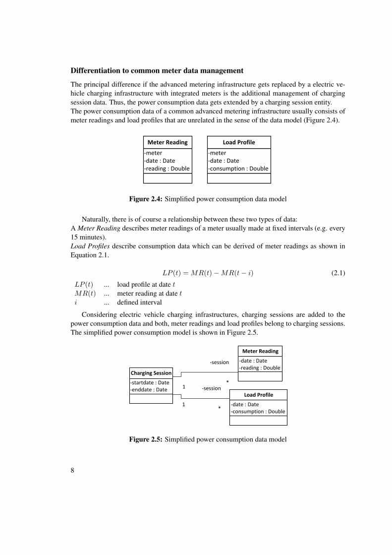
The principal difference if the advanced metering infrastructure gets replaced by a electric ve-hicle charging infrastructure with integrated meters is the additional management of chargingsession data. Thus, the power consumption data gets extended by a charging session entity.The power consumption data of a common advanced metering infrastructure usually consists ofmeter readings and load profiles that are unrelated in the sense of the data model (Figure 2.4).

-meter-date : Date-reading : Double

Meter Reading

-meter-date : Date-consumption : Double

Load Profile

Figure 2.4: Simplified power consumption data model

Naturally, there is of course a relationship between these two types of data:A Meter Reading describes meter readings of a meter usually made at fixed intervals (e.g. every15 minutes).Load Profiles describe consumption data which can be derived of meter readings as shown inEquation 2.1.

LP (t) = MR(t)−MR(t− i) (2.1)

LP (t) ... load profile at date tMR(t) ... meter reading at date ti ... defined interval

Considering electric vehicle charging infrastructures, charging sessions are added to thepower consumption data and both, meter readings and load profiles belong to charging sessions.The simplified power consumption model is shown in Figure 2.5.

-startdate : Date-enddate : Date

Charging Session

-date : Date-reading : Double

Meter Reading

-date : Date-consumption : Double

Load Profile

1

-session

*

1

-session

*

Figure 2.5: Simplified power consumption data model

8

A Charging Session describes a charging process where the startdate is the date once acar starts charging at a charging station. The start_meter_reading is the meter reading of thecharging station’s integrated meter. The enddate and end_meter_reading are the date and meterreading by the time the charging process is finished.

Customization and extension

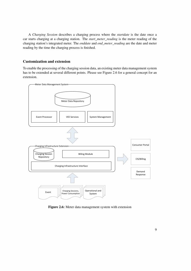
To enable the processing of the charging session data, an existing meter data management systemhas to be extended at several different points. Please see Figure 2.6 for a general concept for anextension.

Meter Data Management System

Meter Data Repository

Event Processor VEE Services System Management

Charging Infrastructure Extension

Charging Session Repository

Charging Infrastructure Interface

Billing Module

CIS/Billing

Charging Sessions,Power Consumption

EventOperational and

System

Demand Response

Consumer Portal

Figure 2.6: Meter data management system with extension

9

To store session data, a charging session data repository is required as the storage of suchdata is not provided by existing solutions.Furthermore, the charging infrastructure interface must be able to store session data in the charg-ing session repository and forward the meter data such as meter readings to the underlyingMDMS.To enable billing or data export to other third-party systems, the extension must also providean export module that merges the data of the meter data repository with the charging sessiondata. The export module of the MDMS just allows access to the meter data of the meter datarepository.

10

CHAPTER 3Meter data analysis

The major purpose of data analysis is to get a better understanding of some data’s characteristics.To achieve this goal a set of methods like descriptive statistics, time series techniques, linearregression models or multivariate exploratory techniques are used in order to: [4]

• maximize the innermost knowledge of the data

• reveal underlying structure

• extract import variables

• develop simple models

With this knowledge, the introduction of smart metering in general, independent of the un-derlying purpose, opens new opportunities by providing large amounts of collected meter datathat can be analyzed.

“It is now possible to view and analyze consumption data in new ways for aplethora of business applications, including capacity planning, demand manage-ment, rate design and reducing peak power consumption.” [5]

More concretely, it is possible to answer questions such as: [6]

• “How much excess energy will be available, when to sell it and whether the grid cantransmit it?”

• “When and where equipment downtime and power failures are most likely to occur?”

• “Which customers are most likely to feed energy back to the grid, and under what circum-stances?”

11

• “Which customers are most likely to respond to energy conservation and demand reduc-tion incentives?”

• “How to manage the commitment of larger, traditional plants in a scenario where peaksfrom distributed generation are becoming relevant?”

Considering electric vehicle charging infrastructures, further and different questions andanalysis scenarios arise:

• Are there enough charging stations for all users/customers of the infrastructure?

• Are there peak times in usage?

• Is the charging behavior of the users/customers seasonal?

• How does the load within the infrastructure evolve in the future?

By using meter data analysis it is possible to find answers to these questions.

3.1 Meter data analysis for electric vehicle charginginfrastructures

In respect to the domain model of power consumption data of electric vehicle charging infras-tructures, as shown in Figure 2.5, it is clear that there are two different types of analyzable data.

First, there are Meter Readings and Load Profiles that are simple time series.Second, there are Charging Sessions, which can be considered as time series values in respect ofstart date and end date and their corresponding values, but can also be considered as processesthat are analyzable using queuing theory since an arrival rate and the residence time can be de-termined.

Time series can be analyzed in several different ways. Descriptive statistics can be used tohighlight main features by determining expressive statistical parameters. Correlation analysisallows the detection of pattern, similarities and seasonality. Regression analysis is useful todetermine trends and forecasting. The analysis of multiserver queues allows the calculation ofperformance measures of a queuing system.Combining these techniques, it is possible to gain valuable knowledge of the data collected andstored by a meter data management system.

12

3.2 Meter data analysis library

The Java library that has been developed within this thesis provides methods for the analysis ofboth, time series and queuing data.There are components that support the calculation of statistical parameters and the correlationcoefficient of autocorrelation, to perform linear regression analysis and to calculate differentperformance measures of multiserver queues.To ensure reusability, the library is not directly coupled to the described domain model. Usingdescriptors, it is applicable on every domain model which can be considered as a time series orqueuing processes. As simple integration is a desired goal, descriptors for the usage of annota-tions are provided.

Architecture

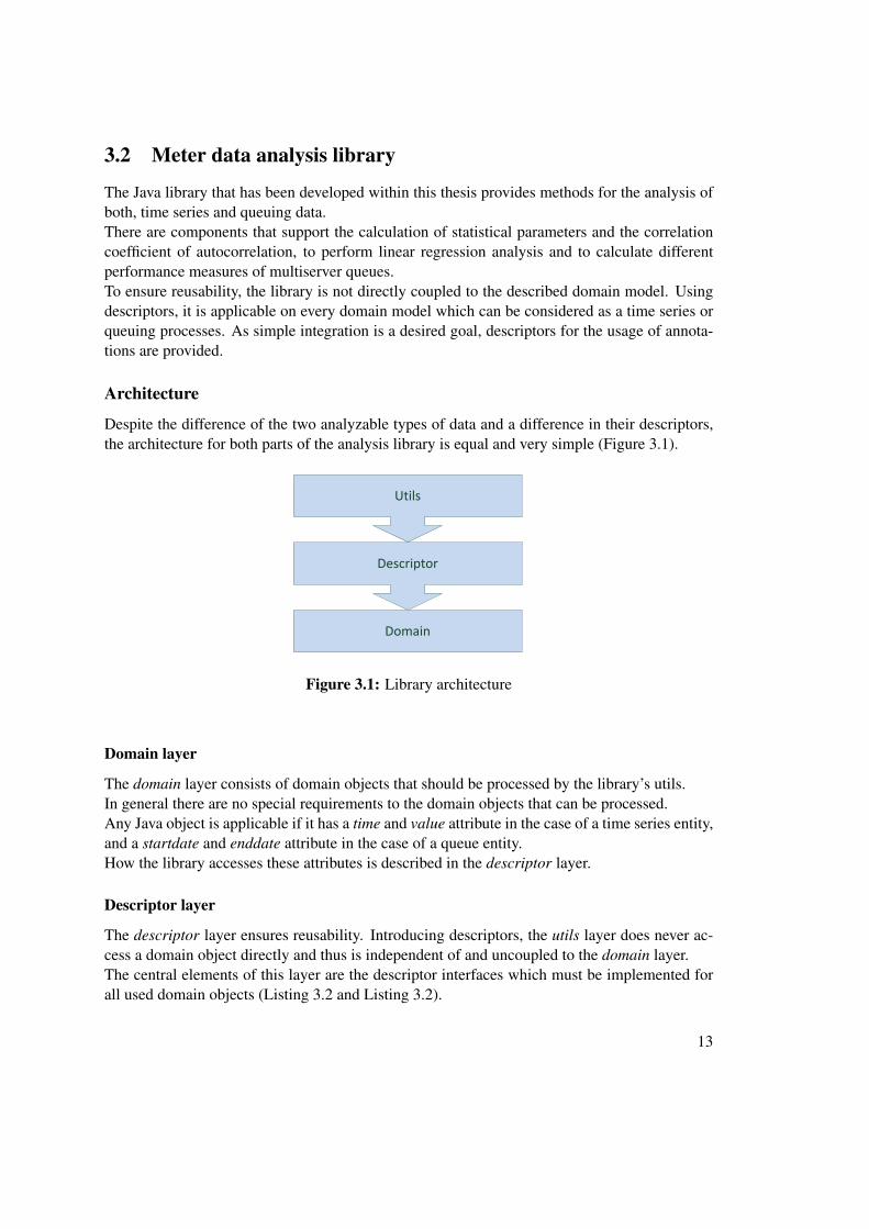
Despite the difference of the two analyzable types of data and a difference in their descriptors,the architecture for both parts of the analysis library is equal and very simple (Figure 3.1).

Utils

Descriptor

Domain

Figure 3.1: Library architecture

Domain layer

The domain layer consists of domain objects that should be processed by the library’s utils.In general there are no special requirements to the domain objects that can be processed.Any Java object is applicable if it has a time and value attribute in the case of a time series entity,and a startdate and enddate attribute in the case of a queue entity.How the library accesses these attributes is described in the descriptor layer.

Descriptor layer

The descriptor layer ensures reusability. Introducing descriptors, the utils layer does never ac-cess a domain object directly and thus is independent of and uncoupled to the domain layer.The central elements of this layer are the descriptor interfaces which must be implemented forall used domain objects (Listing 3.2 and Listing 3.2).

13

public interface TimeSeriesEntityDescriptor<E> {public Date getTime(E e);

public Double getValue(E e);}

Listing 3.1: TimeSeriesEntityDescriptor class

public interface QueueEntityDescriptor<E> {public Date getStartdate(E e);

public Date getEnddate(E e);}

Listing 3.2: QueueEntityDescriptor class

The generic types of the interfaces are naturally the types of the domain objects they de-scribe.

Utils layer

The utils layer provides the functionality to perform the analytical calculations and is providedas a library. As already mentioned, utils access the attributes required for the calculations usingdescriptors. Thus each util must have a reference to its appropriate descriptor (Listing 3.2 andListing 3.2).

public abstract class AbstractTimeSeriesUtil<E> {

protected TimeSeriesEntityDescriptor<E> descriptor;

protected Date getTime(E e) {return descriptor.getTime(e);

}

protected Double getValue(E e) {return descriptor.getValue(e);

}

Listing 3.3: AbstractTimeSeriesUtil class

14

public abstract class AbstractQueueUtil<E> {

protected QueueEntityDescriptor<E> descriptor;

protected Date getStartdate(E e) {return descriptor.getStartdate(e);

}

protected Date getEnddate(E e) {return descriptor.getEnddate(e);

}

Listing 3.4: AbstractQueueUtil class

Every util class in the library is a subclass of one of the two abstract util classes.As the generic type of the util and the descriptor is the same, the interaction between them istype-safe.

Layer interaction

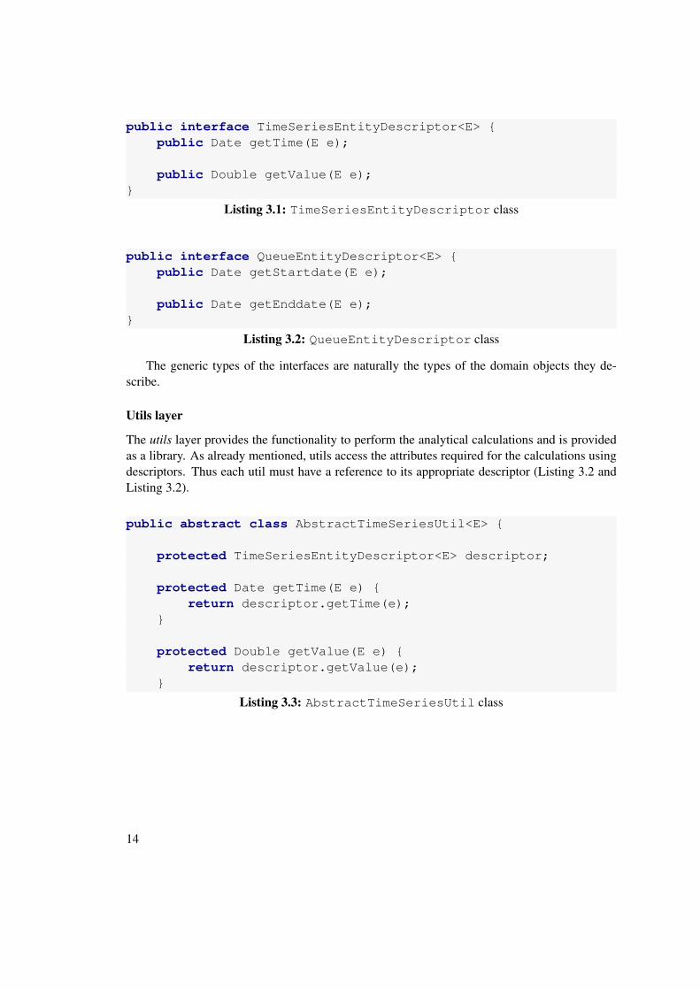
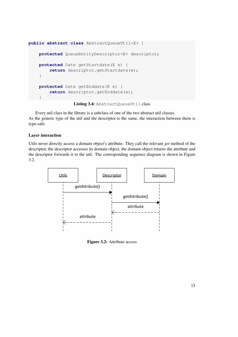
Utils never directly access a domain object’s attribute. They call the relevant get method of thedescriptor, the descriptor accesses its domain object, the domain object returns the attribute andthe descriptor forwards it to the util. The corresponding sequence diagram is shown in Figure3.2.

Utils Descriptor Domain

getAttribute()

getAttribute()

attribute

attribute

Figure 3.2: Attribute access

15

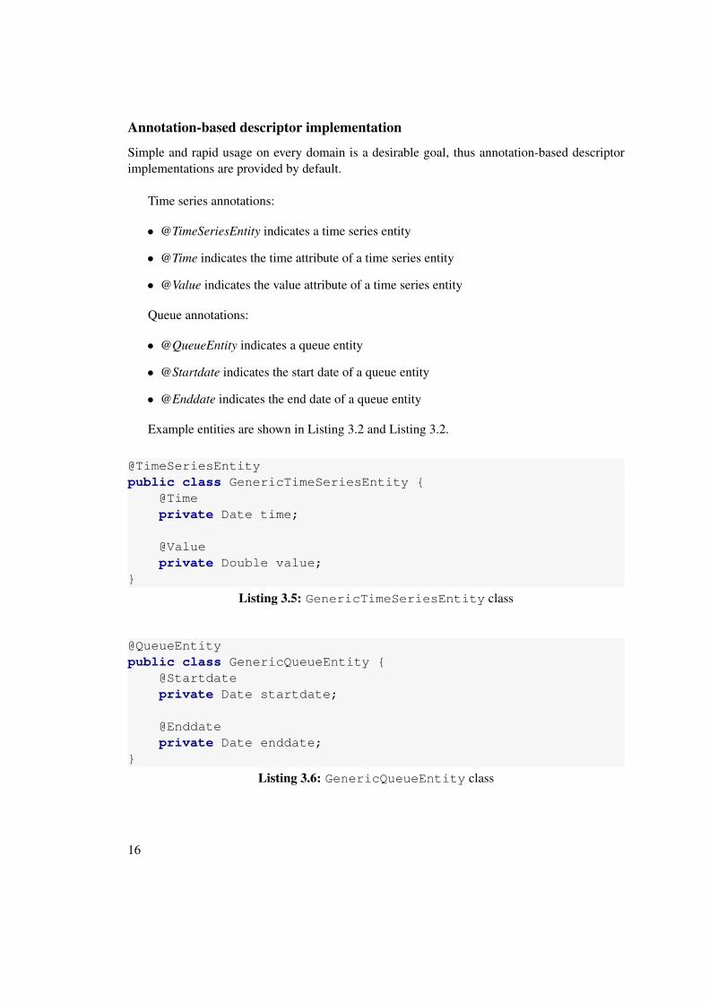
Annotation-based descriptor implementation

Simple and rapid usage on every domain is a desirable goal, thus annotation-based descriptorimplementations are provided by default.

Time series annotations:

• @TimeSeriesEntity indicates a time series entity

• @Time indicates the time attribute of a time series entity

• @Value indicates the value attribute of a time series entity

Queue annotations:

• @QueueEntity indicates a queue entity

• @Startdate indicates the start date of a queue entity

• @Enddate indicates the end date of a queue entity

Example entities are shown in Listing 3.2 and Listing 3.2.

@TimeSeriesEntitypublic class GenericTimeSeriesEntity {

@Timeprivate Date time;

@Valueprivate Double value;

}

Listing 3.5: GenericTimeSeriesEntity class

@QueueEntitypublic class GenericQueueEntity {

@Startdateprivate Date startdate;

@Enddateprivate Date enddate;

}

Listing 3.6: GenericQueueEntity class

16

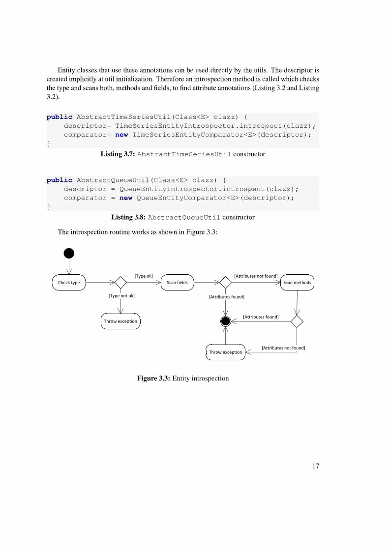
Entity classes that use these annotations can be used directly by the utils. The descriptor iscreated implicitly at util initialization. Therefore an introspection method is called which checksthe type and scans both, methods and fields, to find attribute annotations (Listing 3.2 and Listing3.2).

public AbstractTimeSeriesUtil(Class<E> clazz) {descriptor= TimeSeriesEntityIntrospector.introspect(clazz);comparator= new TimeSeriesEntityComparator<E>(descriptor);

}

Listing 3.7: AbstractTimeSeriesUtil constructor

public AbstractQueueUtil(Class<E> clazz) {descriptor = QueueEntityIntrospector.introspect(clazz);comparator = new QueueEntityComparator<E>(descriptor);

}

Listing 3.8: AbstractQueueUtil constructor

The introspection routine works as shown in Figure 3.3:

Check type Scan fields

Throw exception

Scan methods

Throw exception

[Type ok]

[Type not ok] [Attributes found]

[Attributes not found]

[Attributes found]

[Attributes not found]

Figure 3.3: Entity introspection

17

Time series analysis

Time series analysis is a major purpose of the library, independent whether meter data or othertime series get analysed. A time series is a sequence of collected data that follows a specificorder, denoted by Equation 3.1 [4].

(Xt, t ∈ T ) (3.1)

Where T ⊂ R refers to time. [4]Now it is clear that both, meter readings and load profiles are time series.

The analysis of time series is based on the assumption that the values are taken at equallyspaced time intervals [4]. In the case of power consumption data is gathered typically at 15-minute or hourly intervals. [5]

Time series analysis is separated in two parts. First, data preparation methods are providedto estimate, insert, aggregate or partition data. The second part contains the actual analyticalmethods.

Data preparation

Data preparation is crucial to enable the extraction of useful knowledge of the data. Thus missingvalues have to be estimated, creation of new features must be possible, aggregation is importantto reduce the calculation effort and sampling/partitioning is very important at time series analysisas seasonality may occur. [4]

Estimation Two different methods of value estimation are provided by the library. Both pro-vide functionality to estimate missing values within a list of values of a given interval.

Linear interpolation A simple, but natural estimation method for the estimation of timesseries items is linear interpolation.

The mathematical computation of a value is given in Equation 3.2.

y(x) = ymin +ymax − ymin

xmax − xmin∗ (x− xmin) (3.2)

To enable estimation by linear interpolation within list of values, the provided util iteratesover all intervals within the time range of the list. If a value is missing, it assumes the nearestpresent neighbors as min and max.

Insertion The library provides another method to estimate values. As for linear interpo-lation estimation, a util for insertion of values that iterates over all fixed intervals is provided.To enhance flexibility, the insertion util expects a insertion function as argument, which can beimplemented by the user of the library (Listing 3.2).

18

public interface InsertionFunction {/*** Creates a new value for the given time

** @param time

* @return

*/public double getValue(Date time,Object... additionalArgs);

}

Listing 3.9: InsertionFunction interface

Derivation Derivation is used to create new features in general. Regarding meter data compu-tation, derivation is a method to create load profiles out of recorded meter readings.

The library provides a method for calculating the backward difference of time series itemsaccording to Equation 3.3

dy(t) = y(t)− y(t− i) (3.3)

dy(t) ... derived time series value at date ty(t) ... time series value at date ty(t− i) ... time series value at date t− i where i is the defined interval

Aggregation Aggregation is combining multiple values using a specified aggregate function.This might be used to reduce the amount of data [4] or, in respect of meter data, for instance, tocreate virtual meters by combining multiple meters that share a common characteristic. [5]

For that reason, the library provides functionality to aggregate a list of time series items byiterating over all fixed intervals within a given time range, selecting the associated values andaggregates them using a given aggregate function (Listing 3.2).

public interface AggregationFunction<T> {/*** Aggregates a list of values

** @param values

* @return

*/public double aggregate(List<T> values);

}

Listing 3.10: AggregationFunction interface

19

As summation is a very common aggregate function an implementation is provided whichaggregates correspondent to Equation 3.4.

a(t) =∑

t−i≤tv<t

v(tv) (3.4)

a(t) ... aggregated value for date tv(tv) ... time series value at date tvi ... defined fixed interval

The code snippet for the aggregation is shown in Listing 3.2.

for (long time = startTime; time <= endTime; time += interval){while (index < values.size() && getTime(values.get(index)).

getTime() < time) {aggregationValues.add(values.get(index++));

}aggregatedValues.add(factory.create(new Date(time),

aggregationFunction.aggregate(aggregationValues)));aggregationValues.clear();

}

Listing 3.11: Aggregation snippet

Partitioning Partitioning is important as seasonality may occur over a long term.To compare potential seasons like hours, days, weeks or months, it is necessary to provide apossibility to divide a longer term time series into these parts.The library provides a method for partitioning a time series in parts using a given interval (Listing3.2).

for (long time = startTime; time <= endTime; time += interval){List<E> partition = new ArrayList<E>();

while (index < values.size() && getTime(values.get(index)).getTime() < time) {partition.add(values.get(index++));

}partitions.add(partition);

}

Listing 3.12: Partitioning snippet

20

Analysis

Once the data is prepared, it is possible to perform statistical analysis. Three different types ofanalysis can be performed:

• Descriptive statistics to highlight main features of a sample

• Correlation analysis to detect patterns and seasonality. As the analyzable data is timeseries data, auto-correlation is the concrete form.

• Regression analysis to detect trends and forecasting

Descriptive statistics is used to highlight main features of a sample by calculating differentparameters. The library provides a ParameterUtil that enables the calculation of the followingsample features:

Arithmetic mean The arithmetic mean x of a sample x1, ..., xn is defined by Equation3.5.

x =1

n

n∑i=1

xi (3.5)

Variance The variance of a sample is a measure of how far the sample is spread out (Equa-tion 3.6).

σ2 =1

n

n∑i=1

(xi − x)2 (3.6)

x ... arithmetic mean

Standard deviation As variance (Equation 3.6, standard deviation is a measure of how farthe sample is spread out (Equation 3.7). It is the more meaningful measure since its unit is equalto unit of the sample.

σ =√σ2 (3.7)

21

Covariance Covariance is a measure of how two samples change together (Equation 3.8).[4]

Cov(X,Y ) =1

n

n∑i=1

(xi − x) ∗ (yi − y) (3.8)

x ... arithmetic mean of sample Xy ... arithmetic mean of sample Y

A particular form of the covariance is the auto-covariance, which is a measure of how asample changes to a time-shifted sample of an equal source (Equation 3.9).

γ(t1, t2) =1

n

n∑i=1

(t1i − t1) ∗ (t2i − t2) (3.9)

t1 ... arithmetic mean of sample t1t2 ... arithmetic mean of sample t2

Auto-correlation Auto-correlation is a measure of the similarity of two time-series samplesof the same source. It is used to find patterns and thus enables the detection of seasonality.Its correlation coefficient is defined by Equation 3.10.

ρ(t1, t2) =γ(t1, t2)

σt1 ∗ σt2(3.10)

σt1 ... standard deviation of t1σt2 ... standard deviation of t2γ(t1, t2) ... auto-covariance of t1 and t2

This function gives a value 1 ≥ ρ(t1, t2) ≥ −1 :

1 ... perfect linear correlation of t1 and t20 ... no linear correlation of t1 and t2−1 ... inverted linear correlation of t1 and t2

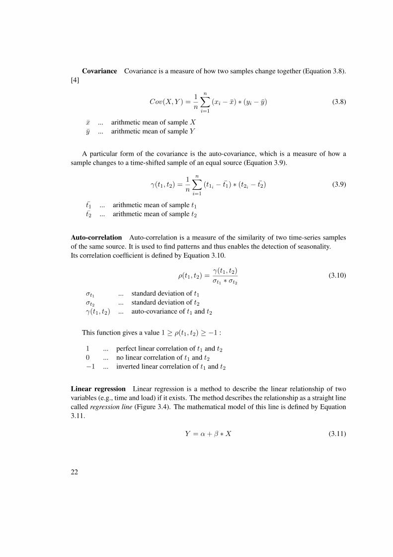
Linear regression Linear regression is a method to describe the linear relationship of twovariables (e.g., time and load) if it exists. The method describes the relationship as a straight linecalled regression line (Figure 3.4). The mathematical model of this line is defined by Equation3.11.

Y = α+ β ∗X (3.11)

22

α and β are parameters which can be calculated using Equation 3.12 and Equation 3.13:

β =

∑ni=1 (xi − x) ∗ (yi − y)∑n

i=1 (xi − x)2(3.12)

The calculation of the parameters is called least square fitting using vertical offsets. [4]

α = y − β ∗ x (3.13)

x ... arithmetic mean of sample Xy ... arithmetic mean of sample Y

Figure 3.4: Linear regression [4]

Queuing analysis

Queuing analysis is the analysis of queues using queuing theory by applying different queuingmodels.

Queues and queuing theory are defined as follows:

“A queue is a special kind of list in which elements may only be removed fromthe bottom by a pop action or added to the top using a push action.” [7]

Queuing theory is “the study of the waiting times, lengths, and other propertiesof queues.” [8]

Other properties would be the number of items in the system, number of items waiting to beserved, their means and standard deviations and traffic intensity. [9]

A typical singleserver queuing system is shown in Figure 3.5.Considering electric vehicle charging infrastructures, a charging station would be a server

and users/drivers items.

23

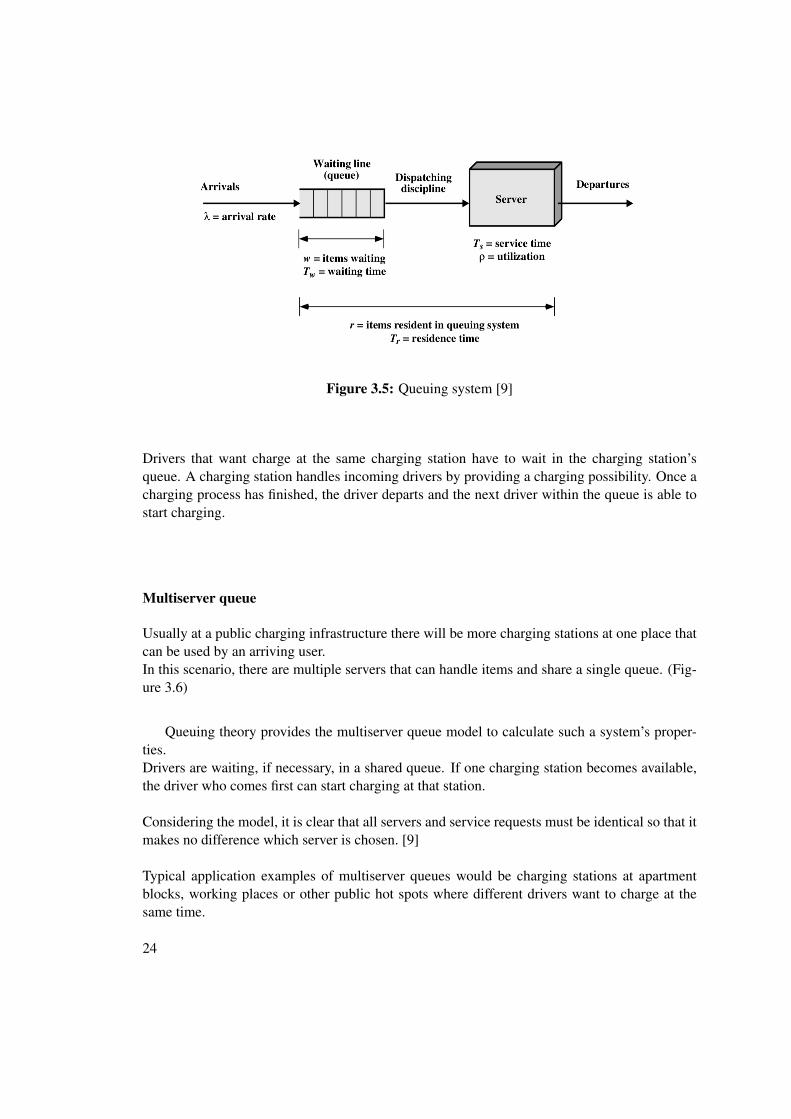
Figure 3.5: Queuing system [9]

Drivers that want charge at the same charging station have to wait in the charging station’squeue. A charging station handles incoming drivers by providing a charging possibility. Once acharging process has finished, the driver departs and the next driver within the queue is able tostart charging.

Multiserver queue

Usually at a public charging infrastructure there will be more charging stations at one place thatcan be used by an arriving user.In this scenario, there are multiple servers that can handle items and share a single queue. (Fig-ure 3.6)

Queuing theory provides the multiserver queue model to calculate such a system’s proper-ties.Drivers are waiting, if necessary, in a shared queue. If one charging station becomes available,the driver who comes first can start charging at that station.

Considering the model, it is clear that all servers and service requests must be identical so that itmakes no difference which server is chosen. [9]

Typical application examples of multiserver queues would be charging stations at apartmentblocks, working places or other public hot spots where different drivers want to charge at thesame time.

24

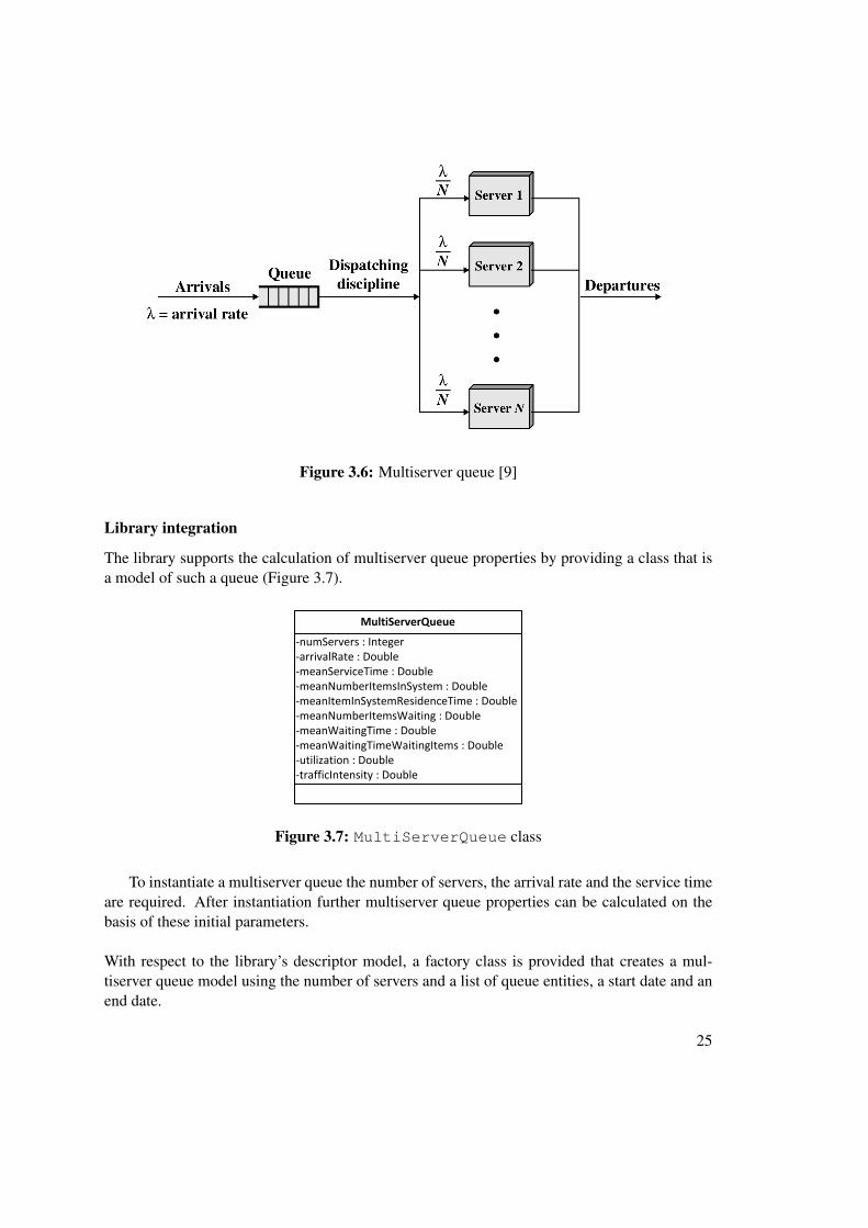
Figure 3.6: Multiserver queue [9]

Library integration

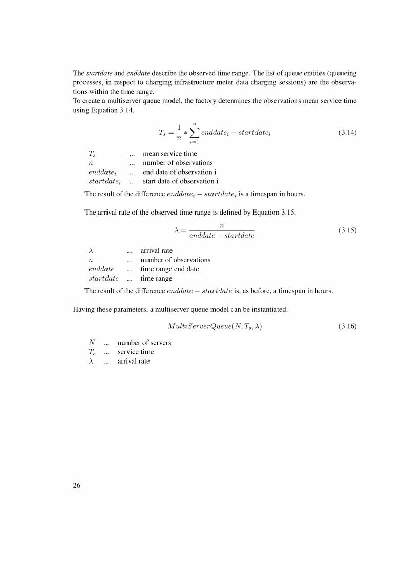
The library supports the calculation of multiserver queue properties by providing a class that isa model of such a queue (Figure 3.7).

MultiServerQueue

-numServers : Integer-arrivalRate : Double-meanServiceTime : Double-meanNumberItemsInSystem : Double-meanItemInSystemResidenceTime : Double-meanNumberItemsWaiting : Double-meanWaitingTime : Double-meanWaitingTimeWaitingItems : Double-utilization : Double-trafficIntensity : Double

Figure 3.7: MultiServerQueue class

To instantiate a multiserver queue the number of servers, the arrival rate and the service timeare required. After instantiation further multiserver queue properties can be calculated on thebasis of these initial parameters.

With respect to the library’s descriptor model, a factory class is provided that creates a mul-tiserver queue model using the number of servers and a list of queue entities, a start date and anend date.

25

The startdate and enddate describe the observed time range. The list of queue entities (queueingprocesses, in respect to charging infrastructure meter data charging sessions) are the observa-tions within the time range.To create a multiserver queue model, the factory determines the observations mean service timeusing Equation 3.14.

Ts =1

n∗

n∑i=1

enddatei − startdatei (3.14)

Ts ... mean service timen ... number of observationsenddatei ... end date of observation istartdatei ... start date of observation i

The result of the difference enddatei − startdatei is a timespan in hours.

The arrival rate of the observed time range is defined by Equation 3.15.

λ =n

enddate− startdate(3.15)

λ ... arrival raten ... number of observationsenddate ... time range end datestartdate ... time range

The result of the difference enddate− startdate is, as before, a timespan in hours.

Having these parameters, a multiserver queue model can be instantiated.

MultiServerQueue(N,Ts, λ) (3.16)

N ... number of serversTs ... service timeλ ... arrival rate

26

CHAPTER 4Charging infrastructure simulation

The previous chapter gives a short introduction to meter data analysis and described a librarythat provides different methods to analyse different types of data. The application of the pro-vided methods is actually not that simple. To conduct experiments and figure out the right usageof the methods, reasonable meter data is required. Thus it is fanciable to simulate charging in-frastructures if no recorded data is available.

Computer simulation, is a method which simulates a simplified model of an exisiting physi-cal system. By making simulation of charging infrastructures available, the creation of artificalmeter data gets enabled. And thus, simulation of such infrastructures is crucial for the develop-ment of crucial analytics use cases.

4.1 Model

The model of the simulation library is divided into three parts.

• The first part are driving profiles that describe different groups of drivers.

• Second, there are electric vehicles that describe the characteristics of their charging pro-cesses load curve and thus the characteristics of the resulting load profiles as they dependon the vehicle’s battery type.

• The third part is the model of charging points, which allows the simulation of chargingstations.

27

Driving profiles

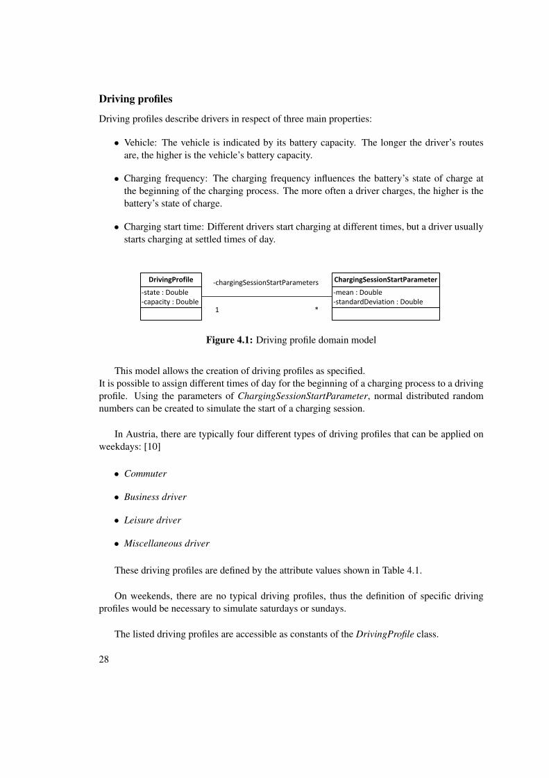
Driving profiles describe drivers in respect of three main properties:

• Vehicle: The vehicle is indicated by its battery capacity. The longer the driver’s routesare, the higher is the vehicle’s battery capacity.

• Charging frequency: The charging frequency influences the battery’s state of charge atthe beginning of the charging process. The more often a driver charges, the higher is thebattery’s state of charge.

• Charging start time: Different drivers start charging at different times, but a driver usuallystarts charging at settled times of day.

DrivingProfile

-state : Double-capacity : Double

ChargingSessionStartParameter

-mean : Double-standardDeviation : Double

1

-chargingSessionStartParameters

*

Figure 4.1: Driving profile domain model

This model allows the creation of driving profiles as specified.It is possible to assign different times of day for the beginning of a charging process to a drivingprofile. Using the parameters of ChargingSessionStartParameter, normal distributed randomnumbers can be created to simulate the start of a charging session.

In Austria, there are typically four different types of driving profiles that can be applied onweekdays: [10]

• Commuter

• Business driver

• Leisure driver

• Miscellaneous driver

These driving profiles are defined by the attribute values shown in Table 4.1.

On weekends, there are no typical driving profiles, thus the definition of specific drivingprofiles would be necessary to simulate saturdays or sundays.

The listed driving profiles are accessible as constants of the DrivingProfile class.

28

Driving profile Capacity Initial state Mean start time Standard deviation

Commuter 20 90%06:30am 1.2h15:30pm 2.7h

Business driver25 55%

08:15am 1.23h11:00am 1.7h16:15pm 1.7h

Miscellaneous driver25 65%

08:15am 1.3h10:15am 1.3h14:15pm 1.25h17:15pm 1.1h

Leisure driver 25 67%11:30am 3.5h18:00pm 1.5h

Table 4.1: Driving profiles [10]

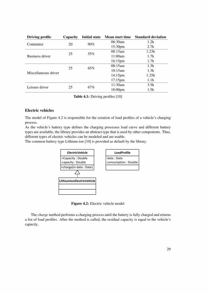
Electric vehicles

The model of Figure 4.2 is responsible for the creation of load profiles of a vehicle’s chargingprocess.As the vehicle’s battery type defines the charging processes load curve and different batterytypes are available, the library provides an abstract type that is used by other components. Thus,different types of electric vehicles can be modeled and are usable.The common battery type Lithium-ion [10] is provided as default by the library.

+charge(in date : Date)

ElectricVehicle

-rCapacity : Double-capacity : Double

LithiumIonElectricVehicle

LoadProfile

-date : Date-consumption : Double

Figure 4.2: Electric vehicle model

The charge method performs a charging process until the battery is fully charged and returnsa list of load profiles. After the method is called, the residual capacity is equal to the vehicle’scapacity.

29

Lithium-ion charging

The charging process of Lithium-ion batteries consists of two phases. [10] Until a specific stateof charge is reached the battery gets charged using constant power. Towards this state of charge,the charging power declines exponential and is defined by Equation 4.1, Equation 4.2 and Equa-tion 4.3.

P = Pconst + es−soc

kl (4.1)

Pconst ... constant charging powers ... state of charge where the charging power begins to declinesoc ... current state of chargekl ... charging breaking current

kl =100− sln Pconst

Pls

(4.2)

Pls =Uls

Un∗ Ils ∗ Ebatt (4.3)

Pls ... charging breaking powerUls ... charging breaking voltageUn ... nominal voltageIls ... charging breaking currentEbatt ... nominal energy

Considering the power source as a typical Austrian power outlet, the parameter values areset as in Table 4.2

To create load profiles in a defined interval, it is necessary to forge a link to the parametertime. The battery capacity is given in kilowatt-hours. The capacity in dependency of the state ofcharge can be calculated using Equation 4.4.

capsoc = 80 ∗ Pconst +

∫ soc

80Pdsoc (4.4)

The unit of capsoc is kilowatt-soc.Because these capacities are in correspondence with each other, the Equation 4.5 can be set

up.

hours

cap=

soc

capsoc(4.5)

Using Equation 4.5, the charging capacity of a period can be calculated.

30

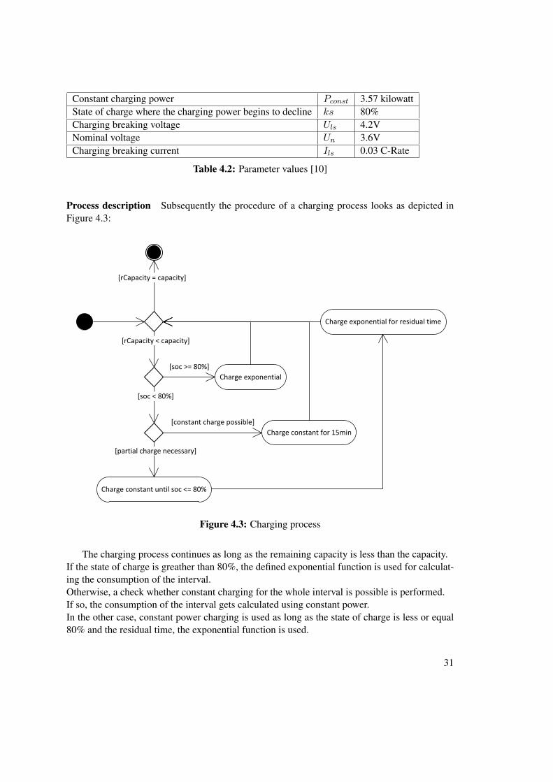
Constant charging power Pconst 3.57 kilowattState of charge where the charging power begins to decline ks 80%Charging breaking voltage Uls 4.2VNominal voltage Un 3.6VCharging breaking current Ils 0.03 C-Rate

Table 4.2: Parameter values [10]

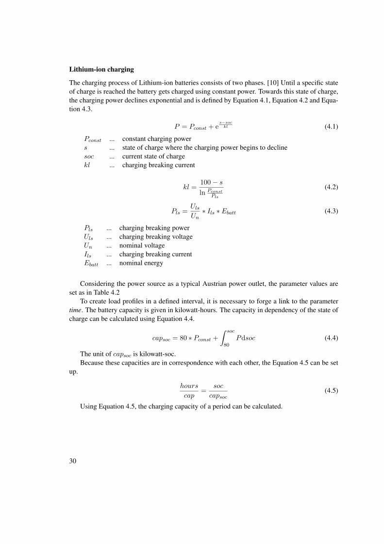
Process description Subsequently the procedure of a charging process looks as depicted inFigure 4.3:

[rCapacity < capacity]

[rCapacity = capacity]

Charge exponential

Charge constant until soc <= 80%

Charge exponential for residual time

Charge constant for 15min

[soc >= 80%]

[soc < 80%]

[partial charge necessary]

[constant charge possible]

Figure 4.3: Charging process

The charging process continues as long as the remaining capacity is less than the capacity.If the state of charge is greather than 80%, the defined exponential function is used for calculat-ing the consumption of the interval.Otherwise, a check whether constant charging for the whole interval is possible is performed.If so, the consumption of the interval gets calculated using constant power.In the other case, constant power charging is used as long as the state of charge is less or equal80% and the residual time, the exponential function is used.

31

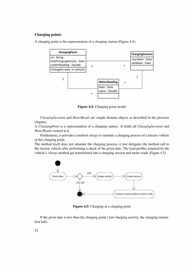
Charging points

A charging point is the representation of a charging station (Figure 4.4).

+charge(in date, in vehicle)

ChargingPoint

-id : String-lastChargingActivity : Date-meterReading : Double

ChargingSession

-startdate : Date-enddate : Date

MeterReading

-date : Date-value : Double

1

*

1

*

1 *

Figure 4.4: Charging point model

ChargingSessions and MeterReads are simple domain objects as described in the previouschapters.A ChargingPoint is a representation of a charging station. It holds all ChargingSessions andMeterReads created at it.

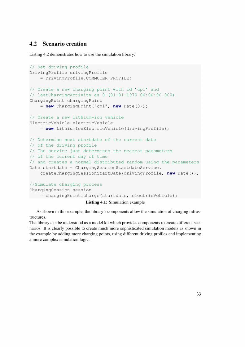
Furthermore, it provides a method charge to simulate a charging process of a electric vehicleat this charging point.The method itself does not simulate the charging process, it just delegates the method call tothe electric vehicle after performing a check of the given date. The load profiles returned by thevehicle’s charge method get transformed into a charging session and meter reads (Figure 4.5).

Check date Charge vehicle Create session

Tranform load profiles to meter reads

[not ok]

[ok]

Figure 4.5: Charging at a charging point

If the given date is less than the charging point’s last charging activity, the charging simula-tion fails.

32

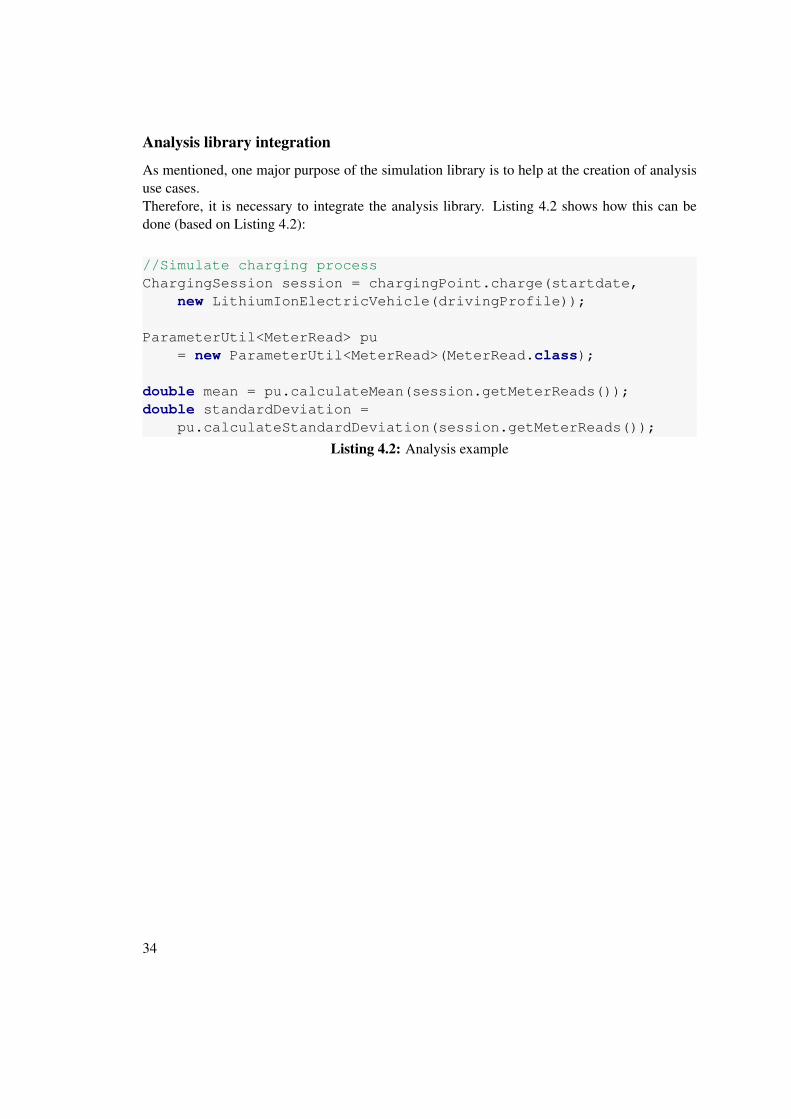
4.2 Scenario creation

Listing 4.2 demonstrates how to use the simulation library:

// Set driving profileDrivingProfile drivingProfile

= DrivingProfile.COMMUTER_PROFILE;

// Create a new charging point with id ’cp1’ and// lastChargingActivity as 0 (01-01-1970 00:00:00.000)ChargingPoint chargingPoint

= new ChargingPoint("cp1", new Date(0));

// Create a new lithium-ion vehicleElectricVehicle electricVehicle

= new LithiumIonElectricVehicle(drivingProfile);

// Determine next startdate of the current date// of the driving profile// The service just determines the nearest parameters// of the current day of time// and creates a normal distributed random using the parametersDate startdate = ChargingSessionStartdateService.

createChargingSessionStartDate(drivingProfile, new Date());

//Simulate charging processChargingSession session

= chargingPoint.charge(startdate, electricVehicle);

Listing 4.1: Simulation example

As shown in this example, the library’s components allow the simulation of charging infras-tructures.The library can be understood as a model kit which provides components to create different sce-narios. It is clearly possible to create much more sophisticated simulation models as shown inthe example by adding more charging points, using different driving profiles and implementinga more complex simulation logic.

33

Analysis library integration

As mentioned, one major purpose of the simulation library is to help at the creation of analysisuse cases.Therefore, it is necessary to integrate the analysis library. Listing 4.2 shows how this can bedone (based on Listing 4.2):

//Simulate charging processChargingSession session = chargingPoint.charge(startdate,

new LithiumIonElectricVehicle(drivingProfile));

ParameterUtil<MeterRead> pu= new ParameterUtil<MeterRead>(MeterRead.class);

double mean = pu.calculateMean(session.getMeterReads());double standardDeviation =

pu.calculateStandardDeviation(session.getMeterReads());

Listing 4.2: Analysis example

34

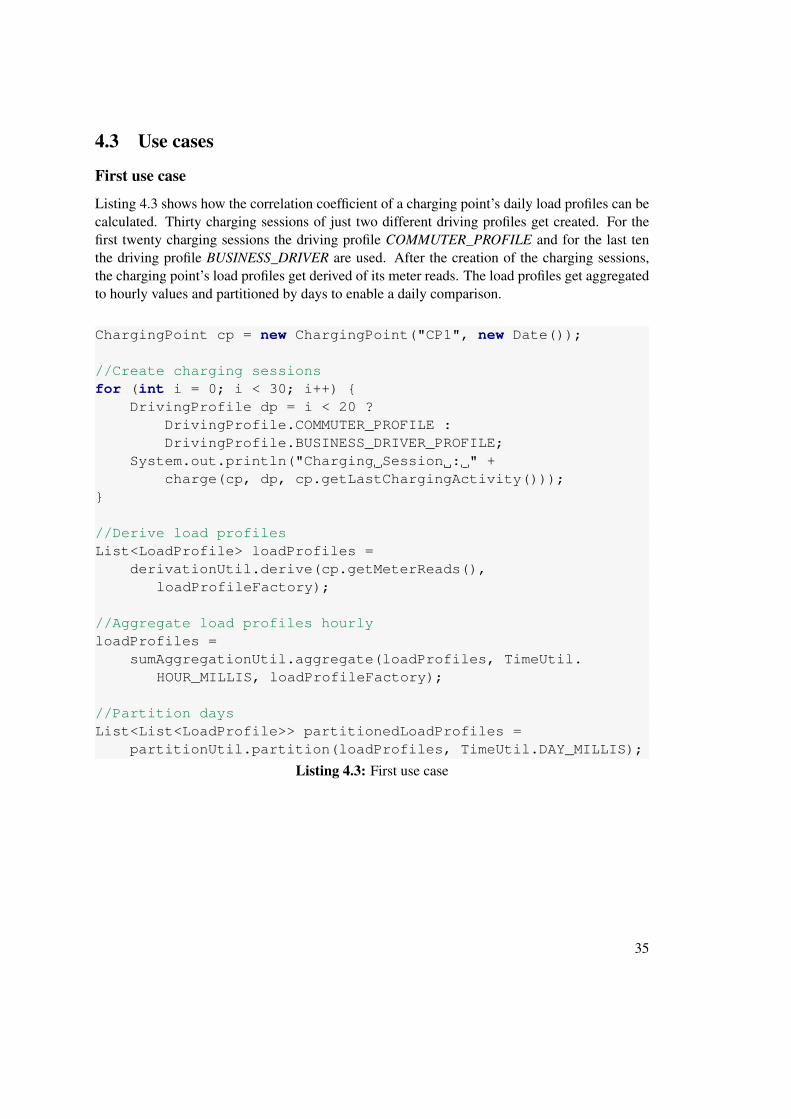
4.3 Use cases

First use case

Listing 4.3 shows how the correlation coefficient of a charging point’s daily load profiles can becalculated. Thirty charging sessions of just two different driving profiles get created. For thefirst twenty charging sessions the driving profile COMMUTER_PROFILE and for the last tenthe driving profile BUSINESS_DRIVER are used. After the creation of the charging sessions,the charging point’s load profiles get derived of its meter reads. The load profiles get aggregatedto hourly values and partitioned by days to enable a daily comparison.

ChargingPoint cp = new ChargingPoint("CP1", new Date());

//Create charging sessionsfor (int i = 0; i < 30; i++) {

DrivingProfile dp = i < 20 ?DrivingProfile.COMMUTER_PROFILE :DrivingProfile.BUSINESS_DRIVER_PROFILE;

System.out.println("Charging Session : " +charge(cp, dp, cp.getLastChargingActivity()));

}

//Derive load profilesList<LoadProfile> loadProfiles =

derivationUtil.derive(cp.getMeterReads(),loadProfileFactory);

//Aggregate load profiles hourlyloadProfiles =

sumAggregationUtil.aggregate(loadProfiles, TimeUtil.HOUR_MILLIS, loadProfileFactory);

//Partition daysList<List<LoadProfile>> partitionedLoadProfiles =

partitionUtil.partition(loadProfiles, TimeUtil.DAY_MILLIS);

Listing 4.3: First use case

35

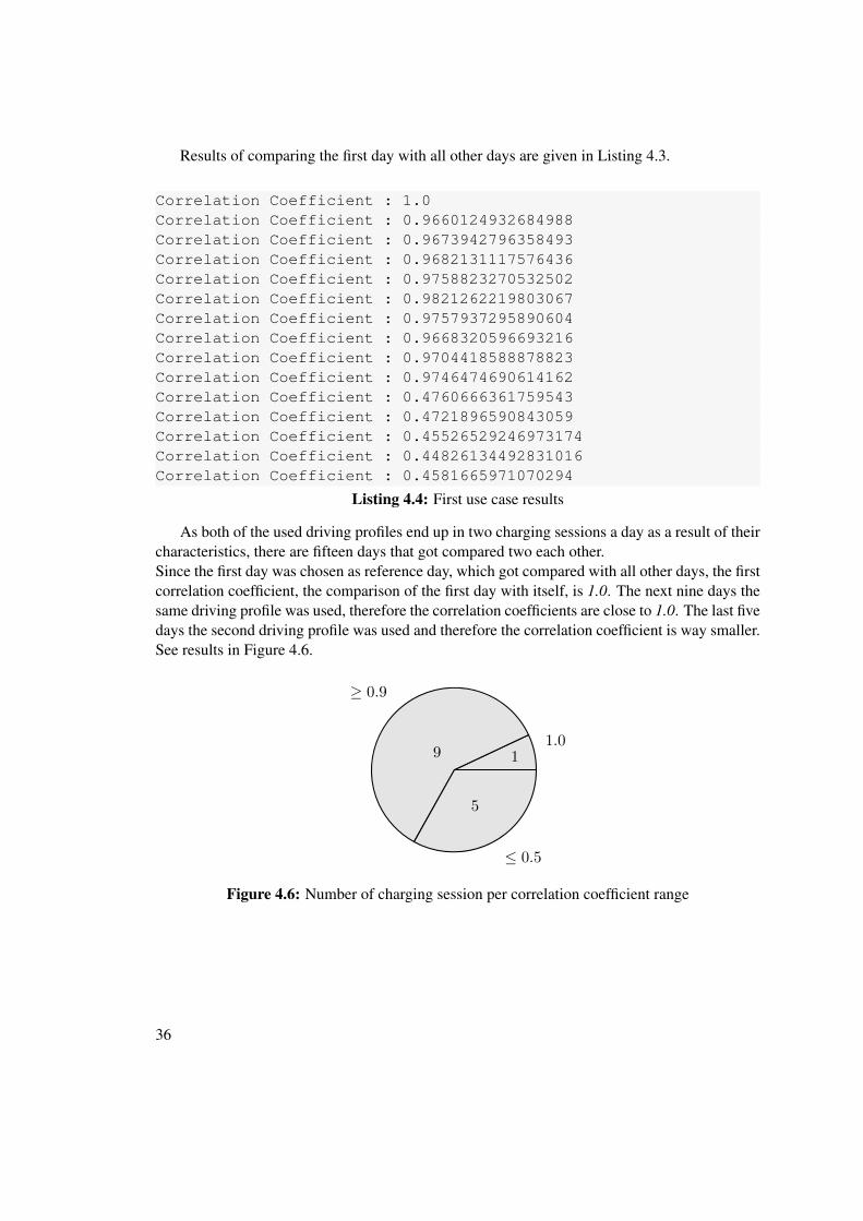
Results of comparing the first day with all other days are given in Listing 4.3.

Correlation Coefficient : 1.0Correlation Coefficient : 0.9660124932684988Correlation Coefficient : 0.9673942796358493Correlation Coefficient : 0.9682131117576436Correlation Coefficient : 0.9758823270532502Correlation Coefficient : 0.9821262219803067Correlation Coefficient : 0.9757937295890604Correlation Coefficient : 0.9668320596693216Correlation Coefficient : 0.9704418588878823Correlation Coefficient : 0.9746474690614162Correlation Coefficient : 0.4760666361759543Correlation Coefficient : 0.4721896590843059Correlation Coefficient : 0.45526529246973174Correlation Coefficient : 0.44826134492831016Correlation Coefficient : 0.4581665971070294

Listing 4.4: First use case results

As both of the used driving profiles end up in two charging sessions a day as a result of theircharacteristics, there are fifteen days that got compared two each other.Since the first day was chosen as reference day, which got compared with all other days, the firstcorrelation coefficient, the comparison of the first day with itself, is 1.0. The next nine days thesame driving profile was used, therefore the correlation coefficients are close to 1.0. The last fivedays the second driving profile was used and therefore the correlation coefficient is way smaller.See results in Figure 4.6.

1.01

≥ 0.9

9

≤ 0.5

5

Figure 4.6: Number of charging session per correlation coefficient range

36

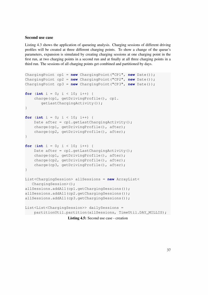
Second use case

Listing 4.3 shows the application of queueing analysis. Charging sessions of different drivingprofiles will be created at three different charging points. To show a change of the queue’sparameters, expansion is simulated by creating charging sessions at one charging point in thefirst run, at two charging points in a second run and at finally at all three charging points in athird run. The sessions of all charging points get combined and partitioned by days.

ChargingPoint cp1 = new ChargingPoint("CP1", new Date());ChargingPoint cp2 = new ChargingPoint("CP2", new Date());ChargingPoint cp3 = new ChargingPoint("CP3", new Date());

for (int i = 0; i < 10; i++) {charge(cp1, getDrivingProfile(), cp1.

getLastChargingActivity());}

for (int i = 0; i < 10; i++) {Date after = cp1.getLastChargingActivity();charge(cp1, getDrivingProfile(), after);charge(cp2, getDrivingProfile(), after);

}

for (int i = 0; i < 10; i++) {Date after = cp1.getLastChargingActivity();charge(cp1, getDrivingProfile(), after);charge(cp2, getDrivingProfile(), after);charge(cp3, getDrivingProfile(), after);

}

List<ChargingSession> allSessions = new ArrayList<ChargingSession>();

allSessions.addAll(cp1.getChargingSessions());allSessions.addAll(cp2.getChargingSessions());allSessions.addAll(cp3.getChargingSessions());

List<List<ChargingSession>> dailySessions =partitionUtil.partition(allSessions, TimeUtil.DAY_MILLIS);

Listing 4.5: Second use case - creation

37

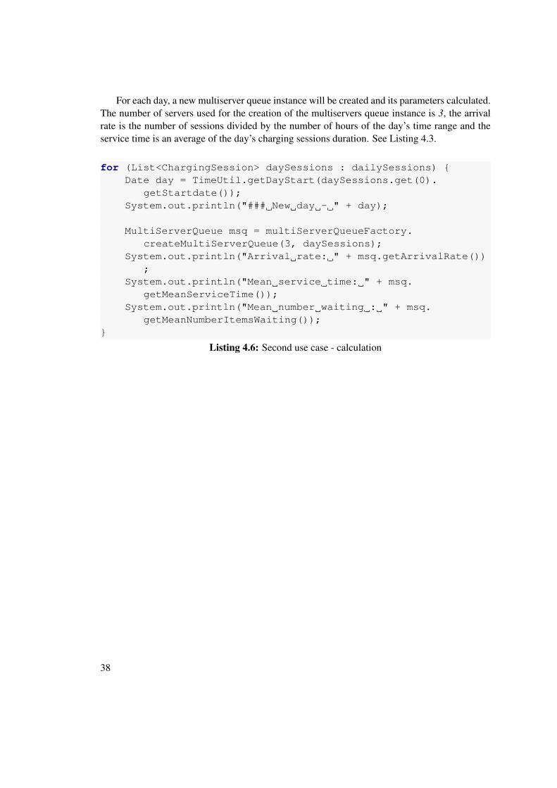
For each day, a new multiserver queue instance will be created and its parameters calculated.The number of servers used for the creation of the multiservers queue instance is 3, the arrivalrate is the number of sessions divided by the number of hours of the day’s time range and theservice time is an average of the day’s charging sessions duration. See Listing 4.3.

for (List<ChargingSession> daySessions : dailySessions) {Date day = TimeUtil.getDayStart(daySessions.get(0).

getStartdate());System.out.println("### New day - " + day);

MultiServerQueue msq = multiServerQueueFactory.createMultiServerQueue(3, daySessions);

System.out.println("Arrival rate: " + msq.getArrivalRate());

System.out.println("Mean service time: " + msq.getMeanServiceTime());

System.out.println("Mean number waiting : " + msq.getMeanNumberItemsWaiting());

}

Listing 4.6: Second use case - calculation

38

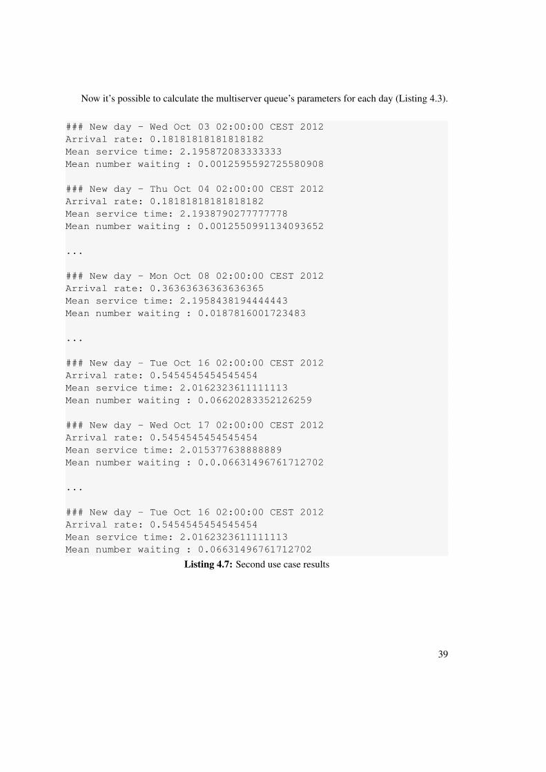
Now it’s possible to calculate the multiserver queue’s parameters for each day (Listing 4.3).

### New day - Wed Oct 03 02:00:00 CEST 2012Arrival rate: 0.18181818181818182Mean service time: 2.195872083333333Mean number waiting : 0.0012595592725580908

### New day - Thu Oct 04 02:00:00 CEST 2012Arrival rate: 0.18181818181818182Mean service time: 2.1938790277777778Mean number waiting : 0.0012550991134093652

...

### New day - Mon Oct 08 02:00:00 CEST 2012Arrival rate: 0.36363636363636365Mean service time: 2.1958438194444443Mean number waiting : 0.0187816001723483

...

### New day - Tue Oct 16 02:00:00 CEST 2012Arrival rate: 0.5454545454545454Mean service time: 2.0162323611111113Mean number waiting : 0.06620283352126259

### New day - Wed Oct 17 02:00:00 CEST 2012Arrival rate: 0.5454545454545454Mean service time: 2.015377638888889Mean number waiting : 0.0.06631496761712702

...

### New day - Tue Oct 16 02:00:00 CEST 2012Arrival rate: 0.5454545454545454Mean service time: 2.0162323611111113Mean number waiting : 0.06631496761712702

Listing 4.7: Second use case results

39

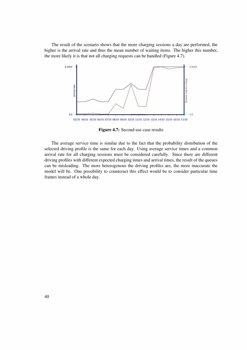
The result of the scenario shows that the more charging sessions a day are performed, thehigher is the arrival rate and thus the mean number of waiting items. The higher this number,the more likely it is that not all charging requests can be handled (Figure 4.7).

Mean

nu

mb

er waitin

g

Arr

ival

rat

e

0.5454 0.0663

04/10 05/10 06/10 07/10 08/10 09/10 10/10 11/10 12/10 13/10 14/10 15/10 16/10 17/1003/10

0.00.0

Figure 4.7: Second use case results

The average service time is similar due to the fact that the probability distribution of theselected driving profile is the same for each day. Using average service times and a commonarrival rate for all charging sessions must be considered carefully. Since there are differentdriving profiles with different expected charging times and arrival times, the result of the queuescan be misleading. The more heterogenous the driving profiles are, the more inaccurate themodel will be. One possibility to counteract this effect would be to consider particular timeframes instead of a whole day.

40

CHAPTER 5Conclusion

Existing meter data management solutions can be used for the management of the meter dataof public electric vehicle charging infrastructures. To enable usage, existing solutions must beextended by a component that handles the management of charging session data. The compo-nent must have a data collection interface which separates charging session data and meter data.Charging session data can only be stored in the component’s charging session repository, whilemeter data must be forwarded to the underlying meter data management system. Furthermore,the component must also provide an export interface where the data is combined again.Meter data analysis is a useful method to gain additional knowledge from the large amounts ofstored data. Thus applying such method is a desirable goal. The meter data analysis library en-ables the application of several analytical methods in an easy way. It is possible to analyze timeseries by computing expressive statistical parameters, applying auto-correlation or performingregression analysis. As charging sessions can be considered as queuing processes, the analysisof charging sessions using queuing theory is also possible.The simulation of real world scenarios is very useful for many purposes as it enables the con-duction of experiments. The simulation library provides models of the most common drivingprofiles and a simulator of a charging station which is able to create realistic meter data. Byusing this library the creation of different models which generate reasonable data is possible.

41

Bibliography

[1] C. Geschickter, The Emergence of Meter Data Management (MDM): A Smart Grid Infor-mation white paper. GTM Research, 2010.

[2] Z. Sumic, Magic Quadrant for Meter Data Management Products. Gartner Industry Re-search, 2010.

[3] VDE Verband der Elektrotechnik Elektronik Informationstechnik e.V.,“http://www.vde.com/de/e-mobility/ladeinfrastruktur/seiten/default.aspx.” Accessed:2012-06-21.

[4] F. Gorunescu, Data Mining,Concepts, Models and Techniques. Springer-Verlag BerlinHeidelberg, 2011.

[5] G. Research, Understanding the Potential of Smart Grid Data Analytics. Greentech MediaInc., eMeter, 2011.

[6] IBM, Managing big data for smart grids and smart meters. IBM Corporation, 2012.

[7] Weisstein, Eric W., Queue. MathWorld–A Wolfram Web Resource.http://mathworld.wolfram.com/Queue.html, 2012.

[8] Weisstein, Eric W., Queuing Theory. MathWorld–A Wolfram Web Resource.http://mathworld.wolfram.com/QueuingTheory.html, 2012.

[9] W. Stallings, Queuing Analysis. WilliamStallings.com, 2000.

[10] M. Litzlbauer, “Erstellung und Modellierung von stochastischen Ladeprofilen mobiler En-ergiespeicher mit MATLAB,” Master’s thesis, Vienna University of Technology, 2009.

43

Glossary

AMI Advanced metering infrastructure. 3–5

IT Information technology. 4

MDM Meter data management. 3, 4

MDMS Meter data management system/platform. 5, 9

MDR Meter data repository. 3, 4

45