Metabolomics data analysis with Bioconductor · Metabolomics? •...
20
Metabolomics data analysis with Bioconductor Johannes Rainer (Eurac Research, Italy) 1 June 12, 2017 @CSAMA2017 1 email: [email protected], github/twitter: jotsetung
Transcript of Metabolomics data analysis with Bioconductor · Metabolomics? •...

Metabolomics data analysis with Bioconductor
Johannes Rainer (Eurac Research, Italy)1
June 12, 2017 @CSAMA2017
1email: [email protected], github/twitter: jotsetung
Talk content
• Very short introduction to metabolomics data analysis.
• Focus on pre-processing of LCMS data.
• Focus on the xcms package (new user interface), but other exist too(e.g. yamss).
Metabolomics?
• Is the large-scale study of small molecules (metabolites) in a system(cell, tissue or organism).
• Metabolites are intermediates and products of cellular processes(metabolism).
• Metabolome?:
• Genome: what can happen.
• Transcriptome: what appears to be happening.
• Proteome: what makes it happen.
• Metabolome: what actually happened. Influenced by genetic andenvironmental factors.

How are we measuring that?
• Nuclear magnetic Resonance (NMR) - not covered here.
• Mass spec (MS)-based metabolomics
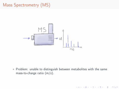
Mass Spectrometry (MS)
• Problem: unable to distinguish between metabolites with the samemass-to-charge ratio (m/z).

Liquid Chromatography Mass Spectrometry (LCMS)
• Combines physical separation via LC with MS for mass analysis.
• Additional time dimension to separate different ions with same m/z.
• LCMS metabolomics: identify peaks in the m/z - rt plane.

LCMS-based metabolomics data pre-processing
• Input: mzML or netCDF files with multiple MS spectra per sample.
• Output: matrix of abundances, rows being features, columnssamples.
• feature: ion with a unique mass-to-charge ratio (m/z) and retentiontime.
• Example: load files from the faahKO data packages, process usingxcms.library(xcms)library(faahKO)library(RColorBrewer)
cdf_files <- dir(system.file("cdf", package = "faahKO"), recursive = TRUE,full.names = TRUE)[c(1, 2, 7, 8)]
## Read the datafaahKO <- readMSData2(cdf_files)
• OnDiskMSnExp: small memory size, loads data on-demand.

LCMS-based metabolomics data pre-processing
• Chromatographic peak detection.
• Sample alignment.
• Correspondence.

LCMS pre-processing: Peak detection
• Goal: Identify chromatographic peaks within slices along mzdimension.
• What type of peaks have to be detected?mzr <- c(241.1, 241.2)chrs <- extractChromatograms(faahKO, mz = mzr, rt = c(3550, 3800))
cols <- brewer.pal(3, "Set1")[c(1, 1, 2, 2)]plotChromatogram(chrs, col = paste0(cols, 80))

LCMS pre-processing: Peak detection
• centWave (Tautenhahn et al. BMC Bioinformatics, 2008):
• Step 1: Detection of regions of interest
• mz-rt regions with low mz-variance.

LCMS pre-processing: Peak detection
• Step 2: Peak detection using continuous wavelet transform (CWT)
• Allows to identify peaks with different widths.
LCMS pre-processing: Peak detection
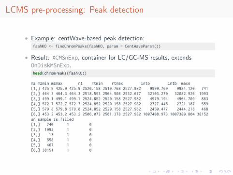
• Example: centWave-based peak detection:faahKO <- findChromPeaks(faahKO, param = CentWaveParam())
• Result: XCMSnExp, container for LC/GC-MS results, extendsOnDiskMSnExp.head(chromPeaks(faahKO))
mz mzmin mzmax rt rtmin rtmax into intb maxo[1,] 425.9 425.9 425.9 2520.158 2510.768 2527.982 9999.769 9984.120 741[2,] 464.3 464.3 464.3 2518.593 2504.508 2532.677 32103.270 32082.926 1993[3,] 499.1 499.1 499.1 2524.852 2520.158 2527.982 4979.194 4904.709 883[4,] 572.7 572.7 572.7 2524.852 2520.158 2527.982 2727.446 2721.187 559[5,] 579.8 579.8 579.8 2524.852 2520.158 2527.982 2450.477 2444.218 468[6,] 453.2 453.2 453.2 2506.073 2501.378 2527.982 1007408.973 1007380.804 38152sn sample is_filled[1,] 740 1 0[2,] 1992 1 0[3,] 13 1 0[4,] 558 1 0[5,] 467 1 0[6,] 38151 1 0

LCMS pre-processing: Alignment
• Goal: Adjust retention time differences/shifts between samples.
• Total ion chromatogram (TIC) representing the sum of intensitiesacross a spectrum.
• Overview of algorithms: (Smith et al. Brief Bioinformatics 2013).
• xcms: peak groups (Smith et. al Anal Chem 2006), obiwarp (Princeet al. Anal Chem, 2006),

LCMS pre-processing: Alignment
• Example: use obiwarp to align samples.faahKO <- adjustRtime(faahKO, param = ObiwarpParam())
• TIC after adjustment:
• Assumptions:
• Samples relatively similar (either similar chromatograms or a set ofcommon metabolites present in all).
• Analyte elution order same in all samples.
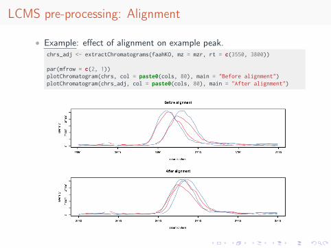
LCMS pre-processing: Alignment
• Example: effect of alignment on example peak.chrs_adj <- extractChromatograms(faahKO, mz = mzr, rt = c(3550, 3800))
par(mfrow = c(2, 1))plotChromatogram(chrs, col = paste0(cols, 80), main = "Before alignment")plotChromatogram(chrs_adj, col = paste0(cols, 80), main = "After alignment")

LCMS pre-processing: Correspondence
• Goal: Group detected chromatographic peaks across samples.
• Peaks that are close in rt (and m/z) are grouped to a feature.
• xcms: peak density method:

LCMS pre-processing: Correspondence
• Example: peak grouping.faahKO <- groupChromPeaks(faahKO, param = PeakDensityParam())
• featureValues: extract values for each feature from each sample.## Access feature intensitieshead(featureValues(faahKO, value = "into"))
ko15.CDF ko16.CDF wt15.CDF wt16.CDFFT0001 6029.945 NA 4586.527 NAFT0002 1144.015 NA 1018.815 NAFT0003 NA 774.576 1275.475 NAFT0004 NA NA 1284.728 1220.7FT0005 2759.095 3872.963 NA NAFT0006 7682.585 3806.080 NA NA
• Fill-in values for missing peaks: fillChromPeaks.

What next? Data normalization
• Adjust within and between batch differences.
• MetNorm RUV for metabolomics (Livera et al. Anal Chem 2015).
• Injection order dependent signal drift (Wehrens et al. Metabolomics2016).
What next? Identification
• Annotate features to metabolites.
• Each metabolite can be represented by multiple features (ionadducts, isotopes).
• Starting point: CAMERA package.
• On-line spectra databases (e.g. MassBank).

Finally. . .
thank you for your attention!
• Hands on in the afternoon labs:
• Proteomics lab.
• Metabolomics lab (pre-processing of LCMS data).