Mach Learn (2012) 87:357–380DOI 10.1007/s10994-012-5286-7

Meta-learning for evolutionary parameter optimizationof classifiers

Matthias Reif · Faisal Shafait · Andreas Dengel

Received: 16 September 2010 / Accepted: 16 March 2012 / Published online: 13 April 2012© The Author(s) 2012

Abstract The performance of most of the classification algorithms on a particular datasetis highly dependent on the learning parameters used for training them. Different approacheslike grid search or genetic algorithms are frequently employed to find suitable parametervalues for a given dataset. Grid search has the advantage of finding more accurate solutionsin general at the cost of higher computation time. Genetic algorithms, on the other hand, areable to find good solutions in less time, but the accuracy of these solutions is usually lowerthan those of grid search.

This paper uses ideas from meta-learning and case-based reasoning to provide good start-ing points to the genetic algorithm. The presented approach reaches the accuracy of gridsearch at a significantly lower computational cost. We performed extensive experiments foroptimizing learning parameters of the Support Vector Machine (SVM) and the RandomForest classifiers on over 100 datasets from UCI and StatLib repositories. For the SVMclassifier, grid search achieved an average accuracy of 81 % and took six hours for training,whereas the standard genetic algorithm obtained 74 % accuracy in close to one hour of train-ing. Our method was able to achieve an average accuracy of 81 % in only about 45 minutes.Similar results were achieved for the Random Forest classifier. Besides a standard geneticalgorithm, we also compared the presented method with three state-of-the-art optimizationalgorithms: Generating Set Search, Dividing Rectangles, and the Covariance Matrix Adap-tation Evolution Strategy. Experimental results show that our method achieved the highestaverage accuracy for both classifiers. Our approach can be particularly useful when trainingclassifiers on large datasets where grid search is not feasible.

Editor: Hendrik Blockeel.

M. Reif (�) · F. Shafait · A. DengelGerman Research Center for Artificial Intelligence, Trippstadter Straße 122, 67663 Kaiserslautern,Germanye-mail: matthias.reif@dfki.de

F. Shafaite-mail: faisal.shafait@dfki.de

A. Dengele-mail: andreas.dengel@dfki.de

358 Mach Learn (2012) 87:357–380

Keywords Meta-learning · Parameter optimization · Genetic algorithm · Feature selection

1 Introduction

In pattern recognition, classifiers are trained on labeled data to produce a function that mapsdata points from the feature space to the label space. This function is used to predict thelabel of a new data point. Typically, classifiers contain several parameters, which influencetheir performance. A typical performance measure is the classification accuracy that is therate of correctly predicted labels. For one single dataset, the optimal parameter setting forthe classifier maximizes the performance on that dataset. The task of finding these optimalparameter values is often called parameter tuning or parameter optimization and is a crucialstep for obtaining good results from most of the classifiers. Parameter tuning has severalaspects, which make it hard in general:

– Parameter settings that result in good performance values for one dataset may not lead togood results for another dataset.

– The parameter values usually depend on each other. It is not sufficient to optimize multipleparameters independently.

– The evaluation of one parameter setting can be already very time-consuming. Most of theclassifiers must be trained from scratch again.

– The search space can be huge due to several facts: (1) A classifier can have many param-eters. (2) The range of the parameters may be large. (3) Real-valued parameters can besensitive to very small changes.

Many deterministic and probabilistic approaches with different complexities and worstcase guarantees have been used for parameter optimization of classifiers. A widely useddeterministic method for parameter optimization is grid search because it is simple and typi-cally delivers good results. However, if the run-time of the optimization is important, it maynot be feasible anymore. A large number of classifier evaluations have to be performed usingthis exhaustive method. Some authors have used more sophisticated deterministic optimiza-tion algorithms such as the Dividing Rectangles (DIRECT) algorithm (Jones et al. 1993) orQuasi-Newton methods (Ayat et al. 2002). However, grid search remains the most widelyused method as long as its computational demands can be met.

For high-dimensional optimization problems or training on large datasets, grid searchbecomes computationally infeasible. In such scenarios, probabilistic optimization methodssuch as genetic algorithms (Goldberg 1989) are usually preferred. For instance, architecture,weights, and learning parameters of artificial neural networks were optimized using suchevolutionary approaches by Yao (1993). The Covariance Matrix Adaptation Evolution Strat-egy (Hansen and Ostermeier 2001) is a modification of standard genetic algorithm that up-dates the covariance matrix used for selecting the next generation. Friedrichs and Igel (2005)used this method to optimize multiple parameters of Support Vector Machines (SVM).Merelo et al. (2001) presented G-LVQ, which uses a genetic algorithm to optimize LearningVector Quantization (Kohonen 1998). Other probabilistic methods have also been used forparameter optimization of classifiers. For example, to optimize parameters of an SVM, Pat-tern Search (Kolda et al. 2003) was used by Momma and Bennett (2002) as well as by Eitrichand Lang (2006), and a gradient descent-based approach was used by Chapelle et al. (2002).

The results achieved using genetic optimization depend on the choice of the start popula-tion (see Sect. 2 for details). It is known that the performance of a genetic algorithm can beincreased if good starting points are used. It was also shown that manually selecting goodstart points for the Nelder-Mead simplex optimization algorithm increases its performance

Mach Learn (2012) 87:357–380 359

(Shafait and Breuel 2011). In this paper, we present an approach that uses experience to findgood start points for the evolutionary parameter optimization of classifiers. The approachuses concepts from meta-learning and adapts them to parameter optimization.

Meta-learning typically tries to predict the applicability of different classification algo-rithms on a dataset, either by predicting only the best algorithm (Bensusan and Giraud-Carrier 2000a; Ali and Smith 2006), predicting a ranking of multiple algorithms (Merz 1995;Berrer et al. 2000; Brazdil et al. 2003), or predicting the performance of algorithms individ-ually (Gama and Brazdil 1995; Sohn 1999; Köpf et al. 2000; Bensusan and Kalousis 2001).More recently, discovering suitable data mining workflows have been investigated by us-ing data mining ontologies (Hilario et al. 2011) and workflow templates (Kietz et al. 2010).Meta-learning has been rarely used for parameter prediction. The only work in this directionuses meta-learning to predict kernel parameters for Support Vector Machines (Soares et al.2004; Soares and Brazdil 2006). A good survey on meta-learning is the paper by Smith-Miles (2008).

The approach presented in this paper uses meta-learning to predict good parameter valuesfor a new dataset. However, instead of directly applying the predicted parameters, they serveas a base for a following optimization step. The random initialization of the genetic algo-rithm is replaced by using these predicted values as start points. Combining the predictionsof meta-learning with a genetic optimization reduces the risks of poor solutions comparedto applying both methods separately. If the meta-learning predicts poor parameter values,the following optimization step is able to correct them. On the other hand, if the geneticalgorithm starts with an already promising solution, its risk of ending up far away from theoptimum will be reduced as well. This is an important aspect because genetic algorithms donot provide any worst case guarantees as grid search does.

For the evaluation of the presented approach, we used two state-of-the-art classifiers:

Support Vector Machine (SVM): SVM (Cortes and Vapnik 1995) is a non-linear maximummargin classifier using a kernel function. A typical kernel function is the radial basis func-tion that contains the parameter γ . The penalty parameter C of SVMs controls the trade-offbetween minimizing the number of wrongly labeled training samples and maximizing themargin. We considered optimization of these two parameters in this work. A more detaileddescription of the SVM classifier including its parameters can be found in Burges (1998).We choose the SVM classifier because it has been very successfully used for a wide rangeof datasets from different domains. Additionally, the training time is rather high comparedto other classifiers. This makes it harder to optimize, because the evaluation of just oneparameter setting can be already very time-consuming.

Random Forest (RF): RF (Breiman 2001) is an ensemble classifier combining random se-lection of features with bagging. Multiple decision trees are created using a random subsetof the attributes. For classification, all trees are applied and make a prediction. The finalclass is determined by a voting scheme among them. RF is also a widely used classifierand contains several parameters. In this work, we optimized five parameters: number oftrees, number of randomly chosen attributes, minimum number of instances for a split,minimum split ratio, and the number of categories for random category split search. Theminimum split ratio defines how balanced a split must be in order to be accepted. The lastparameter determines the maximal number of possible splits of an attribute for performingan exhaustive split search instead of a random split search.

The rest of this paper is structured as follows: first, we give a brief introduction to geneticalgorithms in Sect. 2 and highlight their problems using SVM parameter optimization as anexample. Section 3 describes the methodology of the new approach and Sect. 4 contains anextensive evaluation of it. The conclusion and future work make up the last section.

360 Mach Learn (2012) 87:357–380

2 Genetic algorithms for parameter optimization

Genetic algorithms are a common search strategy and optimization method that are inspiredby biological evolution. A population of individuals evolves over multiple generations. Theindividuals with higher fitness values survive and new individuals are generated by crossing-over and/or mutating existing individuals in the population. This leads to an increase in theaverage fitness of the population over multiple generations.

In optimization, each individual of the population is a candidate solution of the problem.The fitness of the individual is the quality of this solution. The goal is to find a solution withthe highest fitness value. The algorithm works in principle as follows:

– Creation of a random start population of r individuals.– Evaluation of the fitness of all individuals in the population.– Random selection of individuals for next generation according to their fitness. Some

individuals may be doubled whereas individuals with a poor solution will be discarded.– Probabilistic mutation of single individuals.– Probabilistic cross-over by recombining two individuals to create two new individuals.– Stop if the stop criterion is fulfilled. Otherwise, continue with step 2.

As stopping criterion, different rules can be used. For instance, the search can be stopped ifa maximum number of generations were reached or if no better solution was found during adefined number of consecutive generations. The output of the algorithm is usually the bestsolution found during the search.

For parameter optimization of a classifier, a solution is one specific setting of all parame-ters of the classifier that should be optimized. The fitness of the individual is the performanceachieved by the classifier using these parameter values. This means, whenever a solution hasto be evaluated, the concerned classifier has to be trained again. For most classifiers, this isthe most time-consuming part in contrast to the actual classification. If cross-validation isused, even multiple trainings of the classifier are needed for determining the quality of oneparameter setting.

Because genetic algorithms select solutions with higher quality, the search is guided toregions of the search space with more promising solutions. Although the search is not guideddirectly to a local optimum and may not find any better solution over generations, it con-verges to a local optimum in sufficient time with a high probability.

A problem occurs when big parts of the search space consist only of solutions with thesame fitness value. In this case, it is likely that all individuals of a random start populationhave equal fitness values. This is problematic for selecting individuals for the next generationprobabilistically according to their fitness values. If all solutions have the same fitness value,they also have the same selection probability. The search cannot be guided to regions withbetter solutions and randomly moves within the region with equal quality solutions instead.This increases the number of generations needed to find the best solution significantly.

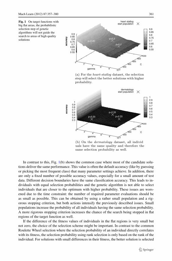
In the worst case, it can miss out the optimum completely and end up far away fromit. One reason for that is a stopping criterion that is often used: the search is stopped ifseveral consecutive generations do not lead to any improvement. This scenario is illustratedin Fig. 1 using the datasets heart-statlog and dermatology from the UCI machine learningrepository (Asuncion and Newman 2007). The plot shows the SVM accuracy values fordifferent combinations of the parameters γ and C. In Fig. 1(a), the three individuals havedifferent selection probabilities due to their different fitness values. The better individualswill be selected more probably and the search will be continued in these more promisingregions.

Mach Learn (2012) 87:357–380 361

Fig. 1 On target functions withbig flat areas, the probabilisticselection step of geneticalgorithms will not guide thesearch to areas of high qualitysolutions

In contrast to this, Fig. 1(b) shows the common case where most of the candidate solu-tions deliver the same performance. This value is often the default accuracy (like by guessingor picking the most frequent class) that many parameter settings achieve. In addition, thereare only a fixed number of possible accuracy values, especially for a small amount of testdata. Different decision boundaries have the same classification accuracy. This leads to in-dividuals with equal selection probabilities and the genetic algorithm is not able to selectindividuals that are closer to the optimum with higher probability. These issues are wors-ened due to the time constraint: the number of required parameter evaluations should beas small as possible. This can be obtained by using a rather small population and a rig-orous stopping criterion, but both actions intensify the previously described issues. Smallpopulations increase the probability of all individuals having the same selection probability.A more rigorous stopping criterion increases the chance of the search being stopped in flatregions of the target function as well.

If the difference of the fitness values of individuals in the flat regions is very small butnot zero, the choice of the selection scheme might be important. In contrast to the commonRoulette Wheel selection where the selection probability of an individual directly correlateswith its fitness, the selection probability using rank selection is only based on the rank of theindividual. For solutions with small differences in their fitness, the better solution is selected

362 Mach Learn (2012) 87:357–380

more probably compared to Roulette Wheel selection. Therefore, genetic algorithms usingrank-selection might be able to overcome the problem of flat regions. The choice of theselection scheme is investigated later in the evaluation section.

3 Methodology

For solving the mentioned limitations we propose to use specific start points for the geneticoptimization of parameter values. The typically random initial population will be replacedby defined start points. These points should be already reasonably close to the optimal pa-rameter values. This has two advantages: (1) The time needed for finding the best solutionis reduced. (2) The risk of ending up far away from the optimal value is decreased. The pre-sented approach utilizes experience about optimal parameter values of several datasets. Ad-ditionally, a similarity measure of datasets is used to apply this knowledge to new datasets.The start population of the genetic optimization with a population of size r is defined as theoptimal parameter values of the r most similar datasets.

3.1 Meta-features

The similarity measure of datasets uses features that describe a dataset. Such features are of-ten called meta-features. Different features and feature types were proposed in the literature.We selected a subset of them, which were computable on all datasets we used in our eval-uation. The following 15 meta-features, that can be grouped according to their theoreticalfoundation, were used:

1. Simple meta-features (Engels and Theusinger 1998):

– Number of samples– Number of attributes– Number of numerical attributes– Number of categorical attributes

2. Statistical meta-features (Gama and Brazdil 1995; Vilalta et al. 2004; Brazdil et al. 1994;King et al. 1995):

– cancor1: canonical correlation for the best single combination of features– cancor2: canonical correlation for the best single combination of features orthogonal

to cancor1– fract1: first normalized eigenvalues of canonical discriminant matrix– fract2: second normalized eigenvalues of canonical discriminant matrix– skewness: mean asymmetry of the probability distributions of the features (non-

normality)– kurtosis: mean peakedness of the probability distributions of the features

3. Landmarking meta-features (Pfahringer et al. 2000; Bensusan and Giraud-Carrier2000b):

– Best stump node landmark– Average stump node landmark– Worst stump node landmark– Naive Bayes landmark

The fract features measure the collinearity of the class means. The landmarking approachutilizes simple, fast computable classifiers and uses the achieved classification accuracy as

Mach Learn (2012) 87:357–380 363

a feature of the dataset. The stump node landmarkers create single decision nodes for eachattribute and the nodes with the best, the average, and the worst accuracy are used as land-markers.

Soares and Brazdil (2006) used meta-features specifically designed for SVMs to pre-dict its parameters. Since our approach is not limited to a specific classifier, more generalfeatures are used in this paper. However, the underlying assumption that similar datasets re-quire similar parameter values of the classifier is the same. Therefore, the features constructthe base for a feature selection step, which also uses knowledge based on experience. Theknowledge and its structure is described in the following section. The feature selection stepwill be explained in Sect. 3.3.

3.2 Knowledge base

The knowledge base K is the gathered experience of previous optimizations of the classifieron n unique datasets. It consists of their meta-features m1, . . . ,mn and the optimal parametervalues of the classifier found for each dataset θ1, . . . , θn:

K = {(m1, θ1), . . . , (mn, θn)

}. (1)

Additionally, since the presented algorithm calculates the meta-features mi of a datasetand returns its optimized parameter values θi , this information can be added to the knowl-edge base Knew = K ∪ {(mi, θi)}. This increases the amount of experience and should im-prove further runs. A bootstrapping approach to create experience without any initial knowl-edge K = ∅ is also conceivable. The very first evaluations are done with random start popu-lations. If some experience was gathered, this can already be used for defining a start popu-lation. The first evaluations may be repeated using the newly gathered knowledge to increasethe achieved accuracy and to improve the start points for other datasets. For practical usageit is also possible to use a common knowledge base.

3.3 Meta-feature selection

To find the most promising start points for the genetic algorithm, we want to find r datasetswithin the knowledge base that are most similar to the new dataset. This step is motivated bycase-based reasoning (CBR) research, which can be explained in one simple sentence (alsoknown as the CBR assumption): Similar problems have similar solutions. Hence, we use asimple nearest neighbor approach to find r nearest datasets based on meta-features. How-ever, the number of meta-features is relatively large considering that the number of samples(each dataset is one sample in this scenario) is very small. This problem is aggravated by thefact that the nearest neighbor algorithm is sensitive to irrelevant attributes.

One way to solve this problem is to manually select a priori a small subset of meta-features that provides information about properties that affect algorithm performance asdone in Brazdil et al. (2003). However, it has been shown in meta-learning literature thatthe set of meta-features that is suitable for predicting performance of one learning algorithmmay not be suitable for another learning algorithm (Kalousis and Hilario 2001). Therefore,an automatic meta-feature selection step is desired to avoid manual investigation of themeta-features for new target classifiers and knowledge bases.

For automatic feature selection, we use a brute-force search with a wrapper approachwhere each possible feature combination is tested. In a standard wrapper approach, theactual target function is evaluated for each considered feature set. In our case, where thetarget function is the achieved accuracy of the classifier, evaluating the target function would

364 Mach Learn (2012) 87:357–380

require to run the complete genetic optimization. This means training the classifier for eachcandidate parameter combination. Furthermore, since the genetic algorithm is a random-based method, multiple runs should be performed to get reliable results. This leads to a hugecomputational effort for the evaluation of a meta-feature set. Therefore, we modified thetraditional wrapper approach to only estimate the actual performance of a meta-feature setusing the knowledge base.

The knowledge base consists of both the meta-features and the optimal parameter valuesof the target classifier for each dataset. Hence, we can obtain two types of distances from theknowledge base: distances in the feature space (i.e. distances between meta-features of thedatasets), and distances in the parameter space (i.e. distances between optimized parametervalues on the datasets). For performing feature selection, we use the distance in the parame-ter space as the target function. We choose a subset of meta-features that minimizes distancesin the parameter space. The reason for this is the assumption that the genetic algorithm willperform better if its start population is closer to the optimum.

More specifically, consider the set H contains all feature selection functions to selectevery possible subset of meta-features, h(m) is the set of meta-features selected by a par-ticular function h. For each dataset x of all datasets X in our knowledge base, let θx bethe optimal parameter values for x. We find the k-nearest-neighbors Nx in the feature spaceof the selected meta-features h(m) and compute the corresponding distances in parameterspace. The sum of these distances for all datasets is used as the target function for featureselection.

dh =∑

x∈X

∑

i∈Nx

‖θi − θx‖ (2)

The feature selection function h that minimizes the distance dh is chosen as the best candi-date. The feature selection approach is also shown as pseudo code in Algorithm 1.

Algorithm 1 Meta-Feature Selection1: function META_FEATURE_SELECTION(X, H , k)2: for all feature selection functions h ∈ H do3: dh ← 04: for all datasets x ∈ X do5: N ← k-nearest datasets of x in the space of the meta-features selected by h

6: dθ ← sum of distances between optimal parameter values of x and N

7: dh ← dh + dθ

8: return h that minimizes dh

Note that, using 15 meta-features leads to |H | = 32,767 subsets in our brute force ap-proach. Since only distances are calculated for a subset evaluation, the computational effortis not very large. In our experiments using 102 datasets and a single-threaded JAVA pro-gram, the average run-time of the feature selection method was only about 46 seconds ona 2.3 GHz AMD Opteron running Linux. Since the new dataset is not involved in the fea-ture selection algorithm, the meta-feature selection can be performed off-line, independentlyfrom the actual optimization step.

The actual determination of the start population for a new dataset y that is not in theknowledge base uses the determined feature selection function h. It gets the r nearestdatasets according to the selected meta-features and uses the optimal parameter settingsof these datasets as start points.

Mach Learn (2012) 87:357–380 365

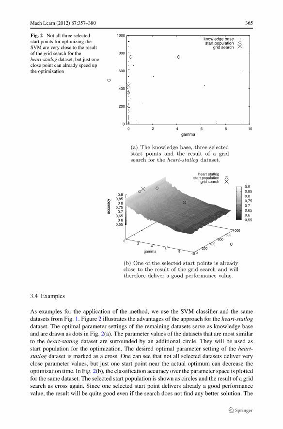
Fig. 2 Not all three selectedstart points for optimizing theSVM are very close to the resultof the grid search for theheart-statlog dataset, but just oneclose point can already speed upthe optimization

3.4 Examples

As examples for the application of the method, we use the SVM classifier and the samedatasets from Fig. 1. Figure 2 illustrates the advantages of the approach for the heart-statlogdataset. The optimal parameter settings of the remaining datasets serve as knowledge baseand are drawn as dots in Fig. 2(a). The parameter values of the datasets that are most similarto the heart-statlog dataset are surrounded by an additional circle. They will be used asstart population for the optimization. The desired optimal parameter setting of the heart-statlog dataset is marked as a cross. One can see that not all selected datasets deliver veryclose parameter values, but just one start point near the actual optimum can decrease theoptimization time. In Fig. 2(b), the classification accuracy over the parameter space is plottedfor the same dataset. The selected start population is shown as circles and the result of a gridsearch as cross again. Since one selected start point delivers already a good performancevalue, the result will be quite good even if the search does not find any better solution. The

366 Mach Learn (2012) 87:357–380

Fig. 3 If the optimization of theSVM starts with good solutions,the search will not get stuck inflat regions

second example uses the dermatology dataset and is shown in Fig. 3. Again, not the actualclosest start points were selected as shown in Fig. 3(a), but in Fig. 3(b) it is visible that allthree points have good performance values, close to the grid search result. The search willnot get stuck within the flat, black region of poor solutions.

4 Evaluation

For the evaluation of the presented approach, we used 102 classification datasets from theUCI machine learning repository (Asuncion and Newman 2007) and from StatLib (Vlachos1998), but artificially created datasets might be used as well (Frasch et al. 2011). The useddatasets from different domains contain from 10 to 2310 samples with 1 to 261 nominaland numerical attributes. A list of the datasets can be found in Table 3 in the Appendix. Sincethe training of the Random Forest classifier on the “cylinder-bands” dataset takes extremelylong, we omitted this dataset for evaluations regarding the Random Forest classifier.

Mach Learn (2012) 87:357–380 367

After the calculation of the meta-features, all datasets were preprocessed to meet therequirements of both classifiers. Missing values were replaced by the average value, nominalfeatures were converted to numerical features, and finally, all features were normalized to therange [−1;1]. The optimal parameter settings for every dataset were determined by a gridsearch and used to construct the knowledge bases for the evaluation. Regarding the SVMclassifier, the search interval for γ was [0.0001;10] with 85 logarithmic steps and [0;1000]with 100 logarithmic steps for C. Due to the computational complexity, the number of stepsfor the parameters of the Random Forest classifier were smaller. We used five steps for thenumber of trees and six steps for the remaining four parameters. This leads to 6480 classifierevaluations during the grid search, which is already a huge computational effort.

The experiments were performed by utilizing only open source libraries. LibSVM(Chang and Lin 2001) served as SVM implementation and PARF (Skala 2004) as imple-mentation for the Random Forest classifier. GAlib (Wall 1996) was used for the geneticalgorithm. We modified this genetic algorithm implementation to use a defined start popula-tion. The mutation operation was a Gaussian mutation with a step size of 1.0. Its probabilitywas selected by applying the rule of Bäck (1993): pm = 1

j, where j is the number of vari-

ables of an individual. This leads to pm = 0.5 for SVM and pm = 0.2 for Random Forest.Additionally, uniform cross-over was performed with a probability of pco = 0.9.

We compared the presented approach with five different optimization approaches:

grid search: For the SVM classifier, we applied a typical 15 × 15 grid used by Hsu andLin (2002): γ = [2−10,2−9, . . . ,24] and C = [2−2,2−1, . . . ,212]. For the Random Forestclassifier, the same grid with 6480 parameter combinations for creating the knowledgebase is used.

std. GA: The standard genetic algorithm uses a random start population. It also utilizesGAlib as implementation.

CMA: For the Covariance Matrix Adaptation Evolution Strategy (Hansen and Ostermeier2001) we used the implementation of the BEAGLE framework (Gagné and Parizeau 2006).

DIRECT: We used the NLopt (Johnson 2009) framework as implementation for the Divid-ing Rectangles algorithm (Jones et al. 1993).

GSS: Generating Set Search (Kolda et al. 2003) is a type of pattern search that can alsohandle linear constraints. HOPSPACK (Plantenga 2009) was the used implementation.

We applied all optimization methods on each of the 102 datasets using a leave-one-outcross-validation. The optimization intervals for the parameters of the SVM and RandomForest were the same as used for creating the knowledge base. Every classifier evaluationused a ten-fold cross-validation. Since the optimization runs contain random factors, 30independent runs of each algorithm were performed on every dataset. The mean accuracy ofan optimization method is the average over these 30 runs and all datasets.

All optimization methods were stopped after s generations/iterations without improve-ment. Since this parameter has a strong influence on performance and the run-time of thealgorithm, its choice is important. The influence of this parameter is discussed in more detailin Sect. 4.2.

The population-based methods contain the population size r as an additional parameter.Since the main goal of the presented approach is obtaining good solutions in a short time,small populations and rigorous stopping criteria are primarily considered. Thereby, we as-sure that the run-time of the genetic optimization is shorter than a grid search, even thoughthe standard GA typically requires a bigger population. The presented approach additionallycontains the parameter k within its meta-feature selection step (see Sect. 3.3).

An additional parameter for genetic algorithms is the used selection scheme. As alreadymentioned, a typical selection scheme is Roulette Wheel selection but rank selection may

368 Mach Learn (2012) 87:357–380

Fig. 4 Comparison of thepresented method and thestandard GA optimizing theparameters of an SVM usingdifferent selection schemes and apopulation size r = 7: bothapproaches achieve higheraccuracy values when using rankselection instead of roulettewheel selection. It is noticeablethat the improvement is biggerfor the standard GA

work better for parameter optimization. Therefore, we investigated both selection schemesfirst. Figure 4(a) shows the average accuracy of the SVM classifier achieved by the stan-dard GA and the presented approach using different stopping values and a population sizeof 7. Figure 4(b) shows a box plot of the two approaches for a stopping criterion of s = 2.It is visible that the rank-based selection scheme achieves better results for both methods.Therefore, we decided to use this selection scheme for further evaluations of the geneticalgorithms. It is also visible that the improvement by using rank selection is higher for thestandard GA.

4.1 Results and discussion

For the two datasets from the examples of Sect. 3.4, Fig. 5 shows the achieved accuracyvalues during the search for the optimal parameter values of the SVM by the standard GAand the presented approach. The values are the mean and the standard error over 30 runs.

Mach Learn (2012) 87:357–380 369

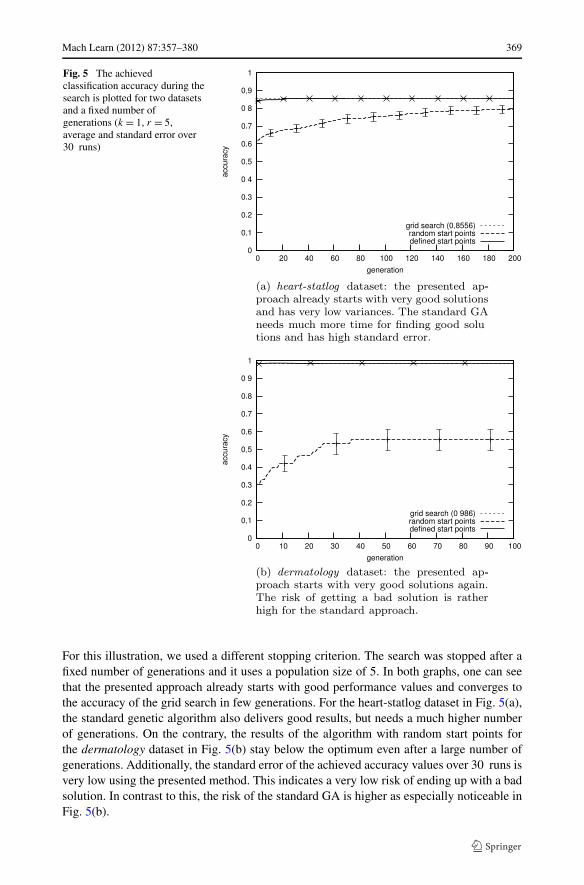
Fig. 5 The achievedclassification accuracy during thesearch is plotted for two datasetsand a fixed number ofgenerations (k = 1, r = 5,average and standard error over30 runs)

For this illustration, we used a different stopping criterion. The search was stopped after afixed number of generations and it uses a population size of 5. In both graphs, one can seethat the presented approach already starts with good performance values and converges tothe accuracy of the grid search in few generations. For the heart-statlog dataset in Fig. 5(a),the standard genetic algorithm also delivers good results, but needs a much higher numberof generations. On the contrary, the results of the algorithm with random start points forthe dermatology dataset in Fig. 5(b) stay below the optimum even after a large number ofgenerations. Additionally, the standard error of the achieved accuracy values over 30 runs isvery low using the presented method. This indicates a very low risk of ending up with a badsolution. In contrast to this, the risk of the standard GA is higher as especially noticeable inFig. 5(b).

370 Mach Learn (2012) 87:357–380

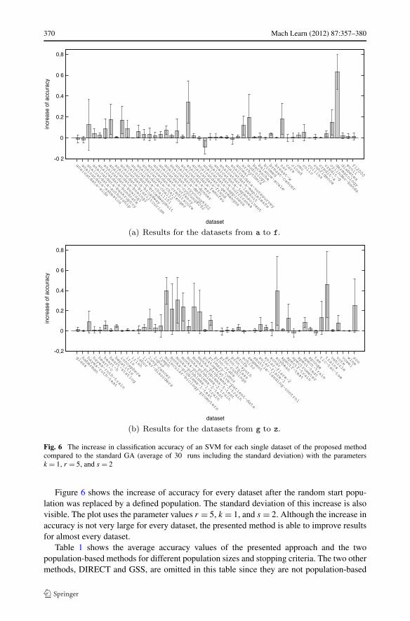
Fig. 6 The increase in classification accuracy of an SVM for each single dataset of the proposed methodcompared to the standard GA (average of 30 runs including the standard deviation) with the parametersk = 1, r = 5, and s = 2

Figure 6 shows the increase of accuracy for every dataset after the random start popu-lation was replaced by a defined population. The standard deviation of this increase is alsovisible. The plot uses the parameter values r = 5, k = 1, and s = 2. Although the increase inaccuracy is not very large for every dataset, the presented method is able to improve resultsfor almost every dataset.

Table 1 shows the average accuracy values of the presented approach and the twopopulation-based methods for different population sizes and stopping criteria. The two othermethods, DIRECT and GSS, are omitted in this table since they are not population-based

Mach Learn (2012) 87:357–380 371

Table 1 Average classification accuracy of the grid search, the standard genetic algorithm, the CMA algo-rithm and the proposed method for different parameter combinations. All values are in [%]Parameter SVM accuracy Random forest accuracy

r s Gridsearch

Std.GA

CMA Thispaper

Gridsearch

Std.GA

CMA Thispaper

3 2 81.1 70.4 69.0 79.5 80.7 68.4 68.2 77.8

5 2 81.1 72.9 69.3 80.3 80.7 71.8 68.7 78.7

5 6 81.1 74.2 70.4 80.9 80.7 73.0 69.7 79.2

7 2 81.1 74.4 69.9 81.0 80.7 73.7 69.0 79.2

7 6 81.1 75.5 70.8 81.2 80.7 74.7 69.7 79.7

7 10 81.1 76.4 71.0 81.8 80.7 74.9 70.1 80.0

and a comparison considering population sizes is not easily possible. The accuracy achievedby the grid search is also shown. It is visible that the presented method achieves higher ac-curacy values than the standard GA and CMA for both classification algorithms. For r = 7and s = 10, the presented method achieves an even higher accuracy than grid search for theSVM classifier.

To decide whether these differences in accuracy are statistically significant or not, weapplied statistical tests over the 102 datasets and compared the presented approach witheach competing method. To do this, the paired t -test might be used. However, this paramet-ric test assumes that the accuracy differences are normally distributed. Furthermore, outliersin the tested population decreases the power of the t -test (Demšar 2006). Since the resultsparticularly contain outliers, we used the non-parametric Wilcoxon test instead. For all con-sidered parameter combinations and a confidence level of 95 %, the differences betweenthe proposed method and the grid search are not statistically significant whereas the dif-ferences between the proposed method and the std. GA as well as the CMA are indeedsignificant.

In addition to the accuracy, we compared the run-time of the different approaches. Fig-ure 7 shows the accuracy depending on the number of evaluations for two different pop-ulation sizes. The presented approach achieves higher accuracies for both classifiers for adifferent number of classifier evaluations. The standard GA and the CMA method are unableto achieve the same accuracy even for higher number of evaluations. Surprisingly, the CMAalgorithm is worse than the standard GA for approximately the same number of evaluations.

Summarizing, the presented method is able to reach performance values of a grid search,but only needs the time of a genetic algorithm. For example, using an AMD Opteron with2.3 GHz, the presented approach needs only about 45 minutes for optimizing the SVMparameters of all datasets using the parameter values r = 7 and s = 2. The grid search needsabout six hours that is consequently more than seven times longer. However, the differenceof the achieved average accuracy values of 81.0 % by the presented method and 81.1 % bythe grid search is statistically not significant.

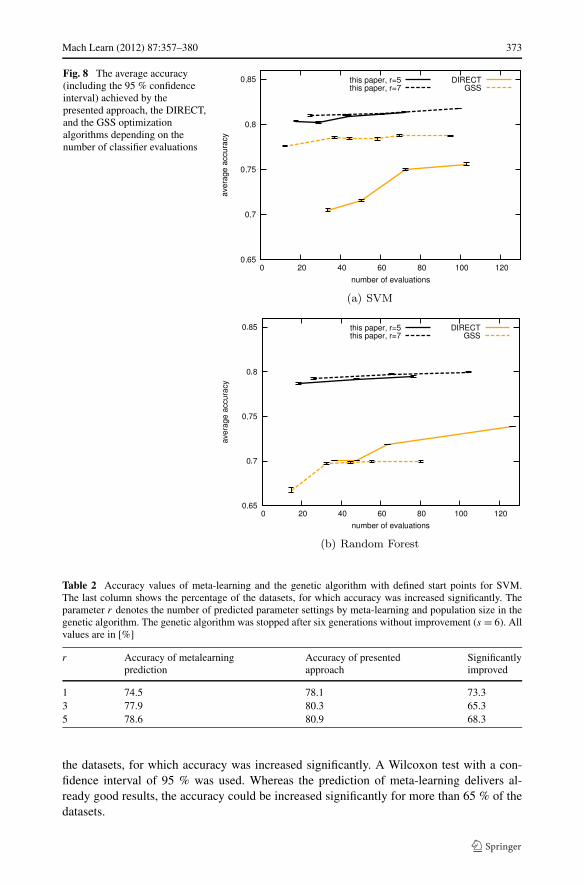
Since the two optimization methods DIRECT and GSS do not use any population, theclassifier is evaluated only once during an iteration of the search. Therefore, a large numberof iterations without improvement were allowed to assure a fairer comparison. However, asvisible in Fig. 8, both methods do not reach the accuracy values of the presented approachfor a comparable number of classifier evaluations. Although the GSS algorithm deliversgood results for the SVM classifier, the achieved accuracy values are lower than the std. GAfor the Random Forest classifier.

372 Mach Learn (2012) 87:357–380

Fig. 7 The average accuracy(including the 95 % confidenceinterval) achieved by thepresented approach and thecompeting population-basedmethods depending on thenumber of classifier evaluations

For the Wilcoxon tests of the accuracy differences over the datasets, we used those of theconsidered parameter combinations of the algorithms on which they achieved their highestaverage accuracy. With a confidence level of 95 %, the differences between the presentedmethod and GSS as well as DIRECT are statistically significant. Only the difference forSVM with GSS is statistically not significant.

Furthermore, we investigated how much accuracy could be achieved purely by meta-learning without any evolutionary optimization. For that purpose, we evaluated the perfor-mance of the parameter predictions directly. Predicted parameter settings are the optimalparameter values of the r most similar datasets. The performance of the predictions is thehighest accuracy achieved with one of those unmodified settings. Table 2 shows the per-formance of the predictions for the SVM classifier. Besides, the predicted parameter valueswere used as start points for the genetic algorithm to quantify the improvement in accuracydue to the optimization step. The results show that the following evolutionary optimiza-tion is able to improve the performance values. The last column shows the percentage of

Mach Learn (2012) 87:357–380 373

Fig. 8 The average accuracy(including the 95 % confidenceinterval) achieved by thepresented approach, the DIRECT,and the GSS optimizationalgorithms depending on thenumber of classifier evaluations

Table 2 Accuracy values of meta-learning and the genetic algorithm with defined start points for SVM.The last column shows the percentage of the datasets, for which accuracy was increased significantly. Theparameter r denotes the number of predicted parameter settings by meta-learning and population size in thegenetic algorithm. The genetic algorithm was stopped after six generations without improvement (s = 6). Allvalues are in [%]

r Accuracy of metalearningprediction

Accuracy of presentedapproach

Significantlyimproved

1 74.5 78.1 73.33 77.9 80.3 65.35 78.6 80.9 68.3

the datasets, for which accuracy was increased significantly. A Wilcoxon test with a con-fidence interval of 95 % was used. Whereas the prediction of meta-learning delivers al-ready good results, the accuracy could be increased significantly for more than 65 % of thedatasets.

374 Mach Learn (2012) 87:357–380

Fig. 9 The influence of thepopulations size r for threedifferent values of s. Smallerpopulations sizes already reachgood performance values

4.2 Effect of changes in parameter values

Previously, only exemplary values of the parameters k, r , and s have been investigated,although the choice of the parameters can have a strong influence on the results of anoptimization method. Bartz-Beielstein et al. (2005) presented an approach for optimizingthe parameters of search heuristics which can also be used to optimize different parame-ters of genetic algorithms. However, instead of such an additional optimization, we did anextensive manual analysis of the parameters of the presented method for the SVM classi-fier.

The parameter k is the number of neighbors, whose distance is minimized during themeta-feature selection step. Since only one good prediction is sufficient for improving thegenetic algorithm, a value of one seems to be a good choice, independently from the otherparameters. Therefore, we omitted the genetic algorithm and computed only the accuracyvalues achieved by the potential start points. Our experiments showed that for small values

Mach Learn (2012) 87:357–380 375

Fig. 10 The influence of theparameter s of the stoppingcriterion for two differentpopulation sizes. Rigorousstopping criteria (small valuesof s) only slightly reduce theaverage accuracy of the presentedapproach

of k, the results differ not much and k = 1 seems to be a good choice in general. So we stickto this value for the evaluation of the two other parameters.

The population size r is an important parameter of genetic algorithms. Smaller popu-lation sizes reduce the computation time, but may miss good results as well. The averageaccuracy values achieved by the SVM with different population sizes are plotted in Fig. 9(a)for both approaches. Although very small population sizes are uncommon for genetic al-gorithms, the presented approach already reaches good performance results using these set-tings. The performance of the standard approach stays below the presented method for eachconsidered population size.

Figure 9(b) shows the average number of generations for both methods. It is visible thatan increase in the population size does not lead to fewer generations in general. However,the average number of generations for the presented method were lower than those for thestandard genetic algorithm.

For the parameter s of the stopping criterion, Fig. 10 shows the average accuracy andnumber of generations. A more rigorous stopping did not lead to much worse results of the

376 Mach Learn (2012) 87:357–380

presented method (Fig. 10(a)), but can shorten the search time dramatically (Fig. 10(b)).Again, parameter values that will lead to a shorter run-time (like small values of s) increasethe benefit of the presented approach.

5 Conclusion

In this paper, a new approach of using meta-learning in genetic algorithms for parameteroptimization of classifiers was presented. Knowledge based on previous evaluations on sim-ilar datasets was used to define a better initial population instead of random individuals. Thesimilarity between datasets was computed as a function of distance between their automati-cally selected meta-features.

Our approach was used for optimizing two parameters of Support Vector Machines(SVM) and five parameters of the Random Forest classifier on over 100 datasets from theUCI and StatLib repositories. The results showed that the presented approach is able tosignificantly increase the average classification accuracy of both classifiers compared to astandard genetic algorithm. The achieved accuracy values of the SVM were close to thoseachieved by a typical 15×15 grid search for SVMs at one-seventh of the computational cost.Moreover, the presented approach was compared to three other state-of-the-art optimizationalgorithms. The results show that it achieves the best average accuracy for both classifiers.

Acknowledgements This work was partially funded by the BMBF (German Federal Ministry of Educationand Research), project PaREn (01 IW 07001). We also thank the reviewers for their detailed and helpfulcomments to the manuscript.

Appendix: Increase of accuracy

Table 3 The increase of accuracy of the presented method compared to the standard GA for each datasetand different parameter combinations (averaged over 30 runs)

Dataset SVM Random forest

r = 5 r = 7 r = 5 r = 7

s = 2 s = 6 s = 2 s = 6 s = 2 s = 6 s = 2 s = 6

Analcatdata-aids −1.8 −1.0 −0.6 −1.0 8.5 8.0 7.0 9.1

Analcatdata-asbestos −2.9 −1.8 −2.4 −2.2 1.9 2.8 3.3 2.4

Analcatdata-authorship 10.4 12.5 10.4 4.2 0.9 0.8 0.8 0.9

Analcatdata-bankruptcy 3.9 4.1 4.5 4.3 21.1 20.5 15.9 8.9

Analcatdata-bondrate 2.1 2.4 2.4 1.6 1.0 0.8 0.9 1.0

Analcatdata-boxing1 10.3 8.7 9.6 8.3 9.5 9.2 7.6 5.8

Analcatdata-boxing2 17.5 17.7 11.9 10.3 12.0 6.9 11.2 2.8

Analcatdata-braziltourism 0.7 0.9 1.0 0.8 0.2 −0.1 0.0 0.3

Analcatdata-broadway 12.6 17.0 11.5 9.1 8.1 4.5 8.4 4.7

Analcatdata-broadwaymult 10.1 8.6 9.0 6.6 −1.4 −1.0 −1.4 −0.1

Analcatdata-chall101 0.0 0.0 0.0 0.0 0.0 0.0 0.0 0.0

Analcatdata-chall2 6.2 6.2 7.1 3.0 4.4 1.3 4.1 3.7

Analcatdata-challenger 5.1 3.0 1.7 0.4 7.8 7.0 6.8 7.2

Analcatdata-creditscore 3.7 3.5 0.2 0.1 4.9 6.1 1.6 1.8

Mach Learn (2012) 87:357–380 377

Table 3 (Continued)

Dataset SVM Random forest

r = 5 r = 7 r = 5 r = 7

s = 2 s = 6 s = 2 s = 6 s = 2 s = 6 s = 2 s = 6

Analcatdata-currency −0.2 1.7 −0.6 −0.5 1.9 1.7 1.7 2.8Analcatdata-cyyoung8092 4.7 3.3 4.9 5.4 2.8 3.4 4.0 3.3Analcatdata-cyyoung9302 6.3 7.2 6.8 5.8 4.0 3.5 3.0 3.0Analcatdata-dmft 2.4 2.2 2.0 2.4 1.0 0.2 0.3 0.1Analcatdata-donner 6.7 6.8 17.0 13.0 12.2 10.3 9.1 10.0Analcatdata-esr 0.9 1.1 0.9 1.7 1.0 1.1 1.9 2.6Analcatdata-famufsu 36.4 34.3 41.4 33.1 47.2 47.3 38.7 41.5Analcatdata-fraud 2.2 2.1 3.3 2.5 4.9 3.8 5.1 3.5Analcatdata-germangss 0.0 −0.5 −0.8 0.2 2.0 1.2 1.5 0.8Analcatdata-happiness −10.1 −9.1 −1.4 −1.4 12.8 13.9 13.4 12.2Analcatdata-hurricanes 1.2 0.8 0.8 0.8 −1.3 −1.8 0.2 0.2Analcatdata-japansolvent 0.3 0.8 1.7 1.2 17.3 14.9 7.1 10.7Analcatdata-lawsuit 0.8 0.7 1.1 0.8 0.8 1.1 0.8 1.2Analcatdata-mapleleafs 0.3 0.9 0.3 0.4 0.1 0.1 −0.1 0.0Analcatdata-votesurvey −4.6 −1.4 −3.8 −3.1 8.6 10.0 10.3 4.1Anneal 0.8 1.4 1.3 1.3 2.1 2.3 6.1 4.0Arrhythmia 14.0 11.8 10.3 9.3 4.4 3.1 3.5 2.0Audiology 19.6 19.7 28.2 24.3 19.7 17.4 15.9 15.6Backache 0.5 0.7 0.6 0.9 0.5 0.7 0.4 0.9Balance-scale 3.4 1.4 2.5 2.1 2.6 1.5 1.6 0.8Biomed −0.1 −0.1 −0.3 −0.2 2.2 1.6 1.9 1.4Breast-cancer 4.4 3.7 4.1 3.6 −1.1 −1.3 −0.3 −1.5Breast-w 0.4 0.3 0.4 0.3 0.4 0.2 0.3 0.3Car 15.7 18.0 10.9 7.1 9.6 6.8 6.0 4.5Cars 0.4 0.2 1.6 2.3 6.5 8.1 6.6 5.8Cloud −0.1 0.4 −0.4 0.3 9.7 9.5 8.0 6.6Cmc 2.8 2.4 2.3 1.4 0.1 −1.0 −0.7 −0.2Colic 9.1 5.2 4.7 5.3 0.7 0.3 0.4 0.3Collins 0.0 0.0 0.2 0.0 5.6 4.6 4.1 4.3Confidence 0.7 0.9 0.8 1.1 38.9 37.9 23.1 25.7Credit-a 1.3 0.3 0.4 0.5 0.5 0.7 0.4 0.3Credit-g 4.7 4.0 4.2 3.9 2.0 1.2 1.1 1.1Cylinder-bands 14.5 15.1 12.6 11.1 – – – –Dermatology 49.7 63.2 49.7 56.5 6.1 3.7 2.9 2.0Diabetes 3.0 1.9 1.7 1.4 0.6 0.1 0.2 −0.1Ecoli 2.2 1.4 1.7 1.2 1.8 2.2 4.4 3.0Fl2000 1.9 1.3 1.3 1.3 7.3 10.0 5.9 5.5Glass 1.7 1.5 0.5 0.9 7.5 8.5 6.9 7.2Haberman −0.2 0.2 0.1 −0.1 0.2 0.4 0.2 0.1Hayes-roth-test 8.1 8.8 6.0 7.3 23.8 15.4 15.1 19.2Hayes-roth-train 1.2 1.0 1.2 1.2 7.7 5.1 6.0 7.3Heart-c 3.1 1.0 2.2 0.2 0.4 −0.1 0.2 0.2Heart-h 8.1 6.0 7.1 6.1 0.0 0.2 0.0 0.6Heart-statlog 2.3 0.5 0.6 0.2 0.5 0.8 0.5 0.3

378 Mach Learn (2012) 87:357–380

Table 3 (Continued)

Dataset SVM Random forest

r = 5 r = 7 r = 5 r = 7

s = 2 s = 6 s = 2 s = 6 s = 2 s = 6 s = 2 s = 6

Hepatitis 5.0 4.9 4.9 4.8 1.9 1.1 2.5 2.3Ionosphere 1.2 0.2 0.7 0.2 3.3 1.4 1.6 1.3Iris 1.4 1.2 1.3 1.4 5.8 5.8 5.0 0.1Irish 0.4 0.3 0.3 0.2 1.9 0.1 0.4 0.0Labor 8.4 1.2 7.4 1.7 7.9 9.9 13.7 5.3Liver-disorders 3.6 3.5 2.7 2.6 0.7 0.6 1.7 1.1Lung-cancer 13.5 11.9 11.9 14.6 12.8 13.3 13.6 11.9Lupus 3.4 2.5 1.8 1.3 1.1 3.2 1.1 0.5Lymph 12.7 4.8 9.1 2.7 4.1 3.5 4.4 4.8Molecular-biology-promoters 35.8 39.9 32.9 27.5 4.5 6.4 2.3 2.5Monks-problems-1-test 30.0 21.7 13.3 18.3 23.0 14.3 13.8 10.2Monks-problems-1-train 37.7 30.4 30.6 23.3 20.1 16.9 14.9 16.8Monks-problems-2-test 31.8 24.0 26.2 22.2 20.2 17.9 20.3 18.0Monks-problems-2-train 5.7 4.5 9.7 10.6 3.8 4.6 4.4 5.7Monks-problems-3-test 18.2 23.6 12.6 17.3 8.5 2.3 4.6 2.1Monks-problems-3-train 30.5 18.9 24.6 17.3 11.4 4.9 5.0 2.3Postoperative-patient-data 0.4 0.6 0.8 0.9 0.2 0.0 0.1 0.3Primary-tumor 9.0 10.5 9.9 7.4 3.4 2.8 3.1 4.1Prnn-crabs 0.4 0.1 0.2 0.1 14.2 8.8 8.2 7.2Prnn-cushings −0.1 −0.5 0.6 1.2 20.4 21.1 21.1 16.6Prnn-fglass 1.4 1.1 0.8 0.5 10.6 8.7 11.7 8.5Prnn-synth 0.3 0.6 0.2 0.1 1.0 −0.4 −0.2 −0.3Profb 4.5 3.9 4.7 4.4 −0.8 −0.3 −0.4 −0.1Schizo −0.3 −0.7 −0.1 −0.2 4.6 4.3 1.6 4.3Segment 0.0 −0.1 0.0 −0.1 1.5 1.0 1.1 1.0Shuttle-landing-control 0.2 0.4 0.0 0.2 −0.5 2.0 1.0 −2.2Solar-flare-1 10.3 6.4 8.8 8.6 2.5 0.8 0.8 0.0Solar-flare-2 3.6 3.6 2.7 2.7 0.5 0.4 0.3 0.2Sonar 4.2 1.6 0.8 1.9 5.2 6.7 3.7 3.2Soybean 48.7 39.5 44.0 37.3 10.9 7.4 4.5 8.0Spectf-test 1.3 1.2 1.4 1.0 −0.3 0.0 −0.4 0.2Spectf-train 11.8 12.5 9.0 8.0 9.7 11.7 8.5 6.8Spectrometer 0.7 −2.3 3.9 1.7 10.6 11.6 7.8 9.1Spect-test 0.3 0.2 0.1 0.2 0.1 0.2 0.3 0.2Spect-train 9.4 8.4 8.0 6.8 11.4 8.8 4.3 4.9Sponge 2.2 2.1 2.1 1.5 2.3 1.8 1.6 1.2Tae −2.8 −1.6 −1.3 −2.6 14.0 13.4 10.9 12.8Tic-tac-toe 26.8 13.1 15.5 14.2 12.5 10.6 7.8 7.8Trains 40.7 46.0 43.3 29.3 33.0 42.3 40.7 33.3Vehicle 1.5 0.5 0.9 0.2 3.8 2.8 3.8 2.2Vote 9.5 8.0 8.0 6.9 2.1 1.1 1.0 1.0Vowel 0.2 0.1 0.0 0.1 17.7 19.4 11.8 9.4Wine 0.2 0.0 0.1 0.1 3.8 3.3 3.1 3.5Zoo 35.0 25.0 21.3 26.0 14.4 8.8 13.3 14.1

Mach Learn (2012) 87:357–380 379

References

Ali, S., & Smith, K. A. (2006). On learning algorithm selection for classification. Applied Soft Computing, 6,119–138.

Asuncion, A., & Newman, D. (2007). UCI machine learning repository. University of California, Irvine,School of Information and Computer Sciences. http://www.ics.uci.edu/~mlearn/MLRepository.html.

Ayat, N., Cheriet, M., & Suen, CY (2002). Optimization of the SVM kernels using an empirical error min-imization scheme. In Proc. of the international workshop on pattern recognition with support vectormachine (pp. 354–369). Berlin: Springer.

Bäck, T. (1993). Optimal mutation rates in genetic search. In Proceedings of the fifth international conferenceon genetic algorithms (pp. 2–8). San Francisco: Morgan Kaufmann.

Bartz-Beielstein, T., Lasarczyk, C. W. G., & Preuss, M. (2005). Sequential parameter optimization. 2005IEEE congress on evolutionary computation (Vol. 1, pp. 773–780). New York: IEEE Press

Bensusan, H., & Giraud-Carrier, C. (2000a). Casa batló is in passeig de gràcia or how landmark performancescan describe tasks. In Proceedings of the ECML-00 workshop on meta-learning: Building automaticadvice strategies for model selection and method combination (pp. 29–46).

Bensusan, H., & Giraud-Carrier, C. G. (2000b). Discovering task neighbourhoods through landmark learningperformances. In PKDD’00: Proceedings of the 4th European conference on principles of data miningand knowledge discovery (pp. 325–330). London: Springer.

Bensusan, H., & Kalousis, A. (2001) Estimating the predictive accuracy of a classifier. In L. De Raedt,& P. Flach (Eds.), Lecture notes in computer science: Vol. 2167. Machine learning: ECML 2001(pp. 25–36). Berlin: Springer.

Berrer, H., Paterson, I., & Keller, J. (2000). Evaluation of machine-learning algorithm ranking advisors. InProceedings of the PKDD-2000 workshop on datamining, decision support, meta-learning and ILP:Forum for practical problem presentation and prospective solutions.

Brazdil, P., Gama, J., & Henery, B (1994). Characterizing the applicability of classification algorithms us-ing meta-level learning. In: ECML-94: Proceedings of the European conference on machine learning(pp. 83–102). Secaucus: Springer.

Brazdil, P., Soares, C., & da Costa, J. P. (2003). Ranking learning algorithms: Using ibl and meta-learning onaccuracy and time results. Machine Learning, 50(3), 251–277.

Breiman, L. (2001). Random forests. Machine Learning, 45, 5–32.Burges, C. J. (1998). A tutorial on support vector machines for pattern recognition. Data Mining and Knowl-

edge Discovery, 2, 121–167.Chang, C. C., & Lin, C. J. (2001). LIBSVM: a library for support vector machines. Software available at

http://www.csie.ntu.edu.tw/~cjlin/libsvm.Chapelle, O., Vapnik, V., Bousquet, O., & Mukherjee, S. (2002). Choosing multiple parameters for support

vector machines. Machine Learning, 46, 131–159.Cortes, C., & Vapnik, V. (1995). Support-vector networks. Machine Learning, 20(3), 273–297.Demšar, J. (2006). Statistical comparisons of classifiers over multiple data sets. Journal of Machine Learning

Research, 7, 1–30.Eitrich, T., & Lang, B. (2006). Efficient optimization of support vector machine learning parameters for

unbalanced datasets. Journal of Computational and Applied Mathematics, 196(2), 425–436.Engels, R., & Theusinger, C. (1998). Using a data metric for preprocessing advice for data mining applica-

tions. In: Proceedings of the European conference on artificial intelligence (pp. 430–434). New York:Wiley.

Frasch, J. V., Lodwich, A., Shafait, F., & Breuel, T. M. (2011). A bayes-true data generator for evaluation ofsupervised and unsupervised learning methods. Pattern Recognition Letters, 32(11), 1523–1531.

Friedrichs, F., & Igel, C. (2005). Evolutionary tuning of multiple SVM parameters. Neurocomputing, 64,107–117.

Gagné, C., & Parizeau, M. (2006). Genericity in evolutionary computation software tools: Principles and casestudy. International Journal on Artificial Intelligence Tools, 15(2), 173–194.

Gama, J., & Brazdil, P. (1995). Characterization of classification algorithms. In C. Pinto-Ferreira &N. Mamede (Eds.), Lecture notes in computer science: Vol. 990. Progress in artificial intelligence(pp. 189–200). Berlin: Springer.

Goldberg, D. E. (1989). Genetic algorithms in search, optimization, and machine learning (1st ed.) Reading:Addison-Wesley.

Hansen, N., & Ostermeier, A. (2001). Completely derandomized self-adaptation in evolution strategies. Evo-lutionary Computation, 9(2), 159–195.

Hilario, M., Nguyen, P., Do, H., Woznica, A., & Kalousis, A. (2011). Ontology-based meta-mining of knowl-edge discovery workflows. In N. Jankowski, W. Duch, & K. Grabczewski (Eds.), Meta-learning in com-putational intelligence, studies in computational intelligence (Vol. 358, pp. 273–315). Berlin: Springer.

380 Mach Learn (2012) 87:357–380

Hsu, C. W., & Lin, C. J. (2002). A comparison of methods for multi-class support vector machines. IEEETransactions on Neural Networks, 13, 415–425.

Johnson, S. G. (2009). The nlopt nonlinear-optimization package. http://ab-initio.mit.edu/nlopt.Jones, D. R., Perttunen, C. D., & Stuckman, B. E. (1993). Lipschitzian optimization without the Lipschitz

constant. Journal of Optimization Theory and Applications, 79(1), 157–181.Kalousis, A., & Hilario, M. (2001). Feature selection for meta-learning. In D. Cheung, G. Williams, & Q. Li

(Eds.), Lecture notes in computer science: Vol. 2035. Advances in knowledge discovery and data mining(pp. 222–233). Berlin: Springer.

Kietz, J. U., Serban, F., Bernstein, A., & Fischer, S. (2010). Data mining workflow templates for intelligentdiscovery assistance and auto-experimentation. In Proceedings of the ECML/PKDD-10 workshop onthird generation data mining: Towards service-oriented knowledge discovery (pp. 1–12).

King, R. D., Feng, C., & Sutherland, A. (1995). Statlog: Comparison of classification algorithms on largereal-world problems. Applied Artificial Intelligence, 9(3), 289–333.

Kohonen, T. (1998). Learning vector quantization. In The handbook of brain theory and neural networks(pp. 537–540). Cambridge: MIT Press.

Kolda, T. G., Lewis, R. M., & Torczon, V. (2003). Optimization by direct search: New perspectives on someclassical and modern methods. SIAM Review, 45, 385–482.

Köpf, C., Taylor, C., & Keller, J. (2000). Meta-analysis: From data characterisation for meta-learning to meta-regression. In Proceedings of the PKDD-00 workshop on data mining, decision support, meta-learningand ILP.

Merelo, J. J., Prieto, A., & Morán, F. (2001). Optimization of classifiers using genetic algorithms. In M. Pa-tel, V. Honavar, & K. Balakrishnan (Eds.), Advances in the evolutionary synthesis of intelligent agents(pp. 91–108). Cambridge: MIT Press.

Merz, C. (1995) Dynamical selection of learning algorithms. In Learning from data, artificial intelligenceand statistics. Berlin: Springer.

Momma, M., & Bennett, K. P. (2002). A pattern search method for model selection of support vector regres-sion. In Proceedings of the SIAM international conference on data mining.

Pfahringer, B., Bensusan, H., & Giraud-Carrier, C. (2000). Meta-learning by landmarking various learningalgorithms. In Proceedings of the seventeenth international conference on machine learning (pp. 743–750). San Mateo: Morgan Kaufmann.

Plantenga, T. D. (2009). Hopspack 2.0 user manual (Tech. Rep. SAND2009-6265). Sandia National Labora-tories, Albuquerque, NM and Livermore, CA.

Shafait, F., & Breuel, T. M. (2011). The effect of border noise on the performance of projection-based pagesegmentation methods. IEEE Transactions on Pattern Analysis and Machine Intelligence, 33(4), 846–851.

Skala, K. (2004). PARF—Parallel RF algorithm. Centre for Informatics and Computing of Ruder BoškovicInstitute. http://www.irb.hr/en/research/projects/it/2004/2004-111/.

Smith-Miles, K. A. (2008). Cross-disciplinary perspectives on meta-learning for algorithm selection. ACMComputing Surveys, 41(1), 1–25.

Soares, C., & Brazdil, P. B. (2006). Selecting parameters of SVM using meta-learning and kernel matrix-based meta-features. In SAC’06: Proceedings of the 2006 ACM symposium on applied computing(pp. 564–568). New York: ACM.

Soares, C., Brazdil, P. B., & Kuba, P. (2004). A meta-learning method to select the kernel width in supportvector regression. Machine Learning, 54(3), 195–209.

Sohn, S. Y. (1999). Meta analysis of classification algorithms for pattern recognition. IEEE Transactions onPattern Analysis and Machine Intelligence, 21(11), 1137–1144.

Vilalta, R., Giraud-carrier, C., Brazdil, P., & Soares, C. (2004). Using meta-learning to support data mining.International Journal of Computer Science and Applications, 1(1), 31–45.

Vlachos, P. (1998). StatLib datasets archive. Department of Statistics, Carnegie Mellon University. http://lib.stat.cmu.edu/l.

Wall, M. (1996). Galib: A C++ library of genetic algorithm components. Mechanical Engineering Depart-ment, Massachusetts Institute of Technology.

Yao, X. (1993). Evolutionary artificial neural networks. International Journal of Intelligent Systems, 4, 539–567.