Meta-analysis of diagnostic test accuracy studies … of diagnostic test accuracy studies with...

Meta-analysis of diagnostic test accuracy studies with Stata: Simulation study

}  Nieves Plana, Víctor Abraira, Javier Zamora

}  Unidad de Bioestadística Clínica. Hospital Ramón y Cajal, IRYCIS. Madrid

}  CIBER Epidemiología y Salud Pública (CIBERESP)

1

Contents

10 de Octubre de 2013 2

} Background

} Aims

} Methods

} Results

} Conclusions & Further works

TP

FN

FP

TN

+

-

Si No SoT

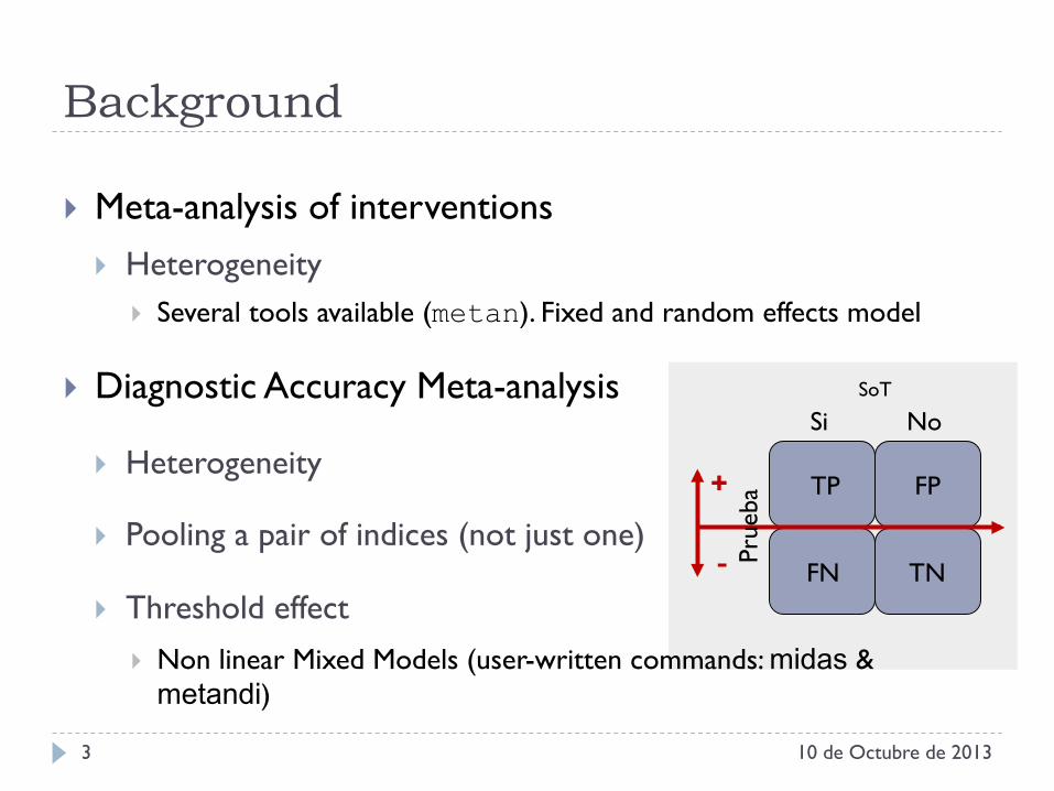
Background

10 de Octubre de 2013

}  Meta-analysis of interventions }  Heterogeneity

}  Several tools available (metan). Fixed and random effects model

}  Diagnostic Accuracy Meta-analysis

}  Heterogeneity

}  Pooling a pair of indices (not just one)

}  Threshold effect }  Non linear Mixed Models (user-written commands: midas &

metandi)

3 Pr

ueba

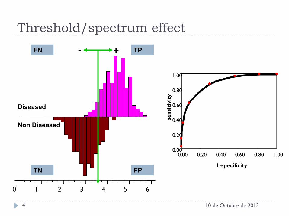
Threshold/spectrum effect


Diseased

0 1 2 3 4 5 6

Non Diseased

TP

FP

FN

TN

+ -

1-specificity

0.00

0.20

0.40

0.60

0.80

1.00

0.00 0.20 0.40 0.60 0.80 1.00 se

nsit

ivit

y

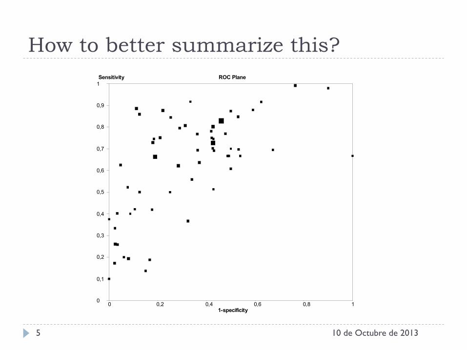
How to better summarize this?


Sensitivity ROC Plane

1-specificity0 0,2 0,4 0,6 0,8 1

0

0,1

0,2

0,3

0,4

0,5

0,6

0,7

0,8

0,9

1

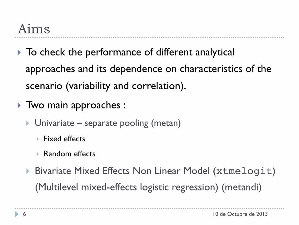
Aims

}  To check the performance of different analytical

approaches and its dependence on characteristics of the

scenario (variability and correlation).

}  Two main approaches :

}  Univariate – separate pooling (metan)

}  Fixed effects

}  Random effects

}  Bivariate Mixed Effects Non Linear Model (xtmelogit)

(Multilevel mixed-effects logistic regression) (metandi)


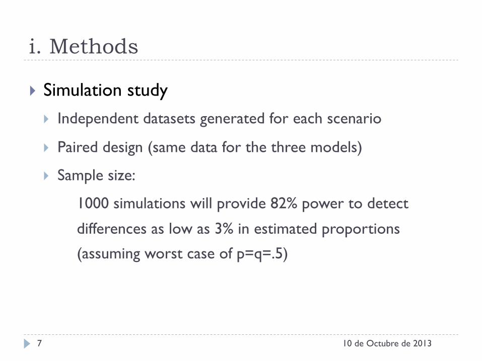
i. Methods

}  Simulation study }  Independent datasets generated for each scenario

}  Paired design (same data for the three models)

}  Sample size:

1000 simulations will provide 82% power to detect

differences as low as 3% in estimated proportions

(assuming worst case of p=q=.5)


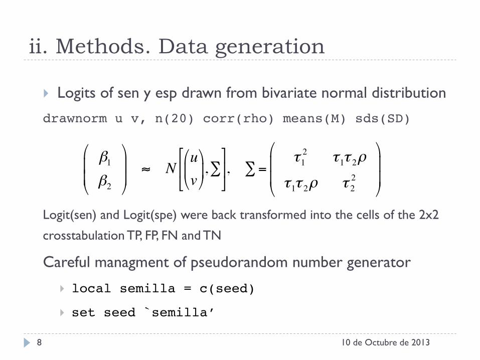
ii. Methods. Data generation

}  Logits of sen y esp drawn from bivariate normal distribution

drawnorm u v, n(20) corr(rho) means(M) sds(SD)!

!

!

!

Logit(sen) and Logit(spe) were back transformed into the cells of the 2x2

crosstabulation TP, FP, FN and TN

Careful managment of pseudorandom number generator

}  local semilla = c(seed)!

}  set seed `semilla’!


β1β2

!

"

##

$

%

&& ≈ N

uv!

"#$

%&,∑

)

*+

,

-., ∑ =

τ12 τ1τ 2ρ

τ1τ 2ρ τ 22

!

"

##

$

%

&&

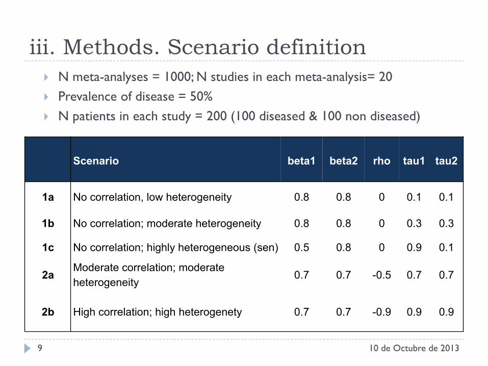
iii. Methods. Scenario definition }  N meta-analyses = 1000; N studies in each meta-analysis= 20 }  Prevalence of disease = 50% }  N patients in each study = 200 (100 diseased & 100 non diseased)


Scenario beta1 beta2 rho tau1 tau2

1a No correlation, low heterogeneity 0.8 0.8 0 0.1 0.1

1b No correlation; moderate heterogeneity 0.8 0.8 0 0.3 0.3

1c No correlation; highly heterogeneous (sen) 0.5 0.8 0 0.9 0.1

2a Moderate correlation; moderate heterogeneity

0.7 0.7 -0.5 0.7 0.7

2b High correlation; high heterogenety 0.7 0.7 -0.9 0.9 0.9

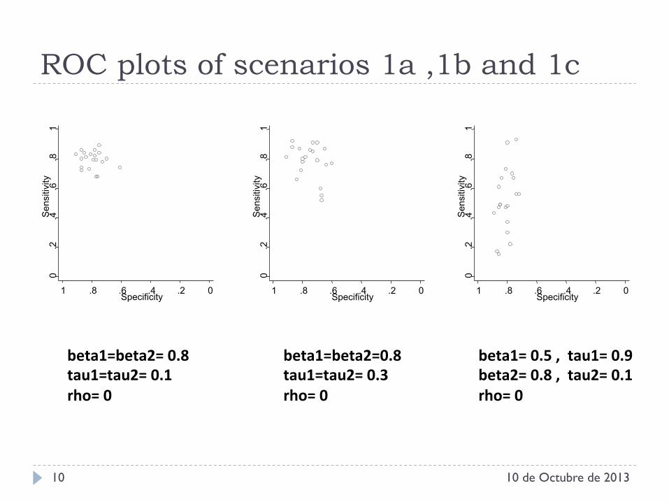
ROC plots of scenarios 1a ,1b and 1c


beta1=beta2= 0.8 tau1=tau2= 0.1 rho= 0

beta1=beta2=0.8 tau1=tau2= 0.3 rho= 0

0 .2

.4

.6

.8

1 S

ensi

tivity

0 .2 .4 .6 .8 1 Specificity

0 .2

.4

.6

.8

1 S

ensi

tivity


0 .2

.4

.6

.8

1 S

ensi

tivity


beta1= 0.5 , tau1= 0.9 beta2= 0.8 , tau2= 0.1 rho= 0

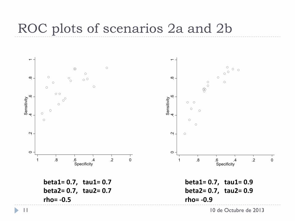
ROC plots of scenarios 2a and 2b


beta1= 0.7, tau1= 0.9 beta2= 0.7, tau2= 0.9 rho= -‐0.9

beta1= 0.7, tau1= 0.7 beta2= 0.7, tau2= 0.7 rho= -‐0.5

0 .2

.4

.6

.8

1 S

ensi

tivity


0 .2

.4

.6

.8

1 S

ensi

tivity


iv. Methods

}  Statistics for comparison (user written command

simsum):

}  BIAS

}  PRECISION: empirical standard error and RMS model-based

standard error

}  COVERAGE of 95% CI

}  Software : Stata version12


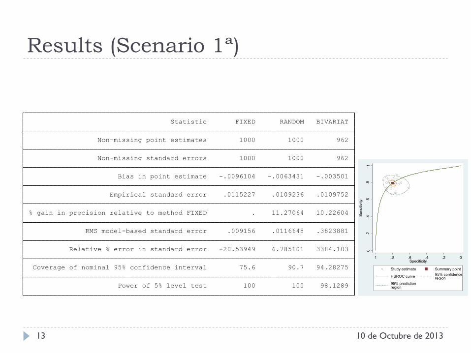
Results (Scenario 1ª)


0.2

.4.6

.81

Sen

sitiv

ity

0.2.4.6.81Specificity

Study estimate Summary point

HSROC curve 95% confidenceregion

95% predictionregion

Power of 5% level test 100 100 98.1289 Coverage of nominal 95% confidence interval 75.6 90.7 94.28275 Relative % error in standard error -20.53949 6.785101 3384.103 RMS model-based standard error .009156 .0116648 .3823881 % gain in precision relative to method FIXED . 11.27064 10.22604 Empirical standard error .0115227 .0109236 .0109752 Bias in point estimate -.0096104 -.0063431 -.003501 Non-missing standard errors 1000 1000 962 Non-missing point estimates 1000 1000 962 Statistic FIXED RANDOM BIVARIAT

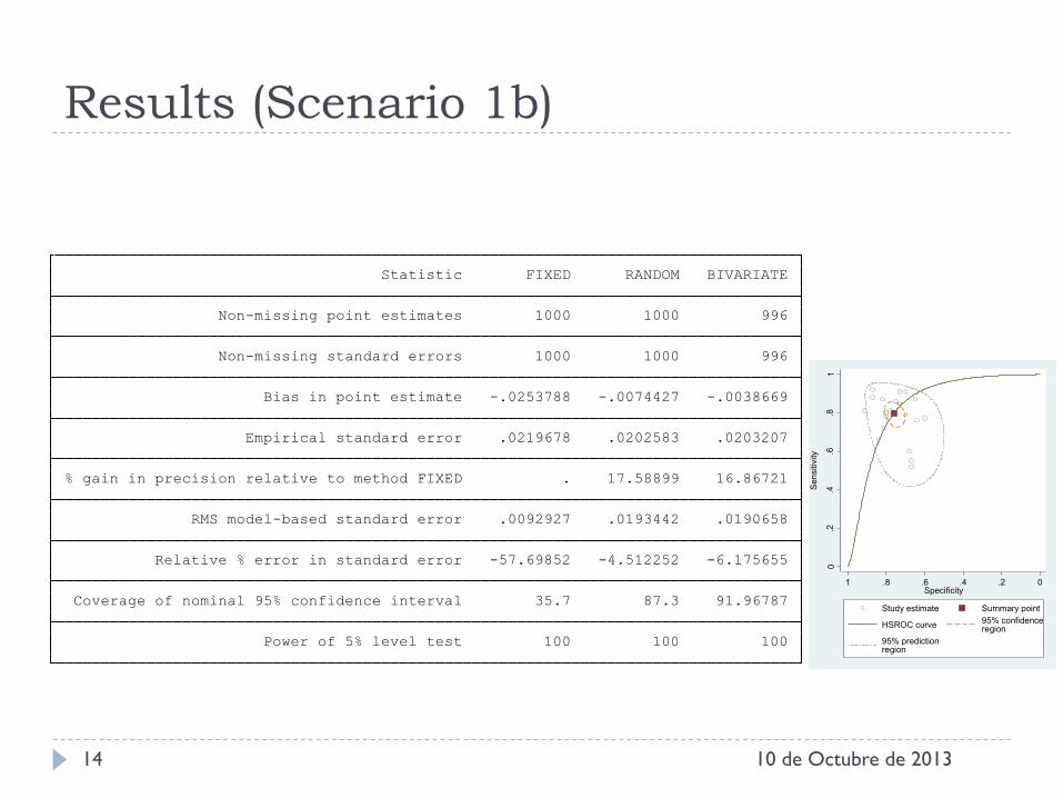
Results (Scenario 1b)


Power of 5% level test 100 100 100 Coverage of nominal 95% confidence interval 35.7 87.3 91.96787 Relative % error in standard error -57.69852 -4.512252 -6.175655 RMS model-based standard error .0092927 .0193442 .0190658 % gain in precision relative to method FIXED . 17.58899 16.86721 Empirical standard error .0219678 .0202583 .0203207 Bias in point estimate -.0253788 -.0074427 -.0038669 Non-missing standard errors 1000 1000 996 Non-missing point estimates 1000 1000 996 Statistic FIXED RANDOM BIVARIATE

0.2

.4.6

.81

Sen

sitiv

ity





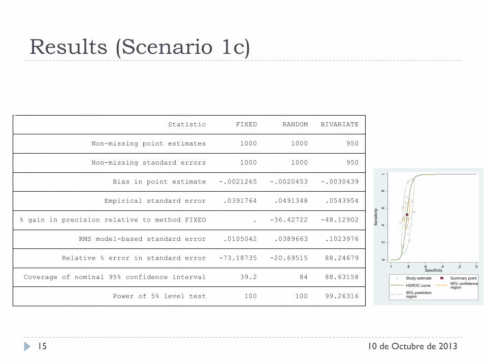
Results (Scenario 1c)


Power of 5% level test 100 100 99.26316 Coverage of nominal 95% confidence interval 39.2 84 88.63158 Relative % error in standard error -73.18735 -20.69515 88.24679 RMS model-based standard error .0105042 .0389663 .1023976 % gain in precision relative to method FIXED . -36.42722 -48.12902 Empirical standard error .0391764 .0491348 .0543954 Bias in point estimate -.0021265 -.0020453 -.0030439 Non-missing standard errors 1000 1000 950 Non-missing point estimates 1000 1000 950 Statistic FIXED RANDOM BIVARIATE

0.2

.4.6

.81

Sen

sitiv

ity






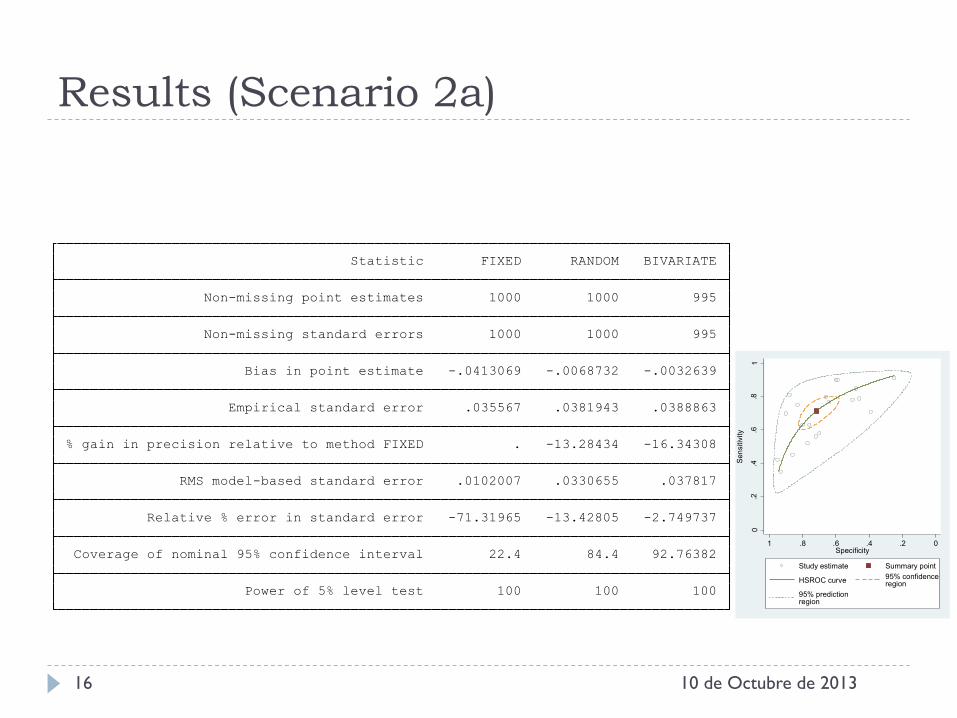
Results (Scenario 2a)

0.2

.4.6

.81

Sen

sitiv

ity





Power of 5% level test 100 100 100 Coverage of nominal 95% confidence interval 22.4 84.4 92.76382 Relative % error in standard error -71.31965 -13.42805 -2.749737 RMS model-based standard error .0102007 .0330655 .037817 % gain in precision relative to method FIXED . -13.28434 -16.34308 Empirical standard error .035567 .0381943 .0388863 Bias in point estimate -.0413069 -.0068732 -.0032639 Non-missing standard errors 1000 1000 995 Non-missing point estimates 1000 1000 995 Statistic FIXED RANDOM BIVARIATE

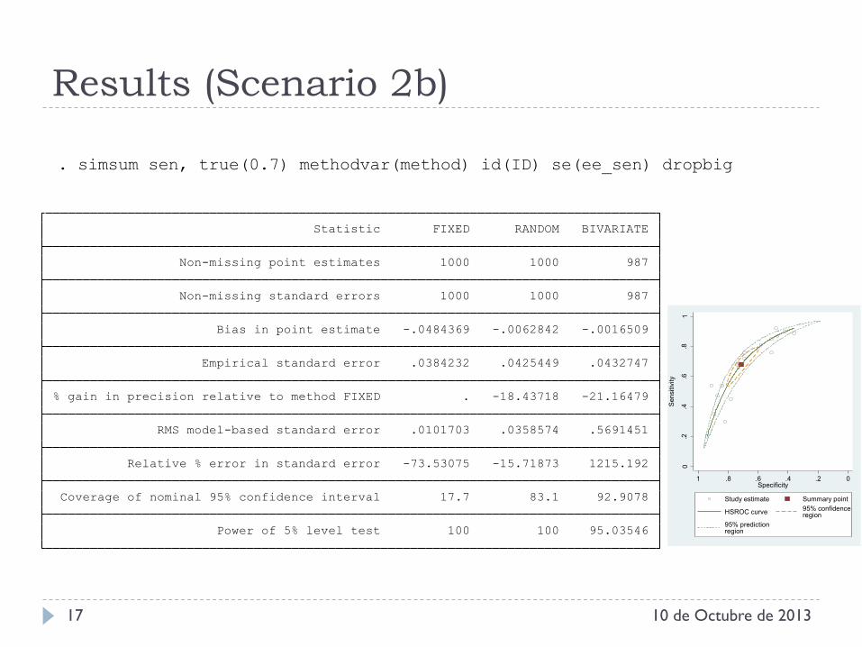
Results (Scenario 2b)

. simsum sen, true(0.7) methodvar(method) id(ID) se(ee_sen) dropbig

Power of 5% level test 100 100 95.03546 Coverage of nominal 95% confidence interval 17.7 83.1 92.9078 Relative % error in standard error -73.53075 -15.71873 1215.192 RMS model-based standard error .0101703 .0358574 .5691451 % gain in precision relative to method FIXED . -18.43718 -21.16479 Empirical standard error .0384232 .0425449 .0432747 Bias in point estimate -.0484369 -.0062842 -.0016509 Non-missing standard errors 1000 1000 987 Non-missing point estimates 1000 1000 987 Statistic FIXED RANDOM BIVARIATE


0.2

.4.6

.81

Sen

sitiv

ity





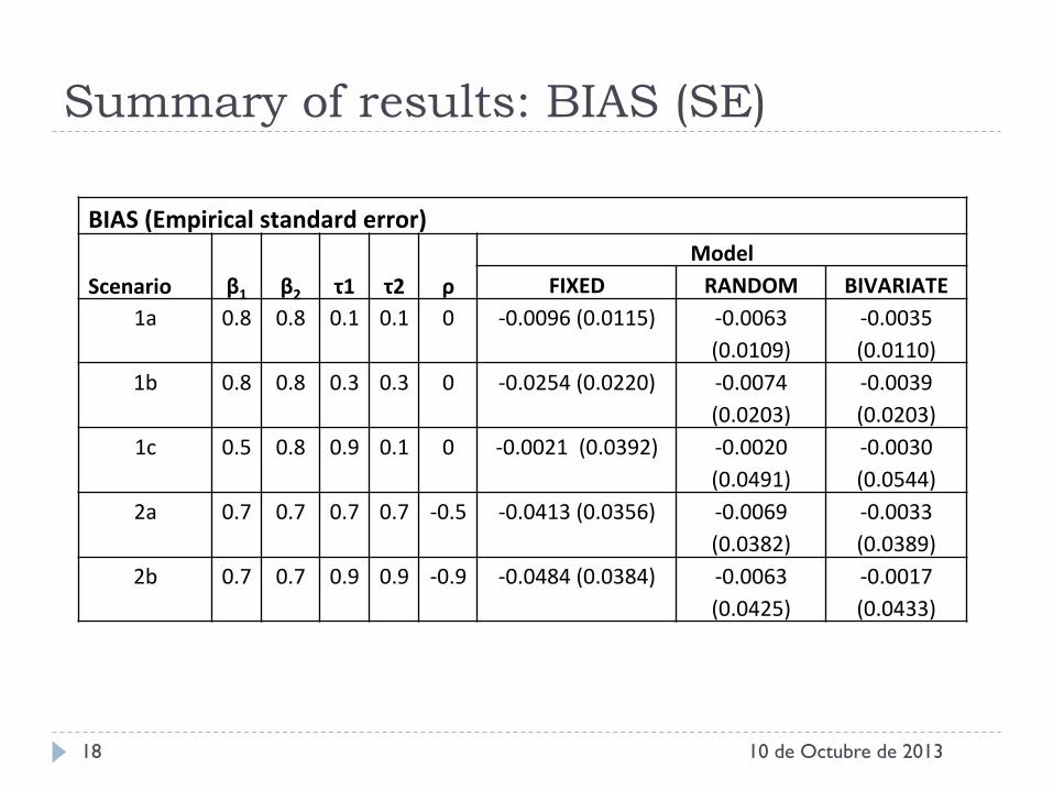
Summary of results: BIAS (SE)


BIAS (Empirical standard error)

Scenario β1 β2 τ1 τ2 ρ Model

FIXED RANDOM BIVARIATE 1a 0.8 0.8 0.1 0.1 0 -‐0.0096 (0.0115) -‐0.0063

(0.0109) -‐0.0035 (0.0110)

1b 0.8 0.8 0.3 0.3 0 -‐0.0254 (0.0220) -‐0.0074 (0.0203)

-‐0.0039 (0.0203)

1c 0.5 0.8 0.9 0.1 0 -‐0.0021 (0.0392) -‐0.0020 (0.0491)

-‐0.0030 (0.0544)

2a 0.7 0.7 0.7 0.7 -‐0.5 -‐0.0413 (0.0356) -‐0.0069 (0.0382)

-‐0.0033 (0.0389)

2b 0.7 0.7 0.9 0.9 -‐0.9 -‐0.0484 (0.0384) -‐0.0063 (0.0425)

-‐0.0017 (0.0433)


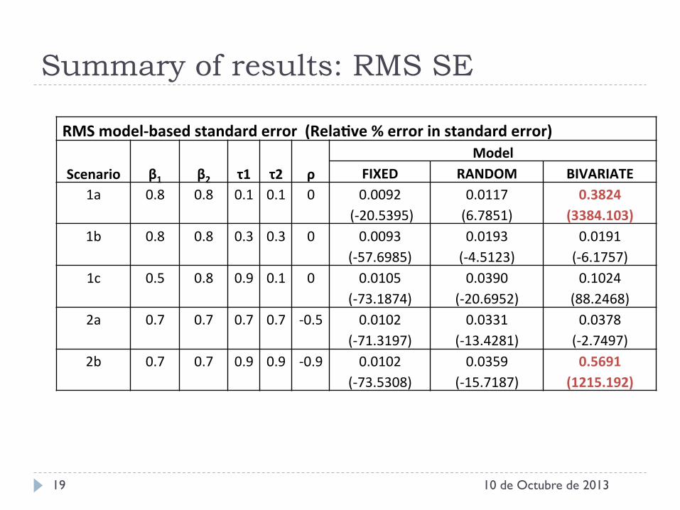
Summary of results: RMS SE

RMS model-‐based standard error (RelaQve % error in standard error)

Scenario β1 β2 τ1 τ2 ρ Model

FIXED RANDOM BIVARIATE 1a 0.8 0.8 0.1 0.1 0 0.0092

(-‐20.5395) 0.0117 (6.7851)

0.3824 (3384.103)

1b 0.8 0.8 0.3 0.3 0 0.0093 (-‐57.6985)

0.0193 (-‐4.5123)

0.0191 (-‐6.1757)

1c 0.5 0.8 0.9 0.1 0 0.0105 (-‐73.1874)

0.0390 (-‐20.6952)

0.1024 (88.2468)

2a 0.7 0.7 0.7 0.7 -‐0.5 0.0102 (-‐71.3197)

0.0331 (-‐13.4281)

0.0378 (-‐2.7497)

2b 0.7 0.7 0.9 0.9 -‐0.9 0.0102 (-‐73.5308)

0.0359 (-‐15.7187)

0.5691 (1215.192)


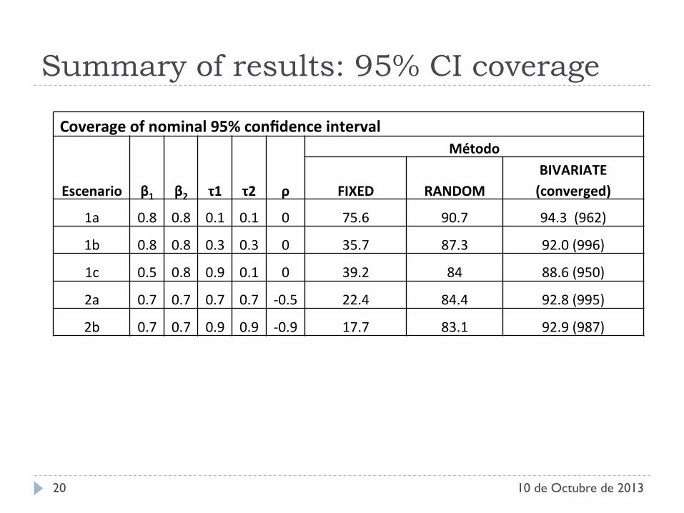
Summary of results: 95% CI coverage

Coverage of nominal 95% confidence interval

Escenario β1 β2 τ1 τ2 ρ

Método

FIXED RANDOM BIVARIATE (converged)

1a 0.8 0.8 0.1 0.1 0 75.6 90.7 94.3 (962)

1b 0.8 0.8 0.3 0.3 0 35.7 87.3 92.0 (996)

1c 0.5 0.8 0.9 0.1 0 39.2 84 88.6 (950)

2a 0.7 0.7 0.7 0.7 -‐0.5 22.4 84.4 92.8 (995)

2b 0.7 0.7 0.9 0.9 -‐0.9 17.7 83.1 92.9 (987)

Conclussions


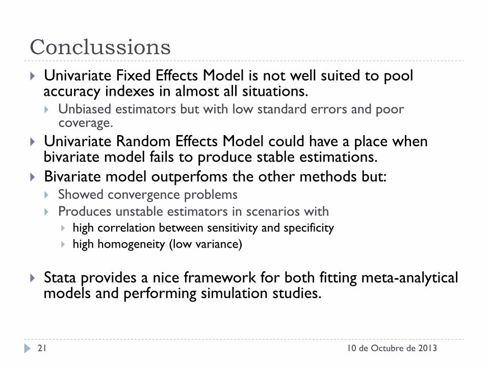
}  Univariate Fixed Effects Model is not well suited to pool accuracy indexes in almost all situations. }  Unbiased estimators but with low standard errors and poor

coverage. }  Univariate Random Effects Model could have a place when

bivariate model fails to produce stable estimations. }  Bivariate model outperfoms the other methods but:

}  Showed convergence problems }  Produces unstable estimators in scenarios with

}  high correlation between sensitivity and specificity }  high homogeneity (low variance)

}  Stata provides a nice framework for both fitting meta-analytical models and performing simulation studies.

Further works


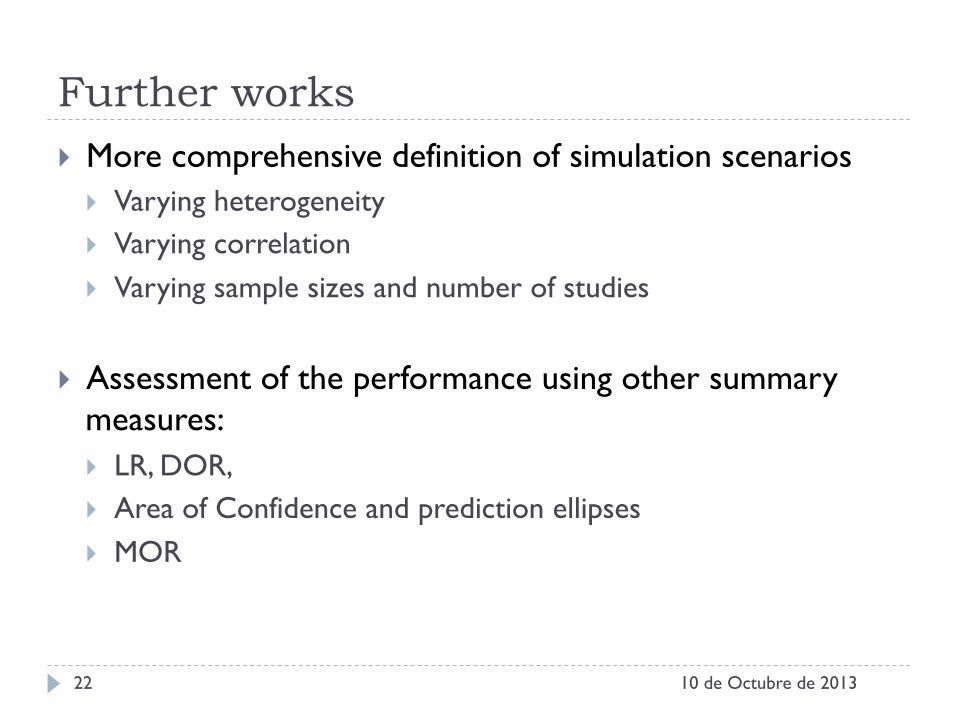
}  More comprehensive definition of simulation scenarios }  Varying heterogeneity }  Varying correlation }  Varying sample sizes and number of studies

}  Assessment of the performance using other summary measures: }  LR, DOR, }  Area of Confidence and prediction ellipses }  MOR

User written commands


}  metan Michael J Bradburn, Jonathan J Deeks, Douglas G Altman. Centre for Statistics in Medicine, University of Oxford, UK }  metandi Roger Harbord, Department of Social Medicine University of Bristol, UK

}  midas Ben A. Dwamena, Division of Nuclear Medicin, Department of Radiology, University of Michigan, USA

}  simsum Ian White, MRC Biostatistics Unit, Cambridge, UK


}  Thank you very much

}  Nieves Plana ([email protected]) }  Víctor Abraira ([email protected]) }  Javier Zamora ([email protected])

Meta-analysis of diagnostic test accuracy studies … of diagnostic test accuracy studies with...

Documents

Transcript of Meta-analysis of diagnostic test accuracy studies … of diagnostic test accuracy studies with...