MESSY TIME SERIES - stat.berkeley.edubrill/Stat248/messyts.pdf104 A. HARVEY S.J, . KOOPMAN, and J....

MESSY TIME SERIES: A UNIFIED APPROACH

Andrew Harvey, Siem Jan Koopman, and

Jeremy Penzer

ABSTRACT

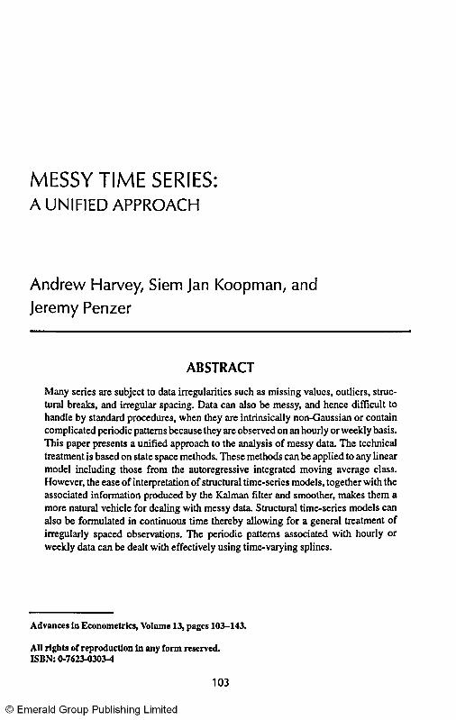
Many series are subject to data irregularities such as missing values, outliers, structural breaks, and irregular spacing. Data can also be messy, and hence difficult to handle by standard procedures, when they are intrinsically non-Gaussian or contain complicated periodic patterns because they are observed on an hourly or weekly basis. This paper presents a unified approach to the analysis of messy data. The technical treatment is based on state space methods. These methods can be applied to any linear model including those from the autoregressive integrated moving average class. However, the ease of interpretation of structural time-series models, together with the associated information produced by the Kalman filter and smoother, makes them a more natural vehicle for dealing with messy data. Structural time-series models can also be formulated in continuous time thereby allowing for a general treatment of irregularly spaced observations. The periodic patterns associated with hourly or weekly data can be dealt with effectively using time-varying splines.

Advances in Econometrics, Volume 13, pages 103-143. Copyright © 1998 by JAI Press Inc. All rights of reproduction in any form reserved. ISBN: 0-7623-0303-4

103

104 A. HARVEY, S.J. KOOPMAN, and J. PENZER

I. INTRODUCTION

The aim of this paper is to examine methods for modeling time series with data irregularities such as missing values, outliers, structural breaks, and irregular spacing. A time series can also be difficult to handle by standard procedures when it contains complicated patterns because it is observed on a weekly or hourly basis. Modeling techniques for these situations are also reviewed. Attention is focussed on univariate time series, though the use of multivariate models in estimating missing values in a series is also discussed.

Autoregressive integrated moving average models are often regarded as providing the main basis for time-series modeling. However, given the technology which is now available, there may be more attractive alternatives particularly when dealing with messy data. The next section sets out the basic ideas of structural time-series modeling and notes the relationship with autogressive integrated moving average models. The Kalman filter is then described. This is needed for handling structural time-series models, but even more important it is crucial for dealing with messy data, irrespective of the class of models used. The remaining sections describe methods for handling a wide range of data irregularities. These methods fall within a unified framework. The reasons for our preference for structural models will become apparent as we proceed.

II. TIME-SERIES MODELS

The basic idea of structural time-series models (STMs) is that they are set up as regression models in which the explanatory variables are functions of time with coefficients which change over time (see Harvey 1989; West and Harrison 1989; and Young 1984). Thus, within a regression framework a simple trend would be modeled in terms of a constant and time with a random disturbance added on, that is

y^OC + Pf + e,, / = 1 T. (1)

The model is easy to estimate using ordinary least squares, but suffers from the disadvantage that the trend is deterministic. In general, this is too restrictive, however, the necessary flexibility is introduced by letting the coefficients a and P evolve over time as stochastic processes. In this way the trend can adapt to underlying changes. The current, or filtered, estimate of the trend is estimated by putting the model in state space form and applying the Kalman filter. Related algorithms are used for making predictions and for smoothing, which means computing the best estimate of the trend at all points in the sample using the full set of observations. The extent to which the parameters are allowed to change is governed by hyperparameters. These can be estimated by maximum likelihood but, again, the key to this is the state space form and the Kalman filter. All these methods

Messy Time Series 105

and algorithms are described in the next section. For applied work the important point is to understand what the models do and how the results should be interpreted. The STAMP package of Koopman and colleagues (1995) carries out all the calculations and is set up so as to leave the user free to concentrate on choosing a suitable model.

The classical approach to time-series modeling is based on the fact that a general model for any indeterministic stationary series is the autoregressive-moving average of order (p, q), that is

yt=VM + • • • + V / - P + ^ + ° I 5 M + • • •+Qfit-q* %t - I ID(°« <#• <*>

where IID(0, a2) denotes independent, identically distributed with mean zero and variance a2. This is usually referred to as ARMA (p,q). The modeling strategy consists of first specifying suitable values ofp and q on the basis of an analysis of the correlogram and other relevant statistics. The model is then estimated, usually under the assumption that the disturbance is Gaussian. The residuals are then examined to see if they appear to be random, and various test statistics are computed. In particular, the BoxrLjung g-statistic, which is based on the first P residual autocorrelations, is used to test for residual serial correlation. Box and Jenkins (1976) refer to these stages as identification, estimation, and diagnostic checking. If the diagnostic checks are satisfactory, the model is ready to be used for forecasting. If they are not, another specification must be tried. Box and Jenkins stressed the role of parsimony in selecting p and q to be small. However, it is sometimes argued, particularly in econometrics, that a less parsimonious pure autoregressive (AR) model is often to be preferred as it is easier to handle. When viewed as approximations to more general ARMA processes, autoregressive models will be written as

yl='*iy,-i+Ttyt-2+•'•+£>,, ^- i iDto.a 2 ; , (3)

Many series are not stationary. In order to handle such situations Box and Jenkins proposed that a series be differenced to make it stationary. After fitting an ARMA model to the differenced series, the corresponding integrated model is used for forecasting. If the series is differenced d times, the overall model is called ARIMA (p, d, q). Seasonal effects can be captured by seasonal differencing.

The model selection methodology for structural models is somewhat different in that there is less emphasis on looking at the correlograms of various transformations of the series in order to get an initial specification. This is not to say that correlograms should never be examined, but our experience is that they can be difficult to interpret without prior knowledge of the nature of the series and in small samples and/or with messy data they can be misleading. Instead the emphasis is on formulating the model in terms of components which knowledge of the application or an inspection of the graph suggests might be present. For example, with monthly observations, one would probably wish to build a seasonal pattern into the model


at the outset and only drop it if it proved to be insignificant. Once a model has been estimated, the same type of diagnostics tests as are used for ARIMA models can be performed on the residuals. In particular the Box-Ljung statistic can be computed with the number of relative hyperparameters subtracted from the number of residual autocorrelations to allow for the loss in degrees of freedom. Standard tests for nonnormality and heteroscedasticity can also be carried out, as can tests of predictive performance in a post-sample period. Plots of residuals should be examined, a point which Box and Jenkins stressed for ARIMA model building. In a structural time-series model such plots can be augmented by graphs of the smoothed components. These can often be very informative since they enable the model builder to check whether the movements in the components correspond to what might be expected on the basis of prior knowledge.

The subsections below set out the principal univariate structural time-series models. The relationship between structural and ARIMA models is then discussed.

A. Local Level

The simplest structural time-series model addresses a situation in which the underlying level of the series changes over time. This level is modeled by a random walk, on top of which is superimposed a random, or white noise, disturbance. The specification is therefore

y, = H, + e r e,~NID(0,o2), / = l , . . . , r , <4>

H ^ l V i + iV Tl,~NID(0,a2), where NID denotes normally and independently distributed, and the two disturbances are mutually uncorrelated. An important practical feature of this model is that the estimator of the level, based on currently available information, is given by an exponentially weighted moving average (EWMA) of past observations where the smoothing constant is a function of the signal-noise ratio, q = G\/G\. Forecasts of future observations, however many steps ahead, are given by exactly the same expression. This was established by Muth (1960). For a pure random walk, q is infinite, leading to a forecast equal to the last observation. As q moves toward 0, the forecast becomes the sample mean.

B. Local Linear Trend

The local linear trend model replaces the deterministic trend in (1) by a stochastic trend. The exact formulation is

y/-M, + e». e,~NID(0,oi), r = l T,

MI-MM + PM + H,. TI,~NID(0,O5),

P, = PM + C,. C-NIDCO.O*), ( 5 )


with the level and slope disturbances, i)t and £,, mutually uncorrected and uncorrected with e r The extent to which the level, n,, and slope, p r change over time is governed by the relative hyperparameters, q^ = o^/a* and q^ = o^/o^. The forecast function is a straight line starting from the estimates of the level and slope at the end of the sample. In the limiting case when both relative hyperparameters are zero, the deterministic trend model is obtained with a = |i0. Other special cases of interest arise when qr = 0, in which case the trend is a random walk plus drift and q~ = 0, in which case the smoothed trend is similar to a cubic spline.

C. Trend, Seasonal, and Irregular

Many series recorded quarterly or monthly are subject to seasonal variation. What is effectively seasonality also occurs when observations are recorded within the day. Just as more flexibility needs to be given to a trend by allowing it to be stochastic, so a seasonal component needs to be allowed to change over time. Although the case for a stochastic seasonal component is arguably less compelling than the case for a stochastic trend, there are many reasons why changes in the seasonal pattern may take place (see Harvey 1989, pp. 95-98).

If the seasonal component is deterministic, it should have the property that it sums to zero over the previous year; this ensures that it cannot be confounded with the trend. Adding a disturbance term to the sum of seasonal effects over the past year allows the seasonal pattern to evolve over time. This is the dummy variable form of stochastic seasonality:

Y, = -YM-----Y,-J+ i+c<V (0,~NID(0,c£). (6)

An alternative way of capturing a deterministic seasonal pattern is by a set of sine and cosine functions. Allowing these to be stochastic leads to the trigonometric form of stochastic seasonality:

Y,-2V (7)

where each v. t is generated by

cos Xy sin Xj

-sin A., cos Ay +

(0 . y = l [s/2].

(8)

where X;. = 2nj/s is frequency, in radians, and u), and (0* are two mutually uncorrected white noise disturbances with zero means and common variance o^ for / = 1 T. For s even [s/2] = s/2, while for s odd, [s/2] = (s-l)/2. For s even, the component at/ = s/2 collapses to


Wi^V^ j=s/z (9)

Without the disturbance terms this seasonal model will give the same deterministic pattern as the dummy variable seasonal model. However, it is a better model of stochastic seasonality because it allows the seasonal pattern to evolve more smoothly; it can be shown that the sum of the seasonals over the past year follows an M A ( J - 2 ) rather than white noise.

Seasonal effects are typically combined with trend and irregular components, usually after taking logarithms. This leads to the basic structural model (BSM). It may be written as

v, = H, + Y, + er f = l T, (10)

where the stochastic trend component, ^ and the irregular component are defined as in the local linear trend model above.

D. Cycle

A deterministic cycle can be expressed as a sine-cosine wave, that is

y, = acosX/ + |3sinX/, / = 1 T. (11)

In the previous section it was pointed out that a seasonal pattern could be modeled by a set of such cycles defined at the seasonal frequencies. Adding disturbances allowed the pattern to change over time. A somewhat different situation arises when we wish to model a cycle, which may be stochastic, and, unlike the seasonal cycles may be stationary. The statistical specification of such a cycle, \ j / r is as follows

= P

-cosXc sinXc

-+

K/

-sinXc cosXc < I < /=i r, (12)

where Xc is the frequency, in radians, in the range 0 <, Xc <i n, K, and K* are two mutually uncorrected white noise disturbances with zero means and common variance a*, and p is a damping factor, such that 0 < p £ 1. Note that the period is 2n/Xc. For some purposes it is useful to take the variance of ^ rather than the variance of KP as a hyperparameter. Then since o j = (1 - p2) oL a deterministic, but stationary, cycle is obtained when p = 1. The ACF of \yt is

p(t) = pT cos XT, T = 0 , 1, (13)

This is a cycle which damps down to zero as x goes to infinity, except when p = 1. The spectrum has a peak around Xc, denoting irregular, or pseudo-cyclical, behavior. The peak becomes sharper as p approaches one and in the limiting case when p equals one it manifests itself as a jump in the spectral distribution function. A test


of the hypothesis that p = 1 against the alternative that it is less than one is given in Harvey and Streibel (1998).

Cyclical components of this type have proved useful in economics for modeling the business cycle, and in meteorology for modeling rainfall (see Harvey and Jaeger 1993; Koopman et al. 1995). Cyclical components can be combined with other components, such as trend and seasonal, as well as with other cycles or perhaps autoregressive processes. An AR(1) process is actually a limiting case of the stochastic cycle when Xc is 0 or ft, though it is usually specified separately, partly to avoid confounding and partly because it is not a limiting case in multivariate models.

E. Reduced form ARIMA Models

All the structural time-series models described in the previous section are linear and hence there is a corresponding ARIMA model which gives identical predictions. Since the ARIMA model contains only a single disturbance, it is called the reduced form.

The specification of the reduced form can be found very easily for the simpler models. Thus for the local level, (4), taking first differences yields

A>v = Ti, + e , - e M , r = 2 , . . . , r . (14)

The first order autocorrelation is -1/(2 + q), while the remaining higher order autocorrelations are all zero. Hence the ACF is the same as that of an M A( 1) process and so the local level has an ARIMA(0,1,1) reduced form, that is

Ay, = £, + e£ M , f = 2 T. (15)

Equating the first order autocorrelations in the two models gives the following relationship between the structural and reduced form parameters:

Q = [(q2 + 4)l/2-2-q]/2. (16)

In the ARIMA(0,1,1) reduced form, 0 is constrained to be negative. In more complicated models the constraints tend to be stronger. For example, the reduced form of a model consisting of stochastic trend, cycle, seasonal, and irregular components is an ARIMA model in which the observations follow an A R M A ( 2 , J + 4) process after first and seasonal differencing, that is AA5 yt ~ ARMA(2, s + 4). If it were not subject to restrictions, such a process would contain considerably more parameters than the structural form. Indeed, an ARIMA model of this complexity would virtually never be identified and if it were it would probably prove impossible to estimate.

The BSM has a reduced form which, as shown in Maravall (1985), is quite close to that of the ubiquitous airline model of Box-Jenkins analysis, namely the seasonal ARIMA of order (0,1,1) x (0,1,1),:

no A. HARVEY, S.J. KOOPMAN, and J. PENZER

AA,y, = (l + eL) ( l+GL%, ^-NID(0,o2). (17)

In fact the special case of the BSM when the seasonal and slope disturbance variances are equal to zero is equivalent to an airline model with a seasonal moving average parameter, G, equal to minus one.

Autoregressive models can be poor approximations when components are slowly changing. For example, in the local level model a small value of q corresponds to a value of 0 close to -1 and the coefficients in the autoregressive representation of Ay,, which are equal to -(-8)-', die away very slowly. When a seasonal component is present, it will typically change slowly relative to the rest of the series with the result that an AR approximation can be very poor (see Harvey and Scott 1994).

F. Explanatory Variables

Explanatory variables can easily be included in a structural model. In later sections we make extensive use of explanatory variables which are dummy variables. These are used to handle missing observations and intervention effects. If xt is a k X 1 vector of observed explanatory variables and P is a corresponding vector of parameters, the model

y, = u., + *;p+Er, /=!,...,r, (18)

2

1.9

1.8

1.7

1.6

U

1.4

1.3

1870 1880 1890 1900 1910 1920 1930 1940

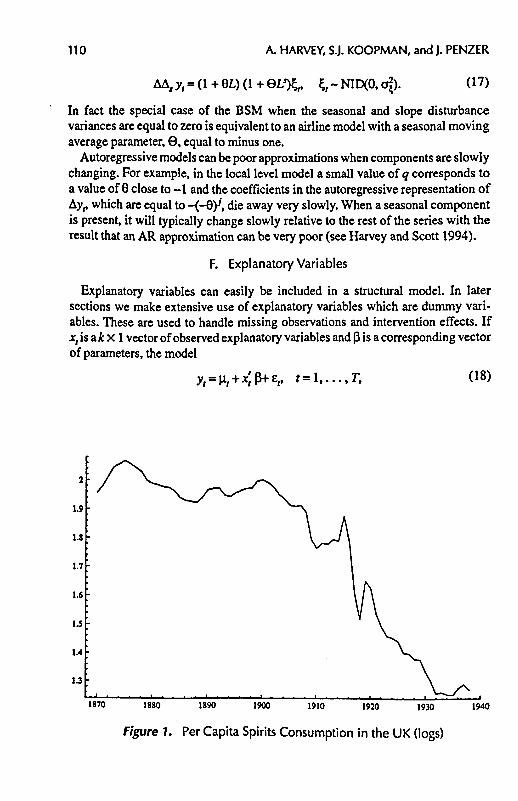
Figure 1. Per Capita Spirits Consumption in the UK (logs)


•prict I

2.4

2 J2\

1870 1880 1890 1900 1910 1920 1930 19

2,1

2

" | incoroa 3 2,1

2

;

1.9

1.8 • . . . . i

1870 1880 1890 1900 1910 1920 1930 1940

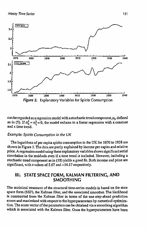
Figure 2. Explanatory Variables for Spirits Consumption

can be regarded as a regression model with a stochastic trend component, \it, defined as in (5). If a^ = al = 0, the model reduces to a linear regression with a constant and a time trend.

Example: Spirits Consumption in the UK

The logarithms of per capita spirits consumption in the UK for 1870 to 1938 are shown in Figure 1. The data are partly explained by income per capita and relative price. A regression model using these explanatory variables shows significant serial correlation in the residuals even if a time trend is included. However, including a stochastic trend component as in (18) yields a good fit. Both income and price are significant, with /-values of 5.67 and -14.17 respectively.

III. STATE SPACE FORM, KALMAN FILTERING, AND SMOOTHING

The statistical treatment of the structural time-series models is based on the state space form (SSF), the Kalman filter, and the associated smoother. The likelihood is constructed from the Kalman filter in terms of the one-step-ahead prediction errors and maximized with respect to the hyperparameters by numerical optimization. The score vector of the parameters can be obtained via a smoothing algorithm which is associated with the Kalman filter. Once the hyperparameters have been


estimated, the filter is used to produce one-step-ahead prediction residuals which enables us to compute diagnostic statistics for normality, serial correlation, and goodness of fit. The smoother is used to estimate unobserved components, such as trends and seasonals, and to compute diagnostic statistics for detecting outliers and structural breaks. ARIMA models can also be handled using the Kalman filter. The state space approach becomes particularly attractive when the data are subject to missing values or temporal aggregation.

A. State Space Form

All linear time-series models have a state space representation. This representation relates the disturbance vector {e,} to the observation vector {yt} via a Markov process {a,}. A convenient expression of the state space form is

y, = Z,a, + G,e,, (19)

a,+i = r,cx, + //,e,, t=l 7, (20)

where a, is the m x 1 state vector, e, is a k x 1 vector of disturbances and the system matrices Z,, Tr G,, and Ht have dimensions l x m , l x / : , mxm, and mxk, respectively. The disturbances are mutually uncorrelated white noise variables with mean zero and unit variance. When we assume Gaussianity, they are also independent of each other. The appearance of the disturbance vector e, in the measurement equation (19) and in the transition equation (20) is general rather than restrictive. The system matrices G, and Ht can be interpreted as selection matrices. For example, uncorre-latedness of the measurement and transition disturbances is the special case //,Gj = 0, for t = 1 , . . . , T. The system matrices Z,, Tr G r and H, are fixed and their unknown elements, if any, are placed in the hyperparameter vector \j/ which can be estimated by maximum likelihood. In univariate time-series models, Zt and Gt are row vectors and Gfft is a scalar.

The initial state vector a t is assumed to be random with mean a and variance matrix P where a and P are known. If a, is nonstationary then a is thought of as having a diffuse prior, that is the variance matrix P is set equal to K/, where K is a scalar which tends to infinity (see Harvey 1989).

B. Kalman Filter

In the Gaussian state space model the Kalman filter evaluates the minimum mean squared estimator of the state vector at+l using the set of observations ^»= tvi, • • • • y,}» denoted a/+1 = £(a,+llY(), and the corresponding variance matrix P,+l = Vai(a,+1iy,), for t = 1 T. The Kalman filter is given by


Kt = (JtPtZ't + Ht(?t) FJl (21) flm-^A + *ivr P<+l = TAL't + HtJ't, f = l T,

where Lt = Tt- K, Z,, J, = Ht- Kt Gt and with the initializations a, = a and fj = P. The derivation of the Kalman recursions can be found in Anderson and Moore (1979) and Harvey (1989). The limiting case P = K/, where K -» «>, can be handled using a relatively straightforward modification of the Kalman filter as proposed by Ansley and Kohn (1985,1990) and developed further by Koopman (1997). Other treatments of the limiting case are given by de Jong (1991) and Snyder and Saligari (1996). The one-step-ahead prediction error of the observation vector is v, = yt - is(yrIK,_j) with covariance matrix Ft = Var(y,IKM) = Var(v,). The output of the Kalman filter is used to compute the log-likelihood function /(y; \y), conditional on the hyperparameter vector \|/, as given by

T T (22)

/(y;v)=-fiog27t-i2I°glf,/l-lEv;Fr1v/, 1=1 M

apart from a constant. Numerical maximization of /(y; \y) with respect to the hyperparameter vector \j/, yields the maximum likelihood estimator y/.

C. Smoothing

The work of de Jong (1988, 1989), Kohn and Ansley (1989), and Koopman (1993) leads to a smoothing algorithm from which different estimators can be computed based on the full sample Yr Smoothing takes the form of a backward recursion,

ut = F-xvrK'trt, Ml = FJl + K'lNtKr r = r , . . . , l ,

r M = Z , V 7 > r N_x=Z'tF;% + L'tNtLt, (23)

where rT = 0 and NT = 0. The recursions require memory space for storing the Kalman output v,, Ft and Kv for f = 1 , . . . , T. The series {u,} will be referred to as smoothing errors. As we will see later, the smoothing quantities ut and rt play a pivotal role in the construction of diagnostic tests for outliers and structural breaks. The smoother can be used to compute the smoothed estimator of the disturbance vector e, = E(Et\YT), that is

e, = G;W/ + «;r,, V a r v e ^ G ^ G j + . / ^ y , , i - r . . . . . l . <24>

for any [G,] and {//,} (see Koopman 1993). The smoothed estimator of the state vector a, = E(at\Yj) is constructed via the simple forward recursion


A mmm A _ _ A

/= i , . . . , r , (25)

where ax = a + Pr0. A more elaborate algorithm for computing the smoothed state vector, including the evaluation of its covariance matrix, is given by de Jong (1988, 1989) and Kohn and Ansley (1989). Finally, the output of the smoother can also be used to compute the exact score for hyperparameters (see Koopman and Shephard 1992). For example, the score of \jf,., that is the ith element of the hyperparameter vector \jf which only relates to entries in {Ht} and [Gt], is given by

(26) 3/(y;y) oG, ., „ % on, .

The evaluation of (26) only relies on the smoothing recursion (23).

D. State Space Form for Structural Models

The random walk plus noise model is essentially in state space form as it stands. Since e,andr|r are uncorrelated in all time periods, the fact that the transition equation is shifted forward in time in (20) is not important so Z, = T, = 1, G, = (o, 0), and Ht - (0 on). For the local linear trend model the state vector is now of length two. We still have a time invariant representation, Z ^ - ( 1 0 ) i C l - ( o t 0 0 ) i

7>fi !l and '41) f° °"n 0^ H,= 1

t 0 0 o> 0 0 o>

Other structural models can easily be put in state space form (see Harvey 1989).

E. State Space Form of ARIMA Models

A state space representation for ARMA models was suggested by Akaike (1974). We adopt the representation put forward by Pearlman (1980) in which the state vector is of length r = max(p, q). For a general univariate ARMA(p,q) process the state space quantities in (19) and (20) take the form

r=

Z=(l 0 . . .0) . G = 1.

'•i 1 0 . . 0> v^r <>2 0 %. •

. 1 , H =

<t>2+e2

*, o ... . .. 0 fc+e.

(27)


Note that in this representation both measurement and transition noise are given by univariate e,, the ARMA error term. Nonstationary AR1MA(p,d,q) processes can be put in state space form by augmenting the state vector as in Harvey and Pierse (1984). If a* is the augmented state vector,

a.

yt-i

where yli=(y(.{ • y,_d)'. The Markovian representation of the series is

y/ = (Z8,- . .8 < i )a ; + ep

<Vi =

V o <f 'it Z 8* 8, «;+ i

0 AM 0 \ J

0

(28)

where 8y = (-l^dl/jltf - ; ) ! , 8* = (5, • • • 8^,) and T, Z and H are given by (27). If the first d members of the series are observed, the filtering recursions can be initialized at t = d + 1 using

*</+! =

where Px = Eict^).

V *v J

and r«/+i o o

IV. MISSING OBSERVATIONS AND TEMPORAL AGGREGATION

The mechanism for observing time-series is often imperfect. Equipment failure, human error, or the disregarding of inaccurate measurements can introduce missing values. Nature does not always provide a complete data set, for example, measurement of the concentration of pollutants in rainfall is impossible if it does not rain. In this section we describe some techniques for dealing with missing values such as modifying the Kalman filter or using dummy variables. We go on to show how state space techniques can be adapted to deal with the related problems of temporal and contemporaneous aggregation.

Missing values arise when there is no information about a stock variable, for example the money supply, at a particular point in time. When the variable in question is a flow, such as income, it is possible that failure to observe it at time t-k leads to our observing its accumulation at / = k +1. This is known as temporal aggregation.


An example of mixed frequency data is any series which is now recorded every quarter but was originally only available on an annual basis. More generally, mixed frequency data arise when the time intervals between observations are not constant. The problem can be dealt with using the irregularly spaced observation approach described in subsection IV.B or by formulating the model in continuous time (see, for example, Harvey and Stock 1993).

A. Missing Observations in Stock Variables

The Kalman filter provides a general tool for handling missing observations. When a missing observation is encountered at t = x, the filter simply skips the updating part of equation (21). This can be interpreted as treating the missing observation yx as a random variable with infinite variance so that Gx —> °°. In the Kalman filter step at time t = x the Kalman gain, is Kx equal to zero and

at+l = Txax> Px+1 = TxPxTx + HxHx •

There is no prediction error at t = X. The smoothing equations (23) at time t = x, reduce to

rx-i = Txrx> ^ r W r

with ux = 0 and Mx = 0. The value taken by the process at points where no observation is made may be of interest. The minimum mean square estimate of yx is given by

A A

yx=zx<*v

where cct is obtained from (25). The likelihood can be evaluated using (22) where the summations are now only made over the prediction errors corresponding to values which are observed.

If a model contains d stationary components, the first (or last) d values of the series can be used to construct initial conditions for the filter. Situations arise in practice in which both the first and the last d members of the series contain missing values. This is particularly true for seasonal models in which the number of nonstationary components is large. This problem can be overcome by using a diffuse initialization for the filter as discussed in subsection IIIB.

A missing observation can also be handled by introducing a dummy variable into the measurement equation (19), that is

y, = Z,a, + AJc, + e,, r = l 7,

where xt is an indicator variable which is equal to zero for all time periods except at time t = x where it is unity. It should be noted that the state space framework can be extended to include explanatory variables. Given the hyperparameters, introducing a dummy variable has exactly the same effect as skipping a filter update as


described above (see Harvey 1989, p. 145). If the hyperparameters are unknown, a correction must be applied to the determinantal term of the likelihood function (Sargan and Drettakis 1974). However, when A is included in the state vector and the element of the initial state vector associated with A. is treated as a diffuse random variable, the likelihood function computed by the exact initial Kalman filter is corrected automatically. This approach is easily generalized to multiple missing observations.

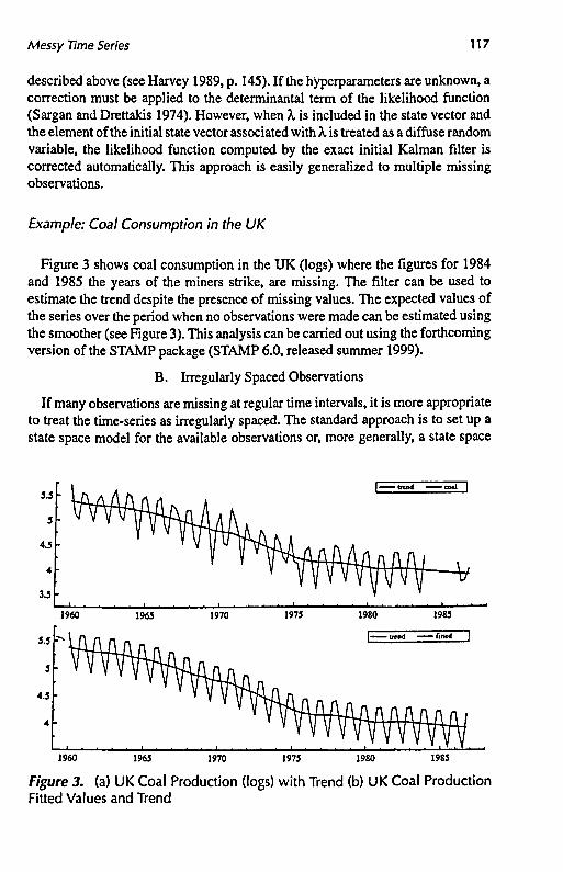
Example: Coal Consumption in the UK

Figure 3 shows coal consumption in the UK (logs) where the figures for 1984 and 1985 the years of the miners strike, are missing. The filter can be used to estimate the trend despite the presence of missing values. The expected values of the series over the period when no observations were made can be estimated using the smoother (see Figure 3). This analysis can be carried out using the forthcoming version of the STAMP package (STAMP 6.0, released summer 1999).

B. Irregularly Spaced Observations

If many observations are missing at regular time intervals, it is more appropriate to treat the time-series as irregularly spaced. The standard approach is to set up a state space model for the available observations or, more generally, a state space

| - ^ t r e n d — c o « l |

?60 1965 1970 1973 1980 1983

1960 1963 1970 1973 1980 1985

Figure 3. (a) UK Coal Production (logs) with Trend (b) UK Coal Production Fitted Values and Trend

118

lr

A. HARVEY, SJ. KOOPMAN, and J. PENZER

I—"-" I

F ^ r

1 2 3 4 5

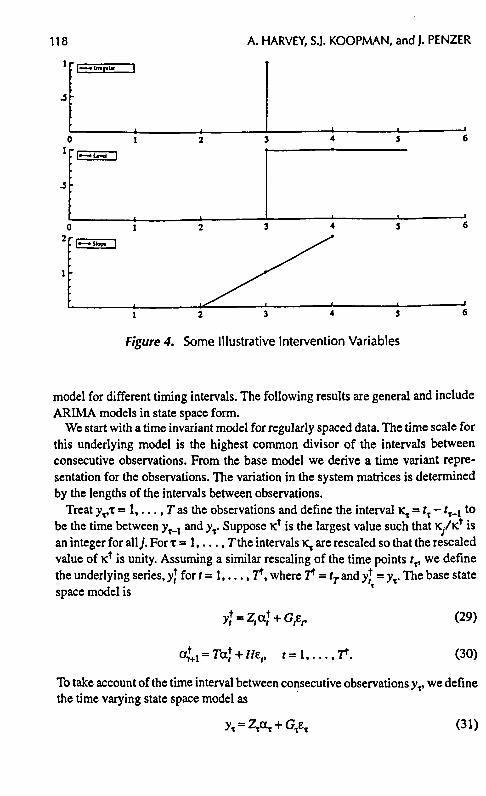
Figure 4. Some Illustrative Intervention Variables

model for different timing intervals. The following results are general and include ARIMA models in state space form.

We start with a time invariant model for regularly spaced data. The time scale for this underlying model is the highest common divisor of the intervals between consecutive observations. From the base model we derive a time variant representation for the observations. The variation in the system matrices is determined by the lengths of the intervals between observations.

Treat yvx = 1 , . . . , T as the observations and define the interval K, = fT - fT_i to be the time between yx-l and yt. Suppose K* is the largest value such that KJ/K* is an integer for all;. For x = 1 , . . . , 7the intervals Kt are rescaled so that the rescaled value of K* is unity. Assuming a similar rescaling of the time points tv we define the underlying series, y) for t = 1 , . . . , 7*, where 7* = tT and y) = yx. The base state space model is

c£1 = 7,a,t + //e,, /=1 7*.

(29)

(30)

To take account of the time interval between consecutive observations yx, we define the time varying state space model as

y t = ZtaT + GTeT (31)


CCT+i = 7 ^ + 11,, x = l , . . . ,T (32)

where

Tx = T\r\x = ̂ TKrJHex and Var(Tit) = £ TKrJ H fT (j'fJ.

This approach is only efficient when the state transition matrix operations for the base model are computationally expensive. Otherwise, it is more straightforward to use the base model and to treat observations not occurring within the time interval K as missing. The latter option clearly applies to structural time-series models. An alternative way of proceeding is to set up the model in continuous time as in Harvey (1989, Chap. 9) and Harvey and Stock (1993).

C. Temporal Aggregation

When dealing with temporal aggregation, we distinguish between the regularly spaced underlying series, y),t= 1 , . . . ,7*, and the observed series, yvT= 1 , . . . , r, which consists of aggregates of yj. Assuming aggregates are observed every K time periods, the aggregated series can be written as

yi = E^(T-iH' T = 1 T' M

An augmented state space approach is used to deal with aggregation. For an ARMA model with a representation as in (27), the state vector for this representation is

«/ = a. V M

where a,is the state vector for the state space representation of the underlying series, >V_i = (y;_j • • • ^JLK+I)'- The measurement and transition equations are

yt = (Z, /)a; + G,e,, t = KT, T = 1 , . . . . 7,

(T.

«/+ i =

K-2

a; + 0

(33)

where we treat yt as missing for f * KT and i is a (K-l) vector of ones. In the ARIMA(p, d, q) case, we have an augmented model for the underlying

series (28). Aggregation can be represented by adapting the measurement equation (Harvey and Pierse 1984). For example, if K - 1 £ d then taking


y/ = (Z,81 + 1...5K_1 + 1 5 K . . . 5 X + e r

yields an observed series consisting of aggregates of the underlying ARIMA process.

For a structural model no transformations such as differencing need to be applied to the observations. Hence temporal aggregation can be handled by means of cummulator variable,

r

>KT+/+1 = 2J y»c(T-I)+i+l» r = l . - - - t K , T = l , . . . , i .

When r = K, this gives the observations which, for reasons of initialization in the state space form of (19) and (20), have to be dated at t = K + 1, 2K + 1 , . . . , with all of the other y's, including yv being treated as missing. The state space form is

y, = ( 0 1 ) a , , / = l , 2 ,

a , + i T 0

zr v, a.

A (R 0 \ZR 1

n,

^ 7+1

with y, = 0 for t =s K, 2K, 3K, . . . . and 1 otherwise.

D. Contemporaneous Aggregation

In multivariate processes we may observe aggregation across series. For example, each series may represent sales of a single good and at some time points only aggregated sales figures are available. This can be dealt with by a simple adaptation of the measurement equation for the underlying N dimensional process, y*= fyi * *' ytjtf- S uPP° s e mat» a t &me '» onty m e aggregate y* = Zj^ ytj is observed. The measurement equation is then

y ;=z ;a ,+G;e ,

where Z* = iZr G* = i Gt and / is an N x 1 vector of ones. This idea can clearly be extended to any pattern of aggregation across series.

V. OUTLIERS AND STRUCTURAL BREAKS

In this section we discuss ways of testing for outliers and structural breaks, and distinguishing between them. We present general procedures, based on the SSF, for calculating the required statistics. These algorithms are exact and can be used within an ARIMA as well as a structural time-series framework. However, as we argue in


the final section, there are considerable advantages to adopting an approach based on the latter.

An outlier is an observation which is not consistent with a model which is thought to be appropriate for the overwhelming majority of the observations. It can be captured by a dummy explanatory variable, known as an impulse intervention variable, which takes the value one at the time of the outlier and zero elsewhere.

A structural break occurs when the level of the series shifts up or down, usually because of some specific event. It is modeled by a step intervention variable which is zero before the event and one after. A structural break in the slope can be modeled by a staircase intervention which is a trend variable taking the values, 1 ,2 ,3 , . . . , starting in the period after the break.

The concepts of outliers and structural breaks apply quite generally. However, it is helpful for what follows to note that the level and slope breaks can be viewed in terms of impulse interventions applied to the level and slope equations of the local linear trend model (5). The structural framework also suggests that it may sometimes be more natural to think of an outlier as an unusually large value for the irregular disturbance. This leads to the notion of a level shift arising from an unusually large value of the level disturbance while a slope break can be thought of as a large disturbance to the slope component. Thus, interventions can be seen as fixed or random effects. However, the random effects approach is more flexible. For example, introducing an outlier intervention at t = T is equivalent to regarding the irregular variance at this point as being infinite. By using a large finite variance, we can ensure that the observation yT is downweighted without being removed altogether.

Viewing intervention effects as random is consistent with the representation of the stochastic trend in (5). In this model the level and slope components are subject to random shocks at each point in time. When such movements are abnormally large, increasing the variance of the relevant disturbance or including an intervention variable may be appropriate.

Example: U.S. CNP

Figure 5 shows the log of U.S. GNP from the first quarter of 1951 to the last quarter of 1985. Placing slope interventions, somewhat arbitrarily, in 1960 quarter 1 and 1970 quarter 1 leads to a model with a deterministic trend as illustrated in figure 5b. There is now a sizeable literature in econometrics on such piecewise linear trends (see the review by Stock 1994). However, unless there is prior knowledge of where the break takes place, it is inadvisable to start off by fitting a piecewise linear trend. A stochastic trend is flexible enough to adapt to breaks, if they are present, and will give an indication of where such breaks occur. Figure 5a shows a stochastic trend fitted to the U.S. GNP data in the absence of any interventions.


-4.6

50 55 60 65 70 75 80 85

-4.2 -

•4.4

•4.6 '

SO 55 60 65 70 75 80 85

Figure 5. (a) U.S. GNP (logs) with Stochastic Trend (b) U.S. CNP (logs) with Deterministic Trend Having Fitted Two Slope Interventions

A. Detection of Outliers

Testing for Outliers Using Impulse Variables

Suppose that we want to test for an outlier at time t = x. If an outlier were present the model could be written

yt = \jct + *V ' = ! . • • - .7\ (34)

where xt is a dummy variable which takes the value one at t = x and is zero elsewhere, Xt is a parameter and wt is generated by a linear time-series model. This could be an STM, an ARIMA model, or even a model which is not time invariant. Written in matrix terms (34) becomes

y = x\ + w, E(w) = 0, Var(w) = o2 V, (35)

where x is a Tx 1 vector which has one in the tth position and is zero everywhere else. Note that (34) was introduced in Section IVA to handle missing observations.

If the model is nonstationary, the above formulation assumes fixed initial conditions. The results also apply when the initial conditions are diffuse and indeed this is the case in which we are primarily interested. However (35) is easier to deal with for expositional purposes.


The hyperparameters appear in the Tx T matrix V. Assuming they are known, the GLS estimator of XT is

jLx = *V~ly/*V~lx, (36)

while

Var(Xt) = o2/jc'V-1x.

A /-test for the significance of the outlier is then constructed as

r = j c T V ^ ? T ^ (37)

where a2 is the unbiased estimator of a2. If the hyperparameters are estimated, then t is asymptotically normal and it can be interpreted as a Lagrange multipler (LM) test.

The construction and inversion of the V matrix can be avoided by putting the model in SSF and applying the smoothing algorithm set out in equation (23). In univariate models it is convenient to set up the state space form in such a way that the KFS can be run independently of a2. In this case, Var(w,) = a2mt and Var(v,) = o 2 / r these quantities being given by Mt and Ft respectively in (23) and (21). The r-statistic in (37) is then given by the standardized smoothing errors that is

B.-n/ f tm}' 2 . x = l T. (38)

(see de Jong 1989; de Jong and Penzer 1998). Indeed the algorithm gives these quantities for all time periods so only one pass is needed to produce the statistics for testing for an outlier at any point in the sample.

For future reference we will let u denote the Tx 1 vector with rth element ur so that

u = Vly. (39)

Note that, if L denotes the lower triangular matrix in the Cholesky decomposition, V"1 = V F~lL, where F is a diagonal matrix with rth elements Ft as in (21), then the Tx 1 vector of innovations in the Kalman filter is given by v = Ly. Hence

u = L'F-lv, (40)

Thus ut depends on current and future innovations, a feature which is also apparent from the KFS (21).

If wt has an autoregressive representation (possibly with unit roots) an explicit expression can be given for an estimator of Xr Carrying out the computations in this way is the standard approach used in the ARIMA based literature on additive outliers (Fox 1972; Tsay 1986, 1988; Chang, Tiao, and Chen 1988). Let


n(L) s l - T t j L - J i j L 2 - . . . such that rc(L)w, = £, where ̂ is a white noise process with mean zero and variance o?. The assumption is then that (34) can be written

7l(L)y, = Xt7l(L)x, + S,, / = l , . . . , r . (41)

This is an approximation insofar as pre-sample observations must be set to zero. The GLS estimator of \ is obtained by applying OLS to (41) to give

\ = S7t;7l(LK+;/nr-f *=l , . . . , r , <42>

where

It can be seen that the expression for XT depends on current and future values of the prediction errors from the AR representation, n(L)yt\ compare (40).

The fact that observations are not available beyond / = T means that (42) may be a poor approximation to (36) if T is located toward the end of the sample. How close (42) is to (36) depends on the process generating wr For example if it is AR(1) then (42) is exactly equal to (36) for any 1 < T < T. However, if wt is a random walk plus noise, as in (4), then

7t(L) = i - ( i - e ) L + e ( i - e ) L 2 - e 2 ( i - e ) L 3 + ..., and it can be seen that these weights will die away very slowly if q is small so that 6 is close to minus one.

If x is located in the middle of a doubly infinite sample we obtain

Xt = 71(F) 71 (ZOy/II.. (43)

where F = LTl is the forward operator. The weights in this expression are the inverse autocorrelations of wt since 7t(F)7t(L) yields the ACGF of an infinite MA in which the associated polynomial is 7t(L) (see Brubacher and Wilson 1976). In finite samples the weights can be viewed as the elements in the Tth row of V"1.

Expression (43) perhaps makes the structure of (42) clearer in that it shows that it is obtained by first computing the prediction errors and then carrying out the same operation backward to give estimates of XT for all x, that is

Xt = 71(^/11. . . (44)

The same calculations can be carried out by using the ARIMA form with the conditional sum of squares recursions in which pre-sample MA terms are set to zero. This might be taken to suggest that (40) is an exact version of the backward


operation in which the Kalman filter used to obtain the innovations is applied to the innovations in reverse order. In fact, (40) does not correspond precisely to the original Kalman filter because it is not generally true that the elements of the fth row of L are the same as the elements of row T-1 + 1 of V in reverse order, though the difference does become negligible as t increases.

Random Effects

As noted in the introduction to this section outliers can also be produced by a random effects model, that is

y, = w, + e<T>, t=\ T, (45)

where Var(e^T)) = a2, at t = x and zero elsewhere. The locally best invariant (LBI) test of HQ. O~ = 0 against Hxi a

2. > 0 is of the form

yV-iy

where c is the critical value. The result follows from the general formulation in King and Hillier (1985) by noting that, when the model is in matrix terms, Var(y) = a2 V + ajrt ' . Since / V'ly is proportional to the estimator of a2, it is clear that, on standardizing, the test based on (46) will be equivalent to the /-test for a fixed outlier given in (37).

Irregular Auxiliary Residuals

Consider any model in which the observations can be regarded as coming from two mutually uncorrelated components, one of which, E,, is serially uncorrected, that is

yt = wl + Er t=\ 7, (47)

This is like the random effects model of the previous subsection except that the additive disturbance term appears at all points in time with Var(e,) = 07 for / = 1 , . . . , T. When the model is written in matrix form we have

y = w + e, (48)

with Var(y) = o2 V, Var(e) = a2 /, and £(weO = 0. If v is multivariate normal it follows almost immediately by writing out the covariance matrix of (y', eO that

e = £(£|y) = ( a 2 / o 2 ) rV = (^ /o 2 )" . ( 4 9 )

and its unconditional covariance matrix is

Var(e) = (aj/cr2)^-1 = (aj/a4) Var(«).


Thus, the elements of e, which Harvey and Koopman (1992) call irregular auxiliary residuals, are proportional to the smoothing errors and have the same dynamic properties. When standardized, e is, of course, the same as the vector of outlier test statistics in (38) and it is computed routinely in STAMP.

Unlike the innovations, the auxiliary residuals are serially correlated when the parameters in the model are known. However, in a time invariant model they can be shown to follow a particular stochastic process. Let the implied reduced form ARIMA model for y, in (47) be

<KL)y, = e(L)£,. (50)

Assuming a doubly infinite sample, the classic Wiener-Kolmogorov signal extraction formula gives

A oj ftfWL) _ ^ M ? (51>

E' a\ e(F)0(L/' o*6(F) r

Now it can be seen from the second part of (51) that e/ follows an ARIMA process which runs backward in time and is of the same form as y, except that the AR and MA polynomials are interchanged. The fact that the process runs backward makes no difference to its autocorrelation structure which is the same as if the process were running forward. If an autoregressive representation is adopted, it can be seen that the expression for e, will be the same as that for XT in (44) apart from a factor of proportionality.

Harvey and Koopman (1992) show how the implied autocorrelation structure for e, can be used to form valid tests of excess kurtosis, skewness, and normality. From Lomnicki (1961) the limiting distribution of mk, the Jfc* sample moment about the sample mean of a serially correlated series, is given by

Tl/2(mk-nk)^N{0,k\K(k)ti), Jk-3,4,

where \xk is the theoretical &* moment and the function K(Jfc) is defined as

K(*)=£P;

where p̂ is the theoretical autocorrelation at lag; of the series e r Thus, the excess kurtosis statistic is

m 4 / m | - 3 ~ V24K(4) /T '

and this is asymptotically iV(0,l) under the null hypothesis. Combining K with the measure of skewness, similarly corrected for serial correlation, produces the standard Bowman-Shenton normality test as given by


N = — - — * + - L - i — - - . 6K(3) 24K(4)

This is asymptotically %\ distributed in a Gaussian model. A rejection, particularly with K, may be an indication that outliers are present.

B. Detection of Structural Breaks

A shift in the level of a series can be modeled by letting xt in (34) be one for t > x. The estimator of Xx and the associated r-test are then as in (36) and (37) with xa.Tx\ vector in which the elements are zero for/ = 1 , . . . , x - 1 and one thereafter. The numerator of Xx can be constructed from the smoothing errors, since

T

yiHy = *'« = £ " / (52)

However, this does not directly yield the variance of Xr One solution is to difference the observations so that

Ay, = XAt, + Aw,, t = 2 T, (53)

where Ac, is an outlier intervention as in (34). An AR representation, n(L)wt = £,, then leads to an estimator similar in form to (42) namely

\ = ^n;n(L)yx+j/n\T-x), x = l T, (54) y=o

where 7t*(L) = n(L)/(l - L). Note that the coefficients in 7i*(L) will not converge unless n{L) has a unit root, that is yt is integrated of order one or higher.

If the calculations are carried out by the KFS there is no need to difference and, in any case, this is usually rather inconvenient. As shown by de Jong and Penzer (1998) all that is required is to have the model set up in SSF in such a way that a level shift can be induced by a pulse intervention somewhere in the transition equation. As observed earlier, a STM with a level or trend component is of such a form. If a level shift does not arise as a natural consequence of putting the model in SSF, one simply adds to the state an element which is defined as being the same as in the previous time period. Given such a setup, the KFS incorporates an accounting identity so that (52) is given directly by the element of rt in the position corresponding to the pulse intervention. Its variance is automatically available from N,in(23).

Now consider any model which can be written in the form

yt = wt + \in / = 1 r, (55)


where \it is a random walk, that is

H, = H M+ T V Var(Ti,) = oJ.

This representation is still valid for an STM in which a random walk component is embedded in a more general trend with a stochastic slope—the slope simply goes into wr The estimator of T], is the level auxiliary residual. Koopman (1993) points out that the standardized residual can be calculated directly by scaling the element of rt corresponding to the position of \it in the state vector.

If y, follows an ARIMA process, §(L)yt = 6(L)£r the level auxiliary residuals in a doubly infinite sample can be expressed as

A _ «F) <% £ ( 5 6 )

^'~(l-F)e(F)oP'

Hence correction factors can again be introduced in kurtosis and normality test statistics. Note that although the standardized level auxiliary residuals can be computed even when o? = 0, they will not be stationary unless vv{ is an integrated process. In such circumstances, tests for structural breaks end up being based on statistics which have a Cramer-von Mises distribution under the null (see Harvey and Streibel 1997).

C. Application to the Local-Level Model

The local-level model of (4) provides a good illustration of the way in which tests for outliers and breaks can be constructed. The auxiliary residuals can be calculated easily and used to test for an outlier or a structural break at any particular point in time.

The formula in (51) and (56) can be applied to show that in a doubly infinite sample

A 1 - F <**

l+QFc\ I (57)

and

ft i — ^ (58) O*

1 + OF a\

where 6 is defined in (16). If time is reversed it can be seen that r\t follows an AR(1) process with parameter -6 , while e, follows a strictly noninvertible ARMA(l.l) process. The correction factors for the tests of skewness and kurtosis can be obtained from (57) and (58). For the irregular residual


W-1+ «1 + (>)]\ • t-3.4. ( 5 9 )

2*-1{l-(-G)*}

It is shown in Harvey and Koopman (1992) that

ft/ = %l + ^ e r f = r , . . . , 2 ,

with starting value f|r+1 = 0. This is obviously consistent with (57) and (58). The same result should be apparent from the KFS for this model where

rM = r, + K,, t = T,...,2, (60)

with rT = 0. Thus rt is a backward cumulative sum (CUSUM) of the K/S as in (52). In the more general model (55), the rt vector will still contain a component corresponding to the level, as in (60), and this can be used to construct structural break test statistics as before.

D. Innovation Outliers

In the ARIMA literature a distinction is drawn between additive outliers and innovation outliers. This dates back to Fox (1972). Tests for additive outliers are based on model (34) and the estimator in (42), while innovation outliers stem from the model

0(L) ,K , , 0(L)e ,G(L) , , n

^Wt^^-m^W)*' (61)

where xt is a pulse intervention as defined for (34). The test for an innovation outlier at / = x is simply a function of the innovation at time x.

There is widespread belief that innovation outliers are a suitable tool for detecting structural breaks. This is mistaken. If interest centres on a possible shift in the level, then the estimator is of the form (54). For the random walk plus noise model, TLJ = (-B)J, so that the numerator of the estimator depends not just on the current innovation but also on future innovations. If the signal-noise ratio, q% is close to zero, so that 0 is close to minus one, the weights on future innovations will die away slowly. In terms of (34), an innovation outlier for a random walk plus noise model implies an intervention of the form

w.=

0, r < x 1, f = x 1 + 8, t>x

This is an additive intervention when 0 = - 1 , and a level shift when 0 = 0, but for the range in between it is not clear that it corresponds to a type of structural change which is likely to arise in practice.


Tsay (1988) proposes a general strategy for detecting and distinguishing between additive, innovation, and level shift outliers (see also Chang, Tiao, and Cheng 1988). However, as shown by Balke (1993), Tsay's method often fails to determine the outlier type correctly, identifying clear level shifts as innovation outliers. Although Balke suggests an alternative, his approach is cumbersome, relying on a somewhat arbitrary combination of the intervention structures indicated by fitting two different models to the data. A better strategy is to simply forget about innovation outliers altogether.

E. Slope and Seasonal Changes

The methods described above can be extended to testing for changes in other components.

Slope Changes

Tests for a change in the slope may be based on the model given by (5). A change in slope corresponds to a pulse intervention in the equation for the slope component at t = x. As with the level, the test statistics are obtained from the appropriate component of rt computed by the KFS. In a doubly infinite sample

2 F CT;

c '= i+e,F+e2 F 2 7 ^ *

where 6, and02 are the MA parameters in the ARIMA(0,2,2) reduced form. The values of these parameters are typically such that the £ ,'s, and consequently the test statistics, are highly serially correlated. Thus, if x is not known, its position may be difficult to detect.

Seasonal Changes

If the model contains a seasonal component, as in subsection IIC, the state vector will contain s - 1 seasonal elements and rt will contain a corresponding set of s - 1 elements. Let the (s - 1) x 1 vector of such elements be denoted by rSJt with covariance matrix a^V, r A test for a break in the seasonal pattern at time t = x can then be carried out using the statistic

"-*%>'>* ( 6 2 )

which is taken to have a F distribution. If the hyperparameters are estimated, (s - l)Fis taken to be ̂ _v Tests of changes on particular seasons or groups of seasons may also be carried out.

A plot of the statistic given by (62) may give an indication of a break in seasonal pattern at a particular time point. However, it is difficult to correct for serial correlation and test for departure from the null distribution, that is the distribution


under the assumption that no breaks are present. A series of individual test statistics for each season can also be constructed, though this would typically require certain transformations to be carried out on rJt. A time-series plot of the evolution of each seasonal component obtained by smoothing can also be very informative and is currently available as an option on STAMP.

F. Strategies for Detection

The discussion so far has assumed that the parameters which determine the covariance matrix of the observations are known. In practice this will not be the case. Indeed the model itself may not be known. This creates problems for an ARIMA-based approach since in the presence of outliers or structural breaks the standard model identification tools become unreliable. For example, Tsay (1986) and LeFranc9ois (1991) show that serious biases can be introduced into the sample ACF.

Bruce and Martin (1989) suggest deletion diagnostics as a means of detecting influential observations in time-series. They point out that serial correlation can lead to smearing of some test statistics. Incrementally increasing the number, k, of consecutively deleted observations is put forward as a means of detecting patches of outlying observations. Unfortunately, Bruce and Martin develop their method with an ARIM A framework. The problems associated with these models are highlighted by their failure to identify the seasonal pattern in the monthly Latin American exports data (see the comment by Harvey 1989). Their method requires consideration of several values of k and repeated reestimation of the model parameters. As noted by Kohn in his comments, the computational expense of implementing the method may mean that it is of limited value for high order models.

STMs provide a more viable framework since specification of a suitable model does not depend heavily on statistics such as sample autocorrelations. Furthermore, STMs are usually formulated in terms of components which give the auxiliary residuals required to test for outliers and breaks.

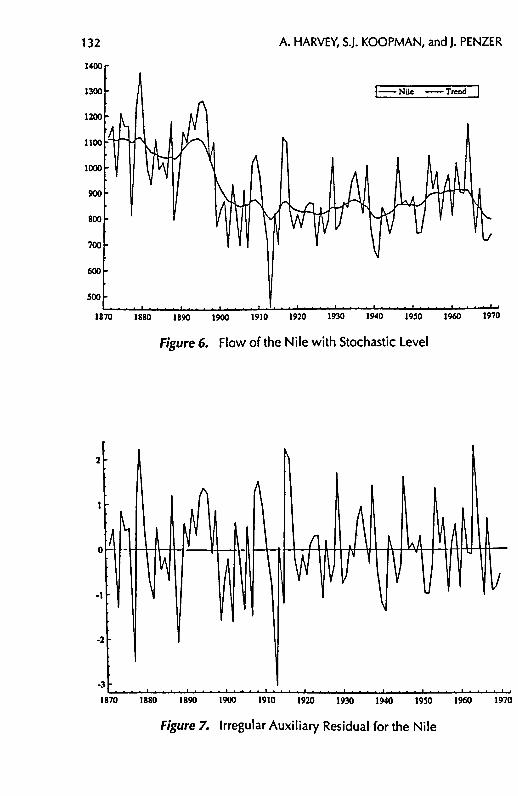
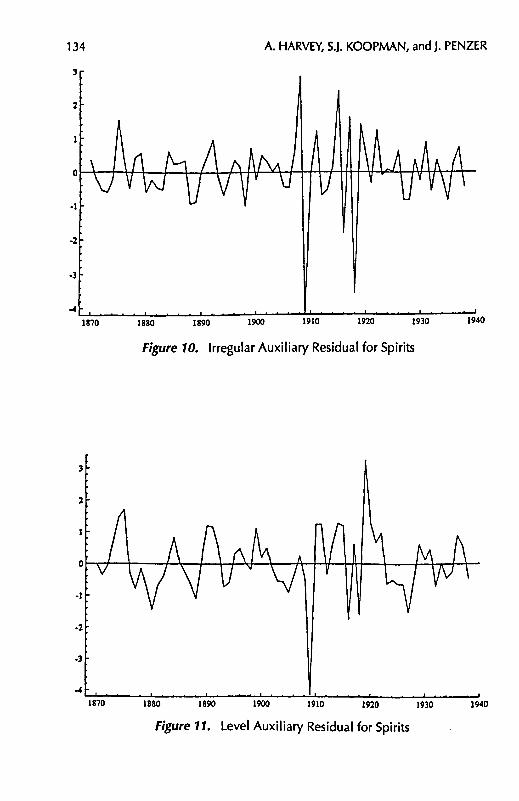
Example: The Flow of the Nile

Cobb (1978) gives a series of readings of the annual flow volume of the Nile River at Aswan for 1871 to 1970 (see Figure 6). This series has been analyzed more recently by Carlstein (1988) and Balke (1993). A random walk plus noise model, with oJ= 15099 and 0^ = 1469.2, fits the data well. The auxiliary residuals for the irregular and level components are plotted in Figures 7 and 8. Large irregular auxiliary residuals in 1877 and 1913 indicate outlying values. The level auxiliary residuals for the level suggest a level shift between 1897 and 1900, the most extreme value being in 1899. This corresponds with the construction of the first dam at Aswan which started in 1899 and was completely in 1902. Refitting the model with interventions for outliers in 1877 and 1913

A. HARVEY, S.J. KOOPMAN, and J. PENZER

1890 1900 1970

Figure 6. Flow of the Nile with Stochastic Level

1870 1880 1890 1900 1910 1920 1930 1940 19S0 1960

Figure 7. Irregular Auxiliary Residual for the Nile

1970

Messy Time Series

1870 1880 1890 1900 1910 1920 1930 1940 1950 1960 1970

Figure 8. Level Auxiliary Residual for the Nile

and a level shift in 1899, results in the variance of the stochastic level component becoming zero. Thus, once we have accounted for the structural break in 1899 there is no need for a stochastic level component (see Figure 9). This analysis is considerably more straightforward than the one put forward by Balke (1993). 1400 r

1870 1880 1890 1900 1910 1920 1930 1940 1950 1960 1970

Figure 9. Flow of the Nile with Deterministic Level Having Fitted Interventions

A. HARVEY, S.J. KOOPMAN, and J. PENZER

1870 1880 1890 1900 1910 1920 1930

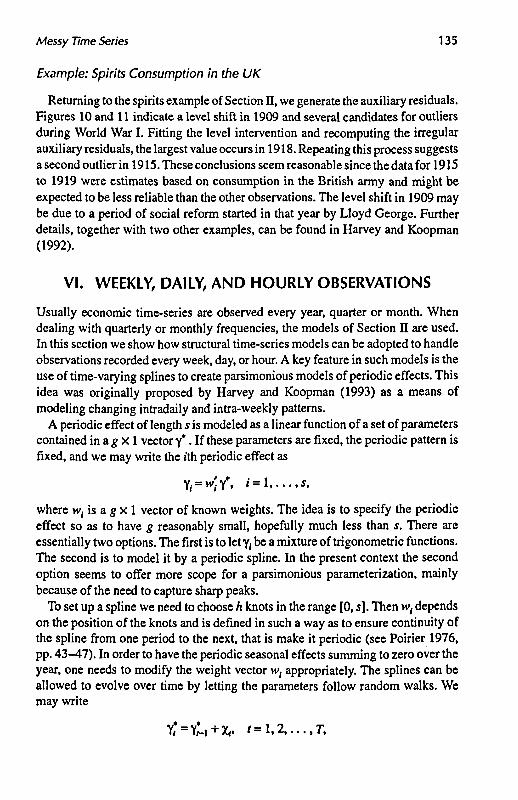
Figure 10. Irregular Auxiliary Residual for Spirits

1940

1870 1880 1890 1900 1910 1920 1930 1940

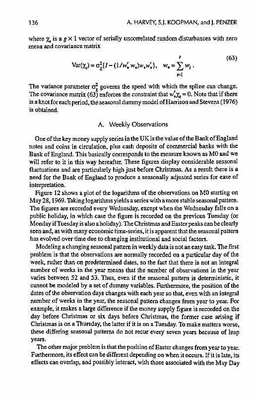
Figure 11. Level Auxiliary Residual for Spirits


Example: Spirits Consumption in the UK

Returning to the spirits example of Section II, we generate the auxiliary residuals. Figures 10 and 11 indicate a level shift in 1909 and several candidates for outliers during World War I. Fitting the level intervention and recomputing the irregular auxiliary residuals, the largest value occurs in 1918. Repeating this process suggests a second outlier in 1915. These conclusions seem reasonable since the data for 1915 to 1919 were estimates based on consumption in the British army and might be expected to be less reliable than the other observations. The level shift in 1909 may be due to a period of social reform started in that year by Lloyd George. Further details, together with two other examples, can be found in Harvey and Koopman (1992).

VI . WEEKLY, DAILY, AND HOURLY OBSERVATIONS

Usually economic time-series are observed every year, quarter or month. When dealing with quarterly or monthly frequencies, the models of Section II are used. In this section we show how structural time-series models can be adopted to handle observations recorded every week, day, or hour. A key feature in such models is the use of time-varying splines to create parsimonious models of periodic effects. This idea was originally proposed by Harvey and Koopman (1993) as a means of modeling changing intradaily and intra-weekly patterns.

A periodic effect of length s is modeled as a linear function of a set of parameters contained in a g X 1 vector y*. If these parameters are fixed, the periodic pattern is fixed, and we may write the ith periodic effect as

Y/^WJY*. * = 1 *•

where wi is a g x 1 vector of known weights. The idea is to specify the periodic effect so as to have g reasonably small, hopefully much less than s. There are essentially two options. The first is to let y,- be a mixture of trigonometric functions. The second is to model it by a periodic spline. In the present context the second option seems to offer more scope for a parsimonious parameterization, mainly because of the need to capture sharp peaks.

To set up a spline we need to choose h knots in the range [0, s]. Then w, depends on the position of the knots and is defined in such a way as to ensure continuity of the spline from one period to the next, that is make it periodic (see Poirier 1976, pp. 43-47). In order to have the periodic seasonal effects summing to zero over the year, one needs to modify the weight vector wt appropriately. The splines can be allowed to evolve over time by letting the parameters follow random walks. We may write

Y; = YM + X,, *=1,2 T,

136 A. HARVEY, SJ. KOOPMAN, and J. PENZER

where X, is a g x 1 vector of serially uncorrelated random disturbances with zero mean and covariance matrix

(63) Var(x,) = o*{/- (1/w, w > y . } . w. = £ w , .

i=l

The variance parameter a? governs the speed with which the spline can change. The covariance matrix (63) enforces the constraint that w'j^ = 0. Note that if there is a knot for each period, the seasonal dummy model of Harrison and Stevens (1976) is obtained.

A. Weekly Observations

One of the key money supply series in the UK is the value of the Bank of England notes and coins in circulation, plus cash deposits of commercial banks with the Bank of England. This basically corresponds to the measure known as MO and we will refer to it in this way hereafter. These figures display considerable seasonal fluctuations and are particularly high just before Christmas. As a result there is a need for the Bank of England to produce a seasonally adjusted series for ease of interpretation.

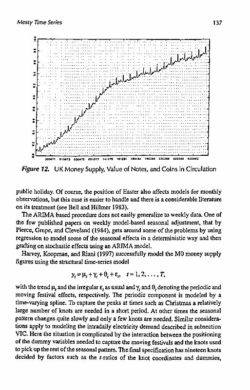
Figure 12 shows a plot of the logarithms of the observations on MO starting on May 28,1969. Taking logarithms yields a series with a more stable seasonal pattern. The figures are recorded every Wednesday, except when the Wednesday falls on a public holiday, in which case the figure is recorded on the previous Tuesday (or Monday if Tuesday is also a holiday). The Christmas and Easter peaks can be clearly seen and, as with many economic time-series, it is apparent that the seasonal pattern has evolved over time due to changing institutional and social factors.

Modeling a changing seasonal pattern in weekly data is not an easy task. The first problem is that the observations are normally recorded on a particular day of the week, rather than on predetermined dates, so the fact that there is not an integral number of weeks in the year means that the number of observations in the year varies between 52 and 53. Thus, even if the seasonal pattern is deterministic, it cannot be modeled by a set of dummy variables. Furthermore, the position of the dates of the observation days changes with each year so that, even with an integral number of weeks in the year, the seasonal pattern changes from year to year. For example, it makes a large difference if the money supply figure is recorded on the day before Christmas or six days before Christmas, the former case arising if Christmas is on a Thursday, the latter if it is on a Tuesday. To make matters worse, these differing seasonal patterns do not recur every seven years because of leap years.

The other major problem is that the position of Easter changes from year to year. Furthermore, its effect can be different depending on when it occurs. If it is late, its effects can overlap, and possibly interact, with those associated with the May Day


t • • • • • • • i • •

300671 01087} 03097) 0S1077 14117* K12S1 180184 1*0288 230368 0203*0 0306*2

Figure 12. UK Money Supply, Value of Notes, and Coins in Circulation

public holiday. Of course, the position of Easter also affects models for monthly observations, but this case is easier to handle and there is a considerable literature on its treatment (see Bell and Hillmer 1983).

The ARIMA based procedure does not easily generalize to weekly data. One of the few published papers on weekly model-based seasonal adjustment, that by Pierce, Grupe, and Cleveland (1984), gets around some of the problems by using regression to model some of the seasonal effects in a deterministic way and then grafting on stochastic effects using an ARIMA model.

Harvey, Koopman, and Riani (1997) successfully model the MO money supply figures using the structural time-series model

y,=n,+Y,+e,+e,. f=i*2 r, with the trend \it and the irregular e, as usual and yt and 0, denoting the periodic and moving festival effects, respectively. The periodic component is modeled by a time-varying spline. To capture the peaks at times such as Christmas a relatively large number of knots are needed in a short period. At other times the seasonal pattern changes quite slowly and only a few knots are needed. Similar considerations apply to modeling the intradaily electricity demand described in subsection VIC. Here the situation is complicated by the interaction between the positioning of the dummy variables needed to capture the moving festivals and the knots used to pick up the rest of the seasonal pattern. The final specification has nineteen knots decided by factors such as the /-ratios of the knot coordinates and dummies,


diagnostics and residual plots, goodness of fit statistics, and forecasting performance.

The effect of each public holiday is modeled by a set of dummy variables assigned to the surrounding weeks. The day of the year on which the holiday falls, and hence the days on which the surrounding observations fall, depends on the calendar. All moving public holidays in the UK fall on Mondays, except for Good Friday, and eleven stochastic dummy variables are specified to deal with them. No restrictions are put on these holiday effects, although this can easily be done. For example, the same state variable can be used for the spring and August Bank Holidays. An additional dummy is included in June 1977 to allow for the Queen's Silver Jubilee.

Another problem in weekly data is handling leap years. Harvey, Koopman, and Riani (1997) consider two different solutions. The first is to set the periodic effect for February 29 to be the same as those for February 28, that is, to regard day 59 as occurring twice. Proceeding in this way ensures that Christmas falls at exactly the same point every year, that is day 359. A slightly different approach is to let the leap year effect be spread throughout the whole year. In this case, the spline w( is modified by multiplying the knot positions by 366/365.

The residuals from the filtered model display considerable variability around Christmas. The impact of Christmas and the speed with which the pattern can change means a better model is found by doubling the variance of the Christmas knots. Doing this yields residuals much more akin to those in other parts of the year and reduces prediction errors.

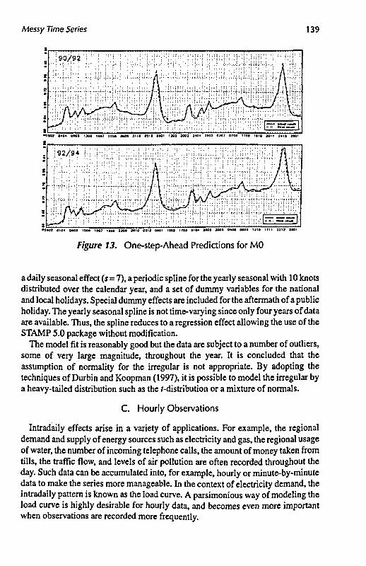
The validity of the model is illustrated by recent predictions. Figure 13 shows the one-step-ahead predictions obtained by filtering. It shows clearly the accuracy of the predictions; the prediction errors are less than 0.5 percent of the level most of the time.

B. Daily Observations

Structural time-series models can be extended to handle daily observations by introducing a daily component. This is modeled in the same way as a seasonal and can be allowed to evolve over time. Other components such as trend and annual seasonal pattern can be included as before.

The collection of papers in Bunn and Farmer (1985) gives an overview of the type of models which, until recently, have been employed in short-term forecasting of energy. The main approaches are based on ARIMA models, regression, exponential smoothing, or some mixtures of these. For daily observations the ARIMA airline model, based on the differencing operation AAj, is sometimes used. However, it is unlikely that one would identify such a model from the correlogram in the way Box and Jenkins (1976) advocate.

Gordon, Souza, and Koopman (1997) consider daily average consumption of electricity between January 1991 and December 1994 for three areas of Brazil (Minas Gerais, Rio de Janeiro, and Curitiba). The model includes a long-term trend,


» • - • . . . . : . •

•1001 0«0« M O >»* IH1 11M ]M> 1110 0111 OtOI 1X1 300) 2<0* JtO» 1X1 07M I lOt 1*10 1011 ]•<! 1HI

», ___~ _ . - ,

* ^ - , | • - 1 - I I - - - - "

•7MJ 0104 CMS 100* 1*07 I N I J JO* J«»0 03H SMI 1003 »*0J H0« 3*0* JO00 0«O« OMI UlO t?M 22 M 1W1

Figure 13. One-step-Ahead Predictions for MO

a daily seasonal effect (s=7), a periodic spline for the yearly seasonal with 10 knots distributed over the calendar year, and a set of dummy variables for the national and local holidays. Special dummy effects are included for the aftermath of a public holiday. The yearly seasonal spline is not time-varying since only four years of data are available. Thus, the spline reduces to a regression effect allowing the use of the STAMP 5.0 package without modification.

The model fit is reasonably good but the data are subject to a number of outliers, some of very large magnitude, throughout the year. It is concluded that the assumption of normality for the irregular is not appropriate. By adopting the techniques of Durbin and Koopman (1997), it is possible to model the irregular by a heavy-tailed distribution such as the /-distribution or a mixture of normals.

C. Hourly Observations

Intradaily effects arise in a variety of applications. For example, the regional demand and supply of energy sources such as electricity and gas, the regional usage of water, the number of incoming telephone calls, the amount of money taken from tills, the traffic flow, and levels of air pollution are often recorded throughout the day. Such data can be accumulated into, for example, hourly or minute-by-minute data to make the series more manageable. In the context of electricity demand, the intradaily pattern is known as the load curve. A parsimonious way of modeling the load curve is highly desirable for hourly data, and becomes even more important when observations are recorded more frequently.


Figure 14 shows the typical hourly pattern of electricity demand for a power company in the northwest of the United States in the summer and in the winter. The need for a time-varying periodic effect is apparent as the two patterns are clearly different. Also the average daily demand is much higher in winter.

The main purpose of the hourly model is to forecast future electricity demand two or three days ahead. The hourly model is given by

y, = u., + Y, + 5, + e,, f = l , 2 , . . . , r ,

with the trend \i{ and the irregular e, as usual and yt and 5, denoting the intradaily and explanatory effects, respectively. The irregular may also be modeled as a low order ARMA process to describe the remaining short-term dynamics in the series.

The standard intradaily effect is described by a periodic spline. A certain amount of experimentation is needed to determine the knot positions. To capture the peaks during the morning and the early evening periods, more knots are used at these times. Unfortunately, the same intradaily pattern will not apply to all days of the week; on Saturdays and Sundays the level of electricity demand and its intradaily pattern differs from that on weekdays. One way of handling this problem is to set up another spline which is zero at the begin and end of the day and which is added to the normal day spline. An alternative solution favored by Harvey and Koopman (1993) is to set up a spline for the whole week where the knots are restricted to have the same value for standard days.

3000

2500

2000

2000

1200

2000

1500

3 5 10 15 20 25

3500 "! Dec I

3000

2500

2000 L>w-e-^ 1 . . • • • - -

. * i _.

10 15 20 25

Figure 14. Typical Hourly Patterns of Electricity Demand


The introduction of explanatory variables into structural time-series models is straightforward; see subsection IIF. In the context of periodic time-series, explanatory variables may behave differently to the dependent variable yt at various stages of the seasonal cycle (winter/summer or morning/evening). When enough observations are available these different effects along the periodic pattern may be identified by setting up a periodic spline for the regression coefficient. The explanatory effect may be different for different values of the explanatory variable. For example, extreme temperature values have a pronounced effect on electricity demand (when it is cold, heating affects demand and when it is hot, air-conditioning affects demand) whereas moderate temperature values may not affect the electricity demand significantly. This nonlinear intra-temperature effect can be modeled by a cubic spline where the knot positions are placed within the range of temperature values.

VII. CONCLUSION

This review has covered a wide range of data irregularities and shown that the associated statistical problems can all be handled using a state space approach. Structural time-series models have intuitively appealing state space representations and the filter and smoother yield quantities which have practical interpretations. This gives structural models a clear advantage over ARIMA models when the data are messy. Furthermore, the specification of a suitable structural model is not dependent on an analysis of statistics, like the correlogram, which are subject to considerable distortion in the presence of data irregularities.

Structural models can be extended to deal with complicated time-varying periodic patterns. Recent research has also shown that the estimation of structural models with non-Gaussian disturbances is feasible using modern simulation methods. This has important implications for the fitting of models which are robust to outliers and structural change. The overall conclusion is that structural time-series models provide a unified and practical framework for dealing with messy time-series.

REFERENCES

Akaike, H. 1974. "Markovian Representation of Stochastic Processes and its Application to the Analysis of Autoregressive Moving Average Processes." Annals of the Institute of Statistical Mathematics 26: 363-387.

Anderson, B.D.O., and J.B. Moore. 1979. Optimal Filtering. Englewood Cliffs, NJ: Prentice-Hall. Ansley, C.F., and R. Kohn. 1985. "Estimation, Filtering and Smoothing in State Space Models with

Incompletely Specified Initial Conditions." Annals of Statistics 13(4): 1286-1316. Ansley, C.F., and R. Kohn. 1990. "Filtering and Smoothing in State Space Models with Partially Diffuse

Initial Conditions." Journal of Time Series Analysis 11(4): 275-294. Balke, N.S. 1993. "Detecting Level Shifts in Time Series." Journal of Business and Economic Statistics

11(1): 81-92.


Bell, W., and S. Hillmer. 1983. "Modeling Time Series with Calendar Variation." Journal of American Statistical Association 78:526-534.

Box, G.RR, and G.M. Jenkins. 1976. Time Series Analysis: Forecasting and Control. New York: Holden-Day, Inc.

Brubacher, S.R., and G. Tunnicliffe Wilson. 1976. "Interpolating Time Series with Application to the Estimation of Holiday Effects on Electricity Demand." Applied Statistics 25(2): 107-116.

Bruce, A.G., and R.D. Martin. 1989. "Leave-Jfc-out Diagnostics for Time Series." Journal of the Royal Statistical Society, Series B 51(3): 363-424.

Bunn, D., and E.D. Farmer. 1985. Comparitive Methods for Electrical Load Forecasting. New York: John Wiley and Sons.

Carlstein, E 1988. "Non-parametric Change Point Estimation." The Annals of Statistics 16:188-197. Chang, I., and G.C., Tiao, and C. Chen. 1988. "Estimation of Tune Series Parameters in Prescence of

Outliers." Technometrics 30(2): 193-204. Cobb, G.W. 1978. "The Problem of the Nile: Conditional Solution to a Change Point Problem."

Biometrika 65:243-251. De Jong, P. 1988. "A Cross-validation Filter for Time Series Models." Biometrika 75(3): 594-600. De Jong, P. 1989. "Smoothing and Interpolation with the State-space Model." Journal of the American

Statistical Association 84(408): 1085-1088. De Jong, P. 1991. "The Diffuse Kalman Filter." A nnals of Statistics 19(2): 1073-1083. De Jong, P., and J.R. Penzer. 1998. "Diagnosing Shocks in Time Series." Journal of the American

Statistical Association 93:796-806. Durbin, J., and S J. Koopman. 1997. "Monte Carlo Maximum Likelihood Estimation for Non-Gaussian

State Space Models." Biometrika 84:669-684. Fox, A.J. 1972. "Outliers in Time Series." Journal of the Royal Statistical Society Series B 34:350-363. Gordon, E, and R.C. Souza, and S.J. Koopman. 1997. "Forecasting Daily Electricity Demand Using

Splines." Mimeo. Harrison, P.J., and C.F. Stevens. 1976. "Bayesian Forecasting." Journal Royal Statistical Society Series

B 38:205-247. Harvey, A.C 1989. Forecasting, Structural Time Series Models and the Kalman Filter. New York:

Cambridge University Press. Harvey, A.C, and A. Jaeger. 1993. "Detrending Stylised Facts and the Business Cycle." Journal of

Applied Econometrics 8: 231-247. Harvey, A.C, and S J. Koopman. 1992. "Diagnostic Checking of Unobserved Component time Series

Models." Journal of Business and Economic Statistics 10(4): 377-389. Harvey, A.C, and S.J. Koopman. 1993. "Forecasting Hourly Electricity Demand Using Time-varying

Splines." Journal of the American Statistical Association 88:1228-1236. Harvey, A.C., S J. Koopman, and M. Riani. 1997. "The Modeling and Seasonal Adjustment of Weekly

Observations." Journal of Business and Economic Statistics 15:354-368. Harvey, A.C., and R.G. Pierse. 1984. "Estimating Missing Observations in Economic Time Series."

Journal of the American Statistical Association 79:125-131. Harvey, A.C, and A. Scott. 1994. "Seasonality in Dynamic Regression Models." Economic Journal

104:1324-1345. Harvey, A.C, and J.H. Stock. 1993. "Estimation, Smoothing, Interpolation and Distribution for

Structural Time-series Models in Continuous Time." Pp. 55-70 in Models, Methods and Applications of Econometrics, edited by P.C.B. Phillips. Oxford: Basil Blackwell.

Harvey, A.C, and M. Streibel. 1998. "Tests for Deterministic versus Indeterministic Cycles." Journal of Time Series Analysis 19: 505-530.

Harvey, A.C, and M. Streibel. 1997. "Testing Against Non-stationary Components." Mimeo. King, M.L., and G.H. Hillier. 1985. "Locally Best Invariant Tests of the Error Covariance Matrix in

Linear Regression Models." Journal of the Royal Statistical Society Series B 47:98-102.


Kohn, R., and C.F. Ansley. 1989. "A Fast Algorithm for Signal Extraction, Influence and Cross-validation in State Space Models." Biometrika 76(1): 65-79.

Koopman, S.J. 1993. "Disturbance Smoother for State Space Models." Biometrika 80(1): 117-126. Koopman, SJ. 1997. "Exact Initial Kalman Filter and Smoother for Non-stationary Time Series

Models." Journal of the American Statistical Association 92:1630-1638. Koopman, S J., A.C. Harvey, J.A. Doornik, and N. Shephard. 1995. STAMP 5.0: Structural Time Series

Analyser, Modeller and Predictor. London: Chapman and Hall. Koopman, S.J., and N. Shephard. 1992. "Exact Score for Time Series Models in State Space Form."

Biometrikal9(4): 823-826. LeFrancois, B. 1991. "Detecting Over-influential Observations in Time Series." Biometrika 78(1):

91-99. Lomnicki, Z.A. 1961. "Test for Departure from Normality in the Case of Linear Stochastic Processes."

Metrika 4:37-62. Maravall, A. 1985. "On Structural Time Series Models and the Characterization of Components."

Journal of Business and Economic Statistics 3:350-355. Muth, J.F. 1960. "Optimal Properties of Exponentially Weighted Forecasts." Journal of the American

Statistical Association 55: 299-305. Pearlman, J.G. 1980. "An Algorithm for the Exact Likelihood of a High-order Autoregressive-moving

Average Process." Biometrika 67(1): 232-233. Pierce, D.A., M.R. Grupe, and W.P. Cleveland. 1984. "Seasonal Adjustment of the Weekly Monetary

Aggregates: A Model-based Approach." Journal of Business and Economic Statistics 2:260-270. Poirier, D.J. 1976. The Econometrics of Structural Change, with special emphasis on Spline Functions.

Amsterdam: North Holland. Sargan, J.D., and E.G. Drettakis. 1974. "Missing Data in an Autoregressive Model." International

Economic Review 15:39-58. Snyder, R.D., and G.R. Saligari. 1996. "Initialization of the Kalman Filter with Partially Diffuse Initial

Conditions." Journal of Time Series Analysis 17(4): 409-424. Stock, J.H. 1994. "Unit Roots, Structural Breaks and Trends." Pp. 2740-2841 in Handbook of Econo

metrics, Volume 4, edited by R.F. Engle and D.L. McFadden. Amsterdam: Elsevier Science. Tsay, R.S. 1986. "Time Series Model Specification in the Presence of Outliers." Journal of the American

Statistical Association 81(393): 132-141. Tsay, R.S. 1988. "Outliers, Level Shifts and Variances Changes in Time Series." Journal of Forecasting

7:1-20. West, M., and PJ. Harrison. 1989. Bayesian Forecasting and Dynamic Models. New York: Springer

Verlag. Young, P. 1984. Recursive Estimation and Time Series Analysis. New York: Springer-Verlag.

MESSY TIME SERIES - stat.berkeley.edubrill/Stat248/messyts.pdf104 A. HARVEY S.J, . KOOPMAN, and J....

Documents

Transcript of MESSY TIME SERIES - stat.berkeley.edubrill/Stat248/messyts.pdf104 A. HARVEY S.J, . KOOPMAN, and J....