Message Passing Algorithms for Dirichlet

Diffusion Trees

David A. Knowles, University of CambridgeJurgen Van Gael, Microsoft Research CambridgeZoubin Ghahramani, University of Cambridge

May 6, 2011

Abstract

We demonstrate efficient approximate inference for the Dirichlet Dif-fusion Tree (Neal, 2003), a Bayesian nonparametric prior over tree struc-tures. Although DDTs provide a powerful and elegant approach for mod-eling hierarchies they haven’t seen much use to date. One problem is thecomputational cost of MCMC inference. We provide the first determin-istic approximate inference methods for DDT models and show excellentperformance compared to the MCMC alternative. We present messagepassing algorithms to approximate the Bayesian model evidence for aspecific tree. This is used to drive sequential tree building and greedysearch to find optimal tree structures, corresponding to hierarchical clus-terings of the data. We demonstrate appropriate observation models forcontinuous and binary data. The empirical performance of our methodis very close to the computationally expensive MCMC alternative on adensity estimation problem, and significantly outperforms kernel densityestimators.

1 Introduction

Tree structures play an important role in machine learning and statistics. Learn-ing a tree structure over data points gives a straightforward picture of howobjects of interest are related. Trees are easily interpreted and intuitive to un-derstand. Sometimes we may know that there is a true underlying hierarchy: forexample species in the tree of life or duplicates of genes in the human genome,known as paralogs. Typical mixture models, such as Dirichlet Process mixturemodels, have independent parameters for each component. In many situationswe might expect that certain clusters are similar, for example are sub-groups ofsome large group. By learning this hierarchical similarity structure, the modelcan share statistical strength between components to make better estimates ofparameters using less data.

1

In Bayesian modelling there is also a very good statistical reason to usetree structured prior distributions. By coupling priors through a tree structure,we allow posterior information to flow between the branches in the tree. Thissharing of statistical strength is often crucial for meaningful analysis in contextswhere little data is available.

Traditionally, a family of methods known as hierarchical clustering is used tolearn tree structures. Classical hierarchical clustering algorithms employ a bot-tom up “agglomerative” approach (Duda et al., 2001): start with a “hierarchy”of one datapoint and iteratively add the closest datapoint in some metric intothe hierarchy. The output of these algorithms is usually a binary tree or dendro-gram. Although these algorithms are straightforward to implement, both thead-hoc method and the distance metric hide the statistical assumptions beingmade.

Two solutions to this problem have recently been proposed. In Heller &Ghahramani the bottom-up agglomerative approach is kept but a principledprobabilistic model is used to find subtrees of the hierarchy. Bayesian evidenceis then used as the metric to decide which node to incorporate in the tree. Al-though fast, the lack of a generative process prohibits modeling uncertainty overtree structures. A different line of work (Williams, 2000; Neal, 2003; Teh et al.,2008; Blei et al., 2010; Roy et al., 2006) starts from a generative probabilisticmodel for both the tree structure and the data. Bayesian inference machinerycan then be used to compute posterior distributions on both the internal nodesof the tree as well as the tree structures themselves.

An advantage of the generative probabilistic models for trees is that theycan be used as a building block for other latent variable models (Rai & DaumeIII, 2008). We could use this technique to build topic models with hierarchieson the topics, or hidden Markov models where the states are hierarchicallyrelated. Greedy agglomerative approaches can only cluster latent variables afterinference has been done and hence they cannot be used in a principled way toaid inference in the latent variable model.

In this work we use the Dirichlet Diffusion Tree (DDT) introduced in Neal(2003), and reviewed in Section 2. This simple yet powerful generative modelspecifies a distribution on binary trees with multivariate Gaussian distributedvariables at the leaves. The DDT is a Bayesian nonparametric prior, and isa generalization of Dirichlet Process mixture models (Rasmussen, 2000). TheDDT can be thought of as providing a very flexible density model, since thehierarchical structure is able to effectively fit non-Gaussian distributions. In-deed, in Adams et al. (2008) the DDT was shown to significantly outperform aDirichlet Process mixture model in terms of predictive performance, and in factslightly outperformed the Gaussian Process Density Sampler. The DDT is thusboth a mathematically elegant nonparametric distribution over hierarchies andprovides state-of-the-art density estimation performance.

Our algorithms use the message passing framework (Kschischang et al., 2001;Minka, 2005). For many models message passing has been shown to significantlyoutperform sampling methods in terms of speed-accuracy trade-off. However,general α-divergence (Minka, 2005) based message passing is not guaranteed to

2

converge, which motivates our second, guaranteed convergent, algorithm whichuses message passing within EM (Kim & Ghahramani, 2006). Secondly, it isinherently parallelizable which is increasingly important on modern computerarchitectures. Thirdly, message passing algorithms are modular: the messagepassing rules for the DDT only need to be implemented once and can then easilybe combined with message passing on various latent variable model. Both algo-rithms are deterministic which confers various advantages over MCMC methods.Running inference on the same model and same data is reproducible. Conver-gence is simple compared to assessing convergence of a Markov chain.

The contributions of this paper are as follows. We derive and demonstratefull message passing (Section 3.1) and message passing within EM algorithms(Section 3.2) to approximate the model evidence for a specific tree, includingintegrating over hyperparameters (Section 3.3). We show how the resulting ap-proximate model evidence can be used to drive greedy search over tree structures(Section 3.4). We demonstrate that it is straightforward to connect differentobservation models to this module to model different data types, using binaryvectors as an example. Finally we present experiments using the DDT and ourapproximate inference scheme in Section 4.

2 The Dirichlet Diffusion Tree

The Dirichlet Diffusion Tree was introduced in Neal (2003) as a top-down gen-erative model for trees over N datapoints x1, x2, · · · , xN ∈ RD. The dataset isgenerated sequentially with each datapoint xi following the path of a Brownianmotion for unit time. We overload our notation by referring to the position ofeach datapoint at time t as xi(t) and define xi(1) = xi.

The first datapoint starts at time 0 at the origin in a D-dimensional Eu-clidean space and follows a Brownian motion with variance σ2 until time 1.If datapoint 1 is at position x1(t) at time t, the point will reach positionx1(t + dt) = x1(t) + Normal(0, σ2dt) at time t + dt. It can easily be shownthat x1(t) ∼ Normal(0, σ2t). The second point x2 in the dataset also startsat the origin and initially follows the path of x1. The path of x2 will divergefrom that of x1 at some time Td (controlled by the “divergence function” a(t))after which x2 follows a Brownian motion independent of x1(t) until t = 1. Inother words, the infinitesimal increments for the second path are equal to theinfinitesimal increments for the first path for all t < Td. After Td, the incrementsfor the second path Normal(0, σ2dt) are independent.

The generative process for datapoint i is as follows. Initially xi(t) follows thepath of the previous datapoints. If xi does not diverge before reaching a previousbranching point, the previous branches are chosen with probability proportionalto how many times each branch has been followed before. This reinforcementscheme is similar to the Chinese restaurant process (Aldous, 1985). If at timet the path for datapoint i has not yet diverged, it will diverge in the nextinfinitesimal time step dt with probability a(t)dt/m, where m is the number ofdatapoints that have previous followed the current path. The division by m is

3

0.0 0.2 0.4 0.6 0.8 1.0t

10

5

0

5

10

15

x

b

a

c

1

2

3

4

0

x1

x2

x3

x4

c

a

b

0

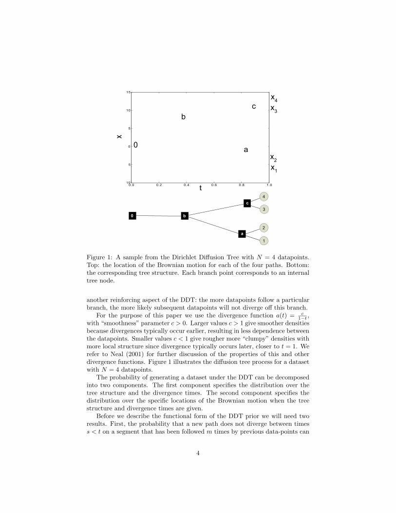
Figure 1: A sample from the Dirichlet Diffusion Tree with N = 4 datapoints.Top: the location of the Brownian motion for each of the four paths. Bottom:the corresponding tree structure. Each branch point corresponds to an internaltree node.

another reinforcing aspect of the DDT: the more datapoints follow a particularbranch, the more likely subsequent datapoints will not diverge off this branch.

For the purpose of this paper we use the divergence function a(t) = c1−t ,

with “smoothness” parameter c > 0. Larger values c > 1 give smoother densitiesbecause divergences typically occur earlier, resulting in less dependence betweenthe datapoints. Smaller values c < 1 give rougher more “clumpy” densities withmore local structure since divergence typically occurs later, closer to t = 1. Werefer to Neal (2001) for further discussion of the properties of this and otherdivergence functions. Figure 1 illustrates the diffusion tree process for a datasetwith N = 4 datapoints.

The probability of generating a dataset under the DDT can be decomposedinto two components. The first component specifies the distribution over thetree structure and the divergence times. The second component specifies thedistribution over the specific locations of the Brownian motion when the treestructure and divergence times are given.

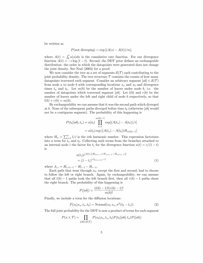
Before we describe the functional form of the DDT prior we will need tworesults. First, the probability that a new path does not diverge between timess < t on a segment that has been followed m times by previous data-points can

4

be written as

P (not diverging) = exp [(A(s)−A(t))/m],

where A(t) =∫ t0a(u)du is the cumulative rate function. For our divergence

function A(t) = −c log (1− t). Second, the DDT prior defines an exchangeabledistribution: the order in which the datapoints were generated does not changethe joint density. See Neal (2003) for a proof.

We now consider the tree as a set of segments S(T ) each contributing to thejoint probability density. The tree structure T contains the counts of how manydatapoints traversed each segment. Consider an arbitrary segment [ab] ∈ S(T )from node a to node b with corresponding locations xa and xb and divergencetimes ta and tb. Let m(b) be the number of leaves under node b, i.e. thenumber of datapoints which traversed segment [ab]. Let l(b) and r(b) be thenumber of leaves under the left and right child of node b respectively, so thatl(b) + r(b) = m(b).

By exchangeability we can assume that it was the second path which divergedat b. None of the subsequent paths diverged before time tb (otherwise [ab] wouldnot be a contiguous segment). The probability of this happening is

P (tb|[ab], ta) = a(tb)

m(b)−1∏i=1

exp[(A(ta)−A(tb))/i]

= a(tb) exp [(A(ta)−A(tb))Hm(b)−1]

where Hn =∑ni=1 1/i is the nth harmonic number. This expression factorizes

into a term for ta and tb. Collecting such terms from the branches attached toan internal node i the factor for ti for the divergence function a(t) = c/(1 − t)is

a(ti)e[A(ti)(Hl(i)−1+Hr(i)−1−Hm(i)−1)]

= (1− ti)cJl(i),r(i)−1 (1)

where Jl,r = Hr+l−1 −Hl−1 −Hr−1.Each path that went through xb, except the first and second, had to choose

to follow the left or right branch. Again, by exchangeability, we can assumethat all l(b) − 1 paths took the left branch first, then all r(b) − 1 paths chosethe right branch. The probability of this happening is

P ([ab]) =(l(b)− 1)!(r(b)− 1)!

m(b)!

Finally, we include a term for the diffusion locations:

P (xb|xa, ta, tb) = Normal(xb;xa, σ2(tb − ta)) (2)

The full joint probability for the DDT is now a product of terms for each segment

P (x, t, T ) =∏

[ab]∈S(T )

P (xb|xa, ta, tb)P (tb|[ab], ta)P ([ab])

5

3 Approximate Inference for the DDT

We assume that the likelihood can be written as a product of conditional prob-abilities for each of the leaves xn:

∏n l(yn|xn) where yn is observed data. Our

aim is to calculate the posterior distribution

P (x, t, T |y) =P (y, x, t, T )∑

T∫P (y, x, t, T )dxdt

Unfortunately, this integral is analytically intractable. Our solution is to usemessage passing or message passing within EM to approximate the marginallikelihood for a given tree structure: P (y|T ) =

∫P (y, x, t|T )dxdt. We use this

approximate marginal likelihood to drive tree building/search algorithm to finda weighted set of K-best trees.

3.1 Message passing algorithm

Here we describe our message passing algorithm for a fixed tree structure T .We employ the α-divergence framework from Minka (2005). Our variationalapproximation is fully factorized with a Gaussian q for every variable exceptc (the divergence function parameter) which is Gamma distributed. For eachsegment [ab] ∈ S(T ) we introduce two variables which are deterministic func-tions of existing variables: the branch length ∆[ab] = tb − ta and the variancev[ab] = σ2∆[ab]. We now write the unnormalized posterior as a product of fac-tors: ∏

n∈leaves

l(yn|xn)∏

[ab]∈S(T )

N(xb;xa, v[ab])

× δ(v[ab] − σ2∆[ab])δ(∆[ab] − (tb − ta))

× I(0 < ∆[ab] < 1)P (tb|T ) (3)

where δ(.) is the Dirac delta spike at 0, and I(.) is the indicator function. Thesefunctions are used to break down more complex factors into simpler ones forcomputational and mathematical convenience. Equation 3 defines a factor graphover the variables, shown in Figure 2.

Choosing α-divergences. We choose an α for each factor f in the factorgraph and then minimize the α-divergence Dα[q∼f (W )f(W )||q∼f (W )f(W )]with respect to f(W ) where W = x, t,∆, v is the set of latent variables for allnodes. Here

Dα(p||q) =1

α(1− α)

∫1− p(x)αq(x)(1−α)dx

is the α-divergence between two (normalized) distributions p and q; and q∼f (W ) =q(W )/f(W ) is the cavity distribution: the current variational posterior withoutthe contribution of factor f . Minka (2005) describes how this optimization canbe implemented as a message passing algorithm on the factor graph.

6

-N

N N --

P

0,1

×

-N

P

0,1

× -rN

0,1

×

1

0,1

P

N

I[0<x<1] constraint factorPrior factor on time (Eqn 1)Normal factor (Eqn 2)

α=1

α=1α=1α=0

α=1

Δ Δ

Δ

Figure 2: A subsection of the factor graph for the Dirichlet Diffusion Tree. Theleft node represents an internal node and is connected to two child nodes (notdepicted). The right node is a leaf node hence its location and divergence timeare observed (denoted in gray). The choice of α for the factors is shown forthe parent node. The hyperparameters σ2 and c which are connected to the ×(multiplication) factor and time prior P respectively are not shown.

We choose which α-divergence to minimize for each factor considering per-formance and computational tractability. The normal, minus, divergence timeprior and constraint factors use α = 1. The multiplication factor and prior ondivergence function parameter c use α = 0 (Figure 2). For the normal factorwe use α = 1 to attempt to approximate the evidence unbiasedly (α = 0 onlylower bounds the evidence, see Minka (2005)). The divergence time prior isnonconjugate so it is more straightforward to use α = 0 (EP). For the con-straint factors the divergence is infinite for α = 0 but analytic for α = 1. Forthe multiplication factor we use α = 0 due to the multimodal posterior (Sternet al., 2009). Since we only use α = 0 and 1 our algorithm can also be viewedas a hybrid Expectation Propagation (Minka, 2001) and Variational MessagePassing (Winn & Bishop, 2006)/mean field (Beal, 2003) algorithm. We use theInfer.NET (Minka et al., 2010) low level library of message updates to calculatethe outgoing message from each factor.

Further approximations. We found several approximations to the full mes-sage passing solution to be beneficial to the accuracy-speed trade-off of ouralgorithm.

• The message from the divergence time prior is a Beta distribution. Calcu-lating the true EP message when q(t) is Gaussian would require quadra-ture, which we found to be less accurate and more computationally ex-pensive than the following: map the incoming Gaussian message to aBeta distribution with the same mean and variance; multiply in the Beta

7

message; then map the outgoing message back to a Gaussian, again bymatching moments.

• For practically sized trees (i.e. with 10 or more leaves) we found themessage from the variance to the normal factor was typically quite peaked.We found no significant loss in performance in using only the mean ofthis message when updating the location marginals. In fact, since thisremoves the need to do any quadrature, we often found the performancewas improved.

• Similarly for the divergence function parameter c, we simply use the meanof the incoming message, since this was typically quite peaked.

Approximating the model evidence is required to drive the search over treestructures (see Section 3.4). Our evidence calculations follow Minka (2005), towhich we defer for details. We use the evidence calculated at each iteration toassess convergence.

Scheduling. Sensible scheduling of the message passing algorithm aided per-formance. The factor graph consists of two trees: one for the divergence lo-cations, one for the divergences times, with the branch lengths and variancesforming cross links between the trees. Belief propagation on a tree is exact: inone sweep up and then down the tree all the marginals are found. Althoughthis is not the case when the divergence times are unknown or KL projectionis required at the leaves, it implies that such sweeps will propagate informationefficiently throughout the tree, since EP is closely related to BP. To propagateinformation efficiently throughout this factor graph, our schedule consists of onesweep up and down the tree of locations and tree of times, followed by one sweepback and forth along the cross-links.

Usually one would start with the messages coming in from the prior: forexample for the divergence times. Unfortunately in our case these messagesare improper, and only result in proper marginals when the constraints thatta < tb are enforced through the constraint that the branch length ∆a→b mustbe positive. To alleviate this problem we initially set the message from the priorto spread the divergence times in the correct order, between 0 and 1, then runan iteration of message passing on the tree of divergence times, the constraints0 < ∆a→b < 1 and 0 < t < 1 and the prior. This results in proper variancemessages into the Normal factors when we sweep over the tree of location times.

3.2 Message passing in EM algorithm

For high dimensional problems we have found that our message passing algo-rithm over the divergence times can have convergence problems. This can beaddressed using damping, or by maximizing over the divergence times ratherthan trying to marginalize them. In high dimensional problems the divergencetimes tend to have more peaked posteriors because each dimension provides in-dependent information on when the divergence times should be. Because of this,

8

and because of the increasing evidence contribution from the increasing numberof Gaussian factors in the model at higher dimension D, modeling the uncer-tainty in the divergence times becomes less important. This suggests optimizingthe divergence times in an EM type algorithm.

In the E-step, we use message passing to integrate over the locations andhyperparameters. In the M-step we maximize the lower bound on the marginallikelihood with respect to the divergence times. While directly maximizing themarginal likelihood itself is in principle possible calculating the gradient withrespect to the divergence times is intractable since all the terms are all coupledthrough the tree of locations. For each node i with divergence time ti we havethe constraints tp < ti < min (tl, tr) where tl, tr, tp are the divergence times ofthe left child, right child and parent of i respectively.

One simple approach is to optimize each divergence time in turn (e.g. us-ing golden section search), performing a co-ordinate ascent. However, we foundjointly optimizing the divergence times using LBFGS (Liu & Nocedal, 1989) tobe more computationally efficient. Since the divergence times must lie within[0, 1] we use the reparameterization si = log [ti/(1− ti)] to extend the domainto the whole space, which we find improves empirical performance. From Equa-tions 2 and 1 the lower bound on the log evidence with respect to an individualdivergence time ti is

(〈c〉Jl(i),r(i) − 1) log (1− ti)− a log (ti − tp)− 〈1

σ2〉b[pi]

ti − tp

a =D

2, b[pi] =

1

2

D∑d=1

E[(xdi − xdp)2] (4)

where xdi is the location of node i in dimension d, and p is the parent ofnode i. The full lower bound is the sum of such terms over all nodes. Theexpectation required for b[pi] is readily calculated from the marginals of thelocations after message passing. Differentiating to obtain the gradient withrespect to ti is straightforward so we omit the details. The chain rule is usedto obtain the gradient with respect to the reparameterisation si, i.e. ∂·

∂si=

∂ti∂si

∂·∂ti

= ti(1 − ti)∂·∂ti

Although this is a constrained optimization problem(branch lengths cannot be negative) it is not necessary to use the log barriermethod because the 1/(ti − tp) terms in the objective implicitly enforce theconstraints.

3.3 Hyperparameter learning.

The DDT has two hyperparameters: the variance of the underlying Brownianmotion σ2 and the divergence function parameter c, which controls the smooth-ness of the data. For the full message passing framework, the overall variance σ2

is given a Gaussian prior and variational posterior and learnt using the multipli-cation factor with α = 0, corresponding to the mean field divergence measure.For the EM algorithm we use a Gamma prior and variational posterior for 1/σ2.

9

The message from each segment [ab] to 1/σ2 is then

m[ab]→1/σ2 = G

(D

2+ 1,

b[pi]

2(tb − ta)

)where G(α, β) is a Gamma distribution with shape α and rate β, and b[pi] is thesame as for Equation 4. The smoothness c is given a Gamma prior, and sentthe following VMP message from every internal node i:

〈log p(ti, c)〉 = log c+ (cJl(i),r(i) − 1)〈log(1− ti)〉⇒ mi→c = G

(c; 2,−Jl(i),r(i)〈log [1− ti]〉

)The term 〈log (1− ti)〉 is deterministic for the EM algorithm and is easily ap-proximated under the full message passing algorithm by mapping the Gaussianq(ti) to a Beta(ti;α, β) distribution with the same mean and variance, and not-ing that 〈log (1− ti)〉 = φ(β)− φ(α+ β) where φ(.) is the digamma function.

3.4 Search over tree structures

Our resulting message passing algorithm approximates the marginal likelihoodfor a fixed tree structure, p(y|T )p(T ) (we include the factor for the probabilityof the tree structure itself). Ideally we would now sum the marginal likelihoodover all possible tree structures T over N leaf nodes. Unfortunately, there are

(2N)!(N+1)!N ! such tree structures so that enumeration of all tree structures for even

a modest number of leaves is not feasible. Instead we maintain a list of K-besttrees (typically K = 10) which we find gives good empirical performance on adensity estimation problem.

We search the space of tree structures by detaching and re-attaching sub-trees, which may in fact be single leaves nodes. Central to the efficiency of ourmethod is keeping the messages (and divergence times) for both the main treeand detached subtree so that small changes to the structure only require a fewiterations of inference to reconverge.

We experimented with several heuristics for choosing which subtree to detachbut none significantly outperformed choosing a subtree at random. However, wegreatly improve upon attaching at random. We calculate the local contributionto the evidence that would be made by attaching the root of the subtree tothe midpoint of each possible branch. We then run inference on the L-bestattachments (L = 3 worked well, see Figure 5).

Sequential tree building. To build an initial tree structure we sequentiallyprocess the N leaves. We start with a single internal node with the first twoleaves as children. We run inference to convergence on this tree. Given a currenttree incorporating the first n − 1 leaves, we use the local evidence calculationdescribed above to propose L possible branches at which we could attach leafn. We run inference to convergence on the L resulting trees and choose the onewith the best evidence for the next iteration.

10

Tree search. Starting from a random tree or a tree built using the sequentialtree building algorithm, we can use tree search to improve the list of K-besttrees. We detach a subtree at random from the current best tree, and usethe local evidence calculation to propose L branches at which to re-attach thedetached subtree. We run message passing/EM to convergence in the resultingtrees, add these to the list of trees and keep only the K best trees in terms ofmodel evidence for the next iteration.

3.5 Predictive distribution

To calculate the predictive distribution for a specific tree we compute the dis-tribution for a new data point conditioned on the posterior location and diver-gence time marginals. Firstly, we calculate the probability of diverging fromeach branch according to the data generating process described in Section 2.Secondly we draw several (typically three) samples of when divergence fromeach branch occurs. Finally we calculate the Gaussian at the leaves resultingfrom Brownian motion starting at the sampled divergence time and location upto to t = 1. This results in a predictive distribution represented as a weightedmixture of Gaussians. Finally we average the density from the K-best treesfound by the algorithm.

3.6 Likelihood models

Connecting our DDT module to different likelihood models is straightforward.We demonstrate a Gaussian observation model for multivariate continuous dataand a probit model for binary vectors. Both factors use α = 1, correspondingto EP (Minka, 2001).

3.7 Computational cost

One iteration of message passing costs O(ND). Message passing therefore hascomplexity O(mND) where m is the number of iterations. m is kept small bymaintaining messages when changing the structure. The E-step of EM costsO(nND), where n is the number of iterations. With fixed σ and Gaussian ob-servations the E-step is simply belief propagation so n = 1. Usually n < mdue to not updating divergence times. The order k LBFGS in the M-step costsO(ksN), where s, the number of iterations, is typically small due to good ini-tialisation. So an iteration costs O(mND + skN). MCMC requires samplingthe divergence times using slice sampling: a single divergence time requires anO(ND) belief propagation sweep, giving total cost O(tN2D) where t is the num-ber of samples used before sampling the structure. The different scaling withN , combined with our more directed, greedy search confers our improvement inperformance.

11

4 Experiments

We tested our algorithms on both synthetic and real world data to assess com-putational and statistical performance both of variants of our algorithms andcompeting methods. Where computation times are given these were on a sys-tem running Windows 7 Professional with a Intel Core i7 2.67GHz quadcoreprocessor and 4GB RAM.

Toy 2D fractal dataset. Our first experiment is on a simple two dimensionaltoy example with clear hierarchical (fractal) structure shown in Figure 3, withN = 63 datapoints. Using the message passing in EM algorithm with sequentialtree building followed by 100 iterations of tree search we obtain the tree shown inFigure 3 in 7 seconds. The algorithm has recovered the underlying hierarchicalstructure of data apart from the occasional mistake close to the leaves where itis not clear what the optimal solution should be anyway.

0.8 0.6 0.4 0.2 0.0 0.2 0.4 0.6 0.81.5

1.0

0.5

0.0

0.5

1.0

1.5

Figure 3: Toy 2D fractal dataset(N=63) showing learnt tree structure.

2.0 1.5 1.0 0.5 0.0 0.5

1.5

1.0

0.5

0.0

0.5

1.0

Figure 4: First two dimensions of thesynthetic dataset from the prior withD = 5, N = 200, σ2 = 1, c = 1. Lighterbackground denotes higher probabilitydensity.

Data from the prior (D = 5, N = 200). We use a dataset sampled from theprior with σ2 = 1, c = 1, shown in Figure 4, to assess the different approachesto tree building and search discussing in Section 3.4. The results are shown inFigure 5. Eight repeats of each method were performed using different randomseeds. The slowest method starts with a random tree and tries randomly re-attaching subtrees (“search random”). Preferentially proposing re-attachingsubtrees at the best three positions significantly improves performance (“searchgreedy”). Sequential tree building is very fast (5-7 seconds), and can be followedby search where we only move leaves (“build+search leaves”) or better, subtrees

12

(“build+search subtrees”). The spread in initial log evidences for the sequentialtree build methods is due to different permutations of the data used for thesequential processing. This variation suggests tree building using several randompermutations of the data (potentially in parallel) and then choosing the bestresulting tree.

0 1 2 3 4 520

15

10

5

0

5

log

ev

ide

nce

/10

0

build+ search subt rees

build+ search leaves

search greedy

search random

time (min)

Figure 5: Performance of different tree building/search methods on the syntheticdataset.

Macaque skull measurements (N = 200, D = 10). We the macaque skullmeasurement data of Adams et al. (2008) to assess our algorithm’s performanceas a density model. Following Adams et al. (2008) we split the 10 dimensionaldata into 200 training points and 28 test points and model the three technicalrepeats separately. We compare to the infinite mixture of Gaussians (iMOGMCMC) and DDT MCMC methods implemented in Radford Neal’s FlexibleBayesian Modeling software (see http://www.cs.toronto.edu/∼radford/).As a baseline we use a kernel density estimate with bandwidth selected us-ing the npudens R package. The results are shown in Figure 6. The EM versionof our algorithm is able to find a good solution in just a few tens of seconds, butis eventually beaten on predictive performance by the MCMC solution. The fullmessage passing solution lies between the MCMC and EM solutions in termsof speed, and only outperforms the EM solution on the first of the three re-peats. The DDT based algorithms typically outperform the infinite mixture ofGaussians, with the exception of the second dataset.

Gene expression dataset (N = 2000, D = 171). We apply the EM algo-rithm with sequential tree building and 200 iterations of tree search to hierarchi-cal clustering of the 2000 most variable genes from Yu & Landsittel (2004). Wecalculate predictive log likelihoods on four splits into 1800 training and 200 test

13

per

inst

ance

impr

ovem

ent

over

kde

(na

ts)

time (min) time (min) time (min)

Figure 6: Per instance test set performance on the macaque skull measurementdata Adams et al. (2008). The three plots arise from using the three technicalreplicates as separate datasets.

iMOG DDT EM DDT MCMCScore −1.00± 0.04 −0.91± 0.02 −0.88± 0.03Time 37min 48min 18hours

Table 1: Results on a gene expression dataset (Yu & Landsittel, 2004). Score isthe per test point, per dimension log predictive likelihood. Time is the averagecomputation time on the system described in Section 4.

genes. The results are shown in Table 1. The EM algorithm for the DDT hascomparable statistical performance to the MCMC solution whilst being an or-der of magnitude faster. Both implementations significantly outperform iMOGin terms of predictive performance. DDT MCMC was run for 100 iterations,where one iteration involves sampling the position of every subtree, and thescore computed averaging over the last 50 samples. Running DDT MCMC for5 iterations takes 54min (comparable to the time for EM) and gives a score of−0.98± 0.04, worse than DDT EM.

Animal species. To demonstrate the use of an alternative observation modelwe use a probit observation model in each dimension to model 102-dimensionalbinary feature vectors relating to attributes (e.g. being warm-blooded, havingtwo legs) of 33 animal species (Kemp & Tenenbaum, 2008). The tree struc-ture we find, shown in Figure 7, is intuitive, with subtrees corresponding toland mammals, aquatic mammals, reptiles, birds, and insects (shown by colourcoding).

5 Related work

We briefly discuss some relevant related work.Kingman’s coalescent (Teh et al., 2008) is similar to the Dirichlet Diffusion

Tree in spirit although the generative process is defined going backwards in time

14

as datapoints coalesce together, rather than forward in time as for the DDT.Efficient inference for Kingman’s coalescent was demonstrated in Teh & Gorur(2009). We leave investigating whether our framework could be adapted to thecoalescent as future work.

In Bayesian Hierarchical Clustering (Heller & Ghahramani) the bottom-upagglomerative approach is kept but a principled probabilistic model is used tofind subtrees of the hierarchy. Bayesian evidence is then used as the metric todecide which node to incorporate in the tree. The model works for continuousdata but the R package only supports categorical data, whereas our quantitativeassessments use continuous data. On the “Animals” example the tree obtainedis broadly consistent. BHC is faster than our method, taking 3s vs 30s for DDTEM (the difference would be less for continuous data where we do not requireEP). However, BHC is not a generative model and so cannot be coherentlyincorporated into larger models.

Roy et al. (2006) present an elegant model, but one which is only directlyapplicable to binary data: a sensible extension to continuous data is not obvious.

In the model of Williams (2000) each child chooses a parent in the layerabove. The number of layers and nodes per layer must be pre-specified: learningthis in fact gave worse results. Unlike the DDT, the model is parametric, so itscomplexity cannot adapt to the data.

The nested CRP Blei et al. (2010) is an alternative generative model whichdefines probability distributions over tree structures. One difference to the DDTthough is that it does not share the property that two nodes close in the treeare correlated: rather, it models each data point as a mixture over the nodeson the path from the root to that data point. A variational inference procedurefor the nCRP has recently been introduced by Wang & Blei.

6 Conclusion

Our approximate inference scheme, combining message passing and greedy treesearch, is a computationally attractive alternative to MCMC for DDT mod-els. We have demonstrated the strength of our method for modeling observedcontinuous and binary data at the leaves, and hope that by making code avail-able we will encourage the community to use this elegant prior over hierarchies.In ongoing work we use the DDT to learn hierarchical structure over latentvariables in models including Hidden Markov Models, specifically in part ofspeech tagging (Kupiec, 1992) where a hierarchy over the latent states aids in-terpretability, and Latent Dirichlet Allocation, where it is intuitive that topicsmight be hierarchically clustered (Blei et al., 2004).

References

Adams, Ryan, Murray, Iain, and MacKay, David. The Gaussian process densitysampler. In Advances in Neural Information Processing Systems, volume 21.

15

MIT Press, 2008.

Aldous, D. Exchangeability and related topics. In Ecole d’Ete de Probabilitiesde Saint-Flour, volume XIII, pp. 1–198, 1985.

Beal, M. J. Variational algorithms for approximate Bayesian inference. PhDthesis, Gatsby Computational Neuroscience Unit, University College London,2003.

Blei, D. M., Griffiths, T. L., Jordan, M. I., and Tenenbaum, J. B. Hierarchicaltopic models and the nested Chinese restaurant process. Advances in NeuralInformation Processing Systems, 16:106, 2004.

Blei, David M., Griffiths, Thomas L., and Jordan, Michael I. The nested chineserestaurant process and Bayesian nonparametric inference of topic hierarchies.Journal of the ACM, 57, 2010.

Duda, R. O., Hart, P. E., and Stork, D. G. Pattern Classification. Wiley-Interscience, 2nd edition, 2001.

Heller, K. A. and Ghahramani, Z. In Proceedings of the 22nd InternationalConference on Machine learning, pp. 304.

Kemp, Charles and Tenenbaum, Joshua B. The discovery of structural form. InProceedings of the National Academy of Sciences, volume 105(31), pp. 10687–10692, 2008.

Kim, H.-C. and Ghahramani, Z. Bayesian Gaussian process classification withthe EM-EP algorithm. In IEEE Transactions on Pattern Analysis and Ma-chine Intelligence, volume 28, pp. 1948–1959, 2006.

Kschischang, F. R., Frey, B. J., and Loeliger, H. A. Factor graphs and the sum-product algorithm. IEEE Transactions on information theory, 47(2):498519,2001.

Kupiec, Julian. Robust part-of-speech tagging using a hidden markov model.Computer Speech & Language, 6(3):225 – 242, 1992. ISSN 0885-2308.

Liu, D. C. and Nocedal, J. On the limited memory bfgs method for large scaleoptimization. Math. Program., 45:503–528, December 1989. ISSN 0025-5610.

Minka, T. P. Expectation propagation for approximate bayesian inference. InUncertainty in Artificial Intelligence, 2001.

Minka, T. P. Divergence measures and message passing. Microsoft Research,Cambridge, UK, Tech. Rep. MSR-TR-2005-173, 2005.

Minka, T. P., Winn, J. M., Guiver, J. P., and Knowles, D. A. Infer.NET 2.4,2010. Microsoft Research Cambridge. http://research.microsoft.com/infernet.

16

Neal, R. M. Defining priors for distributions using Dirichlet diffusion trees.Technical Report 0104, Dept. of Statistics, University of Toronto, 2001.

Neal, R. M. Density modeling and clustering using Dirichlet diffusion trees.Bayesian Statistics, 7:619–629, 2003.

Rai, Piyush and Daume III, Hal. The infinite hierarchical factor regressionmodel. In Advances in Neural Information Processing Systems, volume 21.MIT Press, 2008.

Rasmussen, C. E. The infinite Gaussian mixture model. Advances in NeuralInformation Processing Systems, 12:554–560, 2000.

Roy, Daniel M., Kemp, Charles, Mansinghka, Vikash K., and Tenenbaum,Joshua B. Learning annotated hierarchies from relational data. In Advancesin Neural Information Processing Systems, volume 19, 2006.

Stern, D.H., Herbrich, R., and Graepel, T. Matchbox: large scale online bayesianrecommendations. In Proceedings of the 18th international conference onWorld wide web, pp. 111120. ACM New York, NY, USA, 2009. URL http:

//portal.acm.org/citation.cfm?id=1526709.1526725.

Teh, Y. W., Daume III, H., and Roy, D. M. Bayesian agglomerative clusteringwith coalescents. Advances in Neural Information Processing Systems, 20,2008.

Teh, Y.W. and Gorur, D. An Efficient Sequential Monte Carlo Algorithm forCoalescent Clustering. Advances in Neural Information Processing Systems,2009.

Wang, C. and Blei, D.M. Variational Inference for the Nested Chinese Restau-rant Process. cs.princeton.edu, pp. 1–9. URL http://www.cs.princeton.

edu/~blei/papers/WangBlei2009d.pdf.

Williams, C. A MCMC approach to hierarchical mixture modelling. Advancesin Neural Information Processing Systems, 13, 2000.

Winn, J. and Bishop, C. M. Variational message passing. Journal of MachineLearning Research, 6(1):661, 2006.

Yu, Y. P. and Landsittel, D. et al. Gene expression alterations in prostatecancer predicting tumor aggression and preceding development of malignancy.Journal of Clinical Oncology, 22(14):2790–2799, Jul 2004.

17

Ant

Bee

Cockroach

Butterfly

Trout

Salmon

Seal

Whale

Dolphin

Penguin

Ostrich

Chicken

Finch

Robin

Eagle

Iguana

Alligator

Tiger

Lion

Cat

Wolf

Dog

Squirrel

Mouse

Gorilla

Chimp

Deer

Cow

Elephant

Camel

Giraffe

Rhino

Horse

Figure 7: Tree structure learnt over animals using 102 binary features with theprobit observation model.

18