1

Merging-based forward-backward smoothing onGaussian mixtures

Abu Sajana Rahmathullah ∗, Lennart Svensson∗, Daniel Svensson†∗Department of Signals and Systems, Chalmers University of Technology, Sweden

†Electronic Defence Systems, SAAB AB, SwedenEmails: {sajana, lennart.svensson, daniel.svensson}@chalmers.se

Abstract—Conventional forward-backward smoothing (FBS)for Gaussian mixture (GM) problems are based on pruningmethods which yield a degenerate hypothesis tree and often leadto underestimated uncertainties. To overcome these shortcomings,we propose an algorithm that is based on merging componentsin the GM during filtering and smoothing. Compared to FBSbased on the N−scan pruning, the proposed algorithm offersbetter performance in terms of track loss, root mean squarederror (RMSE) and normalized estimation error squared (NEES)without increasing the computational complexity.

Index Terms—filtering, smoothing, Gaussian mixtures,forward-backward smoothing, data association

I. INTRODUCTION

Gaussian mixture (GM) densities appear naturally in a rangeof different problems. One such problem is target tracking inthe presence of clutter, which is a challenging problem in manysituations. Under linear and Gaussian assumptions for themotion and sensor models, there exists a closed form optimalsolution for this problem. The optimal solution for filteringand smoothing involves GMs, with an exponentially increasingnumber of components as a function of the product of thenumber of measurements across time. Thus, approximationsare inevitable to reduce the complexity.

The optimal solution to GM filtering retains several trackhypotheses for the target, along with a probability or weightfor each hypothesis. In target tracking, each track hypothesishas a sequence of data association (DA) hypotheses associatedto it, and corresponds to a component in the GM. Thesequence of DAs across time is usually illustrated using agraphical structure, the hypothesis tree. Along each branch inthe hypothesis tree, there is a sequence of Gaussian densitiesacross time, along with the probability for the correspondinghypothesis sequence. Within the family of multiple hypothesistracking (MHT) algorithms [1, 10], a large quantity employpruning as a means to reduce the number of branches inthe tree (or components in the GM) at each time. As aresult, the uncertainty about the DA hypotheses is significantlyunderestimated if the pruning is aggressive. If the track withthe correct DAs was pruned during the pruning step, it can alsolead to incorrect DAs (being retained after pruning) during thesubsequent time instants, eventually leading to track loss.

In fixed-interval smoothing, the goal is to estimate a se-quence of state variables given the data observed at all times,i.e., given a batch of data. There are two main approaches to

smoothing: forward-backward smoothing (FBS) [9] and two-filter smoothing [6]. In theory, these two methods are optimaland thus identical, but in practice they often differ due toapproximations made in order to obtain practical implemen-tations. In GM smoothing, we are normally forced to useapproximations during both the filtering and smoothing steps.Therefore, the performance depends on the approximationsmade during both the filtering and smoothing steps.

In the conventional FBS implementations [4, 6, 8], theforward filtering (FF) method is performed using a traditionalpruning-based filtering algorithm, such as an MHT. For thebackward smoothing (BS) step, Rauch-Tung-Striebel (RTS)smoothing is used along each branch in the hypothesis treeto obtain the smoothing posterior. Along with the Gaussiandensities, the weights of all branches are also computed. Theobtained solution is optimal, if there is no pruning (or merging)employed during FF. If the FF algorithm is based on pruning,we usually perform BS on a degenerated hypothesis tree. Thatis, the tree usually indicates that there is a large number of DAhypotheses at the most recent times, but only one hypothesisat earlier times. Degeneracy is not necessarily an issue for thefiltering performance as that mainly depends on the descriptionof the most recent DA hypotheses. However, during BS wealso make extensive use of the history of DA hypotheses,which is often poorly described by a degenerate hypothesistree. There is always a risk that a correct hypothesis is prunedat least at some time instances. BS on this degenerate tree isnot going to help in improving the accuracy of the DA. Attimes when the degenerate tree contains incorrect DAs, themean of the smoothing posterior may be far from the correctvalue. Even worse, since the smoother is unaware of the DAuncertainties, it will still report a small posterior covariancematrix indicating that there are little uncertainties in the state.

The degeneracy of the hypothesis tree in GM forwardfiltering is closely related to the well known degeneracy ofthe number of surviving particles in a particle filter. There hasbeen a lot of work done in the existing literature regardingdegeneracy in particle filter smoothing ([3, 5, 7]). Most ofthese discuss the degeneracy issue extensively. However, theideas proposed in the particle smoothing literature have not yetled to any improvements in the treatment of the degeneracyin the GM smoothing context.

In this paper, we propose merging during FF as a wayto avoid the occurrence of degenerate trees. We consider theproblem of tracking a single target in a clutter background, in

which case the posterior densities are GMs. We present a strat-egy for FF and BS on GMs that involves merging and pruningapproximations which we refer to as FBS-GMM (stands forforward-backward smoothing with Gaussian mixture merging).Once merging is introduced, we get a hypothesis graph insteadof a hypothesis tree. Using the graphical structure, we discussin detail how BS can be performed on the GMs that areobtained as a result of merging (and pruning) during FF.

The FBS-GMM is compared to an FBS algorithm thatuses N−scan pruning during FF. The performance measurescompared are root mean squared error (RMSE), track loss,computational complexity and normalized estimation errorsquared (NEES). When it comes to track loss, NEES and com-plexity, the merging based algorithm performs significantlybetter than the pruning based one for comparable RMSE.

II. PROBLEM FORMULATION AND IDEA

We consider a single target moving in a clutter background.The state vector xk is varying according to the process model,

xk = Fxk−1 + vk, (1)

where vk ∼ N (0, Q). The target is detected with probabilityPD. The target measurement, when detected, is given by

ztk = Hxk + wk (2)

where wk ∼ N (0, R). The measurement set Zk is theunion of the target measurement (when detected) and a set ofclutter detections. The clutter measurements are assumed tobe uniformly distributed in the observation region of volumeV . The number of clutter measurements is Poisson distributedwith parameter βV , where β is the clutter density. The numberof measurements obtained at time k is denoted mk.

The objective is to find the smoothing density p(xk|Z1:K)for k = 1, ...,K using FBS, and to compare different imple-mentation strategies. If pruning is the only method used formixture reduction during FF, it is straightforward to use RTSiterations to perform BS. However, if the FF approximationsinvolve merging as well, then we need to show how the RTSiterations can be used for the merged components.

A. Idea

The shortcoming of performing BS after pruning-based FFis that the DA uncertainties are typically completely ignoredfor the early parts (often the majority) of the time sequence,due to pruning in the FF. This can be easily illustrated using agraphical structure, called an hypothesis tree. The hypothesistree captures different DA sequences across time. The nodesin the graph correspond to the components of the filtering GMdensity. Naturally, a pruned node will not have any offsprings.Let us consider the example in Fig. 1. To the left, the figureshows the tree during FF using N−scan pruning (with N = 2).To the right in the figure is the resulting degenerate tree afterFF is completed. This example can be extended to generalizethat, for k � K, the tree after pruning-based FF will bedegenerate. By performing BS on the degenerate tree, the DAuncertainties can be underestimated greatly.

Fig. 1: Example of a degenerate tree after FF with N−scan pruningwith N = 2. To the left, the figure shows the tree with the nodes that arepruned. In the figure to the right, the pruned branches are removed. Onecan see that eventually only one branch is retained from time 1 to 4.

Fig. 2: Same example as in Fig. 1. Here, instead of pruning, merging ofcomponents is performed. One can see that the DA uncertainties are stillretained in the merged nodes.

To overcome this weakness, one can perform merging of thenodes in the hypothesis tree instead of pruning. One can alsoillustrate the merging procedure during FF using a hypothesisgraph, herein called the f-graph (not a tree in this case).Consider the same example shown in Fig. 2, with merginginstead of pruning. To the left, one can see the graph withmerging performed at several places and to the right, theresult after FF that uses merging. It is clear that there is nodegeneracy after merging-based FF. The idea in this paper isto develop a BS algorithm on the graph obtained after FFwith merging. The smoothing density is also a GM, whereGM reduction (GMR) can be employed. We use graphicalstructures to illustrate the FF and BS and define hypothesescorresponding to each node in the graphs to calculate theweights of different branches.

III. BACKGROUND

In this section, we discuss the optimal FBS of GMs and howFBS can be performed with approximations based on pruningstrategies. Towards the end of the section, FF using mergingapproximations is also discussed. The graphical structures inall of these scenarios are explained. In the next section, itwill be shown how a similar graph structure can be created toillustrate the BS in a merging-based filter.

A. Forward-Backward Smoothing

In smoothing, we are interested in finding the smoothingposterior, p(xk|Z1:K). This density can be written as,

p(xk|Z1:K) ∝ p(xk|Z1:k)p(Zk+1:K |xk). (3)

Fig. 3: Optimal Gaussian mixture filtering and smoothing are illustratedin a hypothesis tree. At each time, each node represents a componentin the filtering GM at the corresponding time. The solid arrowed linesrepresent the data associations across time. The dashed arrowed linesrepresent the paths taken while performing backward smoothing fromeach leaf node back to the nodes at time K− 1. During BS, these pathscontinue until the root node.

In (3), the smoothing posterior is obtained by updating the fil-tering posterior p(xk|Z1:k) with the likelihood p(Zk+1:K |xk).This update step is analogous to the update step in theKalman filter. The filtering density p(xk|Z1:k) is obtainedusing a forward filter. In the FBS formulation, the likelihoodis obtained from the filtering density recursively as

p(Zk+1:K |xk) ∝ˆp(Zk+1:K |xk+1) f(xk+1|xk) dxk+1,

(4)

wherep(Zk+1:K |xk+1) ∝

p(xk+1|Z1:K)

p(xk+1|Z1:k). (5)

A problem with (5) is that it involves division of densities.In the simple case, when the two densities p(xk+1|Z1:k) andp(xk+1|Z1:K) are Gaussian, the division is straightforward.Then, the RTS smoother [9] gives a closed-form expressionfor the likelihood in (5) and the smoothing posterior in (3).But, for GM densities, this division does not have a closed-form solution, in general.

B. Optimal Gaussian mixture FBS

In a target-tracking problem with clutter and/or PD < 1, itcan be shown that the true filtering and smoothing posteriordensities at any time k are GMs [8]. The filtering density GMis

p(xk|Z1:k) =

Mfk∑

n=0

p(xk|Z1:k,Hfk,n)Pr

{Hf

k,n|Z1:k

},(6)

where Mfk is the number of components in the GM (for

the optimal case, Mfk =

k∏i=1

(mi + 1)). The hypothesis Hnk

represents a unique sequence of measurements or missed-detection hypotheses assignments from time 1 to time k, underwhich the density p(xk|Z1:k,Hf

k,n) is obtained. The missed-detection assignment can also be viewed as a measurementassignment and will be treated so in the rest of this paper.

The FF procedure in the optimal case is illustrated in thehypothesis tree in Fig. 3. Each node n at time k in the

tree represents a Gaussian density p(xk|Z1;k,Hfk,n) and a

probability Pr{Hf

k,n|Z1:k

}.

As was pointed out in Section III-A, BS involves division ofdensities. Since the densities involved here are GMs, we wantto avoid the division of densities as it is difficult to handlein most situations. To overcome this difficulty, the smoothingdensity p(xk|Z1:K) is represented as

p(xk|Z1:K) =

MfK∑

a=0

p(xk|Z1:K ,HfK,a)Pr

{Hf

K,a|Z1:K

}, (7)

where each component p(xk|Z1:K ,HfK,a) is obtained by per-

forming RTS using the filtering densities along every branchof the hypothesis tree (cf. Fig. 3).

C. Forward filter based on pruning and merging approxima-tions

In this section, we discuss the different existing suboptimalstrategies that are used in performing FF when the posteriordensities are GMs. These methods are based on merging andpruning the branches in the hypothesis tree.

1) Pruning-based filter: In pruning, the nodes that havelow values for Pr

{Hf

K,a|Z1:K

}are removed. The way the

low values are identified can vary across different pruningstrategies. One advantage of pruning is that it is simple to im-plement, even in multiple targets scenarios. A few commonlyused pruning strategies are threshold-based pruning, M -bestpruning and N -scan pruning [1].

The disadvantage of any pruning scheme is that in complexscenarios, it can happen that we have too many componentswith significant weights, but we are forced to prune someof them to limit the number of components for complexityreasons. For instance, if many components correspondingto the validated measurements have approximately the sameweights, then it may not be desirable to prune some of thecomponents. However, the algorithm might prune the compo-nents that correspond to the correct hypothesis, leading to trackloss. One other drawback of pruning is that the covarianceof the estimated state can be underestimated because thecovariances of the pruned components are lost. This can leadto an inconsistent estimator, with a bad NEES performance.Also, as was shown in Fig. 1, pruning during FF often returnsdegenerate trees.

BS on trees obtained after pruning-based FF is performedin a similar way as in the optimal case discussed in SectionIII-B. However, the number of branches in this tree is lesser,because of which the number of RTS smoothers run is alsoless. The readers are referred to [10] and [1] for more detailsof FBS on GM with pruning-based approximations.

2) Merging-based filter: To overcome the degeneracy prob-lem in pruning-based FF, one can use a merging (or acombination of merging and pruning) algorithm to reduce thenumber of components in the filtering density, instead of onlypruning the components. In merging, the components whichare similar are approximated as identical and replaced withone Gaussian component that has the same first two moments.Merging can be represented in the hypothesis tree with several

Fig. 4: A part of an f-graph is shown to illustrate merging during forwardfiltering (FF) (solid lines) and backward smoothing (BS) through mergednodes (dashed lines). The solid lines represent the branches in the FF.The small filled circles represent the components before merging. Thedashed lines illustrate that each incident component on the merged nodei while smoothing can split into many components. The hypothesis andthe parameters in the box are discussed in Section IV-A1.

components being incident on the same node as shown in Fig.4. Therefore, the structure of the hypothesis tree changes froma tree to a generic graph, which we refer as the f-graph.

There are several merging strategies discussed in [12], [11]and [2], which are used for GMR. Two main criteria for choos-ing the appropriate GMR algorithm are the computationalcomplexity involved and the accuracy. Merging strategies willbe discussed briefly in Section VI-B.

As a tradeoff between complexity and track loss perfor-mance, it is more feasible to use pruning along with merging,since pruning can be performed quickly. Pruning ensures thatthe components with negligible weights are removed, withoutbeing aggressive. Merging reduces the number of componentsfurther. This combination of pruning and merging ensures thatthe computations are under control without compromising toomuch on the performance.

IV. BACKWARD SMOOTHING THROUGH MERGED NODES

In the previous section, it was discussed how optimalGM filtering and smoothing can be performed. It was alsodiscussed how approximations such as merging and pruningare employed during FF. We also observed that FBS issimple to apply when the FF algorithm uses pruning but notmerging. In this section, we discuss in detail how BS can beperformed after an FF step that involves pruning and mergingapproximations.

The idea behind BS on a hypothesis graph with mergednodes can be understood by first analyzing how BS works ona hypothesis tree obtained after pruning-based forward filter.As mentioned in Section III-B, in the pruning-based FF, eachcomponent in the filtering density p(xk|Z1:k) corresponds toa hypothesis Hf

k,n, which is a unique DA sequence from time1 to time k. BS is then performed to obtain the smoothingdensity as described in (7). Each component in (7) is obtainedby using an RTS smoother, which combines a componentp(xk+1|Z1:K ,Hf

K,a) in the smoothing density at time k + 1

and a component p(xk|Z1:k,Hfk,n) in the filtering density at k,

such that p(xk|Z1:k,Hfk,n) = p(xk|Z1:k,Hf

K,a), and returns acomponent p(xk|Z1:K ,Hf

K,a) in the smoothing density at k.In other words, the RTS algorithm combines the smoothingdensity component with hypothesis Hf

K,a and the filtering

density component with hypothesis Hfk,n if the DA sub-

sequence in HfK,a from time 1 to time k is identical to the

DA sequence in Hfk,n. It should be noted that due to pruning

during FF, the number of filtering hypotheses HfK,a at time K

is manageable. Therefore, the number of components in thesmoothing density p(xk|Z1:K) in (7) is also manageable andapproximations are not normally needed during BS.

The key difference between the FBS that makes use ofmerging and the pruning-based FBS is in what the hypothesesHf

k,n for k = 1, . . . ,K, represent. In the former, as a result ofmerging during the FF, the hypotheses Hf

K,a are sets of DAsequences, whereas in the latter, Hf

K,a corresponds to one DAsequence. As each DA sequence in the set Hf

K,a correspondsto a Gaussian component, the term p(xk|Z1:K ,Hf

K,a) in (7)represents a GM in the merging-based setting. It is thereforenot obvious how to use the RTS algorithm for the mergedhypotheses Hf

K,a. The idea in this paper is that the DAsequences in each hypothesis Hf

K,a can be partitioned to formhypotheses Hs

k,l such that p(xk|Z1:K ,Hsk,l) is a Gaussian den-

sity. During BS, each of these hypotheses Hsk,l can be related

to a hypothesisHfk,n from the FF, during the BS, enabling us to

employ RTS recursions on these new hypothesesHsk,l. Clearly,

this strategy results in an increase in the number of hypotheses,leading to an increase in the number of components in thesmoothing density. Therefore, there is typically a need forGMR during the BS. To represent these hypotheses Hs

k,l andthe GMR of the components in the smoothing density, we usea hypothesis graph called the s-graph.

Using the new hypotheses Hsk,l, the smoothing density is

p(xk|Z1:K) =

Msk∑

l=0

p(xk|Z1:K ,Hsk,l) Pr

{Hs

k,l|Z1:K

}, (8)

where p(xk|Z1:K ,Hsk,l) is a Gaussian density

N(xk;µ

sk,l, P

sk,l

), with weight ws

k,l = Pr{Hs

k,l|Z1:K

}.

Starting with HsK,a = Hf

K,a at k = K, the hypothesesHs

k,l (partitioned from HfK,a) can be obtained recursively by

defining the hypotheses Hsk+1,p at time k + 1 and Hf

k,n, aswill be shown in Section IV-B. In the following sections, weintroduce the two graphs, the relations between them andhow these relations are used to obtain the weights of thecomponents during BS.

A. Notation

In this subsection, we list the parameters correspondingto each node in the f-graph and s-graph. There is a one-to-one mapping between nodes in the graphs and componentsin the corresponding GM densities (after GMR). The symbols⋃

and⋂

used in the hypothesis expressions represent unionand intersection of the sets of DA sequences in the involvedhypotheses, respectively.

1) f-graph: For each node n = 1, . . . ,Mfk in the f-graph

(after pruning and merging of the filtering GM) at time k, thefollowing parameters are defined (cf. Fig. 4):

• Hfk,n, the hypothesis that corresponds to node n (after

merging). If H′fk,(i,j) represent the set of disjoint hypothe-

ses formed by associating hypothesis Hfk−1,i of node i

at time k− 1 to measurement zk,j at time k, and if theycorrespond to the Gaussian components that have beenmerged to form the component at node n, then

Hfk,n =

⋃i,j

H′fk,(i,j). (9)

Note that hypothesesH′fk,(i,j) do not represent any node

in the f-graph. However, they can be associated to thebranches incident on node n before merging (cf. Fig. 4).The prime in the notation of H

′fk,(i,j) is to indicate that

it is the hypothesis before merging. Similar notation willbe used in the s-graph as well.

• µfk,n and P f

k,n are the mean and the covariance of theGaussian density p(xk|Z1;k,Hf

k,n) (after merging).• Ifk,n is a vector that contains indices i of the hypothesesHf

k−1,i at node i at time k − 1. An interpretation of thisis that for each i in Ifk,n, there is a branch between nodei at time k − 1 and node n at time k.

• wfk,n is a vector that contains the probabilities

Pr{H

′fk,(i,j)|Z1:k

}of the DA hypotheses H

′fk,(i,j) be-

fore merging. Using (9), it can be shown thatPr{Hf

k,n|Z1:k

}=∑i,j

Pr{H

′fk,(i,j)|Z1:k

}.

It should be noted that the parameters Ifk,n, ∀n, k, capture allthe information regarding the nodes and their connections inthe f-graph. Therefore, for implementation purposes, it sufficesto store the parameter Ifk,n along with GM parameters µf

k,n,P fk,n and wf

k,n, instead of storing the exponential number ofDA sequences, corresponding to Hf

k,n.2) s-graph: At time k, the s-graph parameters correspond-

ing to the lth component of the smoothing density in (8) are:• Hs

k,l, µsk,l and P s

k,l are the hypothesis, mean and covari-ance of the lth Gaussian component (after merging).

• wsk,l is the probability Pr

{Hs

k,l|Z1:K

}.

• Isk,l is a scalar that contains the index of the node (orcomponent) in the f-graph at time k that is associatedto the node l in the s-graph. This parameter defines therelation between the two graphs.

At time K, these parameters are readily obtained from the f-graph parameters: Hs

K,l = HfK,l, µ

sK,l = µf

K,l, PsK,l = P f

K,l,ws

K,l =∑rwf

K,l(r) and IsK,l = l. Starting from time K, the

parameters in the list can be recursively obtained at each timek as discussed in Section IV-B. In the discussion in SectionIV-B, the hypotheses Hs

k,l are used to explain the weightcalculations. But, for implementation purposes, it suffices toupdate and store the parameters µs

k,l, Psk,l, w

sk,l and Isk,l.

B. Smoothing on merged nodes

The goal is to recursively find the smoothing density fromtime K to time 1. We assume that the smoothing density isavailable at time k + 1, or equivalently that the nodes and

Fig. 5: Illustration of BS on a merged graph: A node p in the s-graph isshown along with the corresponding node n in the f-graph. The relationsbetween the different parameters are as indicated. The filled black circlesin the f-graph and s-graph represent the components before merging.

the branches in the s-graph are updated until k + 1. Thecomponents of the smoothing density p(xk|Z1:K) at time kare obtained by applying the RTS iterations to every possiblepair, say (p, n), of the pth component of p(xk+1|Z1:K) and thenth component of p(xk|Z1:k). Whether a pair (p, n) dependson if the hypothesis Hf

k,n is in the history of the hypothesisHs

k+1,p or not. This information can be inferred from therelation between the f-graph and the s-graph.

The possibility of forming a pair (p, n) from node p in thes-graph at time k+1 and node n in the f-graph at time k canbe analysed using the parameters listed in Section IV-A (cf.Fig. 5). It always holds that node p in the s-graph, at timek + 1, corresponds to one specific node m in the f-graph attime k + 1, where m = Isk+1,p. A pair (p, n) can be formedwhenever node m at time k + 1 and node n at time k areconnected in the f-graph. That is, if the vector Ifk+1,m containsthe parent node index n, then the pair (p, n) can be formed.See Fig. 5 for an illustration. In fact, for every element n inthe vector Ifk+1,m, the pair (p, n) is possible.

If the pair (p, n) is ‘possible’, we form a node in the s-graphat time k, corresponding to that pair which is connected tonode p at time k+1. The new node in the s-graph correspondsto a component in (8), for which we now wish to compute themean, covariance and weight using an RTS iteration and thehypothesi relations. The hypotheses involved in obtaining thecomponent are Hs

k+1,p, Hfk+1,m and Hf

k,n, where m = Isk+1,p

as discussed before and node n is, say, the rth element inthe vector Ifk+1,m, denoted n = Ifk+1,m(r) (cf. Fig. 5). Usingthese hypotheses, the hypothesis corresponding to the resultingcomponent is denoted H′sk,(p,n) and is written as

H′sk,(p,n) = Hsk+1,p

⋂Hf

k,n. (10)

It can be shown that (See Appendix A for details.)

Pr{H′sk,(p,n)|Z1:K

}∝ Pr

{Hs

k+1,p|Z1:K

}×Pr

{Hf

k+1,m

⋂Hf

k,n|Z1:k+1

}= ws

k+1,pwfk+1,m(r). (11)

After applying the RTS iterations to every possible pair(p, n), it can happen that we have many components in thesmoothing density at k. Starting with the node p at timek + 1, we form a pair for every element n in the vector

Ifk+1,n, resulting in a component for each pair. Therefore, thenumber of components in the smoothing density at time kcan possibly increase, depending on how many componentshave been merged to form the node m at time k. Thus, toreduce the complexity, we use pruning and merging strategiesduring the BS step. For simplicity, merging is only allowedamong the components which have the same Hf

k,n, i.e, onlythe components that correspond to the same node n in thef-graph will be merged. After merging and pruning of thehypothesisH′s

k,(p,n) for different (p, n), the retained hypothesisare relabeled as Hs

k,l, and the corresponding components formthe nodes l in the s-graph at time k.

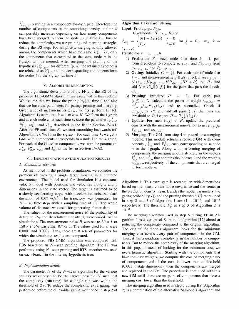
V. ALGORITHM DESCRIPTION

The algorithmic descriptions of the FF and the BS of theproposed FBS-GMM algorithm are presented in this section.We assume that we know the prior p(x0) at time 0 and alsothat we have the parameters for gating, pruning and merging.Given a set of measurements Z1:K , we first perform FF (cf.Algorithm 1) from time k = 1 to k = K. We form the f-graphand at each node n, at each time k, store the parameters µf

k,n,P fk,n, wf

k,n and Ifk,n described in the list in Section IV-A1.After the FF until time K, we start smoothing backwards (cf.Algorithm 2). We form the s-graph. For each time k, we get aGM, with components corresponds to a node l in the s-graph.For each of the Gaussian components, we store the parametersµsk,l, P

sk,l, w

sk,l and Isk,l in the list in Section IV-A2.

VI. IMPLEMENTATION AND SIMULATION RESULTS

A. Simulation scenario

As mentioned in the problem formulation, we consider theproblem of tracking a single target moving in a clutteredenvironment. The model used for simulation is a constant-velocity model with positions and velocities along x and ydimensions in the state vector. The target is assumed to bea slowly accelerating target with acceleration noise standarddeviation of 0.07 m/s2. The trajectory was generated forK = 40 time steps with a sampling time of 1 s. The wholevolume of the track was used for generating clutter data.

The values for the measurement noise R, the probability ofdetection PD and the clutter intensity β, were varied for thesimulations. The measurement noise R was set to 50 × I or150× I . PD was either 0.7 or 1. The values used for β were0.0001 and 0.0002. Thus, there are 8 sets of parameters forwhich the simulation results are compared.

The proposed FBS-GMM algorithm was compared withFBS based on an N−scan pruning algorithm. The FF wasperformed using N−scan pruning and RTS smoother was usedon each branch in the filtering hypothesis tree.

B. Implementation details

The parameter N of the N−scan algorithm for the varioussettings was chosen to be the largest possible N such thatthe complexity (run-time) for a single run was within thethreshold of 2 s. To reduce the complexity, extra gating wasperformed before the ellipsoidal gating mentioned in step 2 of

Algorithm 1 Forward filteringInput: Prior: µ0|0, P0|0.

Likelihoods: H , zk,j , R and

βk,j =

{β(1− PDPG) j = 0

PD j 6= 0, for j = 0, . . .mk, k =

1, . . .K.Iterate for k = 1, . . . ,K

1) Prediction: For each node i at time k − 1, per-form prediction to compute µk|k−1,i and Pk|k−1,i fromµk−1|k−1,i and Pk−1|k−1,i.

2) Gating: Initialize G = {}. For each pair of node i atk− 1 and measurement zk,j ∈ Zk, check if wLL,(i,j) =N(zk,j ; Hµk|k−1,i, HPk|k−1,iH

T +R)> PG and

add G = G⋃{(i, j)} for the pairs that pass the thresh-

old.3) Pruning: Initialize P = {}. For each pair

(i, j) ∈ G, calculate the posterior weight wk,(i,j) =

wfk−1,iβk,jwLL(i, j) and re normalize. Check if

wk,(i,j) > P fP and add all pairs (i, j) that pass the

threshold to P , i.e., set P = P⋃{(i, j)}.

4) Update: For each (i, j) ∈ P , update the predicteddensity with the measurement innovation to get µk,(i,j),Pk,(i,j) and wk,(i,j).

5) Merging: The GM from step 4 is passed to a mergingmodule. This module returns a reduced GM with com-ponents µf

k,n and P fk,n, each corresponding to a node

n in the f-graph. Along with performing merging ofcomponents, the merging module also returns the vectorsIfk,n and wf

k,n that contains the indexes i and the weightswk,(i,j), respectively, of the components that are mergedto form node n.

Algorithm 1. This extra gate is rectangular, with dimensionsbased on the measurement noise covariance and the center atthe prediction density mean. Besides the model parameters, thegating probability PG and the pruning threshold P f

P mentionedin step 2 and 3 of Algorithm 1 are (1 − 10−5) and 10−4

respectively. The threshold P sP in step 3 of Algorithm 2 is

10−3.

The merging algorithm used in step 5 during FF in Al-gorithm 1 is a variant of Salmond’s algorithm [12] aimed atreducing the complexity compared to the original algorithm.The original Salmond’s algorithm looks for the minimummerging cost across every pair of components in the GM.Thus, it has a quadratic complexity in the number of compo-nents. But to reduce the complexity of the merging algorithm,in this paper, instead of looking for the minimum cost, weuse a heuristic algorithm. Starting with the components thathave the least weights, we compute the cost of merging pairsof components and if the cost is lower than a threshold(0.001 × state dimension), then the components are mergedand replaced in the GM. The procedure is continued with thisnew GM until there are no pairs of components that have amerging cost lower than the threshold.

The merging algorithm used in step 5 during BS (Algorithm2) is a combination of the alternative Salmond’s algorithm and

Algorithm 2 Backward smoothing of FBS-GMM

Input: Filtering GM parameters: µfk,n, P f

k,n, wfk,n, Ifk,n, for

n = 1, . . . ,Mfk .

Initialize: Set MsK, =Mf

K , µsK,l = µf

K,l, PsK,l = P f

K,l, IsK,l =

l and wsK,l =

∑rwf

K,l(r) (summation is over the entire vector

wfK,l).

Iterate for k = K − 1, . . . , 1

1) RTS: For each node p at time k+1 in the s-graph, formpairs, (p, n), as described in Section IV-B. Calculatethe smoothing density mean µk|K,(p,n) and covariancePk|K,(p,n) using RTS on µf

k,n, P fk,n and µs

k+1,p, P sk+1,p

(Note, the parameters µsk+1,p and P s

k+1,p are the samefor different n’s).

2) Weight calculation: For each pair (p, n), the weightwk|K,(p,n) is calculated as in (16). After this, we have abunch of triplets

{µk|K,(p,n), Pk|K,(p,n), wk|K,(p,n)

}that

form a GM.3) Pruning: Pruning can be performed on the GM based on

wk|K,(p,n) > P sP after which the GM is re-normalized.

4) Grouping: The components in the pruned GM are sortedinto groups Gn such that all the components in the grouphave a common parent n at time k− 1. The grouping isperformed across all p’s.

5) Merging: Merging can be performed within eachgroup Gn. The output of this merging module is{µsk,l, P

sk,l, w

sk,l

}along with the parameter Isk,l = n.

Runnalls’ algorithm [11]. The additional Runnalls’ algorithmis necessary to ensure that the number of components in theGM during BS is within a threshold (50 components).

The performance measures used for comparison are theRMSE, NEES, complexity and track loss. A track was con-sidered lost if the true state was more than three standarddeviations (obtained from the estimated covariance) away fromthe estimated state for five consecutive time steps. The trackloss was calculated only on the BS results. The complexityresults presented is the average time taken during MATLABsimulations on an Intel i5 at 2.5GHz to run each algorithmon the entire trajectory of 40 time steps. The graphs wereobtained by averaging over 1000 Monte Carlo iterations.

C. Results

The results of the simulations are presented in Fig. 6 to9. It can be seen that the FBS-GMM performs significantlybetter than the FBS with N−scan pruning for most of thescenarios. From the Fig. 6 for track loss performance, onecan notice that the performance gain is higher for FBS-GMMcompared to FBS with N−scan pruning when PD is low andthe measurement noise R and the clutter intensity β are high(point 6 on the x-axis in Fig. 6). The reason for this is thatin these scenarios, the number of components in the filteringGMs before approximations is quite large. To limit the numberof components, the pruning during FBS with N−scan pruningcan be quite aggressive resulting in the degeneracy problem.

Fig. 6: Track Loss. Every odd point on x-axis (1,3,5,7) is for low clutterintensity β = 0.0001 and every even point (2,4,6,8) is for high β =0.0002. The order of the eight scenarios is the same for the others plotsin Fig. 7, Fig. 8 and Fig. 9.

Fig. 7: NEES performance: Compared to the N−scan based FBS, thevalues of the NEES for the FBS-GMM are very close to the optimalvalue of 4 in all the scenarios.

The impact of this degeneracy problem can also be observedin the NEES performance plot in Fig. 7 (point 6 on the x-axis).In the degeneracy case, the uncertainties are underestimated,i.e., the estimated covariances are smaller compared to theoptimal, resulting in a larger value for the NEES comparedto the expected value of 4. In addition to the better track lossand NEES performances, FBS-GMM offers a computationallycheaper solution compared to the FBS based on N−scanpruning as can be observed in Fig. 8. However, the RMSEperformance of the two algorithms are very similar in mostscenarios, as seen in Fig. 9.

VII. CONCLUSION

In this paper, we presented an algorithm for forward-backward smoothing on single-target Gaussian mixtures(GMs) based on a merging algorithm. The weight calculationof the components in the GM during filtering and smoothingwere explained by defining hypotheses. Evaluations of root-mean squared error and track loss were performed on a

Fig. 8: Computational complexity: The FBS-GMM algorithm is compu-tationally cheaper compared to the FBS with N−scan.

Fig. 9: RMSE performance: The results are very similar for the both theFBS algorithms.

simulated scenario. The results showed improved performanceof the proposed algorithm compared to forward-backwardsmoothing on an N−scan pruned hypothesis tree, for lowcomplexity and high credibility (normalized estimation errorsquared).

REFERENCES

[1] I. J. Cox and S. L. Hingorani, “An efficient implemen-tation of Reid’s multiple hypothesis tracking algorithmand its evaluation for the purpose of visual tracking,”IEEE Transactions on Pattern Analysis and MachineIntelligence, vol. 18, no. 2, pp. 138–150, 1996.

[2] D. Crouse, P. Willett, K. Pattipati, and L. Svensson,“A look at gaussian mixture reduction algorithms,” inProceedings of the Fourteenth International Conferenceof Information Fusion, 2011, pp. 1–8.

[3] A. Doucet and A. M. Johansen, “A tutorial on particlefiltering and smoothing: Fifteen years later,” Handbookof Nonlinear Filtering, vol. 12, pp. 656–704, 2009.

[4] O. E. Drummond, “Multiple target tracking with multipleframe, probabilistic data association,” in Optical Engi-neering and Photonics in Aerospace Sensing. Interna-tional Society for Optics and Photonics, 1993, pp. 394–408.

[5] P. Fearnhead, D. Wyncoll, and J. Tawn, “A sequentialsmoothing algorithm with linear computational cost,”Biometrika, vol. 97, no. 2, pp. 447–464, 2010.

[6] D. Fraser and J. Potter, “The optimum linear smootheras a combination of two optimum linear filters,” IEEETransactions on Automatic Control, vol. 14, no. 4, pp.387–390, 1969.

[7] S. J. Godsill, A. Doucet, and M. West, “Monte carlosmoothing for nonlinear time series,” Journal of theAmerican Statistical Association, vol. 99, no. 465, 2004.

[8] W. Koch, “Fixed-interval retrodiction approach tobayesian imm-mht for maneuvering multiple targets,”IEEE Transactions on Aerospace and Electronic Systems,vol. 36, no. 1, pp. 2–14, 2000.

[9] H. Rauch, F. Tung, and C. Striebel, “Maximum likeli-hood estimates of linear dynamic systems,” AIAA Jour-nal, vol. 3, pp. 1445–1450, 1965.

[10] D. Reid, “An algorithm for tracking multiple targets,”IEEE Transactions on Automatic Control, vol. 24, no. 6,pp. 843–854, 1979.

[11] A. R. Runnalls, “Kullback-Leibler approach to Gaussianmixture reduction,” IEEE Transactions on Aerospace andElectronic Systems, vol. 43, no. 3, pp. 989–999, 2007.

[12] D. Salmond, “Mixture reduction algorithms for point andextended object tracking in clutter,” IEEE Transactionson Aerospace and Electronic Systems, vol. 45, no. 2, pp.667–686, 2009.

APPENDIX AWEIGHT CALCULATION

The weight calculation in (11) can be obtained using thehypotheses definitions. Consider the hypothesis expressionin (10), and the illustration in Fig. 5. We are interested incalculating the probability of the hypothesis

Pr{H

′sk,(p,n)|Z1:K

}= Pr

{Hs

k+1,p

⋂Hf

k,n|Z1:K

}∝ Pr

{Hs

k+1,p|Z1:K

}Pr{Hf

k,n|Hsk+1,p, Z1:k+1

}×p(Zk+2:K |Hs

k+1,p,Hfk,n, Z1:k+1). (12)

In the above equation, the factor Pr{Hs

k+1,p|Z1:K

}is the

weight wsk+1,p, which is available from the last iteration of BS

at time k + 1. With respect to the third factor, the followingset of equations show that it is actually independent of n:

p(Zk+2:K |Hsk+1,p,H

fk,n, Z1:k+1)

= p(Zk+2:K |Hsk+1,p,H

fk+1,m,H

fk,n, Z1:k+1) (13)

=

ˆp(xk+1|Hs

k+1,p,Hfk+1,m,H

fk,n, Z1:k+1)

×p(Zk+2:K |Hsk+1,p,H

fk+1,m,H

fk,n, Z1:k+1, xk+1) dxk+1

=

ˆp(xk+1|Hf

k+1,m, Z1:k+1)p(Zk+2:K |Hsk+1,p, xk+1) dxk+1.

(14)

In (13), adding the hypothesis Hfk+1,m to the conditional

statement does not make a difference as the hypothesis Hsk+1,p

corresponding to the entire sequence of measurements masksit; but it does make the latter equations simpler to handle. Thesecond factor in (12) is given by

Pr{Hf

k,n|Hsk+1,p, Z1:k+1

}= Pr

{Hf

k,n|Hfk+1,m, Z1:k+1

}∝

Pr{Hf

k,n,Hfk+1,m|Z1:k+1

}Pr{Hf

k+1,m|Z1:k+1

} . (15)

The numerator term in (15) is the same as the probabilitywf

k+1,m(r) of the rth branch before merging to form node m.Consolidating (14) and (15) into (12), we get that

Pr{H

′sk,(p,n)|Z1:K

}∝ ws

k+1,p × wfk+1,m(r). (16)