Mercator Ocean newsletter 33
43
Mercator Ocean Quarterly Newsletter #33– April 2009 – Page 1 GIP Mercator Ocean Quarterly Newsletter Editorial – April 2009 Left panel: Global mean sea level derived from multiple ocean satellite altimeter missions (Credits: AVISO). Right panel: The Niño3.4 SST anomaly index is an indicator of central tropical Pacific El Niño conditions (Credits: NOAA/PMEL). Greetings all, This month’s newsletter is devoted to ocean indices aiming at a better understanding of the state of the ocean climate. Ocean climate indices can be linked to major patterns of climate variability and usually have a significant social impact. The estimation of the ocean climate indices along with their uncertainty is thus crucial: It gives an indication of our ability to measure the ocean. It is as well a useful tool for decision making. Ocean climate indices also provide an at-a-glance overview of the state of the ocean climate, and a way to talk to a wider audience about the ocean observing system. Several groups of experts are now working on various ocean indicators using ocean forecast models, satellite data and reanalysis models in observing system simulation experiments, among which the OOPC, NOAA and MERSEA/Boss4Gmes communities for example: http://ioc3.unesco.org/oopc/state_of_the_ocean/index.php http://www.cpc.ncep.noaa.gov/products/analysis_monitoring/enso_advisory/ http://www.aoml.noaa.gov/phod/cyclone/data/method.html http://www.mersea.eu.org/Indicators-with-B4G.html Scientific articles about Ocean indices in the present Newsletter are displayed as follows: The first article by Von Schuckmann et al. is dealing with the estimation of global ocean indicators from a gridded hydrographic field. Then, Crosnier et al. are describing the need to conduct intercomparison of model analyses and forecast in order for experts to provide a reliable scientific expertise on ocean climate indicators. The next article by Coppini et al. is telling us about ocean indices computed from the Mediterranean Forecasting System for the European Environment Agency and Boss4Gmes. Then Buarque et al. are revisiting the Tropical Cyclone Heat Potential Index in order to better represent the ocean heat content that interacts with Hurricane. The last article by
-
Upload
mercator-ocean -
Category
Environment
-
view
247 -
download
0
Transcript of Mercator Ocean newsletter 33

Mercator Ocean Quarterly Newsletter #33– April 2009 – Page 1
GIP Mercator Ocean
Quarterly Newsletter
Editorial – April 2009
Left panel: Global mean sea level derived from multiple ocean satellite altimeter missions (Credits: AVISO). Right panel: The Niño3.4 SST anomaly index is an indicator of central tropical Pacific El Niño conditions (Credits: NOAA/PMEL).
Greetings all,
This month’s newsletter is devoted to ocean indices aiming at a better understanding of the state of the ocean climate. Ocean climate indices can be linked to major patterns of climate variability and usually have a significant social impact. The estimation of the ocean climate indices along with their uncertainty is thus crucial: It gives an indication of our ability to measure the ocean. It is as well a useful tool for decision making. Ocean climate indices also provide an at-a-glance overview of the state of the ocean climate, and a way to talk to a wider audience about the ocean observing system. Several groups of experts are now working on various ocean indicators using ocean forecast models, satellite data and reanalysis models in observing system simulation experiments, among which the OOPC, NOAA and MERSEA/Boss4Gmes communities for example:
http://ioc3.unesco.org/oopc/state_of_the_ocean/index.php
http://www.cpc.ncep.noaa.gov/products/analysis_monitoring/enso_advisory/
http://www.aoml.noaa.gov/phod/cyclone/data/method.html
http://www.mersea.eu.org/Indicators-with-B4G.html
Scientific articles about Ocean indices in the present Newsletter are displayed as follows: The first article by Von Schuckmann et al. is dealing with the estimation of global ocean indicators from a gridded hydrographic field. Then, Crosnier et al. are describing the need to conduct intercomparison of model analyses and forecast in order for experts to provide a reliable scientific expertise on ocean climate indicators. The next article by Coppini et al. is telling us about ocean indices computed from the Mediterranean Forecasting System for the European Environment Agency and Boss4Gmes. Then Buarque et al. are revisiting the Tropical Cyclone Heat Potential Index in order to better represent the ocean heat content that interacts with Hurricane. The last article by
Mercator Ocean Quarterly Newsletter #33– April 2009 – Page 2
GIP Mercator Ocean
Greiner et al. is dealing with the assessment of robust ocean indicators and gives an example with oceanic predictors for the Sahel precipitations.
The next July 2009 newsletter will review the current work on data assimilation and its techniques and progress for operational oceanography.
We wish you a pleasant reading.
Contents Estimating Global Ocean indicators from a gridded hydrographic field during 2003‐2008 ............................... 3
By Karina von Schuckmann, Fabienne Gaillard and Pierre-Yves Le Traon
Intercomparison of environmental Ocean indicators: a complementary step toward scientific expertise and
decision making. ......................................................................................................................................... 11
By Laurence Crosnier, Marie Drévillon, Silvana Ramos Buarque, Jean-Michel Lellouche, Eric Chassignet, Ashwanth Srinivasan, Ole Martin Smedstad, Sanjay Rattan and Allan Wallcraft
Mediterranean Marine environmental indicators from the Marine Core Service .......................................... 18
By Giovanni Coppini, Vladyslav Lyubartsev, Nadia Pinardi, Claudia Fratianni, Marina Tonani, Mario Adani, Paolo Oddo and Srdjan Dobricic, Rosalia Santoleri, Simone Colella and Gianluca Volpe
Tropical Cyclone Heat Potential Index revisited ........................................................................................... 24
By Silvana Ramos Buarque, Claude Vanroyen and Caroline Agier
Assessment of robust Ocean indicators: an example with oceanic predictors for the Sahel precipitations. ... 31
By Eric Greiner and Marie Drevillon
0BNotebook .................................................................................................................................................... 43

Mercator Ocean Quarterly Newsletter #33 – April 2009 – Page 3
Estimating Global Ocean indicators from a gridded hydrographic field during 2003-2008
Estimating Global Ocean indicators from a gridded hydrographic field during 2003-2008
By Karina von Schuckmann 1, Fabienne Gaillard 2 and Pierre-Yves Le Traon 1 1 IFREMER (LOS), Brest, France 2 IFREMER (LPO), Brest, France
Abstract
Monthly gridded fields of temperature and salinity of the upper 2000m depth are obtained by optimal analysis of the large in-situ dataset provided by the Argo array of profiling floats, drifting buoys, CTDs and moorings over the period 2003-2008. These fields are used to analyze large-scale and deep variability patterns on interannual time scales during the 6 years of measurements with the substantial advantage that this study is based on a single and uniform data base. Global and basin wide averages of ocean indicators such as heat storage anomalies, freshwater content and steric height have been estimated from the gridded monthly field. We find global average rates of 0.77±0.11Wm-2 for heat storage, 700±1600km3/a for freshwater content and 1.01±0.13 mm/a for steric sea level. The horizontal distribution of these ocean indicators shows largest variability of heat storage and steric height in the North Atlantic Ocean, in the northern tropical Pacific and in the South Pacific. Freshwater content changes from 2003 to 2008 are dominant in the tropical and subtropical basins of the global oceans and are dominated by interannual fluctuations. Variability patterns of steric and total sea level are in good agreement between 30°S-50°N during the 6 years of measurements.
Introduction
Investigating the fluctuations of ocean temperature and salinity properties on interannual to long time scales is essential to understand the oceans role within the climate system. Fluctuations of the hydrographic field occur on all time scales, from which long-term changes and trends are known to be related to atmospheric and anthropogenic forcings. During the past 50 years the world upper ocean has warmed [Levitus et al., 2005], but this warming is not uniformly distributed across the globe [Barnett at al., 2005]. The global warming trend is largely caused by warming in the Atlantic and Southern Ocean [Willis et al., 2004; Levitus et al., 2005; Sallée et al., 2008]. Owing to a lack of salinity observations, previous analyses on interannual to long-term changes of salinity are often limited to regional findings, but large-scale coherent freshening and salinification are observed in all ocean basins [e.g. Antonov et al., 2002; Curry et al., 2003; Boyer et al., 2005, Delcroix et al., 2007, Böning et al., 2008]. However, it is vital to further investigate global hydrographic changes. The monthly gridded measurements as used in this study deliver a uniform description of its changes within the first decade of the 21st century and produce especially for the salinity field a global estimation of its fluctuations.
Indeed systematic errors persist in the global monitoring systems and it is essential to draw attention to this matter. In a global study of heat content on the basis of in-situ profile data two different instrument biases have recently be discovered caused by a small fraction of Argo floats type SOLO FSI and eXpantable Bathy-Thermographs (XBTs) [Willis et al., 2009]. After the detection of these errors, updates of ocean heat content for the upper 700m of the world ocean are delivered by Levitus et al., 2009. However, systematic long-period errors remain in the observing systems [Willis et al., 2008]. Only small contributions of these biases can induce large signatures in global estimates of ocean indicators such as heat content, steric sea level and freshwater content. Thus, extracting these parameters from the global observing system is a useful tool to detect systematic errors. Evaluating these indicators from the gridded in-situ measurements on a regular basis and compare its results with previous findings and other datasets such as satellite derived measurement will shed more light on the sensitivity of the observing systems and offers information on the state of the global ocean. Here we present a short description of the dataset. Then we further discuss different ocean indicators, i.e. heat storage anomalies, freshwater content and steric sea level as derived from the monthly gridded field of temperature and salinity. Changes of steric sea level will be also compared with total sea level as provided by satellite altimetry. Conclusions are given in the final section.
Data analysis method
Monthly gridded fields of temperature and salinity from the surface down to 2000m depth are obtained by optimal analysis of a global field of in-situ measurements (Coriolis data center) during the years 2003-2008 under the French project ARIVO (http://www.ifremer.fr/lpo/arivo). This data field is based on the Argo array of profiling floats (95% of the data, see http://www.argo.net), drifting buoys, shipboard measurements and moorings. A small fraction of observations has been excluded from the analysis due to existing instrument biases as discussed above, i.e. gray-listed Argo floats of type SOLO FSI and XBTs. The gridding method is derived from estimation theory [Liebelt, 1967; Bretherton et al., 1976] and the method itself is described in detail by Gaillard et al., 2008 and will be not discussed in this context. The analyzed field is defined on a horizontal ½° Mercator

Mercator Ocean Quarterly Newsletter #33 – April 2009 – Page 4
Estimating Global Ocean indicators from a gridded hydrographic field during 2003-2008
isotropic grid and is limited from 77°S to 77°N. The vertical resolution between the surface and 2000m depth is gridded onto 152 vertical levels. The reference field is the monthly World Ocean Atlas 2005 [WOA05, Locarnini et al., 2006; Antonov et al., 2006]. The statistical information on the field is gained from the a priori covariance of the field at every grid point (Figure 1a and b). Further discussion on the statistical description can be found in von Schuckmann et al. (2009). However, as seen in Figure 1a and b, the data coverage of temperature and salinity is not uniformly distributed in space and is accumulated in regions of previous research interest. In the tropical basin for example, it is higher for temperature in the upper layer because of the TAO/Pirata mooring arrays. In the western north Pacific and North Indian Ocean the percentage of a priori variance is lower due to intense deployments of Argo floats. Slight deficit in Argo profiles occur in the Atlantic Ocean since profiler of type SOLO FSI are excluded from the analysis. It can be summarized that the best estimation is obtained between 30°S and 50°N. The data coverage of temperature and salinity strongly decreases below 1000m depth, but increases from the year 2003 to the end of 2008 [von Schuckmann et al., 2009].
Figure 1
Horizontal map of percent of a priori variance for a) temperature and b) salinity at 100m depth. The percentage of a priori variance is averaged in time from 2003-2008. A 100% of a priori variance indicates that no information is gained from the measurement
field.

Mercator Ocean Quarterly Newsletter #33 – April 2009 – Page 5
Estimating Global Ocean indicators from a gridded hydrographic field during 2003-2008
Global ocean heat storage anomalies
Changes in ocean heat storage anomalies from 2003 to 2008 are derived from the monthly gridded temperature field and averaged globally as well as over every single ocean basin (Figure 2a). The anomalies are relative to the mean seasonal cycle derived from the gridded temperature field during 2003-2008 and the heat storage anomaly is calculated as done by Levitus et al. (2005) from the surface down to 2000m depth. In the global mean (Figure 2a, black line), a considerable warming is visible from the year 2003 to 2008 with an average warming rate of 0.77±0.11Wm-2. In the analysis of Willis et al. (2004) using satellite altimeter height combined with in-situ temperature profiles in the upper 700m depth an oceanic warming rate of 0.86±0.12Wm-2 is estimated from mid-1993 through mid-2003. Their warming rate is higher compared to our estimation indicating that either changes in the 750-2000m depth layer or interannual and decadal changes contribute to the average warming. Levitus et al. (2005) have shown that the world ocean heat content from the surface down to 3000m depth has increased at a rage of 0.2Wm-2. Since their estimation is based on in-situ data over an earlier and much longer time period this value is much lower. As already suggested by the same authors, much of this increase in heat content comes from the Atlantic (Figure 2a, red), which shows an average rate of 1.55±0.33Wm-2 during the six years of measurements. The Indian Ocean warms at a rate of 0.83±0.35Wm-2
during 2003-2008. The lowest rate can be observed in the Pacific Ocean since there strong interannual fluctuations (La Niña in 2007) lead to large cooling patterns in that basin (Figure 2b). Regional cooling occurs also in the southern Indian Ocean and at northern mid-latitudes in the Pacific and Atlantic Ocean. Largest signatures of 6-year warming can be observed in the North Atlantic Ocean. Moreover, warming signatures also occur in the tropical Atlantic and at southern mid-latitudes. Warming in the Indian Ocean is limited to the southern hemisphere tropics and subtropics. In the Pacific Ocean, warming is dominant in the western part of the basin, especially in the tropics and at southern mid-latitudes.
Figure 2
a) Time series of global mean heat storage anomalies (0-2000m) as well as averaged over the Pacific (blue), Atlantic (red) and Indian (green) Ocean basin in Jm-2, together with its average linear trends in mm/year. b) Horizontal map of heat storage changes
from 2003 to 2008 in Wm-2.

Mercator Ocean Quarterly Newsletter #33 – April 2009 – Page 6
Estimating Global Ocean indicators from a gridded hydrographic field during 2003-2008
Global equivalent freshwater content
Monthly gridded salinity measurements in the upper 2000m depth are used to evaluate equivalent freshwater content as defined by Boyer et al. (2007), relative to a ARIVO salinity climatology during 2003-2008. This method is valid under the assumption that the salt content is relatively constant over the analysis time and that any changes in salinity are due to the addition or subtraction of freshwater to the water column – including vertical movements of the isopycnal surfaces and convection processes. Many mechanisms can lead to the addition or subtraction of freshwater, e.g. air-sea freshwater flux, river runoff, sea-ice formation as well as storage of freshwater in continental glaciers. However, here we present the signature of freshwater content on global scales (Figure 3). The global and thus, the basin wide averages are dominated by interannual fluctuations during the years 2003-2008 (Figure 3a) and significant rates can only be observed in the Atlantic and Pacific Ocean. A significant increase in salinity occurs in the Atlantic, predominantly in the southern tropics and subtropics, but also evidence exists in the eastern North Atlantic (Figure 2b). In the analysis of Boyer et al. (2007) a decrease in freshwater can be observed for the North Atlantic during a much longer time period, i.e. from 1955 to 2003. Also freshening signatures appear in the 6-year changes in the Atlantic basin, which are concentrated in the northern tropics and northwestern subtropics as well as in the Southern Ocean. The freshening in the Pacific can be more attributed to decadal or longer-term changes as indicated by the time series in Figure 3a (blue line). The entire basin is characterized by freshening signatures during 2003-2008, except in the eastern North Pacific and in the areas of the tropical convergence zones (Figure 3b). Largest deep freshening occurs south of Australia [e.g. Antonov et al., 2002; Böning et al., 2008], as well as in the eastern tropics. Large 6-year changes of freshwater content persist also in the Indian Ocean, mostly at lower periods (Figure 3a). Basin-wide bands of altering sign dominate the freshwater fluctuations in the Indian Ocean from its northern extend to the southern subtropics. At southern mid-latitudes, a large-scale freshening can be observed which is constistent with previous results (e.g. Morrow et al., 2008).
Figure 3
Same as Figure 2, but for freshwater content (0-2000m) in km3 and in km3/year for its linear trends.

Mercator Ocean Quarterly Newsletter #33 – April 2009 – Page 7
Estimating Global Ocean indicators from a gridded hydrographic field during 2003-2008
Global steric height
Monthly values of steric height are derived from the gridded temperature and salinity field as described by Gilson et al. (2002) from the surface down to 1500m depth. The globally averaged steric sea level during 2003-2008 shows a positive trend and the rate of 6-year changes can be estimated as 1.01±0.13 mm/a (Figure 4a). The 6-year changes based on the steric contribution alone constitutes about 40% to the total sea level rise during that time [von Schuckmann et al., 2009]. Low-period fluctuations exist in the time series but are small compared to the long-term variability. The largest contribution of 6-year sea level rise occurs in the Indian Ocean with an average rate of 1.39±0.45 mm/a, predominantly due to positive anomalies in the western tropical and subtropical Indian Ocean and within the South Equatorial Current (SEC) extend (Figure 4b and c). Indeed, warming of the Indian Ocean during 2003-2008 is significantly high, but also salinity plays an important role in the Indian Ocean. For example, beside the 6-year increase of steric sea level, a warming and increase in salinity arises within the SEC (Figure 2b and 3b). The average rate of steric height in the Atlantic Ocean accounts for 1.00±0.23 mm/a, and much of this increase can be attributed to changes in the subtropical and subpolar gyres, as well as in the South Atlantic (Figure 4b and c). The lowest rate exists in the Pacific Ocean due to the large signature of interannual variability during the 6 years of measurements. The comparison of total and steric sea level in Figure 4b and c indicate that good agreement occurs within 50°N-30°S, i.e. the area where a good estimation is achieved as discussed in the data description. Six-year changes of steric sea level are generally lower and largest differences occur in some areas of the Indian and Pacific Ocean, i.e. in areas where ocean variability is governed by a barotropic response of the ocean to wind forcing (Guinehut et al., 2006). Regional differences can be also observed in the tropical and southern subtropical Indian Ocean, although the data coverage is high for both, temperature and salinity measurements (Figure 1a and b).

Mercator Ocean Quarterly Newsletter #33 – April 2009 – Page 8
Estimating Global Ocean indicators from a gridded hydrographic field during 2003-2008
Figure 4
a) & b) same as Figure 2, but for steric height (0-1500m) in cm and in mm/year for its linear trends. c) Same as b), but using total sea level from AVISO (merged gridded product (1/4°), delayed mode, www.aviso.oceanobs.com).
Conclusion
Here we present results from a global hydrographic data product based on in-situ temperature and salinity measurements during the years 2003-2008 in the upper 2000m depth of the world ocean. Global and basin wide averages of ocean indicators such as heat storage anomalies, freshwater content and steric height have been estimated from the gridded monthly field. We find global average rates of 0.77±0.11Wm-2 for heat storage, 700±1600km3/a for freshwater content and 1.01±0.13 mm/a for steric sea level. Similar to previous findings, the warming rate is strongest in the Atlantic Ocean which is accompanied by a strong increase of steric height. Freshwater content is dominated by interannual fluctuations in that basin. Largest positive 6-year changes of all three parameters occur predominantly in the subtropical and subpolar gyre systems of the Atlantic Ocean. The hydrographic

Mercator Ocean Quarterly Newsletter #33 – April 2009 – Page 9
Estimating Global Ocean indicators from a gridded hydrographic field during 2003-2008
changes in the Pacific Ocean are dominated by the strong La Niña event in the year 2007. In the South Pacific, large areas of warming, freshening and steric sea level rise can be observed during 2003-2008. In the Indian Ocean, meridional changes of alternating sign arise in all three parameters, which is especially visible in the freshwater content changes. In this basin, differences between total sea level and its steric contribution are largest, mainly in the tropics and in the SEC extend. Beside this discrepancy, horizontal patterns of steric height and total sea level changes during 2003-2008 are in good agreement between 30°S-50°N.
Recently, the Argo array is fully developed and produces a uniform monitoring of the global ocean, thus reducing errors caused by undersampling and revealing consistent and accurate estimates of the ocean state. The sensitivity of ocean indices with respect to different types of measurements (different instruments) and the data processing needs to be tested. However, to detect systematic errors in the observing system it is important to analyze ocean indicators on global and regional scales and compare those to other datasets and previous findings which is the objective of present and future research of Mercator Ocean and Coriolis.
Acknowledgements
This work was supported by an IFREMER grant and the European project BOSS4-GMES.
References
Antonov, J., S. Levitus, and T. Boyer, 2002: Steric sea level variations during 1957-1994: Importance of salinity, J. Geophys. Res., 107, doi: 10.1029/2001JC000964.
Antonov J., R. Locarnini, T. Boyer, A. Mishonov and H. Garcia, 2006: World Ocean Atlas 2005, Volume 2: Salinity, S. Levitus, ED., NOAA Atlas NESDIS, U.S. Government Printing Office, Washington D.C., 182-184.
Barnett, T., D. Pierce, K. AchutaRao, P. Gleckler, B. Santer, J. Gregory and W. Washington, 2005: Penetration of human-induced warming into the world’s oceans, Science, 309, 284-287.
Böning, C., A. DIspert, M. Visbeck, S. Rintoul and F. Schwarzkopf, 2008: The response of the Antarctic Circumpolar Current to recent climate change, Nature, doi: 10.1038/ngeo362.
Boyer, T., S. Levitus, J. Antonov, R. Locarnini, and H. Garcia, 2005: Linear trends in salinity for the World Ocean, 1955-1998, Geophys. Res. Lett., 32, doi: 10.1029/2004GL021791.
Boyer, T., S. Levitus, J. Antonov, R. Locarnini, A. Mishov, H. Garcia and S. Josey, 2007 : Changes in freshwater content in the North Atlantic Ocean 1955-2006, Geophys. Res. Lett., 34, doi: 10.1029/2007GL030126.
Boyer, T., S. Levitus, J. Antonov, R. Locarnini, A. Mishonov, H. Garcia and S.A. Josey, 2007 : Changes in freshwater content in the North Atlantic Ocean 1955-2006, Geophys. Res. Lett., 34, doi: 10.1029/2007GL030126.
Bretherton, F., R. Davis and C. Fandry, 1976: A technique for objective analysis and design of oceanic experiments applied to Mode-73, Deep-Sea Res., 23, 559-582.
Curry, R., B. Dickson and I. Yashayaev, 2003: A change in the freshwater balance of the Atlantic Ocean over the past four decades, Letters to Nature, 426, 826-829.
Delcroix, T., S. Cravatte and J. McPhaden, 2007 : Decadal variations and trends in tropical Pacific sea surface salinity since 1970, J. Geophys. Res., 112, doi: 10.1029/2006JC003801.
Gaillard, F., E. Autret, V. Thierry, P. Galaup, C. Coatanoan and T. Loubrieu, 2008: Quality control of large Argo data sets, J. Atmos. Ocean. Tech., 26, 337-351, doi: 10.1175/2008JTECHO552.1.
Gilson J., D. Roemmich, B. Cornuelle and L.-L. Fu, 1998: Relationship of TOPEX/Poseidon altimetric height to steric height and circulation in the North Pacific, J. Geophys. Res., 103, 27,947-27,965.
Guinehut, S., P.-Y. Le Traon and G. Larnicol, 2006: What can we learn from Global Altimetry/Hydrography comparisons?, Geophys. Res. Lett., 33, doi: 10.1029/2005GL025551.
Levitus, S., J. Antonov and T. Boyer, 2005: Warming of the World Ocean, 1955-2003, Geophys. Res. Lett., 32, doi: 10.1029/2004GL021892.
Levitus, S., J.I. Antonov, T.P. Boyer, R.A. Locarnini, H.E. Garcia and A.V. Mishonov, 2009: Global Ocean Heat Content 1955-2008 in light of recently revealed instrument problems, Geophys. Res. Lett., accepted.
Liebelt, P., 1967: An introduction to optimal estimation, Addison-Welsey, 267-269.

Mercator Ocean Quarterly Newsletter #33 – April 2009 – Page 10
Estimating Global Ocean indicators from a gridded hydrographic field during 2003-2008
Locarnini, R., A. Mishonov, J. Antonov, T. Boyer and H. Garcia, 2006: World Ocean Atlas 2005, Volume 1: Temperature, S. Levitus, ED., NOAA Atlas NESDIS, U.S. Government Printing Office, Washington D.C., 182-184.
Morrow, R., G. Valladeau and J.-B. Salee, 2008: Observed subsurface signature of Southern Ocean sea level rise, Prog. Oceanogr., 77, 351-366.
Sallèe, J., R. Morrow and K. Speer, 2008: Southern Ocean fronts and their variability to climate modes, J. Clim, 21, 3020-3039.
von Schuckmann, K., F. Gaillard and P.-Y. Le Traon, 2009: Global hydrographic variability patterns during 2003-2008, J. Geophys. Res., accepted.
Willis, J., D. Roemmich and B. Cornuelle, 2004: Interannual variability in upper ocean heat content, temperature, and thermosteric expansion on global scales, J. Geophys. Res., 109, doi: 10.1029/2003JC002260.
Willis, J., J. Lyman, G. Johnson and J. Gilson, 2009: In Situ Data Biases and Recent Ocean Heat Content Variability, J. Atmos. Ocean. Technol., doi: 10.1175/2008JTECHO608.1.
Willis, J., D. Chambers and R. Nerem, 2008, Assessing the globally averaged sea level budget on seasonal to interannual time scales, J. Geophys. Res., 113, doi: 10.1029/2007JC004517.

Mercator Ocean Quarterly Newsletter #33 – April 2009 – Page 11
Intercomparison of environmental Ocean indicators
Intercomparison of environmental Ocean indicators: a complementary step toward scientific expertise and decision making. By Laurence Crosnier 1, Marie Drevillon 1, Silvana Ramos Buarque 1, Jean-Michel Lellouche 1, Eric Chassignet 2, Ashwanth Srinivasan 2, Ole.Martin Smedstad 3, Sanjay Rattan 2 and Allan Wallcraft 3 1 Mercator Ocean, Ramonville St Agne, France 2 Center for Ocean-Atmospheric Prediction Studies (COAPS), FSU, Tallahassee, FL,USA 3 Naval Research Lab, Stennis Space Center, MS,USA
Abstract
A large range of Ocean operational systems are operated in various forecasting centers, able to analyze and forecast the ocean state, including 3D ocean temperature, salinity and currents at various horizontal and vertical resolutions. Ocean climate indicators are computed using observations and the latter numerical ocean analyses and forecasts. It is the combination of observations as well as model derived ocean climate indicators and of human scientific expertise that allows stating on the ocean climate. Two strategies are usually followed by the experts: either a multi model/observations approach or a choice of one model (or one observations data set) result among several when they know it performs better than the others. In order to figure out which one of the two strategies to choose, each model prognostic variable (i.e: 3D ocean temperature, salinity and currents, sea level anomaly) skills have to be assessed and an intercomparison of the ocean climate indicators in the various Ocean Forecast System (henceforth OFS) has to be undertaken. In the present paper, two global OFS are used: the Mercator OFS operated at Mercator-Ocean, France and the HYCOM OFS operated at the Stennis Space Center, MS, USA. Three classical environmental indicators based on upper layer ocean temperature are computed with those two OFS. We show that even though ocean temperature skills for each individual OFS are well known, an intercomparison of the ocean climate indicators is a complementary step for the scientific expertise.
Introduction
Ocean environmental indicators provide information for a better understanding of the oceans and their ecosystems, as well a simple representation of ocean climate variability. A strong scientific expertise is required in order to analyze the computed ocean indicators and help the decision making. In particular, when interpreting the results of a physical model (computational method or numerical model) one has to take into account its known strengths and weaknesses. State-of-the-art Ocean General Circulation Models (OGCM) like NEMO or HYCOM are very efficient to describe the ocean state, especially thanks to data assimilation techniques. In the mean time, they are very complicated (even more when advanced data assimilation techniques are used) and include a lot of parameterizations which can interact to create biases. If those biases are difficult to control and reduce, at least they are usually well identified and monitored. It is hence the combination of model numerical results and of human scientific expertise that allows stating on the ocean climate. For example, groups of experts are gathering regularly in order to state on the El Nino phenomenon in the USA (http://www.cpc.noaa.gov/products/analysis_monitoring/enso_advisory/index.shtml), as well as in France (Ramos Buarque et al. 2007). Experts either take a multi model approach, or choose one model results among several when they know this specific model is performing better than the others in the considered area or for the considered season or a specific physical process.
In the framework of MyOcean (http://www.myocean.eu.org/) and GODAE (http://www.godae.org/), several forecasting centers are operating a large range of operational systems (Ocean Forecast System, henceforth OFS) able to analyze and forecast the ocean state including the 3D ocean temperature, salinity and currents at various resolutions. Intercomparison of the prognostic variables (i.e: 3D ocean temperature, salinity and currents, sea level anomaly) of those various systems has been conducted within the framework of MERSEA (http://www.mersea.eu.org/) (Crosnier and LeProvost 2006) and GODAE, in order to put in light the strength and weaknesses of each OFS. The present paper rather presents an intercomparison of ocean indicators (i.e. diagnostic variables) in order to help Ocean experts figuring out which strategy to choose (either a multi-model approach merging all the available OFS, or the one OFS choice approach).
The present paper is intercomparing indicators computed from two global OFS: The Mercator OFS operated at Mercator-Ocean, Toulouse, France and the HYCOM OFS operated at Stennis Space Center, MS, USA. We first briefly present the two OFS. We then intercompare the ocean environmental indicators based on a computation using the upper layer ocean temperature in the two OFS: an upwelling index based on the Sea Surface Temperature, the Coral Bleaching indicators and the Tropical Cyclone Heat Potential showing the thermal energy available in the ocean to enhance or decrease the power of cyclones. Finally we briefly discuss the results and conclude.

Mercator Ocean Quarterly Newsletter #33 – April 2009 – Page 12
Intercomparison of environmental Ocean indicators
Description of the two global Ocean Forecasting Systems (OFS)
The Mercator OFS
Mercator-Ocean is operating the Mercator Global Ocean ¼° OFS with a higher 1/12° resolution in the Atlantic Ocean and Mediterranean Sea with 50 vertical levels [NEMO ocean code (Madec et al., 1998)], with assimilation [multivariate assimilation scheme with 3D control vector: (T, S, U, V and Hbar) with SEEK kernel and 3D error covariance modes] of Sea Level Anomaly (ENVISAT + JASON + GFO + RIOv5 MSSH), Sea Surface Temperature (RTG-SST from NCEP) and temperature and salinity in situ profiles (Coriolis). The sea ice is fully comprehensive with the implementation of the LIM2 model with sea ice concentration, sea ice/snow thickness, sea ice drift and sea ice thermal content. Weekly runs provide daily mean analysis and forecast fields. Surface forcings are computed from ECMWF atmospheric analyses (bulk formulae). The OFS is started from Levitus climatology in October 2006, and from a sea ice climatology derived from a NEMO ¼° experiment.
The Hycom OFS
The Stennis Space Center is operating the HYCOM Global Ocean 1/12° OFS with 32 hybrid layers [HYCOM 2.2], with assimilation [NCODA multivariate assimilation scheme with 3D control vector (T, S, U, V, and P)] of Sea Level Anomaly (ENVISAT + JASON + GFO), Sea Surface Temperature (AVHRR + Microwave), SSMI sea ice concentration and temperature and salinity in situ profiles (XBTs, ARGO, moorings, and buoys). A thermodynamic (energy loan) sea ice is implemented. Surface forcing are coming from the NOGAPS surface atmospheric fields using bulk formula, with 986 rivers and a weak relaxation to climatological Sea Surface Salinity. The model started with a 5-year spinup from the GDEM climatology and is then turned into the assimilation mode from 2003 to present.
Intercomparison of Environmental Ocean indicators
In this section, we intercompare various ocean environmental indicators computed in the Mercator and HYCOM OFS.
Upwelling Index
Figure 1
Location along the French, Spanish and Portuguese coast of the cyan and red dots used to compute surface temperature differences for upwelling Index. Background color represents the Sea Surface Temperature (ºC) in the Mercator OFS on July 22
2008.
Mercator Ocean Quarterly Newsletter #33 – April 2009 – Page 13
Intercomparison of environmental Ocean indicators
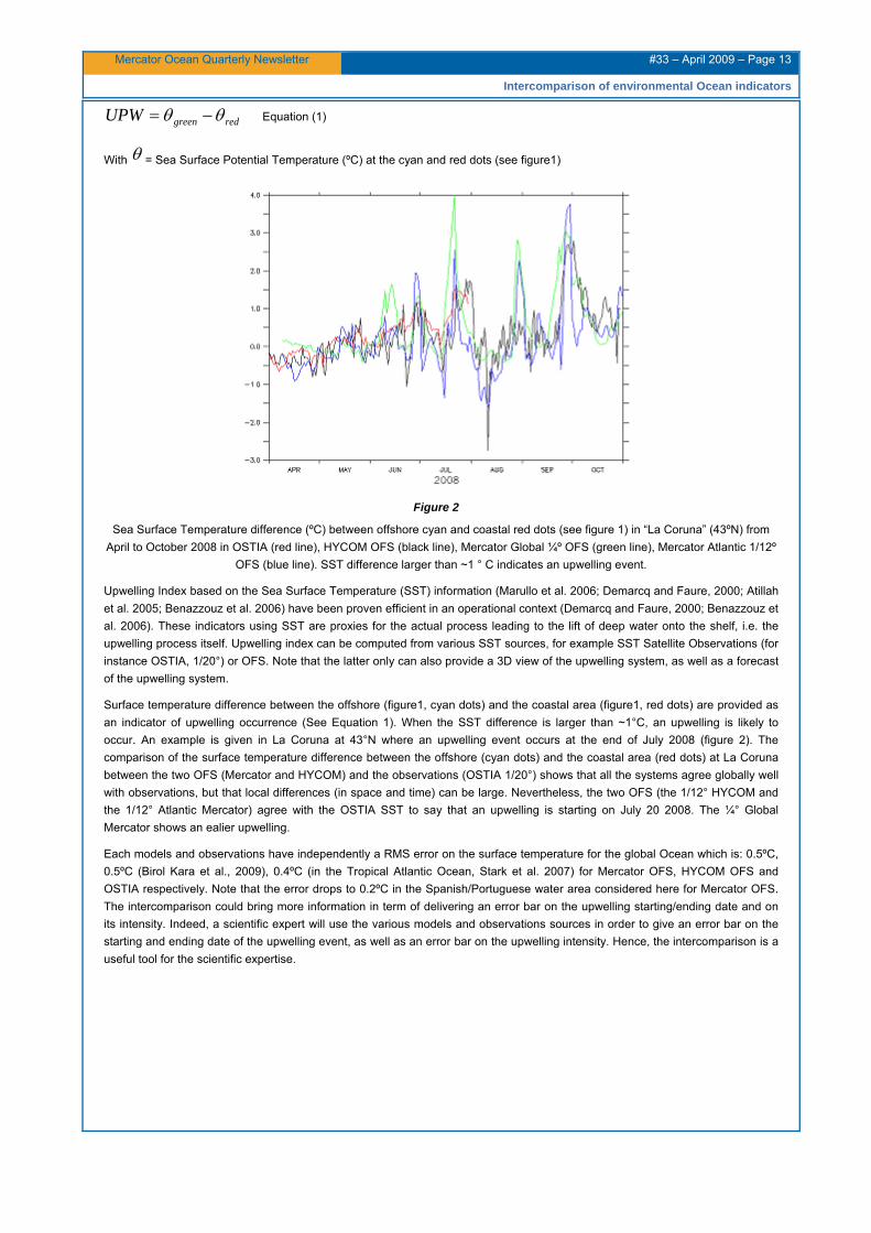
redgreenUPW θθ −= Equation (1)
With θ = Sea Surface Potential Temperature (ºC) at the cyan and red dots (see figure1)
Figure 2
Sea Surface Temperature difference (ºC) between offshore cyan and coastal red dots (see figure 1) in “La Coruna” (43ºN) from April to October 2008 in OSTIA (red line), HYCOM OFS (black line), Mercator Global ¼º OFS (green line), Mercator Atlantic 1/12º
OFS (blue line). SST difference larger than ~1 ° C indicates an upwelling event.
Upwelling Index based on the Sea Surface Temperature (SST) information (Marullo et al. 2006; Demarcq and Faure, 2000; Atillah et al. 2005; Benazzouz et al. 2006) have been proven efficient in an operational context (Demarcq and Faure, 2000; Benazzouz et al. 2006). These indicators using SST are proxies for the actual process leading to the lift of deep water onto the shelf, i.e. the upwelling process itself. Upwelling index can be computed from various SST sources, for example SST Satellite Observations (for instance OSTIA, 1/20°) or OFS. Note that the latter only can also provide a 3D view of the upwelling system, as well as a forecast of the upwelling system.
Surface temperature difference between the offshore (figure1, cyan dots) and the coastal area (figure1, red dots) are provided as an indicator of upwelling occurrence (See Equation 1). When the SST difference is larger than ~1°C, an upwelling is likely to occur. An example is given in La Coruna at 43°N where an upwelling event occurs at the end of July 2008 (figure 2). The comparison of the surface temperature difference between the offshore (cyan dots) and the coastal area (red dots) at La Coruna between the two OFS (Mercator and HYCOM) and the observations (OSTIA 1/20°) shows that all the systems agree globally well with observations, but that local differences (in space and time) can be large. Nevertheless, the two OFS (the 1/12° HYCOM and the 1/12° Atlantic Mercator) agree with the OSTIA SST to say that an upwelling is starting on July 20 2008. The ¼° Global Mercator shows an ealier upwelling.
Each models and observations have independently a RMS error on the surface temperature for the global Ocean which is: 0.5ºC, 0.5ºC (Birol Kara et al., 2009), 0.4ºC (in the Tropical Atlantic Ocean, Stark et al. 2007) for Mercator OFS, HYCOM OFS and OSTIA respectively. Note that the error drops to 0.2ºC in the Spanish/Portuguese water area considered here for Mercator OFS. The intercomparison could bring more information in term of delivering an error bar on the upwelling starting/ending date and on its intensity. Indeed, a scientific expert will use the various models and observations sources in order to give an error bar on the starting and ending date of the upwelling event, as well as an error bar on the upwelling intensity. Hence, the intercomparison is a useful tool for the scientific expertise.

Mercator Ocean Quarterly Newsletter #33 – April 2009 – Page 14
Intercomparison of environmental Ocean indicators
Coral bleaching
Figure 3
Global Ocean Coral bleaching HotSpot (ºC) (left panels) and Global Ocean Coral bleaching Degree of Heating Weeks (units=°C-weeks) (right panels) on July 28 2008 from NOAA (top panel), Mercator Global ¼º OFS (middle panel) and HYCOM OFS (bottom
panel).
Coral bleaching is a serious threat to coral reefs worldwide and mass coral bleaching is most often caused by elevated SST. The need for improved understanding, monitoring, and prediction of coral bleaching has become imperative. Coral bleaching monitoring and assessment products include 2 main indices: coral bleaching HotSpots, coral bleaching Degree Heating Weeks (DHW) which definition can be found on the following websites http://www.osdpd.noaa.gov/PSB/EPS/SST/climohot.html and http://coralreefwatch.noaa.gov/satellite/methodology/methodology.html#hotspot. Both indices are computed using Sea Surface Temperature information.
Coral bleaching Hotspot and Degree Heating Weeks spatial structure location in Mercator and HYCOM OFS agree well with the NOAA ones (figure 3). Nevertheless, local geographical differences can be sometimes large and both Mercator and HYCOM Hotspot values are weaker than the NOAA ones at mid-latitudes. This has to be further investigated, but might be due to the different climatology used in the NOAA (1985-1993 climatology of MCSSTs from RSMAS) versus HYCOM / Mercator computation. The HYCOM OFS (1/12º) is giving smaller scale information than the Mercator coarser global resolution (1/4º) OFS. The main input from an OFS versus a SST satellite observation is its forecast capacity (2 weeks ahead for the Mercator OFS).
Again, the RMS error on the surface temperature for the global ocean are: 0.5ºC, 0.5ºC (Birol Kara et al., 2009), <0.5ºC for Mercator OFS, HYCOM OFS and NOAA/NESDIS SSTs respectively. The intercomparison is bringing more information in term of delivering an error bar on the location of the spatial patterns of the coral bleaching HotSpots and Degree Heating Weeks and on the intensity of each pattern. Hence, the intercomparison is a useful tool for the scientific expertise.

Mercator Ocean Quarterly Newsletter #33 – April 2009 – Page 15
Intercomparison of environmental Ocean indicators
Tropical Cyclone Heat Potential
Figure 4
Tropical Cyclone Heat Potential (TCHP) (kJ cm-2) (Left panels) and Depth of the 26°C isotherm (metres) (D26, right panels) on July 30 2008 from NOAA (top panel), Mercator Global ¼º OFS (middle panel) and HYCOM OFS (bottom panel).

Mercator Ocean Quarterly Newsletter #33 – April 2009 – Page 16
Intercomparison of environmental Ocean indicators
Figure 5
Tropical Cyclone Heat Potential (TCHP) (kJ cm-2) in the Gulf of Mexico with superimposed the track of hurricane Gustav on
September 1st 2008 (color dots and numbers indicate cyclone category) from NOAA (left panel), Mercator Atlantic 1/12º OFS
(middle panel) and HYCOM OFS (right panel).
Tropical Cyclone Heat Potential (TCHP) is defined as a measure of the integrated vertical temperature from the sea surface to the depth of the 26°C isotherm (Leipper and Volgenau, 1972, Goni and Trinanes 2003, Shay et al. 2000) (see equation 2 below).
[ ]dzCTCHPD
p ∫ −=0
26
26θρ Equation (2) with pCρ = 4.09 106 J K-1 m-3
There is a great interest in the hurricane modeller community for realistic TCHP products, because coupling hurricane forecast models to ocean models allows them to take into account the influence of TCHP on hurricane behaviour. Hence, realistic ocean-model products are needed.
The NOAA TCHP is computed from altimeter-derived vertical temperature-profile estimates in the upper ocean, i.e vertical profiles derived from altimeter surface observations. Mercator and HYCOM OFS directly derive the TCHP from the prognostic 3D variables of the ocean numerical models that are run in real time, and which are constrained by the altimeter data. Hence, the main input from OFS versus altimeter satellite observations for TCHP computation is that OFS provide more precise information about the upper-ocean 3D vertical thermal structure, with the great advantage of TCHP predictions two weeks ahead.
Globally, the maximum TCHP areas of Mercator are in better agreement with the NOAA estimation than HYCOM, especially in the Western tropical Pacific (see example with figure 4 on July 30 2008) where TCHP values are larger in Mercator than in HYCOM. This is due to shallower D26 (i.e. Depth of the 26°C isotherm) in HYCOM than in Mercator and NOAA (figure 4). It has to be further investigated why the HYCOM D26 is shallower than Mercator and NOAA estimates.
In the case of Hurricane Gustav on Sept 1st 2008 (figure 5), HYCOM and Mercator with a similar 1/12º horizontal resolution give a similar TCHP global structure with nevertheless large local mesocale structure differences. In the case where the HYCOM and Mercator OFS were coupled to a hurricane forecast model, those large mesoscale structures difference would be likely to impact the hurricane track forecast. In this case, it has to be further investigated which approach is best to compute the TCHP: either to consider all 3 TCHP estimates (for example using an ensemble mean of NOAA, HYCOM and Mercator estimates) or to choose one of them for example.
The intercomparison is bringing more information in terms of delivering an error bar on the location of the spatial patterns of TCHP and on the intensity of each pattern. Again, the intercomparison can be a useful tool for the scientific expertise.

Mercator Ocean Quarterly Newsletter #33 – April 2009 – Page 17
Intercomparison of environmental Ocean indicators
Conclusion
In the present paper, two global OFS are used: the Mercator OFS operated at Mercator-Ocean, France and the HYCOM OFS operated at the Stennis Space Center, MS, USA. Three classical environmental indicators based on upper layer ocean temperature are computed in those two OFS. We show that even though each OFS skills for ocean temperature are independently well known, an intercomparison of the ocean climate indicators is a necessary step for the scientific expertise. Indeed, space and time differences between Mercator and HYCOM can be locally large for some of the ocean indicators and can change the local/daily interpretation and influence decision making. Further work has to be done computing the level of confidence of each indicator regarding weaknesses and skills of each system. In some cases, experts may want to use one of the 2 systems, and in other cases they may want to use all the available systems. Both approaches will probably be needed in the future.
In a near future, MyOcean is providing Marine Core Services including 3D ocean fields to downstream users in order for them to define for example environmental indicators. In this context, several Ocean 3D reanalysis long time series will also be available for the users to study which combination of ocean incidators can produce the most reliable information on the state of the ocean and the associated environmental risks.
References
Atillah A., Orbi A., Hilmi K., Mangin A., 2005 : Produits opérationnels d’océanographie spatiale pour le suivi et l’analyse du phénomène d’upwelling marocain, GEO OBSERVATEUR n°14, Novembre 2005, p49-62.
Benazzouz A., Hilmi K., Orbi A., Demarcq H., Atillah A., 2006: Dynamique spatio temporelle de l’upwelling cotier Marocain par teledetection de 1985 a 2005, GEO OBSERVATEUR n°15, Novembre 2006.
Birol Kara A., Alan J. Wallcraft, Harley E. Hurlburt and Wei-Yin Lohb, 2009, Quantifying SST errors from an OGCM in relation to atmospheric forcing variables, doi:10.1016/j.ocemod.2009.03.001, Ocean Modelling, Volume 29, Issue 1, 2009, Pages 43-57.
Crosnier L. and C. Le Provost, 2006, Inter-comparing five forecast operational systems in the North Atlantic and Mediterranean basins: The MERSEA-strand1 Methodology, Journal of Marine System, 2006,doi: 10.1016/j.jmarsys.2005.01.003
Demarcq H. and Faure V., 2000: Coastal upwelling and associated retention indices derived from satellite SST. Application to Octopus vulgaris recruitment, OCEANOLOGICA ACTA
Volume 23, 4, pp391-408.
Goni G. J. and J.A. Trinanes, 2003: Ocean thermal structure Monitoring could aid in the Intensity Forecast of Tropical cyclones, EOS, vol. 84, No51, 23 December 2003.
Leipper D and D. Volgenau, 1972: Hurricane heat potential of the Gulf of Mexico, J. Phys. Oceanography, 2, 218-224, 1972.
Madec G., P. Delecluse, M. Imbard, and C. Levy, 1998 : OPA 8.1 general circulation model reference manual, Notes de l'Institut Pierre-Simon Laplace (IPSL) - Université P. et M. Curie, B102 T15-E5, 4 place Jussieu, Paris cédex 5, 91p, (1998).
Marullo S., Ludicone D. and R. Santoleri, 2006: Altimetric data to monitor the seasonal and year-to-year variability of the upwelling intensity along the West Africa coasts, OSTST Ocean Surface Topography Science Team meeting, March 16-18, 2006, Venice, Italy.
Ramos Buarque S., Cassou C., Charon I., Gueremy J.F., 2007, "Bulletin climatique global" of Météo-France: a contribution of Mercator Ocean to the seasonal prediction of El Nino 2006/07. Mercator-Ocean Quarterly Newsletter #26, July 2007, pp19-26.
Shay, L.K., G. J. Goni and P. G. Black, 2000: Effects of Warm Oceanic Features on Hurricane Opal, Month. Weath. Rev., 128, 131-148, 2000.
Stark John D., Craig J. Donlon, Matthew J. Martin and Michael E. McCulloch, 2007, OSTIA : An operational, high resolution, realtime, global sea surface temperature analysis system. http://ghrsst-pp.metoffice.com/pages/latest_analysis/ostia.html

Mercator Ocean Quarterly Newsletter #33 – April 2009 – Page 18
Mediterranean Marine environmental indicator from the Marine Core Service
Mediterranean Marine environmental indicators from the Marine Core Service By Giovanni Coppini 1,2, Vladyslav Lyubartsev 3, Nadia Pinardi 1,2, Claudia Fratianni 1, Marina Tonani 1, Mario Adani 1, Paolo Oddo 1 and Srdjan Dobricic 3, Rosalia Santoleri 4, Simone Colella 4 and Gianluca Volpe 4 1 Istituto Nazionale di Geofisica e Vulcanologia (INGV), Italy 2 Università di Bologna (UNIBO), Italy 3 Centro Euro Mediterraneao per i Cambiamenti Climatici (CMCC), Italy 4 Consiglio Nazionale delle Ricerche Istituto di Scienze dell'Atmosfera e Del Clima (CNR-ISAC), Italy
Abstract
The Mediterranean Forecasting System (Pinardi et al., 2003) has started the design and development of services that include the routine production of environmental and climate indicators. A process of identifying user requirements has been started in collaboration with European Environment Agency and the indicators definition and implementation aim to take user requirements into account. The indicators are extensively used by EEA (EEA web page on indicators: http://themes.eea.europa.eu/indicators/). INGV has carried out an analysis on the possible improvements of existing indicators in use by EEA and on the development of new indicators based on Marine Core Services (MCS) products. The list of indicators includes: Temperature, Chlorophyll-a (from ocean colour), Ocean Currents and Transport, Salinity, Transparency, Sea Level, Sea Ice and Density. A critical analysis has been carried out to identify the relevance of the above-mentioned indicators for EU policies, their spatial and temporal coverage, their accuracy and their availability (Coppini et al., 2008). INGV in collaboration with CNR-ISAC are directly involved in the development of the indicators in the Mediterranean region and the Temperature and Chlorophyll-a (Chl-a) products are the most suitable for an indicator development test phase. In particular the Operational Oceanography (OO) Chl-a product, deduced from satellite data, will be able to contribute to the further development of the EEA Chl-a indicator that is based on in-situ measurements (CSI023). Sea Level and Sea Ice products are also robust quantities for climate indicators. For the above mentioned indicators a development test phase has been undertaken in 2008 within the European Topic Center for Water (ETC-W) and BOSS4GMES (http://www.mersea.eu.org/Indicators-with-B4G.html) projects. In addition to the products mentioned above, we have also identified a Density indicator that appears relevant for the eutrophication problems and ecosystem health.
Introduction
INGV takes part within MyOcean contributing to the implementation of the GMES (www.gmes.info) Marine Fast Track Service, notably the Marine Core Service (MCS) for the protection and management of the marine environment. The different Spatial Data Theme Elements (SDTE) produced by the MCS have been examined in the prospective of contributing to the development of indicators for EEA (Coppini et al, 2008). The SDTE examined are: Temperature, Chlorophyll-a (from ocean colour), Ocean Currents and Transport, Salinity, Transparency, Sea Level, Sea Ice and Density. SDTE are defined following the INSPIRE Directive and are ocean state variables with specified spatial and temporal resolution. The usage of “SDTE” nomenclature should help to distinguish between SDTE such as “Temperature” and the derived set of indicators. For some of the OO SDTE we present the data and products availability (table 1). These STDE are chosen among those indicated by EMMA (European Marine Monitoring and Assessment) (EEA-led EMMA OO Workshop final report, 2006).
Indicators definition and implementation
Indicators provide information on matters of wider significance than what is actually measured or make perceptible a trend or phenomenon that is not immediately detectable (Hammond et al., 1995). Environmental indicators reflect trends in the state of the environment and monitor the progress made in realising environmental policy targets and provide insight into the state and dynamics of the environment (Smeets and Weterings, 1999).
Environmental indicators are synthetic values extracted from a relevant SDTE: they should be subdivided into ranges of values which correspond to the assessment of a qualitative state of the environment. For each examined SDTE (Temperature, Chlorophyll-a (from ocean colour), Ocean Currents and Transport, Salinity, Transparency, Sea Level, Sea Ice and Density) we have proposed a definition and relevant indicator development has started. Here we presented the implementation phase of the indicator that started in ETC-Water and BOSS4GMES for the products
Table 1 presents the indicators and SDTE implemented in BOSS4GMES, in addition in ETC-Water, INGV is working for EEA to develop a new indicator based on ocean color products.

Mercator Ocean Quarterly Newsletter #33 – April 2009 – Page 19
Mediterranean Marine environmental indicator from the Marine Core Service
BOSS4GMES MFS Indicator List
SST Sea Surface Temperature [°C]
SST anomaly Sea Surface Temperature Anomaly [°C]
The difference between the SST of the model and the SST of the Medatlas climatology
(1).
SSS Sea Surface Salinity [PSU]
HC Heat Content [1021J]
Calculated in 0-150 m upper layer by multiplying the volume of water by its density and specific heat capacity.
HC anomaly Heat Content Anomaly [1021J]
The difference between the HC of the model and the HC of the Medatlas climatology1.
Net Volume Transports
Net Volume Transports [Sv]
Calculated for the Strait of Gibraltar, Sicily Channel, and Corsica Channel. Sv = 106
m3/s.
Net Volume Transports Anomaly
Net Volume Transports Anomaly [Sv]
The difference between the Net Volume Transport of the model and the Net Volume Transport of the MFS sys2b climatology2. Calculated for the Strait of Gibraltar, Sicily
Channel, and Corsica Channel. Sv = 106 m3/s.
Table 1
Indicators developed at INGV for the Mediterranean Sea in the framework of BOSS4GMES project.
The indicators are calculated using MFS analysis and forecast and are updated daily and weekly depending on the products. MFS indicators are available at the following web page: http://gnoo.bo.ingv.it/mfs/B4G_indicators/MFS_indicators.htm
The following sections present the definition of indicators and series of examples when available.
Temperature SDTE and indicator
SST products provide high frequency and complete spatial coverage for the global ocean and the regional seas. In-situ surface data are of large importance to validate satellite data and to increase the accuracy of the combined satellite and in-situ dataset and provide, together with model analysis, information on entire water column. Presently EEA is using Sea Surface Temperature timeseries in the Climate change and assessment reports and an indicator related to the Global and European Temperature (CSI 012) exists and shows trends in annual average global and European temperature and European winter/summer temperatures for land and ocean together. Temperature related indicators can answer policy-relevant questions such as: will the global average temperature increase stay within the EU policy target (2 degrees C above pre-industrial levels)? This question is related to the Council Decision (2002/358/EC) of 25 April 2002 and Decision No 280/2004/EC of the European Parliament and of the Council of 11 February 2004.
Different indicators related to the ocean temperature can be derived from the OO temperature SDTE. A first set is related to SST where the longest time series are available (1871-today). The inclusion of regional high resolution satellite datasets for several European Seas started with the 2008 report “Impacts of Europe's changing climate - 2008 indicator-based assessment” (http://www.eea.europa.eu/publications/eea_report_2008_4) and should continue. Additional indicators are possible to be developed that consider the whole water column temperature and that could be indicative of long term effects and extreme events. The latter are very relevant for ecosystems dynamics and possible stresses (Real time SST anomalies maps with time scales from daily to 1 THE MEDAR GROUP - 2002 MEDAR/MEDATLAS 1998-2001 Mediterranean and Black Sea database of temperature, salinity and bio-chemical parameters and climatological atlas (4 CDRoms), European Commission Marine Science and Technology Programme, Centre de Brest. http://www.ifremer.fr/medar/ 2 MFS sys2b climatology is calculated from MFS sys2b model analysis since January 2001 until the last week, and updated weekly.

Mercator Ocean Quarterly Newsletter #33 – April 2009 – Page 20
Mediterranean Marine environmental indicator from the Marine Core Service
monthly, annual basin average Heat Content (HC) anomalies from approximately 1985-today, HC linear trends and maps of the spatial distribution of HC linear trends from 1985-today, real time temperature anomaly profiles in the water column, mixed layer depth anomalies time series).
An example of indicator developed in BOSS4GMES is given for the Temperature indicator in Figure 1. The Mediterranean Sea Surface Temperature anomaly has been calculated using the daily forecast of the Mediterranean Forecasting System compared with the MEDATLAS climatology. Ocean Temperature is relevant for marine ecosystem and for example unusually high summer temperatures were able to impact coastal ecosystems in the Mediterranean. During the summer of 1999, record high temperatures combined with stable water column conditions over a period of several weeks caused physiological stress to benthic fauna and triggered the development of pathogens that otherwise would have remained non-toxic (Cerrano et al 2000, De Bono et al 2004, Garrabou et al 2001, Perez et al 2000, Romano et al 2000). The SST anomaly indicator could be able to detect high SST anomaly.
Figure 1
Mediterranean Sea Surface Temperature anomaly calculated from MFS forecast with respect to MEDATLAS climatology (produced by INGV) http://gnoo.bo.ingv.it/mfs/B4G_indicators/SST_anomaly.htm
Concerning SST, INGV is contributing together with the Global, Arctic, North East Atlantic and Baltic MFC to a visualization services at EEA. A new web page at EEA website has been produced, the web page is composed of two parts:
• The long term change in SST (since 1870) using HADISST1 dataset and also regional high resolution SST datasets for the Mediterranean Sea, North Sea and Baltic Sea. http://www.eea.europa.eu/themes/coast_sea/sea-surface-temperature
• The short term SST behaviour through MyOcean products such as the today forecast of SST for the Global Ocean and the European regional Seas. http://www.eea.europa.eu/themes/coast_sea/todays-sea-surface-temperature
In addition to SST and SST anomaly we also have developed a product related to heat content and heat content anomaly.
Chl-a SDTE and indicator
The SDTE related to Chl-a is a well developed satellite product and it is now widely available at daily and monthly time scales in all European coastal/shelf and open ocean waters (higher temporal resolution can be achieved in southern European regional seas). OO Chl-a products are derived from all available satellite sensors and cover the periods 1980-1986 and 1997 to the present. The former dataset, however, will be difficult to include in the indicators production. The relevant EEA indicator for Chl-a is the CSI023 (Chlorophyll in transitional, coastal and marine waters - Core Set of Indicator n° 023: http://themes.eea.europa.eu/IMS/IMS/ISpecs/ISpecification20041007132031/full_spec ) which evaluate the trends of Chl-a for seasonal (June to September for stations north of 59 degrees in the Baltic Sea (Gulf of Bothnia and Gulf of Finland) and from May to September for all other stations) mean of chl-a from in-situ collected samples, integrated in the first 10 meters. The objective of the CSI023 indicator is to demonstrate the effects of measures taken to reduce discharges of nitrogen and phosphate on coastal concentrations of phytoplankton expressed as chlorophyll-a. This is an indicator of eutrophication. This indicator is relevant for all the EU Directives aimed at reducing the loads and impacts of nutrients (i.e.: Nitrates Directive (91/676/EEC), Urban Waste Water Treatment Directive (91/271/EEC)).
In order to include indicators from Chl-a derived products for Chl-a into the CSI 023, we are studying the different morphological and hydrological structure of European regional areas identifying shelf, coastal and deep ocean water areas and classify them into ‘Chl-a areas’. The new Chl-a indicator could then be: a) Analyses of summer period mean in the different Chl-a areas to detect trends as

Mercator Ocean Quarterly Newsletter #33 – April 2009 – Page 21
Mediterranean Marine environmental indicator from the Marine Core Service
it is done for CSI023, b) Monthly mean anomaly time series of Chl-a averaged in the different coastal, shelf and deep ocean areas of the European seas; c) Spatial and temporal linear trends of Chl-a seasonal and monthly mean anomalies; d) Real time Chl-a anomaly maps (time scale can range from daily to monthly). Moreover intercalibration of CSI 023 indicator with OO Chl-a derived product will be carried out.
Ocean Currents and Transports SDTE and indicator
Ocean Currents and Transports SDTE are now produced by OO allowing for estimation of transboundary currents, water exchanges and residence time. These could be turned into indicators and related to marine ecosystem functioning and changes. In the North Sea/Norwegian Sea such correlation has been shown to be relevant for the size of the horse mackerel stock, but this correlation with environmental and ecosystem aspects is not yet well developed in other European marine areas.
In the framework of BOSS4GMES INGV has implemented a product related to transports at relevant straits (Figure 2) but we still need to work to establish the connection between transport and relevant environmental changes.
Figure 2
Corsica Channel volume net transport anomaly on respect to sys2b MFS model climatology [Sv]. http://gnoo.bo.ingv.it/mfs/B4G_indicators/transports_anomaly.htm
Salinity SDTE and indicator
Salinity SDTE will allow estimating indirectly the changes in evaporation-precipitation, ice sheet and glacier melting and river-run-off (also due to human impacts). Using OO products, salinity indicators could be developed to monitor the changes in salinity all over the European Seas. Several indicators could be developed such as annual and basin average surface salinity anomalies, surface salinity linear trends of the period and maps showing the spatial distribution of salinity linear trends. Moreover real time salinity anomalies maps and real time salinity anomaly profiles in the water column can be produced.
Transparency SDTE and indicator
Water transparency can be estimated with Ocean Colors images by estimating the K (490) values together with and Case I and Case II water flags. Transparency SDTE is suitable to derive indicators in support the water quality monitoring (i.e. European Directive 76/160/EEC on Bathing Water Quality). Similarly to the Chl-a indicators it is recommended to develop transparency indicators based upon the different morphological and hydrological structure of European regional areas, identifying shelf, coastal and deep ocean water areas. The new transparency indicators could then be: a) monthly mean anomaly time series of transparency averaged in the different coastal, shelf and deep ocean areas of the European seas; b) spatial and temporal linear trends of transparency seasonal and monthly mean anomalies; c) real time transparency anomaly maps (time scale can range from daily to monthly).
Sea level SDTE and indicator
This Sea Level SDTE is derived from two main observational data streams: the sea level stations dataset and the satellite altimetry dataset. Whereas the in-situ sea level measurements is a unique mean to provide the longest timeseries of sea level measurements dating back to late 1800, accurate estimation of the sea level trend and its associated spatial structure are estimated for the last 17 years thanks to satellite altimetry. OO has already organized the production and visualization of Sea level trend indicators from altimetry at different space and time scale (AVISO web site: http://www.aviso.oceanobs.com/en/news/ocean-indicators/mean-sea-

Mercator Ocean Quarterly Newsletter #33 – April 2009 – Page 22
Mediterranean Marine environmental indicator from the Marine Core Service
level/index.html). In the past EEA had used only insitu data to estimate sea level trends for the last century. Starting from the last EEA climate change and impacts report EEA has started to include OO altimetry data.
This indicator can also be calculated using MFS re-analysis
Density SDTE and indicator
The ‘stratification-stability’ indicator is a derived quantity from the density profiles deduced from temperature and salinity data and could be calculated using the Brunt-Vaisala frequency which is a measure of stability of the water column. This indicator appears relevant for the eutrophication problems and ecosystem health and can contribute to the Water Framework Directive characterization of coastal waters at pan-European level.
Discussion
Chl-a SDTE appears ready to be used and an indicator development test phase has started. The OO Chl-a STDE, deduced from satellite data, should be able to contribute to the further development of the EEA CSI-23 Chl-a indicator based on in-situ datasets improving its representativeness for European coastal waters.
Temperature SDTE is a mature and multiple source data set in OO. Its estimates come from multiple data sources, such as satellite, in-situ measurements and models. Quality of the OO products for this SDTE is high (most of the time less than 0.5 deg C). SST from OO SDTE products allows a high frequency and complete global to regional coverage and they are of significant value for climate change monitoring. New indicators could be extracted from the deep temperature OO products.
The SST indicator is already in use at EEA and a webpage at EEA website has been created.
It is believed that the Ocean Current and Transport SDTE are less ready for the development of new indicators at pan-European levels because their relationship with environmental and ecosystem aspects is not yet well developed and quantified for all European Seas.
Conclusion
The key SDTEs produced by MCS services are considered mature for contribution to the development of several indicators for EEA. Most of the described SDTEs are contributing to the development of pan-European uniform coverage indicators. This paper has documented the contribution of the Mediterranean Forecasting System and this and should be at the basis of a demonstration exercise to be carried out in 2008 where the indicators are produced by the OO services. The paper identifies Chl-a and Temperature STDE derived indicators as being the most relevant to be implemented. A first example of MFS indicators is given in the following webpage: http://gnoo.bo.ingv.it/mfs/B4G_indicators/MFS_indicators.htm
Acknowledgements
Financial support for our work was provided by the ETC-W consortium (European Topic Center for Water) funded by the European Environment Agency (EEA), the EU project MERSEA (Marine Environment and Security for the European Area, Contract number: SIP3-CT-2003-502885) and BOSS4GMES (Building Operational Sustainable Services for GMES, contract number: FP6-2005-SPACE-1-030966).
We would like to acknowledge the contribution to this work of Dr. Trine Christiansen and Dr. Eva Royo Gelabert from the European Environment Agency and to Anita Kuenitzer coordinator of the ETC-W consortium.
References
Cerrano C., Bavestrello G. Bianchi C. N., Cattaneo-vietti R., Brava S., Morganti C., Morri C. Picco P., Sara G., Schiapparelli S., Siccardi A., Sponga F. (2000). A catastrophic mass-mortality episode of gorgonians and other organisms in the Ligurian Sea (North-western Mediterranean) summer 1999. Ecology Letters 3: 284-293
Coppini G., Pinardi N., Lyubartsev V., Soulat F., Larnicol G., Guinehut S., Pujol I., Johannessen J., Fratianni C., Tonani M., Marullo S., Loewe P., Santoleri R., Colella S. and Volpe G.. Operational Oceanography and European Environment Agency indicators. 2008 EUROGOOS conference proceedings. submitted
De Bono, A., Pedruzzi, P., Giuliani, G., and Kluser, S. (2004). Impacts of summer 2003 heat wave in Europe. Early Warning on Emerging Environmental Threats. UNEP/DEWA/_Europe/GRID-Geneva
Mercator Ocean Quarterly Newsletter #33 – April 2009 – Page 23
Mediterranean Marine environmental indicator from the Marine Core Service
EEA-led EMMA OO Workshop (EEA, Copenhagen, 23-24 October 2006): “Connecting operational oceanography with the European Marine Strategy and EEA assessments“ – Final report: http://circa.europa.eu/Public/irc/env/marine/library?l=/workingsgroups/europeansmarinesmonitori/eea-led_2006-2007/operational_oceanography/4_-_report/final_201206pdf/_EN_1.0_&a=d
EEA Report No 4/2008, Impacts of Europe's changing climate - 2008 indicator-based assessment, http://www.eea.europa.eu/publications/eea_report_2008_4
Garrabou J., Perez T., Sartoretto S., Harmelin J. G.. (2001) Mass mortality event in red coral Corallium rubrum populations in the Provence region (France, NW Mediterranean). MARINE ECOLOGY PROGRESS SERIES Vol. 217: 263–272, 2001
Hammond, A., Adriaanse, A., Rodenburg, E., Bryant, D., Woodward, R. (1995). Environmental indicators: a systematic approach to measuring and reporting on environmental policy performance in the context of sustainable development. World Resources Institute, Washington, DC.
Perez T., Garrabou J., Sartoretto S, Harmelin J.-G., Francour P., Vacelet J. (2000). Mortalité massive d’invertébrés marins un événement sans précédent en Méditerranée nord-occidentale. C.R. Acad. Sci. Paris, Sciences de la vie / Life Sciences 323 (2000) 853–865
Pinardi, N., I. Allen , E. Demirov, P. De Mey, G.Korres, A.Lascaratos, P-Y. Le Traon, C.Maillard, G. Manzella, C. Tziavos, The Mediterranean ocean Forecasting System: first phase of implementation (1998-2001), Annales Geophysicae, 21: 3-20 (2003).
Romano J.-C., Bensoussan N, Younes W. A.N., Arlhac D. (2000) Anomalie thermique dans les eaux du golfe de Marseille durant l’été 1999. Une explication partielle de la mortalité d’invertébrés fixés ? C.R. Acad. Sci. Paris, Sciences de la vie / Life Sciences 323 (2000) 415–427
Smeets, E., Weterings, R. (1999). Environmental Indicators: Typology and Overview. Technical Report 25, European Environment Agency, Copenhagen (http://reports.eea.eu.int:80/TEC25/en/tech 25 text.pdf ).
Mercator Ocean Quarterly Newsletter #33 – April 2009 – Page 24
Tropical Cyclone Heat Potential Index revisited
Tropical Cyclone Heat Potential Index revisited By Silvana Ramos Buarque 1, Claude Vanroyen 2 and Caroline Agier 3 1 Mercator-Ocean, Ramonville Sainte Agne, France 2 Météo-France, Nouméa, Nouvelle Calédonie 3 Météo-France, Paris, France
Abstract
The aim of this study is to assess the low and the high frequency variability of the Mercator-Ocean Global Ocean Forecast System (MERCATOR) at the time of the Tropical Cyclone (TC) passage in order to evaluate its potential to provide an ocean indicator of TC intensity for real time use.
A new MERCATOR indicator quantifying the heat content available in the Ocean Mixed Layer (OML) is compared to the MERCATOR Tropical Cyclone Heat Potential (TCHP). The cross correlation between the atmospheric pressure and MERCATOR indicator is quantified respectively for the days D:D and D:D-1. The difference between the correlation coefficient for D:D and D:D-1 related to MERCATOR TCHP is not significant because the TCHP is associated with the low frequency heat content of the ocean. On the contrary, the MERCATOR indicators quantifying the heat content available in the OML shows that the correlation coefficient for D:D-1 is twice larger than D:D.
An event-driven evaluation of the MERCATOR indicator was made for each oceanic basin. Results show that for all basins a strong value of the MERCATOR indicator is followed by a decrease of the atmospheric pressure and thus by the increase of the TC intensity.
Note that while the TCHP quantifies the heat content contained between the sea surface and the 26ºC isotherm depth, the MERCATOR indicator quantifies the heat content available in the OML. In the case where the atmospheric surface forcing is not to some extent in agreement with the observed ones, the MERCATOR indicator is able to retrieve the low frequency heat content of the ocean. When the surface forcing is realistic the MERCATOR indicator can be used as a powerful predicator for TC intensification. Otherwise, when the surface forcing is not realistic a very useful MERCATOR TCHP preserves an acceptable level of predictability related to the low frequency heat content.
This result highlights the added value of MERCATOR indicators for the TC intensity forecast as independent estimates or for cross expertise taking into account satellite derived observations and/or numerical air-sea coupled models.
Introduction
In this work a Tropical Cyclone (TC) is a generic name for a “non-frontal synoptic scale low-pressure system over tropical or sub-tropical waters with organized convection (i.e. thunderstorm activity) and definite cyclone surface wind circulation” (McBride et al., 2006; Holland, 1993). The term TC concerns all basins and all intensities including specific appellations as Hurricanes and Typhoons.
Climatically and globally the regions of TC genesis respond to changes on an interannual scale (Chu, 2005). On this scale and only in the North Atlantic there is a well established positive relationship between the Sea Surface Temperature (SST) impact and both frequency and intensity of TC. At mesoscale several works relating to different basins have shown that the TC weakens if the SST falls below 26° (Sinclair et al., 2002; DeMaria and Kaplan, 1994; Gadgil et al., 1984). The Tropical Cyclone Heat Potential (TCHP) - defined by the heat content integrated between the surface and the depth of the isotherm 26°C (Leipper and Volgenau, 1972) - is used to investigate the upper ocean thermal structure from altimeter to monitor the intensity of TC (Goni and Trinanes, 2003). The sensitivity of TC intensity to Ocean Mixed Layer (OML) structure which depends on the strength of the mean flow has been also examined (Samson et al., 2008; Chan et al., 2001). When the transfer of momentum at the air-sea interface by strong wind-current entrains cold waters from the thermocline into the ML depth a reduction of the turbulent surface heat and moisture fluxes is verified. This transfer depends on spatial distribution of the wind and translation speed. These studies show that the TC passage change the vertical structure of the ocean.
This work examine the potential of Mercator-Ocean Global Ocean Forecast System (MERCATOR) to contributes to the TC intensity forecast as an indicator and/or independent estimates for cross expertise taking into account satellite derived observations and/or numerical air-sea coupled models.
In this study, MERCATOR uses the ocean model based on the code OPA 8.2 at the resolution ¼° (Madec et al., 1998), assimilates available satellite altimetry observations and is forced with atmospheric conditions supplied by ECMWF (European Centre for Medium-range Weather Forecasts) (Drévillon et al., 2006). MERCATOR is launched weekly providing daily mean outputs. Thus, the MERCATOR ocean heat content interacts with the TC forecasted by the atmospheric model. The

Mercator Ocean Quarterly Newsletter #33 – April 2009 – Page 25
Tropical Cyclone Heat Potential Index revisited
MERCATOR native grid is interpolated into regular grids which are 1/2° for the global domain and of 1/4° and 1/6° for tropical and sub-tropical regions respectively.
The MERCATOR TCHP
The MERCATOR ability to simulate TCHP in relationship with TC intensification is shown by processing a point-to-point cross correlation (method of least squares) between the atmospheric pressure (Pa) and the oceanic variables TCHP, 26° isotherm Depth (D26), SST and OML (Ramos-Buarque and Landes, 2008). The Pa is predicted from satellite observations in the center of TC. The informations concerning the TC (localization, speed, Pa, etc.) comes from Météo-France by a warming e-mail following the WMO procedure.
Table 1 shows the correlation coefficients in % for global and regional grids. For the regional grid, mostly of TC is positioned in the North Atlantic and North West Pacific. The correlation coefficient remains stable for all variables showing that MERCATOR in upper ocean thermal structure is reliable thanks to the surface altimeter data which constrain the model thermodynamics (Crosnier et al., 2007). The weak differences between the correlation coefficients related to global and regional grids suggests that a part of the ocean that influence the TC intensification is not in connection with the spatial detail of structures.
Variables TCHP SST OML Grid
Pa 14 13 13 1/4° and 1/6°
Pa 17 15 13 1/2° Table 1
The point-to-point cross-correlation coefficients in % between the atmospheric pressure (Pa) and the MERCATOR interpolated variables into regular grids which are of 1/2° for the global domain and of both 1/4° and 1/6° for tropical and sub-tropical
regions.
A delayed cross correlation between Pa for the day D and ocean variables for the day D-1 was also processed. The correlations
related to D:D takes into account 119 days (points) (Table 1) whereas those related to D:D-1 takes into account 60 days. The delayed correlation coefficient between Pa and TCHP is 11% whereas the correlation coefficient for D:D is of 14%. The difference between the correlation coefficients for D:D and D:D-1 is not significant because the TCHP is associated with low frequency heat content.
The MERCATOR indicators
The interaction between the atmosphere and the ocean concerns processes of surface and sub-surface. The intensity of the winds on the surface and the transfer of the kinetic energy from the cyclone towards the ocean operate modifications on its source of energy. Moreover, some parameters concerning the upper ocean thermal structure has been shown to play an important role in TC intensity. However, it seems that these oceanic parameters taken separately are not preponderant in the intensification of the TC but rather a derived quantity like a gradient along the trajectory from the TC (Goni and Trinanes, 2003).
In order to calculate precisely the quantity of thermal energy available in the ocean it is necessary to determine the thickness of the oceanic layer interacting with the atmospheric phenomenon. The processes which can trigger the mixing of the upper ocean are numerous. One of these processes is the friction, due to the winds on the surface where the production of kinetic energy is important. Another processes is the “Ekman pumping” which results in displacement of the thermocline caused by the divergence of the currents on the surface. The thermocline can move due to the mixing and upwelling of waters, as well as to the uptake of thermal energy by the TC. On the point of view of model estimates the OML which can move easily coincides with the thermal OML. Beyond this depth, the variations in temperature become a physical barrier where the mixing collapses. In order to overshoot the barrier it will be necessary to spend a great quantity of energy to destabilize the thermal stratification.
Thus, the thermal energy contained in the OML is seen as the energy easily assimilated by the TC. In agreement with the climatological studies carried out on this domain, only the heat content contained in sea waters with temperature higher than 26°C is taken into account.
The eye of a TC is the calmest region generally with a diameter from 20 to 60 km on the sea surface. The subsidence of the stratospheric air is responsible of the relatively dry (no precipitations) and hot air anomaly. The temperatures are of 10 to 15°C larger than in its environment. Around this area, the “wall of the eye” has a very dense cloudy mass surrounding the center of the TC with a radius of the order of 150 km with strong winds. The “core region” is delimited by the “wall of the eye”. Away from this core region the wind speed falls off gradually. Thus, the core of the TC is the region where the exchange with the

Mercator Ocean Quarterly Newsletter #33 – April 2009 – Page 26
Tropical Cyclone Heat Potential Index revisited
atmosphere is maximum and mostly due to the evaporation which participates strongly to the cooling of the sea waters. In the formulation of the new indicator of TC intensities, the exchanges with the atmosphere are taken into account in the “core of the TC”.
The potential thermal energy interacting with the TC (Interacting Tropical Cyclone Heat Content, ITCHC) is defined by the surface integral of the thermal energy favorable to the intensification of the Cyclone contained in the OML following the relationship:
( ) ( ) θρθπ
θ
rdrdTCrITCHCCMOz
z
p
r
r∫ ∫∫= ==
⎥⎦
⎤⎢⎣
⎡−=
2
0
)(
00
dz 26.,*
(1)
where r* is the radius corresponding to the circle of strong winds taken as 150 km, the density ρ was taken as 1025 kg.m-3 and the specific heat Cp was taken as 3900 J.kg-1.deg-1. The term (T-26) is the temperature difference above 26C for the MERCATOR OML.
Otherwise, the approximate thermal energy loss by the ocean at a given location can be estimated from direct measurements before and after the TC (Leipper, 1967). It appears that the exchange rate is of the order of 4000 cal.cm-².day-1, or ten times the exchange rate in normal weather situations. Thus, based on the relation (1) an Indicator of Cyclonic Celerity (ICC) is defined as the ratio between the thermal energy contained in the OML in the zone of strong winds and the thermal energy which should release an equivalent surface to ensure the maintenance of the cyclonic activity (Vanroyen et Agier, 2008a). This indicator takes the following form:
refFSITCHC
yxICC *),( = (2)
where S* is the surface which the TC is considered to be in interaction with. This surface is selected as being the averaged circle of strong winds. Fref is the daily contribution of thermal energy necessary to maintain the TC activity and is approximately equal to 17 kJ.cm-² per day (or close to 4000 cal.cm-².jour-1). The ICC was calculated for 26 TC from MERCATOR corresponding to the cyclonic seasons going from January 2007 to June 2008.
Thus, while the TCHP quantifies the heat content contained between the sea surface and D26, the ITCHC quantifies the heat content available in the OML. The cross correlations were carried out between Pa and the averaged ITCHC over the inner circle of the TC related to the upper ocean heat loss primarily due to the wind stress. The correlation coefficients for D:D and D:D-1 are respectively 22% and 42%.
An event-driven validation was made for each oceanic basin (Figures 1, 2 and 3). Each case illustrates the intensity of the TC related to the ICC. The intensity of the TC is seen through Pa related to the ICC. In addition, the TC trajectory as well as its category is superimposed on the SST fields.
A code color was adopted: The locations of the centre of TC which seemed problematic because of an obvious interaction with the terrestrial surfaces are shown with translucent color. In red, definitively excluded points and in green the points for which an interaction with the ground is probable.
In the Pacific basin (Figure 1) the ICC are maximum from the first day and a notable fall of the atmospheric pressure appears. Over the following days precisely from D3 to D5 the ICC remain stable (around 1.5) the atmospheric pressure varies little. Then, between D6 and D7, a clear reduction of the ICC is followed by a clear increase in the atmospheric pressure between D7 and D8. Finally, the ICC for D8 is strong enough and the decrease in the atmospheric pressure between D8 and D9 is obvious. The TC FUNA is also a good example of the ICC robustness. As soon as the TC appears it evolves on strongly energetic surfaces and once again a strong value of the ICC is followed by a decrease of the atmospheric pressure and thus by the increase of the TC intensity. For the TC IVO the correlation coefficient is clear but is less spectacular because the TC intensity remains confined in the first category.
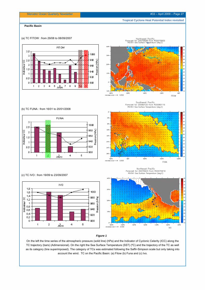
Mercator Ocean Quarterly Newsletter #33 – April 2009 – Page 27
Tropical Cyclone Heat Potential Index revisited
Pacific Basin
(a) TC FITOW : from 29/08 to 08/09/2007
(b) TC FUNA : from 16/01 to 20/01/2008
(c) TC IVO : from 19/09 to 23/09/2007
Figure 1
On the left the time series of the atmospheric pressure (solid line) (hPa) and the Indicator of Cyclonic Celerity (ICC) along the TC trajectory (bars) (Adimensional). On the right the Sea Surface Temperature (SST) (ºC) and the trajectory of the TC as well as its category (line superimposed). The category of TCs was estimated following the Saffir-Simpson scale but only taking into
account the wind. TC on the Pacific Basin: (a) Fitow (b) Funa and (c) Ivo.

Mercator Ocean Quarterly Newsletter #33 – April 2009 – Page 28
Tropical Cyclone Heat Potential Index revisited
The TC FELIX (Figure 2), shows that even when forcing is not able to foreseen the TC the answer of the ICC makes possible to predict the intensity of TC.
TC FELIX: from 01/09 to 04/09/2007
Figure 2
Same as figure 1 but in the Atlantic basin for TC FELIX.
The same analysis is shown for the Indian basin (Figure 3) with similar results to those shown previously for the Pacific and Atlantic basins. These results show the capacity of the ICC once again to predict the digging or filling of a TC.
Indian Basin
(a) TC NARGIS: from 28/04 to 03/05/2008
(b) TC HONDO: from 06/02 to 12/02/2008
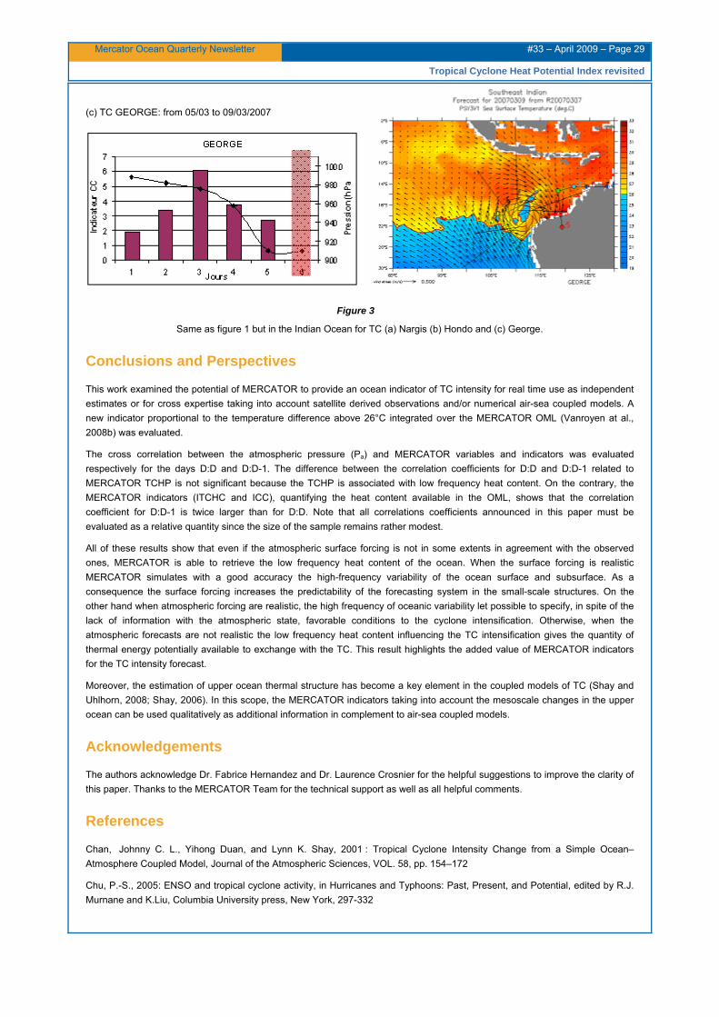
Mercator Ocean Quarterly Newsletter #33 – April 2009 – Page 29
Tropical Cyclone Heat Potential Index revisited
(c) TC GEORGE: from 05/03 to 09/03/2007
Figure 3
Same as figure 1 but in the Indian Ocean for TC (a) Nargis (b) Hondo and (c) George.
Conclusions and Perspectives
This work examined the potential of MERCATOR to provide an ocean indicator of TC intensity for real time use as independent estimates or for cross expertise taking into account satellite derived observations and/or numerical air-sea coupled models. A new indicator proportional to the temperature difference above 26°C integrated over the MERCATOR OML (Vanroyen at al., 2008b) was evaluated.
The cross correlation between the atmospheric pressure (Pa) and MERCATOR variables and indicators was evaluated respectively for the days D:D and D:D-1. The difference between the correlation coefficients for D:D and D:D-1 related to MERCATOR TCHP is not significant because the TCHP is associated with low frequency heat content. On the contrary, the MERCATOR indicators (ITCHC and ICC), quantifying the heat content available in the OML, shows that the correlation coefficient for D:D-1 is twice larger than for D:D. Note that all correlations coefficients announced in this paper must be evaluated as a relative quantity since the size of the sample remains rather modest.
All of these results show that even if the atmospheric surface forcing is not in some extents in agreement with the observed ones, MERCATOR is able to retrieve the low frequency heat content of the ocean. When the surface forcing is realistic MERCATOR simulates with a good accuracy the high-frequency variability of the ocean surface and subsurface. As a consequence the surface forcing increases the predictability of the forecasting system in the small-scale structures. On the other hand when atmospheric forcing are realistic, the high frequency of oceanic variability let possible to specify, in spite of the lack of information with the atmospheric state, favorable conditions to the cyclone intensification. Otherwise, when the atmospheric forecasts are not realistic the low frequency heat content influencing the TC intensification gives the quantity of thermal energy potentially available to exchange with the TC. This result highlights the added value of MERCATOR indicators for the TC intensity forecast.
Moreover, the estimation of upper ocean thermal structure has become a key element in the coupled models of TC (Shay and Uhlhorn, 2008; Shay, 2006). In this scope, the MERCATOR indicators taking into account the mesoscale changes in the upper ocean can be used qualitatively as additional information in complement to air-sea coupled models.
Acknowledgements
The authors acknowledge Dr. Fabrice Hernandez and Dr. Laurence Crosnier for the helpful suggestions to improve the clarity of this paper. Thanks to the MERCATOR Team for the technical support as well as all helpful comments.
References
Chan, Johnny C. L., Yihong Duan, and Lynn K. Shay, 2001 : Tropical Cyclone Intensity Change from a Simple Ocean–Atmosphere Coupled Model, Journal of the Atmospheric Sciences, VOL. 58, pp. 154–172
Chu, P.-S., 2005: ENSO and tropical cyclone activity, in Hurricanes and Typhoons: Past, Present, and Potential, edited by R.J. Murnane and K.Liu, Columbia University press, New York, 297-332

Mercator Ocean Quarterly Newsletter #33 – April 2009 – Page 30
Tropical Cyclone Heat Potential Index revisited
Crosnier, L., M. Drévillon, S. Buarque and F. Soulat, 2008: Three ocean state indices implemented in the Mercator-Ocean operational suite, ICES Journal of Marine Science, 65: 1504–1507.
DeMaria M, and Kaplan J, 1994: Sea surface temperature and the maximum intensity of Atlantic. Tropical cyclones. J Climate 7:1324–1334.
Drévillon, M., Y. Drillet, G. Garric, J.-M. Lellouche, E. Rémy, C. Deval, R. Bourdallé-Badie, B. Tranchant, M. Laborie, N. Ferry, E. Durand, O. Legalloudec, P. Bahurel, E. Greiner, S. Guinehut, M. Benkiran, N. Verbrugge, E. Dombrowsky, C.-E. Testut, L. Nouel and F. Messal, 2006 : The GODAE/Mercator global ocean forecasting system: results, applications and prospects, proceeding of the WMTC conference, London.
Gadgil Sulochana, P V Joseph and N V Joshi, 1984: Ocean-Atmosphereic coupling over monsoonal regions, Nature, 312:141-143.
Goni, Gustavo J. and J.A. Trinanes, 2003: Ocean Thermal Structure Monitoring Could Aid in the Intensity Forecast of Tropical Cyclones, EOS, Transactions American Geophysical Union, VOL. 84, NO. 51, p. 573.
Holland, G.J. 1993: Global Guide to Tropical Cyclone Forecasting, WMO/TC-No. 560, Report No. TCP-31, World Meteorological Organization, Geneva, Switzerland.
Leipper, D. F., 1967: Observed ocean conditions and Hurricane Hilda, Jour. Atmos. Sci., 24:182-196.
Leipper, Dale F and LCDR Douglas Volgneau, 1972: Huricaine Heat Potential of the Gulf of Mexico. Journal of Physical Oceanography, Vol. 2, 218-224.
Madec, G., P. Delecluse, M. Imbard, and C. Lévy, 1998: OPA 8.1 Ocean General Circulation Model reference manual. Note du Pôle de modélisation, Institut Pierre-Simon Laplace, N°11, 91pp.
McBride, J., K. Emanuel, T. Knutson, C. Landsea, G. Holland, H. Willoughby, J. Chan, C.-Y. Lam, J. Heming and J. Kepert, 2006: Statement on Tropical Cyclones and Climate Change by the Membership of the WMO Tropical Meteorology Research Programme Committee, 6th WMO International Workshop on Tropical Cyclones (IWTC-6), San Jose, Costa Rica, November.
Ramos Buarque, S. and V. Landes, 2008: Aptitude du système global de prévision océanique PSY3V2 pour le monitoring des Cyclones tropicaux: un chemin vers le développement d'indicateurs croisés", Ateliers de Modélisation de l’Atmosphère, 22-24 janivier, 10p.
Samson, G, H Giordani, G Caniaux and F Roux, 2008: Analysis of a resonant-like regime in the oceanic mixed layer induced by a moving Hurricane, 24th Conference on Severe Local Storms, 27-31 October 2008, Savannah.
Shay, L. K., 2006: Air-sea interface and oceanic influences, Report for Tropical Cyclone Structure and Structure Change, 6th WMO International Workshop on Tropical Cyclones (IWTC-6), San Jose, Costa Rica, November.
Shay L. K. and E. W. Uhlhorn, 2008: Loop Current Response to Hurricanes Isidore and Lili, Monthly Weather Review, DOI: 10.1175/2007MWR2169.1, Volume 136, Issue 9 (September) pp. 3248–3274.
Sinclair, Mark R., 2002: Extratropical Transition of Southwest Pacific Tropical Cyclones. Part I: Climatology and Mean Structure Changes, Monthly Weather Review, Vol. 130, Issue 3, pp. 590–609.
Vanroyen, C. and C. Agier, 2008a: Réflexion sur le développement d’un indicateur croisé océan-atmosphère pour le monitoring des Cyclones Tropicaux, Projet d’Application des Elèves Techniciens Supérieurs de l’Exploitation de la Météorologie, Rapport N° 1118, Ecole Nationale de la Météorologie (ENM), Toulouse, France.
Vanroyen, C., C. Agier and S. Ramos Buarque, 2008b: Investigation on an oceanic index for monitoring Tropical Cyclones, GODAE Final Symposium, Nice, France, 10-15 november.

Mercator Ocean Quarterly Newsletter #33– April 2009 – Page 31
Assessement of robust Ocean indicators: an example with oceanic predictors for the Sahel precipitations
Assessment of robust Ocean indicators: an example with oceanic predictors for the Sahel precipitations. By Eric Greiner 1, Marie Drévillon 2 1 CLS, Ramonville St Agne, France 2 Mercator Ocean, Ramonville St Agne, France
In this study, we focus on the robustness of the oceanic indicators relatively to the data or model errors, or the data scarcity. In particular, we verify the consistency of an indicator computed from Mercator products (at least eddy permitting ocean forecasting systems) when it was built from coarser resolution time series (for instance ocean reanalysis on a long period back in time or observations networks). We also examine how to optimize an indicator by using several predictors and EOF coefficients time series instead of box averages. This is illustrated all along by the case of the West African Monsoon and more precisely the Sahel precipitations signal, together with Sea Surface Temperature and other oceanic based indicators.
Introduction
Oceanic indicators have been mainly used for climate impact, fish management and biochemistry scenarios. Sea Surface Temperature (SST) is known to force the atmosphere on seasonal to climatic scales. ENSO/El Niño phenomenon has a global impact through the Indo-Pacific SST. Oceanic indicators based on box averages of SSTs have been used for a long time now. Links between the SST and the equatorial rainfalls have been found too. More recently, SST and surface salinity have been shown to impact various fish (Baltic, North Sea, Chili-Peru, etc...). SST also has an impact on the ocean acidification. The SST is thus an excellent proxy to forecast the future of the biogeochemisty. There is clearly an interest and a need to derive oceanic based indicators. But they have to be reliable, and this is still an issue.
Oceanic indicators may have opposite aims. For instance, the RAPID project aims to monitor the long term climate change of meridional heat transport at 27°N in the Atlantic. The Bryden conjecture (Bryden et al., 2005) has shown how important it is to make such a monitoring non sensitive to some “local” climatic pattern (the NAO). Observations from the RAPID mooring array at 26°N show a large sub-annual variability due to changes at the western boundary (Hirschi et al., 2008). Hence, its reliability in terms of climate monitoring is questionable. On the opposite, to forecast the NAO sign one season in advance is an important issue for Europe. The detection of this “local” climatic pattern must not be sensitive to the climate change, or other atmospheric patterns (Blocking, Atlantic Ridge...). Clearly, the sensitivity or robustness of an indicator depends on its objective. In this study, we propose a simple methodology to tackle this problem.
Most oceanic indicators are generally meaningless in themselves. The Gulf Stream transport west of Florida or the maximum of the Atlantic overturning stream function are such indicators. They do not relate directly to human or animal life being. Some indicators are related to climate issues, to some extent. In general, oceanic indicators concerning the ocean heat or its transport are tried to be linked with the land temperature or precipitations. The links between the ocean SST and the land SST have often been demonstrated, in particular regarding the SOI or the NAO index. In this study, we examine a difficult subject, where the primary oceanic indicator (SST) is linked with a secondary land indicator based on another variable than temperature (monsoon rainfalls).
The African Monsoon
In order to illustrate the purpose of this paper, we consider the case of the West African monsoon (WAM). A “monsoon” (from the Arab word mausim meaning season) is an atmospheric phenomenon linked to the annual climate cycle in tropical and sub-tropical regions of the Indian Ocean, southern Asia and Africa. When it occurs, the inter-tropical convergence zone (ITCZ), also known as the “atmospheric equator”, oscillates from south to north, giving precipitations over the Sahel, then from north to south.
Winds converge along the ITCZ. As described for instance on the AMMA project website http://www.amma-international.org/article.php3?id_article=10 , in summer, when the land is very hot, the convection is strong. The wet and cooler air from the equatorial Atlantic replaces this warm dry air. This creates very strong precipitations events through local convective cloud systems.
When the Atlantic SSTs are colder in the Gulf of Guinea (GOG), the sea-land contrast is stronger. It increases the surface winds. The convection is then weaker along the Guinea Coast, and stronger farther north in the Sahel band. On the opposite, if the GOG SSTs are warm, the ITCZ is in its southern position, and the precipitations are more important along the Guinea Coast.

Mercator Ocean Quarterly Newsletter #33– April 2009 – Page 32
Assessement of robust Ocean indicators: an example with oceanic predictors for the Sahel precipitations
Besides the contrast between the Ocean and the landmasses (West Africa), the WAM is influenced by land conditions (albedo, vegetation, soil hydrology conditions).
The Sahel precipitations
The Sahel is the sub-saharian area going from the Atlantic to the Indian Ocean. In this study, we concentrate on the west Sahel, which is more likely to be influenced by the Atlantic.
Satellite Data from GPCP
There are about 20 weather stations in the west Sahel. Not all were regularly sampled during the past 30 years. There are still difficulties to derive a precipitation index concerning this region. This is also difficult because the convective events are strong but localised. Looking at the last 30 years, there was a strong decay in the precipitations from the fifties to the eighties. This had a major impact on the local populations. The last decade is rainier, but the signal seems noisier.
In order to avoid the weather stations data uncertainty, we will use the satellite data from GPCP. We hope this is more adapted when precipitation budget for small regions are under concern. We extract the averages over the Sahel region (west of 10°E, between [5°N-15°N]). The whole signal reveals that precipitations occur mostly but not only during the summer monsoon. When the mean seasonal signal is removed, one sees that the anomalies do not only concern the yearly maximum of precipitation, but also the fluctuations during the wet season. The anomalies during the dry season are not always negligible.
In this study, we will concentrate on the total amount of precipitation during one year, since it determines the amount of available water for those regions (land soil and dams). We use a 7 months box average (about 6 months) and Lee filter (4 points).
The Sahel wet years that can be identified with this filtered GPCP time series (displayed in the following on Figure 3 to 13) are 1988, 1989, 1994, 1998, 1999 and 2003. The dry years are 1983, 1984, 1990, 1993 and 2002.
This confirms that the GPCP data is similar to the annual rainfall from stations. The great advantage is that it is used in the real time Mercator-Ocean global system.
The EOFs of the GPCP precipitations
In this section, we use the satellite precipitations to derive some geographical pattern. The GPCP anomalies are decomposed over land only otherwise the analysis mainly captures the strong variability over the ocean or over Brazil (not shown). In this case the mode 3 presents a good correspondence with the Sahel rainfall. The time evolution of mode 3 is well captured by a 10°-20°N box average. The correlation between the Sahel box average of the precipitations and the mode 3 time amplitude is good (figure 1). However, the decadal change of the eighties is not represented by this mode. It means that the WAM is not uniquely represented by one atmospheric mode.
Figure 1
GPCP precipitations over land: EOF 3 adimensional spatial structure (left panel) and time coefficients (right panel).
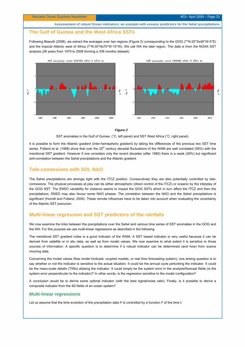
Mercator Ocean Quarterly Newsletter #33– April 2009 – Page 33
Assessement of robust Ocean indicators: an example with oceanic predictors for the Sahel precipitations
The Gulf of Guinea and the West Africa SSTs
Following Biasutti (2008), we extract the averages over two regions (Figure 2) corresponding to the GOG (7°N-20°Sx40°W-5°E) and the tropical Atlantic west of Africa (7°N-30°Nx70°W-10°W). We call WA the later region. The data is from the NOAA SST analysis (28 years from 1979 to 2006 forming a 336 months dataset).
Figure 2
SST anomalies in the Gulf of Guinea (°C, left panel) and SST West Africa (°C, right panel).
It is possible to form the Atlantic gradient (inter-hemispheric gradient) by taking the differences of the previous two SST time series. Folland et al. (1986) show that over the 20th century decadal fluctuations of the WAM are well correlated (59%) with the meridional SST gradient. However if one considers only the recent decades (after 1980) there is a weak (29%) but significant anti-correlation between the Sahel precipitations and the Atlantic gradient.
Tele-connexions with SOI, NAO
The Sahel precipitations are strongly tight with the ITCZ position. Consecutively they are also potentially controlled by tele-connexions. The physical processes at play can be either atmospheric (direct control of the ITCZ) or oceanic by the interplay of the GOG SST. The ENSO variability for instance seems to impact the GOG SSTs which in turn affect the ITCZ and then the precipitations. ENSO may also favour some NAO phases. The correlation between the NAO and the Sahel precipitations is significant (Hurrell and Folland, 2004). These remote influences have to be taken into account when evaluating the uncertainty of the Atlantic SST precursor.
Multi-linear regression and SST predictors of the rainfalls
We now examine the links between the precipitations over the Sahel and various time series of SST anomalies in the GOG and the WA. For this purpose we use multi-linear regressions as described in the following.
The meridional SST gradient index is a good indicator of the WAM. A SST based indicator is very useful because it can be derived from satellite or in situ data, as well as from model values. We now examine to what extent it is sensitive to those sources of information. A specific question is to determine if a robust indicator can be determined (and how) from scarce mooring data.
Concerning the model values (free model hindcast, coupled models, or real time forecasting system), one arising question is to say whether or not the indicator is sensitive to the actual situation. It could be the annual cycle perturbing the indicator. It could be the meso-scale details (TIWs) aliasing the indicator. It could simply be the system error in the analysis/forecast fields (is the system error perpendicular to the indicator)? In other words, is the regression sensitive to the model configuration?
A conclusion would be to derive some optimal indicator (with the best signal/noise ratio). Finally, is it possible to derive a composite indicator from the 4D fields of an ocean system?
Multi-linear regressions
Let us assume that the time evolution of the precipitation data P is controlled by a function F of the time t:

Mercator Ocean Quarterly Newsletter #33– April 2009 – Page 34
Assessement of robust Ocean indicators: an example with oceanic predictors for the Sahel precipitations
P = F(t)
We can approximate it by an Euler discretisation of the time derivative:
P(tn) = P(tn-1) + Δt F(tn-1)
In this example, F(tn) could be some unknown function of the time series of the GOG SSTs. Note that it is not an auto-regressive model since we assume that the precipitations are controlled by something else (a function of the SST for instance).
Let us write the recurrence for this expression, and sum it over n terms:
P(tn) = P(t0) + Δt F(ti-1)
It means that the precipitation data P(tn) at the time are given by some time integral (convolution) of the n last terms of the
unknown function F(tn). Let us assume now that the function depends explicitly on the parameter x, which could be the SST.
Thanks to the Taylor formulae, using the function derivative DF, we can approximate F(x; tn) by its first order approximation near the parameter value a (the average for instance):
F(x; tn) = F(a; tn) + DF(a; tn)(x(tn)−a)
Finally, the precipitation data at a given time are given by a weighted sum (convolution) of the input time series (SST):
P(tn) = P(t0) + ci x(ti)
If we make the additional assumption that the initial condition P(t0) has a negligible impact on the forecast after a long enough time (n>>1), it is possible to rewrite the problem in a set of linear equations for the coefficients ci :
P(tn) = c0 + ci x(ti) + εi for all possible i in the data
The coefficients ci can easily be determined by a least square resolution. The εi are the remaining error between the data and
the fit. The number of terms n tells how many dates are required to predict the data. If the input time series is given monthly and n is 24, then it means that the data memory is 2 years. In this study, we use 6 months running averages of the monthly values, in order to represent the wet-dry seasons budget. Only SSTs values older than 6 months are used to predict the precipitations. We thus introduce the time lag parameter L:
P(tn) = c0 + ci x(ti-L)
In the rest of this study, we will only consider values of L higher than 6 months. Of course, the lag parameter is also an unknown of the estimation. It is determined by a shooting technique.
Link between the Sahel precipitations and the Atlantic SSTs
Here, we search for the best regression between the Sahel precipitations and the WA SST time serie. The SST data is the NOAA analysis. This best regression is search from 1986 and 1997 (the green vertical bars on Figure 3 to 13). We have discarded the older data because of the data uncertainty concerning those dates. The recent dates (1998 to 2007) are kept as independent data for verification. They are not used to determine the regression. The thick black line is the precipitation data. The thin black line is the SST time series, used to fit the data. The thick blue line is the fit to the data. On the lower right of the plot, the time correlation “cor” between the data and the fit is indicated for the dates between 1987 and 2007. It does include the verification data. The “lag” indicates the forecast leading time. For instance, a lag 13 tells us that the fit can be predicted more than a year in advance. The “Nterms” indicates how many terms are used to form the fit. A value of 24 indicates that two years of monthly averages are necessary to form the fit. The “KSs” is the Hanssen and Kuipers score (Hanssen and Kuipers, 1965). It is a score calculated for deterministic forecasts, ranging from zero to one. A 50% value corresponds to the random. Higher values of the score correspond to an improved forecast skill. The KSs score is computed from a contingency table (hit, miss,

Mercator Ocean Quarterly Newsletter #33– April 2009 – Page 35
Assessement of robust Ocean indicators: an example with oceanic predictors for the Sahel precipitations
false alert and nothing). In this study, we arbitrary say that an event occurs when the data is farther from the mean value by more than 2/3 of the standard deviation. On the plot, the orange squares indicate that the fit failed to forecast the data. It can be because the signal is under-estimated (no alert) or over-estimated (false alsert). The green squares indicate that the fit succeed to forecast the event.
If we try to fit the Sahel precipitations with the WA SST, the correlation (13%) is not significant, and the KSs score is less than random (46%). It means that the West Africa SST is not linked with the Sahel precipitations. The Gulf of Guinea SST gives a good fit to the Sahel precipitations (not shown) but the forecast is almost dull (KSs score near 50%). The Meridional SST gradient gives a rather good fit. There is some skill in forecast mode (KSs score=56%). This confirms the works from Biasutti (2008).
Figure 3
Thick black line: Sahel precipitation data from GPCP (mm/day).Thin black line: SST gradient (°C) predictor. Thick blue line : linear regression (fit) of the predictor to the Sahel precipitation data. Orange squares: KS score indicates the predictor fails to predict the event. Green squares: KS score indicate the predictor is successful. See the text for more detailed explanations.
Link between the rainfall and the two model SST predictors from the Atlantic
So far, we have used only one predictor (a single input time series) to fit the precipitations. In the last example, we have used the meridional gradient of SST. A question is whether or not the use of both time series (GOG and WA SSTs) would be useful. A regression can be obtained in the same way, simply by doubling the size of the input series. There are twice more coefficients, and the fit is generally better (Figure 4). The restriction here is that the lag is the same for both series.
Figure 4
Same as figure 3 but with two SST predictors (GOG and WA SST in °C)
It works well for the Sahel in the period 1988-2002, when the NAO signal was strong in the Atlantic. 2004 is a serious false alert. It is possible that an additional signal affects the SSTs after 1998. It could be polluted by the global warming (Atlantic Multi-decadal Oscillation, AMO, [Enfield et al., 2001]). It reveals that box averaged SST indicators could be too sensitive to long term climatic change.

Mercator Ocean Quarterly Newsletter #33– April 2009 – Page 36
Assessement of robust Ocean indicators: an example with oceanic predictors for the Sahel precipitations
EOF decomposition and tele-connexions
Instead of using box averages, we use in this section the time amplitude of the first EOF of the decomposition of observed Tropical Atlantic NOAA SST and model meridional current.
Figure 5
Same as Figure 3 but with the first EOF of Tropical Atlantic SST from NOAA (adimensional) as a predictor (left panel). The spatial structure of the EOF (°C) is displayed on the right panel.
As can be seen on Figure 5, the regression between the Sahel rainfall and the first EOF of SST gives a good fit (the best so far), and a good forecast. The EOF pattern is more optimal than the box average.
Figure 6
Same as Figure 3 but with the first EOF of Tropical Atlantic surface meridional velocity from PSY2G2 reanalysis (adimensional) as a predictor (left panel). The spatial structure of the EOF (m/s) is displayed on the right panel
We also consider the first EOF of the meridional current (from PSY2G2 as described in section 0). The equatorial upwelling described by this EOF (Figure 6) means a cooler SST, which reinforces the WAM. The regression between the precipitation and this EOF gives a good skill before 1999, but it deteriorates afterwards. This could be due to a trend in ERA40 winds (homogenization is necessary), and thus analysed currents. It shows that it is difficult to use variables that are not strongly constrained by the assimilation. Indicators are sensitive to the non-homogeneity of a reanalysis.
Finally, we consider the link with the NAO, as given by the first SST EOF in the North Atlantic (Figure 7). The link is significant before 1999. After that, the forecast of the variability is almost perfect, but there is a negative shift in the predicted values. The removal of a linear trend does not significantly improve the fit (KSs 55%).

Mercator Ocean Quarterly Newsletter #33– April 2009 – Page 37
Assessement of robust Ocean indicators: an example with oceanic predictors for the Sahel precipitations
Figure 7
Same as Figure 3 but with the first EOF of North Atlantic SST from PSY2G2 reanalysis (adimensional) as a predictor (left panel). The spatial structure of the EOF (°C) is displayed on the right panel.
This EOF may be polluted by the global warming (AMO), or some other mode. If one compares with the NCEP NAO index based on sea level pressure, the values are very close. Yet, the regression deduced from this classical index is actually worse as the KS rate is 50% and the correlation only 25% (not shown).
It seems that the Tropical Atlantic and the North Atlantic play an important role in the Sahel precipitations, as suggested in the introduction. We now use the first mode from the ATLG and the NAO to fit the Sahel precipitations, each EOF time series with its own lag (7 and 5 respectively). As shown on Figure 8, the fit and the forecast are good with 50 terms (about 4 years). Note that the fit is excellent when all recent data are used. It suggests that there is a strong potential to monitor and predict 6 months in advance the Sahel precipitations with several ad hoc SST indicators. The Atlantic meridional gradient and the NAO SST tripole are the most influencing parameters so far.
Figure 8
Same as Figure 3 but with the first EOF of SST in the North Atlantic (adimensional) and the first EOF of SST in the tropical Atlantic (adimensional) as predictors. On the left panel recent data are discarded as on Figure 3, and on the right panel recent
data are included in the regression.
Mercator Ocean Quarterly Newsletter #33– April 2009 – Page 38
Assessement of robust Ocean indicators: an example with oceanic predictors for the Sahel precipitations
Sensitivity to the input
We have defined some ocean indicators (box averages or EOF time series) that can be used to monitor and forecast the WAM index. We have seen that the box averages were less performing than the EOF time series. Several other questions arise about the sensitivity to the input:
Is the result different if the observed SSTs are replaced by a forced model or an analysis?
Is the result different if the resolution of the analysis is increased?
Is the result sensitive to analysis uncertainty?
To answer this in the following sections, we will compare the various inputs (time series). The question is then to use the regression derived from the observed data, or to derive a new regression from the new inputs. However, this cannot be achieved with a short hindcast (model with ¼° or 1/12° degree resolution). This sensitivity to the model resolution and cycling will be explored by mixing two reanalysis of different characteristics.
Box averages: satellite and model SSTs
In the following, we will use data from the PSY2G2 1979-2007 reanalysis (Ferry, 2003, 2007). The global ocean model is based on the OPA8.2 code and uses the ORCA2 global ocean configuration. The grid is isotropic (Mercator grid, about 2°x2°cos(latitude) in longitude x latitude) at mid and high latitudes with a refinement in latitude between 5°N / 5°S and a meridional resolution of 0.5°. The model uses a vertical z-coordinate with 31 levels whose first 21 levels are in the top 1,000 metres of the ocean. The thickness of the levels varies from 10 m at the surface (within the first 100 m) to 500 m below the 3,000 m level. Restoring terms (for tracers) towards Levitus et al. (1998) 3D temperature and salinity climatology were added with a time scale of 3 years. The model is forced by the daily surface fluxes coming from the ECMWF ERA40 and operational analyses. The assimilation method is a reduced order Kalman filter using the SEEK formulation. The control vector is composed of the 3D temperature and salinity fileds and the 2D barotropic height. The forecast error covariance is based on the statistics of a collection of 3D ocean state anomalies (typically 3 hundred) and is seasonally variable. In our case, the anomalies are high pass filtered ocean states (Hanning filter, length = 21 days) available over the 1992-2001 time period every 3 day. The observation error covariances chosen for each data set are diagonal matrices accordingly to the method proposed by Fu et al. (1993). The length of the assimilation cycle is 7 days.
The box averages of the SST are almost identical for the satellite data and the PSY2G2 reanalysis (not shown).This is a result of the assimilation and the surface restoring (40W/m2).
The best regression obtained with the satellite is very close to the best regression obtained with the model (not shown). Note that we have not replaced the satellite values by the model ones, but optimized the regression. This sensitivity to the input of a given regression is not studied. This demonstrates that the best regression is not sensitive to the input data. In other words, satellite and model SSTs give almost the same result. This result is also valid for the WA and the GOG.
EOFs: satellite and model SSTs
The EOF decomposition of the PSY2G2 run is almost identical for the satellite data and the reanalysis (not shown).
The best regression for the satellite SST is very close to the best regression for the model SST (Figure 9). Again, the regression based on the EOF decomposition (the EOF 1 meridional gradient) is slightly better than the one based on box averages.
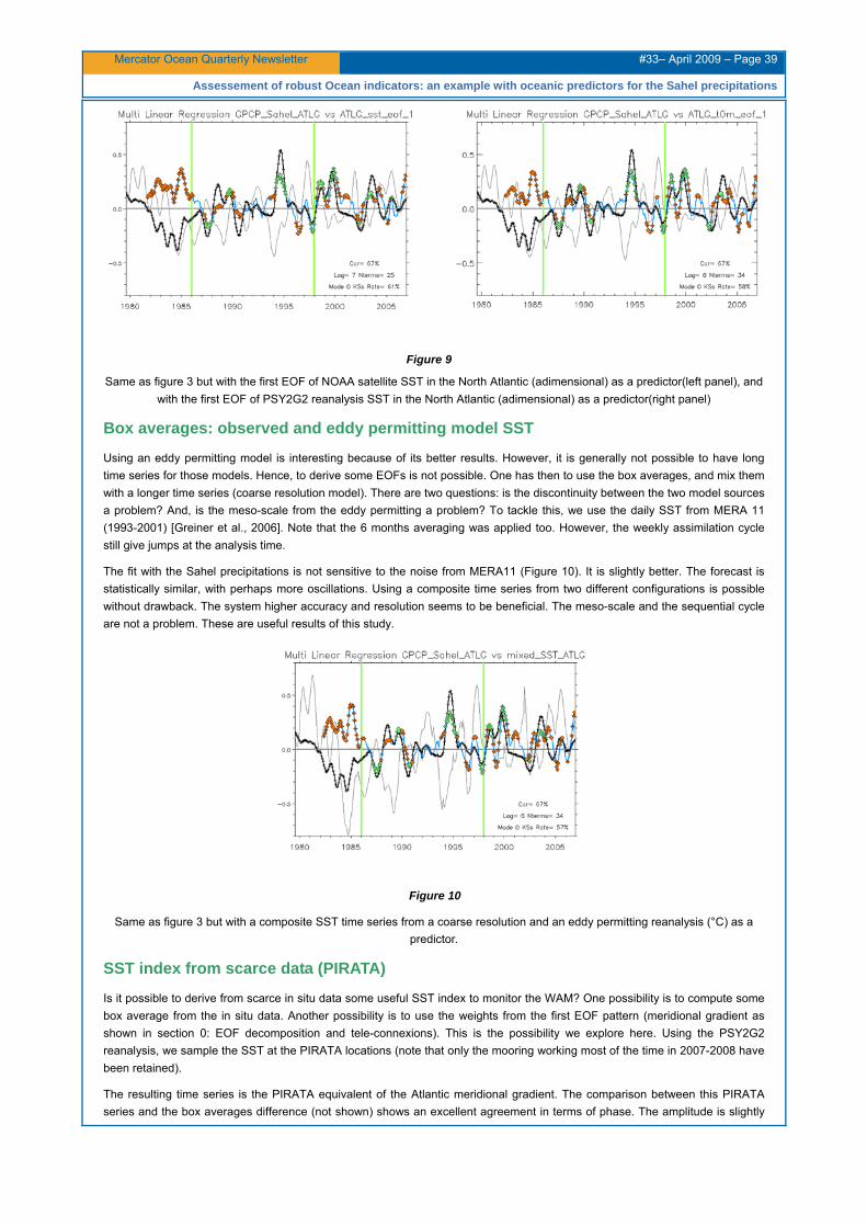
Mercator Ocean Quarterly Newsletter #33– April 2009 – Page 39
Assessement of robust Ocean indicators: an example with oceanic predictors for the Sahel precipitations
Figure 9
Same as figure 3 but with the first EOF of NOAA satellite SST in the North Atlantic (adimensional) as a predictor(left panel), and with the first EOF of PSY2G2 reanalysis SST in the North Atlantic (adimensional) as a predictor(right panel)
Box averages: observed and eddy permitting model SST
Using an eddy permitting model is interesting because of its better results. However, it is generally not possible to have long time series for those models. Hence, to derive some EOFs is not possible. One has then to use the box averages, and mix them with a longer time series (coarse resolution model). There are two questions: is the discontinuity between the two model sources a problem? And, is the meso-scale from the eddy permitting a problem? To tackle this, we use the daily SST from MERA 11 (1993-2001) [Greiner et al., 2006]. Note that the 6 months averaging was applied too. However, the weekly assimilation cycle still give jumps at the analysis time.
The fit with the Sahel precipitations is not sensitive to the noise from MERA11 (Figure 10). It is slightly better. The forecast is statistically similar, with perhaps more oscillations. Using a composite time series from two different configurations is possible without drawback. The system higher accuracy and resolution seems to be beneficial. The meso-scale and the sequential cycle are not a problem. These are useful results of this study.
Figure 10
Same as figure 3 but with a composite SST time series from a coarse resolution and an eddy permitting reanalysis (°C) as a predictor.
SST index from scarce data (PIRATA)
Is it possible to derive from scarce in situ data some useful SST index to monitor the WAM? One possibility is to compute some box average from the in situ data. Another possibility is to use the weights from the first EOF pattern (meridional gradient as shown in section 0: EOF decomposition and tele-connexions). This is the possibility we explore here. Using the PSY2G2 reanalysis, we sample the SST at the PIRATA locations (note that only the mooring working most of the time in 2007-2008 have been retained).
The resulting time series is the PIRATA equivalent of the Atlantic meridional gradient. The comparison between this PIRATA series and the box averages difference (not shown) shows an excellent agreement in terms of phase. The amplitude is slightly

Mercator Ocean Quarterly Newsletter #33– April 2009 – Page 40
Assessement of robust Ocean indicators: an example with oceanic predictors for the Sahel precipitations
under-estimated, and some peaks are different. The regression with the simulated PIRATA (Figure 11) is good. It is similar to the box averages, except the correlation is higher and the forecast skill is lower.
Figure 11
Same as figure 3 but with the first EOF of NOAA satellite SST projected on the PIRATA observations (°C) as a predictor(left panel), and with the Atlantic SST gradient from box averages (°C) as a predictor(right panel).
It means that the indicator based on PIRATA network is nearly as good as based on box averages, when the EOF pattern is used to weight the in situ data. This is very useful to complement the satellite or model based indicators.
Optimal precursor at depth
Lagged correlations between data series (precipitations) and model fields are generally the standard tool to search for some oceanic predictor, or to identify some causal effect. Some examples were given in the beginning. It works when the data and the model series do look the same. It does not work for more complex relations, for instance when the link exists only for some season. Here, we try to reveal some predictor at depth (75m), using as before the EOF decomposition and regression tools. More precisely, we decompose the PSY2G2 temperature and salinity at 75m. The time amplitudes of the EOFs are then regressed against the Sahel precipitations. Generally, the correlation is low (about 30%) and the KSs score is less than random. There are two exceptions. The third EOF in temperature gives a good fit, and a good forecast skill (Figure 12).
Figure 12
Same as figure 3 but with the third EOF of PSY2G2 temperature at 75 m (adimensional) as a predictor(left panel).The spatial structure of the EOF (°C) is displayed on the right panel.
The geographical pattern of the third EOF corresponds to a weakening of the northern trade winds (shallower thermocline north west of the equator) and a reinforcement of the equatorial slope in the GOG probably in response to a strengthening of the local easterly winds. Both are coherent with a northern shift of the ITCZ. This subsurface precursor is potentially very interesting because it is probably less sensitive to air-sea high frequency fluctuations.
The salinity generally gives also poor performances except the third EOF (figure 13).

Mercator Ocean Quarterly Newsletter #33– April 2009 – Page 41
Assessement of robust Ocean indicators: an example with oceanic predictors for the Sahel precipitations
Figure 13
Same as figure 3 but with the third EOF of PSY2G2 salinity at 75 m (adimensional) as a predictor (left panel).The spatial structure of the EOF (psu) is displayed on the right panel.
The geographical pattern of the third EOF corresponds to a mass redistribution from the western off-equatorial band (NECC, SECC) to the equatorial cold tongue (EUC). This is one natural precursor of the Atlantic El Nino. It can legitimately affect the SST and then the WAM. The forecast is not excellent, but it can also be due to the reanalysis accuracy in terms of salinity.
Conclusion
Oceanic indicators have been derived from SST in order to monitor and predict the West African Monsoon. Regional box averages have little skill in this aim. On the contrary, the difference of box averages representing the Atlantic meridional gradient does have a good skill. The range of possible parameters indicates that the previous 6-18 months are the most important to forecast the Sahel precipitations. It confirms that at the first order, the Sahel yearly precipitations are controlled by the SST gradient from the GOG and the West Africa. There is a strong potential to monitor and predict 6 months in advance the Sahel precipitations with several ad hoc SST indicators. The Atlantic meridional gradient and the NAO SST tripole are the most influencing parameters so far. An 83% correlation and a Hit/Miss score of 68% can be obtained.
In theory, the indicator based on a spatial EOF mode will only detect phenomenon span by the time amplitude of the EOF mode. This property is not well obtained for box average indicators, and they are contaminated by various modes. It is even more difficult for network-discrete indicators. In general, we verify that using the EOF pattern is more optimal than the box average. It is difficult to use variables that are not strongly constrained by the assimilation (surface currents, salinity). Indicators are sensitive to the non-homogeneity of a reanalysis. The EOFs still may be polluted by the global warming or multi-decadal scales if the time series is not long enough.
Using a composite time series from two different reanalysis configurations is possible without drawback. The system higher accuracy and resolution seems to be beneficial. The meso-scale and the sequential cycle are not a problem. An indicator based on PIRATA network is nearly as good as based on box averages, when the weights from the ad hoc EOF are used. Finally, some subsurface precursors are potentially very interesting because of a lesser sensitivity to air-sea high frequency fluctuations. These last conclusions support the fact that the MyOcean operational oceanography users (for instance the environmental agencies) will actually benefit from the real time monitoring of these indicators using the MyOcean products. Other indicators will be evaluated with the future GLORYS ocean reanalysis time series, in collaboration with the scientific community. This ensemble of homogeneous time series from global ¼° horizontal resolution experiments, going back in time until 1992 and even earlier for simulations without data assimilation, will be a very good test bench for new indicators.
References
Biasutti, Held, Sobel, and Giannini 2008: SST forcings and Sahel rainfall variability in simulations of the 20th and 21st centuries. Journal of Climate, 21, 3471-3486.
Bryden, H. L., H. R. Longworth and S. A. Cunningham, 2005, Slowing of the Atlantic meridional overturning circulation at 25°N, Nature 438, 655-657, doi:10.1038/nature04385
Enfield, D.B., A.M. Mestas-Nunez, and P.J. Trimble, 2001: The Atlantic Multidecadal Oscillation and its relationship to rainfall and river flows in the continental U.S., Geophys. Res. Lett., 28: 2077-2080.

Mercator Ocean Quarterly Newsletter #33– April 2009 – Page 42
Assessement of robust Ocean indicators: an example with oceanic predictors for the Sahel precipitations
Ferry, N., 2007: Description of Mercator global coarse resolution system PSY2G2, document interne Mercator, 22p, 5 sept.
Ferry, 2003, Définition du prototype Minipog, document interne Mercator n° MOO-ST-424-226-MER, 24p.
Folland, C. K. , T. N. Palmer & D. E. Parker, Sahel rainfall and worldwide sea temperatures, 1901-85, Nature 320, 602 - 607 (17 April 1986); doi:10.1038/320602a0
Fu, L.-L., I. Fukumori and R. N. Miller, 1993. Fitting dynamic models to the Geosat sea level observations in the Tropical Pacific Ocean. Part II: A linear, wind-driven model, JPO, 23, 2162-2181.
Greiner, E., M. Benkiran, E. Blayo, G. Dibarboure, 2006: MERA-11 general scientific paper, 1992-2002 PSY1V2 reanalysis, reference MOO-MR-431-37-MER, 68 pp., Mercator-Ocean, Toulouse, France.
Hanssen A. W., and W. J. A. Kuipers, 1965: On the relationship between the frequency of rain and various meteorological parameters. Meded. Verh., 81, 2\u201315.
Hirschi, J. M., Peter D. Killworth, Jeffrey R. Blundell, David Cromwell, 2008, Sea surface height signals as indicators for oceanic meridional mass transports, Journal of Physical Oceanography, DOI: 10.1175/2008JPO3923.1
Hurrell, J., & C. Folland, 2004, Northwest European High Summer Climate Variability, the West African Monsoon and the Summer North Atlantic Oscillation, C20C WORKSHOP, Trieste.
Levitus S, T P Boyer, M E Conkright, T O'Brien, J Antonov, C Stephens, L Stathoplos, D Johnson, R Gelfeld. NOAA Atlas NESDIS 18, WORLD OCEAN DATABASE 1998: Vol. 1: Introduction, U.S. Govt. Print. Off., Washington, D.C., 346 pp, (1998).

Mercator Ocean Quarterly Newsletter #33 – April 2009 – Page 43
Notebook
0BNotebook
Editorial Board:
Laurence Crosnier
Secretary:
Monique Gasc
Articles:
Estimating Global Ocean indicators from a gridded hydrographic field during 2003-2008
By Karina von Schuckmann, Fabienne Gaillard and Pierre-Yves Le Traon
Intercomparison of environmental Ocean indicators: a complementary step toward scientific expertise and decision making
By Laurence Crosnier, Marie Drévillon, Silvana Ramos Buarque, Jean-Michel Lellouche, Eric Chassignet,
Ashwanth Srinivasan, Ole Martin Smedstad, Sanjay Rattan and Allan Wallcraft
Mediterranean Marine environmental indicators from the Marine Core Service
By Giovanni Coppini, Vladyslav Lyubartsev, Nadia Pinardi, Claudia Fratianni, Marina Tonani, Mario Adani, Paolo Oddo and Srdjan Dobricic, Rosalia Santoleri, Simone Colella and
Gianluca Volpe
Tropical Cyclone Heat Potential Index revisited
By Silvana Ramos Buarque, Claude Vanroyen and Caroline Agier
Assessment of robust Ocean indicators: an example with oceanic predictors for the Sahel precipitations
By Eric Greiner and Marie Drevillon
Contact :
Please send us your comments to the following e-mail address: [email protected] UH
Next issue: July 2009