Mental Accounting and Mobile Banking: Can labelingan M-PESA account increase savings?∗

Preliminary Results - Please Do Not Cite or Circulate

Felipe Dizon† Erick Gong‡ and Kelly Jones §

October 2015

Abstract

Working with a sample of vulnerable women in Kenya, we conduct a field experi-ment involving a savings intervention consisting of a labeled mobile banking (M-PESA)account, savings goal setting, and text message reminders. The effect of the interven-tion on savings is positive but imprecisely estimated. The intervention did lead tostatistically significant increases in savings for those who report having problems sav-ing due to spending on temptation goods. In addition, individuals with temptationconstraints to savings spent less on temptation goods as a result of the intervention.We provide suggestive evidence that the increase in savings for those facing temptationconstraints was most likely due to the labeled M-PESA account. This suggests thatthe labeling of a mobile banking savings account may induce mental accounting andcan relax temptation constraints to savings.

∗The authors received invaluable support from Malin Olero of KidiLuanda Community Programme,Petronilla Odonde of Impact Research and Development Organization, and Alexander Muia, ElizabethKabeu, Sylvia Karanja, and Evans Muga of Safaricom. Special thanks also to Lawrence Juma, Jemima Okal,Matilda Chweya and Joyce Akinyi for excellent management of field work and IPA Kenya for administrativesupport. We thank Tanya Byker, Peter Matthews, John Maluccio, and participants at the MiddleburyEconomics Seminar for useful comments. Research funding was provided by the Hewlett Foundation, IFPRI,Middlebury College, an anonymous donor, and the UC Davis Blum Center. All activities involving humansubjects were approved by IRBs at IFPRI, Middlebury College, UC Davis, and the Maseno University EthicsReview Committee in Kenya. All errors are our own.†PhD Candidate, Agricultural and Resource Economics, University of California- Davis (ffdi-

zon@ucdavis.edu)‡Assistant Professor, Economics Department, Middlebury College (egong@middlebury.edu)§Research Fellow, International Food Policy Research Institute (K.Jones@cgiar.org)

1

1 Introduction

The use of savings programs targeted at the poor in low-income countries is an area ofgrowing focus in both research and policy circles. A number of recent studies have examinedthe various constraints to savings such as transactions costs, social appropriation, and self-control problems.1 On the policy front, influential development organizations such as theBill and Melinda Gates Foundation, have increased emphasis on opening access to savingsproducts for the underbanked.2 Coincidentally, at the same time as interest was growingin savings access for the poor, mobile banking services have become increasingly popular.Mobile banking services are attractive to the poor because they provide safe places to storemoney and have lower transaction fees than formal banks. By far the most popular ofthese services is M-PESA in Kenya, where over 70% of households have adopted it (Suri,Jack, and Stoker, 2012). This paper examines the effect of offering a M-PESA account thatis specifically labeled for savings goals and emergencies on savings behavior of vulnerablewomen in Kisumu, Kenya.

The importance of savings is twofold: it serves as a buffer for unexpected negative shocksand it allows individuals to accumulate small deposits to invest in larger productive assets.Our study is particularly focused on how savings can act as a buffer; insufficient savings canlead individuals to take costly actions during a negative shock. For example, women maysell productive assets or engage in transactional sex (i.e. sex for money) to cover unexpectedmedical expenses. In our context, transactional sex may be particularly costly as the womenin our study reside in Kisumu, Kenya which has some of the highest rates of HIV in EastAfrica (18.7% prevalence).3 Given that negative shocks are common, why don’t the poorsave more? A number of constraints to savings have been proposed; we focus on socialappropriation and self-control problems. Social appropriation is when family and friendshave claims on an individual’s resources and act as a tax on savings.4 Self-control problemsare varied, but the one we focus on in this study is temptation - specifically individualspurchase temptation goods instead of saving surplus funds.

Our study evaluates an intervention designed to alleviate social appropriation and temp-tation constraints to savings. Our sample consists of over 600 vulnerable women in Kisumu,Kenya who all have an existing mobile phone and M-PESA account (“First M-PESA Ac-

1See Karlan, Ratan, and Zinman (2014) for a comprehensive review of the leading constraints to savingsthat the poor in low-income countries face.

2The Bill and Melinda Gates Foundation in 2010 pledged $500 million to expand savings access in thedeveloping world.

3HIV-prevalence figure comes from Kenya AIDS Response Profess Report (2014).4The empirical evidence appears mixed with regards to social appropriation being a binding constraint.

Jakiela and Ozier (2012) find evidence of social claims on investment gains in a lab experiment in the field inKenya, while Brune et al. (2015) find that their commitment savings product did not lead to fewer transfersto relatives nor did publicly releasing savings balances affect any observable behaviors.

1

count”). Women were randomly assigned on an individual basis to either the control orsavings treatment arm. The savings treatment consists of setting up savings goals and open-ing a new “labeled” M-PESA account.5 Women were encouraged to use the labeled M-PESAaccount to save for their goals and to accrue a buffer stock for use in the event of an emer-gency. The funds in the labeled M-PESA account could be withdrawn at any time withoutpenalty. The hypothesis is that the labeled M-PESA account would induce mental account-ing which would help alleviate social appropriation and temptation spending. We follow upwith everyone in the study at midline (3 months) and endline (9 months).

We find that the savings intervention lead to positive but imprecisely estimated increasesin M-PESA balances (First + Labeled M-PESA accounts) and total savings at both midlineand endline.6 To shed light on whether there are binding constraints to savings, we askwomen at baseline whether social appropriation or temptation is preventing them from sav-ing more. We find some evidence that our intervention helps those with social appropriationpressure save more. Our strongest finding is those facing temptation constraints save sig-nificantly more when offered the labeled M-PESA account. Women who face a temptationconstraint save an average of 315 KsH ($3.71) more in their M-PESA accounts and 1116KsH ($13) in liquid savings at endline.7 These estimates are robust when outliers are takeninto account via winsorizing. The savings effects are economically meaningful as well - theincreases amount to over a doubling of M-PESA and liquid savings compared to those withtemptation problems in the control arm. In addition, we show that our intervention reducesspending on two temptation goods (hairdressing and cosmetics) for those who report thattemptation spending is preventing them from saving more.

While our savings treatment is a package of interventions, we provide suggestive evidencethat it is the labeling of the M-PESA account that is driving the results. Given that thefunds in the labeled M-PESA account are fungible (no to minimal withdraw fees), it is mostlikely that the labeling of the account is inducing some form of mental accounting.

Our findings contribute to the growing literature on increasing savings access to thepoor (see Karlan, Ratan, and Zinman (2014) and Table 3 in Prina (2015) for comprehensivereviews).8 Our study is perhaps most motivated by Dupas and Robinson (2013b) which

5Additional elements of the intervention include SMS (Text) reminders of a woman’s savings goals for thefirst 12 weeks of the study. A weekly lottery where everyone in the treatment and control arms was eligiblefor was also conducted during the first 12 weeks of the study. Full details are provided in Section 2.3.

6Total savings is the total of M-PESA balances, other mobile phone balances, money kept under themattress or with family and friends, and bank account balances).

7Liquid savings is the total of M-PESA balances, other mobile phone balances, and money kept underthe mattress or with family and friends,

8There are a number of studies that implement randomized offers to individuals to open formal bankaccounts. Studies have explored whether opening account fees and minimum balances acted as barriers tosavings accounts (Prina (2015); Dupas and Robinson (2013a); Schaner (2013)). Other studies looked atwhether variation in interest rates affect adoption (Karlan and Zinman (2013); Schaner (2013)). Anotherstrand of the savings literature focuses on whether commitment savings products can help the poor save,

2

provided mostly women in rural Kenya various types of savings devices. In two of theintervention arms, a metal box with a lock was provided to deposit savings; in the “safe box”arm the key was given to the individual, while in the “lock box” arm the key was kept by aprogram officer. They study finds that the soft-commitment of the safe box was more effectivethan the hard commitment of the lock box in accumulating savings for preventive healthexpenditures. Our study extends this further by using a mobile banking savings accountas a soft-commitment device. We note two important differences. First, mobile banking ismuch more scalable and provides a high levels of security than a metal lock box (M-PESAwithdraws require both photo identification as well as a personal identification number).9

The second difference is that we are able to make progress on a key constraint that thelabeled account is relaxing: temptation spending. Temptation goods present good-specificdiscount factors that can lead individuals to under-save (Banerjee and Mullainathan, 2010);our findings suggest that simply labeled a widely used savings product might be enough tocurb temptation spending.

Our study was registered with the American Economic Association registry for random-ized control trials (Trial Number: AEARCTR-0000323). We submitted a pre-analysis planafter baseline data was collected (but not yet analyzed), but before the midline data collec-tion commenced. Overall, our study adheres to the pre-specifications of estimating equationsand outcomes quite closely.

2 Study Design

2.1 Financial Services in Kenya and M-PESA

M-PESA, operated by the leading mobile service provider Safaricom, is a highly successfulprivate enterprise which provides clients with branchless banking accessed via mobile phone.Any individual with a national ID card and Safaricom SIM card can set up an M-PESAaccount, allowing her to make deposits, withdrawals and transfers using her mobile handset.M-PESA points are ubiquitous; they are located at nearly every shop and one can be foundopen at nearly any time of day. The district in which this study is set has fewer than 3formal financial institutions per 100,000 population (Kenyan average across all districts is5.3). In contrast, the region has 38 mobile network vendors per 100,000 population.10

especially those with behavioral biases or other-control problems (Ashraf, Karlan, and Yin (2006);Bruneet al. (2015);Dupas and Robinson (2013b); Karlan and Linden (2014)).

9While both the safe box and lock box have a lock, it is conceivable that a thief could simply take themetal box and defeat the lock.

10Authors’ analysis of data from Gaul (2012). Formal institutions are defined as Banks, Micro-financeinstitutions, Mortgage finance institutions, and PostaBanks; excludes cooperatives.

3

2.2 Sample

Our sample consists of 627 vulnerable women in both urban and rural areas in KisumuCounty on the western edge of Kenya. The urban sample consisted of female sex workers(FSWs) and the rural sample consisted of widows, separated or divorced women, or never-married female heads-of-household.11 The women in the rural sample were deemed to beat high-risk of entering into sex work. The sample selection was aimed at examining thelinkages between savings and a risk-coping behavior common in this setting – transactionalsex.

Table 1 provides summary statistics for the full sample as well as the rural and urbansamples. The women in the study have an average age of 28 years and less than half havecompleted primary school. Household size is about 3.5, and this consists primarily of childdependents. Relationship status is somewhat evenly distributed between single, widowed,and divorced/separated, however the rural sample has a higher proportion of widows whilethe urban sample has a higher proportion of single women.

Women in our sample are considerably vulnerable: 66% of the women are categorizedas severely food access insecure based on the Household Food Insecurity Access Scale orHFIAS (Coates, Swindale, and Bilinsky, 2007). Average weekly income is about $19 USD(1648 KsH) which is about 20% less than the average income in Kenya.12 Average incomesand expenditures are higher in the urban sample; this is consistent with the differences inoccupational choice between the two samples. Women in the urban sample are primarilycommercial sex workers and this type of work typically pays a higher premium compared toshop keeping or agriculture.

Women were queried about savings goals, and only 40% reported having one. Of thosewho reported having a savings goal, a majority cited that they were saving for unexpectedexpenses. When women in the study were asked what prevented them from accumulatingsavings, the three most cited responses were: lack of income (90%), spending on temptationgoods (19%) , and pressure to share by family and friends (9%).

Finally, it is important to note that everyone in the sample has an existing M-PESAaccount, which we define as the “First M-PESA account”.

2.3 Intervention and Data Collection

The study involved two local partners that are geographically based. Our urban partneris an NGO that provides health and counseling services to FSWs in Kisumu. The NGO’s

11Women in the rural sample are considered vulnerable because they lacked financial support from a malepartner (i.e. husband or boyfriend).

12GNI per capita in Kenya was $1290 in 2014, which is about $25 per week (World Bank DevelopmentIndicators) .

4

operations include operating “hotspots” which are walk-in centers distributed throughoutKisumu where FSWs can access its services. Our rural partner is a community based organi-zation that targets vulnerable women (i.e. widows, divorced/separated women) and provideseconomic assistance programs. Both partners are well respected in their local communities.

The study has one control arm and two treatment arms and randomization was done on anindividual level. Everyone in the study is grouped into geographic clusters: 12 sub-locationsin the rural sample, and 15 “hotspots” in the urban sample (see Figure 1). We stratified byrural/urban samples and then by geographic cluster. Each cluster was randomly assignedto be a Type I or Type II cluster. Within each cluster, we stratified by age, and then eachindividual was randomly assigned into treatment or control; treatment individuals in TypeI (Type II) clusters were assigned into the Treatment 1 (Treatment 2) arm.

The control group participated in group discussions on the importance of savings thatlasted about one hour. Individuals in the Treatment 1 arm (T1) received the same groupdiscussions as the control arm, plus a one-on-one activity eliciting savings goals, weekly SMSreminders on the savings goals, and a free M-PESA account with zero transaction coststhat we define as the “labeled M-PESA account.” Individuals in the Treatment 2 arm (T2)received everything in the T1 arm and a 5% monthly interest rate on their labeled savingsaccount for the first 12 weeks of the study. We are unable to reject the null that T1 andT2 have the same effect on savings outcomes, and thus we pool the T1 and T2 arms in ouranalysis.

Women in the treatment arm chose savings goals and were told to used the label M-PESAaccount to save for their goals. We also asked each woman in the treatment arm to thinkabout the unexpected expenses that they face and to set aside a specific amount each weekfor emergencies and deposit this into the labeled M-PESA account. The average woman inthe rural (urban) sample set 1.6 (1.3) goals, with a total goal amount of $290 ($600) and anaverage time set to complete one goal at 52 (67) weeks. The average treatment women inthe rural (urban) sample also committed to set aside $1.5 ($0.9) each week for emergencyexpenses. Women were strongly encouraged to only withdraw money from their labeled M-PESA account in the event of an emergency or when they reached their savings goal. Therewere no other restrictions on the labeled M-PESA account, and we thus see this account asa soft commitment device for savings.

The study was carried out in multiple stages (see Figure 2). Stage 1 involved the treat-ment intervention and Stage 2 was a 12 week period where weekly SMS reminders were sentand transaction fees for the labeled M-PESA account were eliminated. Also during Stage 2,everyone in the study (control and treatment arms) was eligible for a weekly lottery. Thelottery was structured to payout 50% of the time, and conditional on winning, an individualwould have a 80% chance of winning one day’s worth of wages, and a 20% chance of winning

5

two day’s worth of wages.13 Each week during Stage 2, a brief survey was conducted tocollect information about shocks and expenditures. After Stage 2 ended, we conducted amidline survey and the weekly lotteries, SMS reminders, and zero transaction costs were alleliminated.

Stage 3 was a 4-month period where monthly SMS reminders were randomly assignedto those in the treatment arm. This was done in order to identify the effects that the SMSreminders have on savings. Once Stage 3 ended, we conducted our endline survey and thenoffered labeled M-PESA accounts to everyone in the control arm.

In addition to using the baseline, midline, and endline survey to construct our dataset, wealso have M-PESA administrative data for all individuals in our study. The administrativedata consists of balances on all of the first M-PESA accounts for the control and treatmentarms as well as balances on the labeled M-PESA account for those in the treatment group.

2.4 Balance of Characteristics between Treatment and Control

Table 2 presents a comparison of baseline statistics between the control and treatment arms.Overall, many characteristics appear similar across the arms. We do note that are signifi-cantly more divorced/separated women in the treatment arm and that while the past week’sincome is not statistically significant at conventional levels, the difference is large.14 Whenthese variables are controlled for, our results are relatively unchanged.

We now turn our attention to savings, and compare the savings balances between thecontrol and treatment arms. Table 3 presents the various savings accounts that individualsin our study have. The first two columns show the percentage of individuals in each armthat have a positive balance in one of the listed accounts (M-PESA, Other Mobile, OwnSavings, Bank Savings). Data for M-PESA is based on administrative data, while all othersavings accounts rely on survey data.15

At baseline, a vast majority in both the control and treatment arm appear to be savingin their M-PESA accounts, and the balances are not trivial - average balances in the control(treatment) arm are about $10 USD ($6.50 USD). Working in our intervention’s favor is thatvery few individuals have another mobile banking account (4%). About 1 in 3 individualshave own savings (i.e. “under the mattress”). Fewer individuals are utilizing formal bankaccounts as a means to save. We also look at illiquid savings in the form of ROSCAS and

13Given the differences in income between the rural and urban sample (see Table 1), the payout for therural sample was 250 KsH (1 day) and 500 KsH (2day) and for the urban sample it was 500 KsH (1-day)and 1000 KsH (2-day).

14Our pre-analysis plan specified that religion would be a baseline characteristics that we would checkbetween the control and treatment arms. At the time of this draft, we do not have data on an individual’sreligion, but plan to incorporate this in future drafts.

15We compare the administrative M-PESA data to the self-reported data and find that on average, self-reported data underestimates actual administrative balances, but there appears to be no differential under-reporting between the treatment and control arms.

6

livestock. Both types of savings appear popular, with a majority participating in a ROSCAand holding livestock. However, we note that calculating present values of assets held inROSCAs and livestock is difficult and measures are very noisy. We therefore do not focuson these measures in our analysis.

Our savings outcomes simply aggregate the individual accounts. M-PESA savings issimply the amounts in all M-PESA accounts, while the other savings outcomes are definedas follows:

• Mobile Savings = M-PESA Savings + Other Mobile Savings

• Liquid Savings =M-PESA Savings + Other Mobile Savings + Own Savings

• Total Savings = M-PESA Savings + Other Mobile Savings + Own Savings + BankSavings

Overall, many of the savings measures at baseline appear to be higher in the control arm,although none of these differences is statistically significant at conventional levels. Giventhese differences, we control for baseline savings measures in our analysis.

2.5 Treatment Take Up

A major concern regarding savings interventions targeted at the poor are the low rates ofuptake and usage (see Prina (2015) ). Uptake of the labeled M-PESA account is particularhigh for our intervention (~98%) which we attribute to the low time and travel costs of ourintervention (individuals in the treatment arms were already participating in a group savingsdiscussion when offered the intervention). We present usage statistics in Table 4.

The first two columns present data on the M-PESA accounts that both the control andtreatment groups had before the study. Usage is measured for both Midline and Endlineand we follow common usage definitions in the literature. The third and sixth columns showusage activity in the Labeled M-PESA account. Using 1 deposit in the period as a measureof usage, the Labeled M-PESA account was used by 58% of those offered the account anddips down to 42% by endline. These usage patterns are similar to other savings interventions.For example, after one year, active usage of a formal bank account in Chile was 39% (Kastand Pomeranz, 2014), of a formal bank account in Nepal 80% (Prina, 2015), and of a simplelockbox in western Kenya 71% (Dupas and Robinson, 2013b).16 Two studies that are similarto ours are both conducted in Kenya and offered formal bank savings accounts: Dupas and

16Active usage is defined differently in each of these studies. Kast and Pomeranz (2014) define activeusage as depositing more than the minimum account deposit, Prina (2015) defines active usage as makingat least 2 deposits in one year, and Dupas and Robinson (2013b) define usage as having a non-zero amountin a lockbox.

7

Robinson (2013a) offered savings accounts to entrepreneurs and document usage of 41%,while Schaner (2013) offered savings accounts to couples and finds usage rates of 22%.

One thing that is interesting to note is the deposit and withdraw activity of the LabeledM-PESA account appears similar. At midline (endline), users of the Labeled M-PESAaccount had an average of 5.1 (7.4) deposits and 3.0 (6.8) withdraws. Total and averageamounts deposited and withdrawn are relatively similar as well. This type of savings activityis more consistent with the Labeled M-PESA account being used as a buffer for shocks asopposed to accumulating savings over time to make large investments.17

Figure 3 shows average daily balances of the Labeled M-PESA account over time. Thedaily mean balance was sharply growing in the beginning of the intense intervention period,and it peaked right before the end of the intense intervention period. In June 2014, meanbalance was 792 KsHs ($9.31) for those that ever used the account. Even after transactionfees were reinstated and interest rates removed from the Labeled M-PESA account, usersstill kept positive balances in this account. About nine months after the initial intervention,average balance was 383 KsHs ($4.50).

3 Effects of Intervention on Savings

3.1 Effects of Intervention on Savings

We now examine the effects that the intervention had on savings outcomes. Figure (4)compares two savings outcomes (M-PESA balances and Total Savings Balances) between thetreatment and control arms. For both M-PESA savings and Total Savings, the treatmentarm starts off with lower balances at baseline - we thus will control for baseline savingsbalances in our formal estimations. For M-PESA savings, we see that both the treatmentand control arms increase savings at midline, but the increase in the treatment arm is morepronounced. We also see declines in M-PESA savings for both arms, but the decrease for thetreatment arm is at a lower rate. In fact, at endline, M-PESA balances are higher for thetreatment arm compared to baseline savings - the same cannot be said for the control arm.A similar pattern is found with Total Savings as well; a relatively large increase in TotalSavings at midline for the treatment arm and then a relatively lower decline by endline. Wenow turn to a formal estimation of the effects of the intervention on savings.

We use the following specification

Savingsi = α + β1Ti ++β2Agei + β3Baseline Savingsi + λj + εi (3.1)17Savings activity that is consistent with the large investment scenario would involve a high number of

small deposits and one or two large withdrawals.

8

where Savingsi is a savings outcome for individual i, Ti is an indicator that the individualwas assigned to the treatment arm, Agei is baseline age, Baseline Savingsi is the baselinesavings outcome, λj are geographic cluster fixed effects, and εi is an individual error term.Both Agei and λj are variables used for stratification, and thus Ti is randomly assignedconditional on these covariates.18 Our estimate of β1 is an intent to treat (ITT) effect.

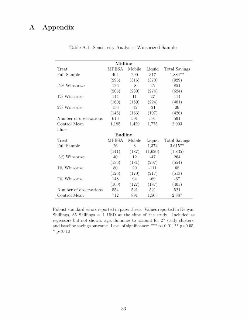
Our first set of results are presented in Table 5. At both midline and endline, all of thepoint estimates are positive, but only the estimate for Total Savings is statistically significantat the 5% level. Given that the variation in Total Savings outcome is large and that reportedbank balances might be noisy, we do sensitivity analysis for these estimates. We winsorizethe savings outcomes at the .5%, 1%, and 2% levels and find that the ITT estimate on totalsavings while still positive is no longer statistically significant (see Appendix Table A.1).Given the imprecision of these estimates, we are unable to infer that the intervention leadto increases in savings.

When women in our study were asked at baseline what constraints they faced with regardsto saving, the leading response was a lack of income (see Tables 1 and 3). We attempt torelieve this constraint by conducting weekly lotteries that give women a 50/50 chance ofa payout worth 1 or 2 days wages. To estimate the effects that lottery winnings have onsavings, we modify equation 3.1 as follows:

Savingsi = α + β1Ti + β2Agei + β3Baseline Savingsi

+β4LotteryTotali + β5(Ti × LotteryTotali) + λj + εi (3.2)

where LotteryTotali is the total lottery winnings for individual i . Mean lottery winningsis 2,701 KsH ($31 USD) ,which represents over a week’s worth of income in both the ruraland urban samples. Table 6 presents the results. We find that total lottery winnings has nostatistically significant effect on any of our savings outcomes. In addition, there appears tobe no differential effect of lottery winnings for those in the treatment arm. It is importantto note that everyone in the study received at least one lottery payoff, and so the pointestimates for Treat are not meaningful. We report ITT estimates at mean lottery winningsin the last row. The lottery results are consistent with the notion that the poor have incomethat they can save and that this is not a binding constraint for savings (Banerjee and Duflo(2007)).

18Baseline Savingsi was not pre-specified as a control in the PAP. The PAP however did specify thatbaseline characteristics that were either imbalanced at baseline or predictive of the outcome would be usedas controls. While we cannot reject the null that the control and treatment have the same savings outcomesat baseline at conventional levels of statistical significance (see Table 3), the differences are large enough inmagnitude to warrant inclusion as a control. Baseline savings are also highly predictive of our savings atboth midline and endline. The inclusion of a baseline savings outcome is also similar to specifications inPrina (2015) who examines the impact of randomized offers of formal bank accounts on savings.

9

We now focus our analysis at heterogenous treatment effects.

3.2 Constraints to Savings (Heterogenous Treatment Effects)

Our intervention was aimed at relaxing social appropriation and self-control/temptationconstraints via the use of the labeled M-PESA account to induce mental accounting. To testwhether our intervention relieved these constraints we estimate the following:

Savingsi = α + β1Ti + β2Agei + β3Baseline Savingsi

+β4Constrainti + β5(Ti × Constrainti) + λj + εi (3.3)

where Contrainti is a baseline measure of either social appropriation or self-control beinga constraint to savings. If our intervention relaxes either of these constraints, we expect thatβ1 + β5 > 0 (treatment effect for those facing the constraint). Equation 3.3 was specified inour analysis plan as were the two constraints (social appropriation and self-control).19

3.2.1 Social Appropriation

We first examine the effects that the savings intervention has on those facing a social appro-priation constraint. At baseline, individuals were asked if they would like to save more, andif they said “yes”, what was preventing them from saving more. Women who stated “Friendsand family ask to share” as a primary constraint are coded as having social appropriationconstraints. In our sample, a relatively small proportion report this as a problem (~9% seeTable 2). We present results for our analysis of social appropriation in Table 7. There is apositive and statistically significant effect for M-PESA savings at both midline and endline(Table 7), and these estimates are stable when outliers are taken into account (AppendixTable A.2). The effect on liquid and total savings are imprecisely estimated; while thepoint estimates for liquid savings are relatively stable, the estimates for total savings is verysensitive to outliers.

One possible explanation for why we see stronger treatment effects on M-PESA is thatit is substantially easier to transfer funds to family and friends using M-PESA. Jack andSuri (2014) document that the predominant use of M-PESA has been for interpersonalremittances. Funds in an M-PESA account maybe subject to greater social pressure to

19Our specific measure of social appropriation uses the pre-specified variable in our pre-analysis plan. Ourspecific measure of self-control (temptation) was not pre-specified. It however follows the same variable thatsocial appropriation comes from which is the answer to the question at baseline “What is preventing you fromsaving more?. The three leading responses are lack of income, temptation spending, and social appropriation(see Table 2).

10

share; the provision of a 2nd M-PESA account that has a specific purpose may ease some ofthis pressure.

Overall, while it appears that the treatment lead to increases in M-PESA savings, itseffects on other savings outcomes is unclear.

3.2.2 Temptation

We now turn to spending on temptation goods as a constraint to savings. Similar to our socialappropriation measure, women at baseline who stated that “spending on temptation goods”was preventing them from saving are coded as having temptation constraints to savings.About 19% of the sample report this as a problem (Table 1). We estimate equation 3.3where Constrainti is equal to one if a woman reports temptation goods being a constraintto savings. Table 8 presents the results.

We do see evidence that the intervention has a positive effect on savings for those withtemptation constraints. Both midline and endline estimates for β2 + β5 are positive for allsavings measures and, with the exception of liquid savings, statistically significant at the10% level or better. These estimates are robust to winsorizing and the estimate for liquidsavings becomes statistically significant when accounting for outliers in this way (Table 9).These estimates are also economically meaningful. Using the 1% winsorized estimates (Table9), the treatment led to over a doubling of M-PESA balances at both midline and endline.The 630 KsH ($7.41) increase in midline M-PESA balances represents about 38% of weeklyreported income.

It is possible that the increase in savings that we see for those with temptation constraintsmay be crowding out other forms of savings. We explore this by estimating treatmenteffects for those with temptation constraints on specific savings accounts and methods (Table10). The first three columns (1st M-PESA Account, Own Savings, and Bank Savings)are components of the main savings outcomes, while the last two columns (ROSCA andLivestock) take into account more illiquid forms of savings. If the labeled M-PESA accountis crowding out other forms of savings, we expect to see lower savings balances in these otheraccounts. Both at midline and endline, we see no evidence for this; in fact, we actuallysee increases in savings balances for some of these accounts. Overall, this suggests that theincrease we see in our main savings outcomes and not a result of substitution away fromother forms of savings.

Finally, if funds in the labeled M-PESA account was mentally earmarked and protectedfrom temptation spending, we should also see reductions in temptation expenditures. Usingour high-frequency weekly surveys, we ask about spending on hairdressing and cosmetics -two expenditures that women in our focus groups mentioned as temptation items. Aggregat-ing the 12-weekly surveys gives us the total amount spent on these two temptation goods.

11

For those with temptation constraints, we find that the intervention led to a reduction intemptation spending (Table 11). The reduction we see in temptation spending (-250 Ksh)represents about 40% of the increase we see in M-PESA savings at midline (Table 8). In ad-dition, we see that the share of food expenditures spent on temptation goods is also reducedby about 2 percentage points.

3.3 Was it the labeled M-PESA account?

Our savings intervention involved more than a labeled M-PESA account, it also includedestablishing savings goals and sent weekly SMS reminders of these goals during the first 12weeks of the study. We provide suggestive evidence that neither of these two interventions(goal setting and SMS reminders) had any substantial effect on savings.

For SMS reminders, we did randomize who would receive them in the treatment armbetween midline and endline. After the midline survey, we randomly chose half of theindividuals in the treatment arm to continue to receive SMS reminders - however thesereminders were now issued on a monthly basis. We estimate the following:

Savingsi = α + β1SMSi ++β2Agei + β3Baseline Savingsi + λj + εi (3.4)

where β1 is the effect of receiving SMS reminders on savings. We find that the the SMSreminders might have had slight positive effect on M-PESA, Mobile, and Liquid Savings,although the estimates are not statistically significant (Table 12). These results are relativelysimilar to those found by Karlan et al. (2014) who find that monthly text messages and lettersabout savings goals increased savings by 6%. Using the 1% winsorized sample, we see thatat endline, liquid savings increased by a statistically significant 1116 Ksh for those withtemptation constraints (Table 9), while the SMS reminders increased savings by 140 Ksh(Table 12) and this estimate is not statistically significant. This suggests that even if SMSreminders had an effect on savings, it is relatively small component of the treatment effect.

With regards to setting savings goals, we note that many of the savings goals establishedinvolved very large amounts (Table 13). For example, the most common savings goal waseducational expenses and the average goal amount was 22,437 KsH. If the goals acted asa commitment device then we would expect the amounts withdrawn from the labeled M-PESA account to be similar to the goals. However, the average amounts withdrawn from thelabeled M-PESA account (1021 Ksh and 1207 KsH at midline and endline respectively) aremuch smaller than the average amounts for any of the savings goals. In fact, the withdrawnamounts are much closer to the amounts set aside weekly for emergency (103 Ksh) whichamounts to 1236 Ksh over the first 12 weeks of the study. While we do not have data onwhat the withdrawals were used for in the labeled M-PESA account, the activity suggeststhat the account was used for emergency expenses as opposed to being used for the reported

12

savings goals.Finally, we survey women in the treatment arm about their experiences with the labeled

M-PESA account. We find that a majority report that the labeled M-PESA account helpedthem save more, and the top reasons given were that it minimized temptation spendingand restricted access to funds (Table 14). Recall that at midline, there were no withdrawalor transfer fees on the labeled account and the funds were very easy to access. The userresponses suggest that some form of mental accounting was being used to restrict access tobalances in the labeled account.

4 Conclusion

We find that providing a labeled M-PESA account without any formal withdrawal restrictionswas able to increase savings. While the results for the full sample are not precisely estimated,the results for those who faced a temptation constraint are statistically significant. We alsonote that people tend to make small withdraws from their labeled M-PESA account; thisactivity is more consistent with using the funds as a buffer for shocks instead of making largepurchases. Future work will examine whether those who see increases in savings as a resultof the intervention are able to better cope with shocks.

13

References

Ashraf, N., D. Karlan, and W. Yin. 2006. “Tying Odysseus to the Mast: Evidence from aCommitment Savings Product in the Philippines.” The Quarterly Journal of Economics121:pp. 635–672.

Banerjee, A., and S. Mullainathan. 2010. “The shape of temptation: Implications for theeconomic lives of the poor.”

Banerjee, A.V., and E. Duflo. 2007. “The economic lives of the poor.” The journal of economicperspectives: a journal of the American Economic Association 21:141.

Brune, L., X. Giné, J. Goldberg, and D. Yang. 2015. “Facilitating Savings for Agriculture:Field Experimental Evidence from Malawi.”

Coates, J., A. Swindale, and P. Bilinsky. 2007. “Household Food Insecurity Access Scale(HFIAS) for measurement of food access: Indicator Guide (v.3).” Food and NutritionTechnical Assistance Project (FANTA)/Academy for Educational Development.

Council, N.A.C. 2014. “Kenya AIDS Response Progress Report.” Kenyan Government , pp. .

Dupas, P., and J. Robinson. 2013a. “Savings Constraints and Microenterprise Development:Evidence from a Field Experiment in Kenya.” American Economic Journal: Applied Eco-nomics 5:163–192.

—. 2013b. “Why Don’t the Poor Save More? Evidence from Health Savings Experiments.”American Economic Review 103:1138–1171.

Jack, W., and T. Suri. 2014. “Risk Sharing and Transactions Costs: Evidence from Kenya’sMobile Money Revolution.” The American Economic Review 104:pp. 183–223.

Jakiela, P., and O. Ozier. 2012. “Does Africa need a rotten Kin Theorem? experimentalevidence from village economies.” Policy Research Working Paper Series No. 6085, TheWorld Bank, Jun.

Karlan, D., and L.L. Linden. 2014. “Loose Knots: Strong versus Weak Commitments to Savefor Education in Uganda.” Working paper, National Bureau of Economic Research.

Karlan, D., M. McConnell, S. Mullainathan, and J. Zinman. 2014. “Getting to the top ofmind: How reminders increase saving.” Working paper, Management Science.

Karlan, D., A.L. Ratan, and J. Zinman. 2014. “Savings by and for the Poor: A ResearchReview and Agenda.” Review of Income and Wealth 60:36–78.

14

Karlan, D., and J. Zinman. 2013. “Price and Control elasticities of Demand for Savings.”Working paper.

Kast, F., and D. Pomeranz. 2014. “Saving More to Borrow Less: Experimental Evidencefrom Access to Formal Savings Accounts in Chile.” Working paper, National Bureau ofEconomic Research.

Prina, S. 2015. “Banking the poor via savings accounts: Evidence from a field experiment.”Journal of Development Economics 115:16–31.

Schaner, S. 2013. “the persistent power of behavioral change: Long-run impacts of temporarysavings subsidies for the poor.” Documento de trabajo. Dartmouth College: Hanover, NH ,pp. .

Suri, T., W. Jack, and T.M. Stoker. 2012. “Documenting the birth of a financial economy.”Proceedings of the National Academy of Sciences 109:10257–10262.

15

Figures

Figure 1: Sample Structure

16

Figure2:

Stud

yTim

eline

17

Figure 3: Labeled M-PESA Account: Balances Over Time

18

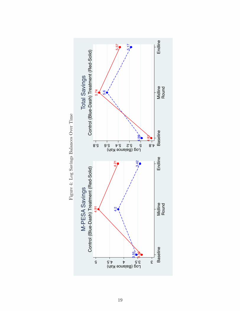
Figure4:

LogSa

ving

sBalan

cesOverTim

e

3.55

4.2

3.42

3.36

4.91

4.21

33.544.55Log (Balance Ksh) Ba

selin

eM

idlin

eEn

dlin

eR

ound

Con

trol (

Blue

-Das

h) T

reat

men

t (R

ed-S

olid

)M

-PES

A Sa

ving

s

4.98

5.6

5.17

4.81

5.74

5.37

4.855.25.45.65.8Log (Balance Ksh) Ba

selin

eM

idlin

eEn

dlin

eR

ound

Con

trol (

Blue

-Das

h) T

reat

men

t (R

ed-S

olid

)To

tal S

avin

gs

19

Tables

Table 1: Baseline Descriptive Statistics

Full Rural UrbanSample (Kadibo) (Kisumu)

DemographicsAge 28.55 27.18 29.95HH Size 3.52 4.20 2.84Single 0.27 0.15 0.39Widowed 0.37 0.56 0.17Divorced/Separated 0.33 0.29 0.37Education: More than Primary Sch 0.39 0.32 0.46Income and ExpensesIncome in past 7 days 1,648 1,441 1,858Primary Income Source: Sex Work 0.43 0.00 0.86Primary Income Source: Shop Keeper/Trading 0.42 0.47 0.36Primary Income Source: Agriculture 0.19 0.37 0.01Spending on temptation goods in past 7 days 408 207 612Spending on non-food expenses in past 30 days 1,386 816 1,966Severe Food Insecurity: HFIAS Scale 0.66 0.73 0.59Food Insecurity: Insufficient Intake 0.85 0.91 0.79Savings Goals and ConstraintsHave Savings Goal 0.40 0.21 0.59Savings Goal: Unexpected Expense 0.55 0.42 0.60Savings Goal: Education 0.16 0.10 0.22Savings Goal: Business 0.08 0.12 0.07Constraint: Income 0.90 0.95 0.85Constraint: Temptation Goods 0.19 0.15 0.23Constraint: Social Appropriation 0.09 0.07 0.11Observations 627 316 311*Temptation goods include jewelry, perfume, cosmetics, clothing, hairdressing, snacks, air-time, meals outside the home, cigarettes, alcohol and recreational drugs. Other non-foodexpenses include car battery, wedding and social events, funeral, health, expenses, fam-ily planning, electronics, household assets and home improvement. Values are reported inKenyan Shillings, 85 Shillings = 1 USD at the time of the study.

20

Table 2: Baseline Balance

Control Treat p-valuemean mean differences

DemographicsAge 28.70 28.39 0.50HH Size 3.55 3.49 0.69Single 0.28 0.26 0.59Widowed 0.38 0.35 0.36Divorced/Separated 0.29 0.37 0.04Education: More than Primary Sch 0.40 0.37 0.43Income and ExpensesIncome in past 7 days 2,122 1,143 0.12Primary Income Source: Sex Work 0.44 0.41 0.58Primary Income Source: Shop Keeper/Trading 0.43 0.40 0.37Primary Income Source: Agriculture 0.19 0.19 0.97Spending on temptation goods in past 7 days 405 410 0.95Spending on non-food expenses in past 30 days 1,554 1,209 0.10Food Insecurity: Anxious Past Month 0.76 0.77 0.89Food Insecurity: Insufficient Intake 0.84 0.86 0.49Savings Goals and ConstraintsHave Savings Goal 0.41 0.39 0.60Savings Goal: Unexpected Expense 0.59 0.50 0.15Savings Goal: Education 0.16 0.16 0.82Savings Goal: Business 0.10 0.06 0.26Constraint: Income 0.90 0.90 0.80Constraint: Temptation Goods 0.21 0.17 0.25Constraint: Social Appropriation 0.09 0.09 0.92

Observations 323 304*Temptation goods include jewelry, perfume, cosmetics, clothing, hairdressing, snacks, air-time, meals outside the home, cigarettes, alcohol and recreational drugs. Other non-foodexpenses include car battery, wedding and social events, funeral, health, expenses, fam-ily planning, electronics, household assets and home improvement. Values are reported inKenyan Shillings, 85 Shillings = 1 USD at the time of the study.

21

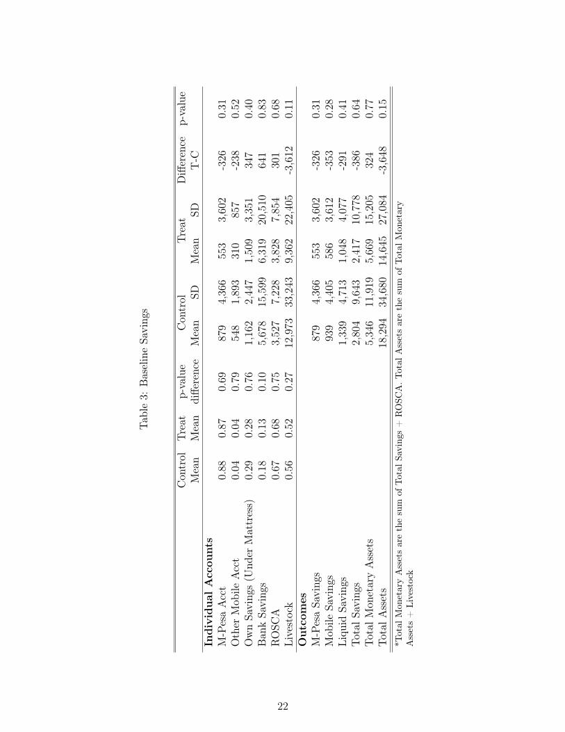
Table3:

BaselineSa

ving

s

Con

trol

Treat

p-value

Con

trol

Treat

Difference

p-value

Mean

Mean

diffe

rence

Mean

SDMean

SDT-C

Indiv

idual

Acc

ount

sM-PesaAcct

0.88

0.87

0.69

879

4,36

655

33,60

2-326

0.31

Other

Mob

ileAcct

0.04

0.04

0.79

548

1,89

331

085

7-238

0.52

OwnSa

ving

s(U

nder

Mattress)

0.29

0.28

0.76

1,16

22,44

71,50

93,35

134

70.40

Ban

kSa

ving

s0.18

0.13

0.10

5,67

815

,599

6,31

920

,510

641

0.83

ROSC

A0.67

0.68

0.75

3,52

77,22

83,82

87,85

430

10.68

Livestock

0.56

0.52

0.27

12,973

33,243

9,36

222

,405

-3,612

0.11

Outc

omes

M-PesaSa

ving

s87

94,36

655

33,60

2-326

0.31

Mob

ileSa

ving

s93

94,40

558

63,61

2-353

0.28

Liqu

idSa

ving

s1,33

94,71

31,04

84,07

7-291

0.41

TotalS

avings

2,80

49,64

32,41

710

,778

-386

0.64

TotalM

onetaryAssets

5,34

611

,919

5,66

915

,205

324

0.77

TotalA

ssets

18,294

34,680

14,645

27,084

-3,648

0.15

*Total

Mon

etaryAssetsarethesum

ofTotal

Saving

s+

ROSC

A.T

otal

Assetsarethesum

ofTotal

Mon

etary

Assets+

Livestock

22

Table 4: M-PESA Usage

Midline EndlineLabeled Labeled

M-PESA M-PESA M-PESA M-PESAControl Treat Treat Only Control Treat Treat OnlyMean Mean

Usage (1 deposit) 0.93 0.93 0.58 0.93 0.89 0.42Usage (2 deposits) 0.86 0.86 0.45 0.86 0.85 0.27Usage (Positive Balance) 0.92 0.85 0.57 0.83 0.84 0.56Balance 862 817 792 675 560 383

Number of Deposits 9.0 8.6 5.1 14.1 13.0 7.4Total Amt Deposited 16,961 12,966 3,968 28,532 23,120 12,088Avg Deposit Amt 1,515 1,265 684 1,731 1,370 1,252

Number of Withdraws 10.7 11.2 3.0 12.3 11.6 6.8Total Amt Withdrawn 17,746 14,168 3,341 24,974 20,016 11,363Avg Withdrawn Amt 1,456 1,150 1,021 1,534 1,344 1,207

23

Table 5: ITT Results

MidlineMPESA Mobile Liquid Total

Savings SavingsTreat 404 290 317 1,884**

(295) (316) (370) (929)Number of observations 616 591 591 591Control Mean 1,185 1,429 1,775 2,903

EndlineMPESA Mobile Liquid Total

Savings SavingsTreat 26 8 1,374 3,615**

(141) (187) (1,620) (1,835)Number of observations 554 521 521 521Control Mean 712 891 1,565 2,887

Robust standard errors reported in parenthesis. Values reported in KenyanShillings, 85 Shillings = 1 USD at the time of the study. Included asregressors but not shown: age, dummies to account for 27 study clusters,and baseline savings outcome. Level of significance: *** p<0.01, ** p<0.05,* p<0.10

24

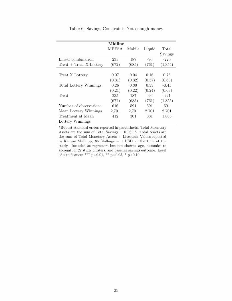
Table 6: Savings Constraint: Not enough money

MidlineMPESA Mobile Liquid Total

SavingsLinear combination 235 187 -96 -220Treat + Treat X Lottery (672) (685) (761) (1,354)

Treat X Lottery 0.07 0.04 0.16 0.78(0.31) (0.32) (0.37) (0.60)

Total Lottery Winnings 0.26 0.30 0.33 -0.41(0.21) (0.22) (0.24) (0.63)

Treat 235 187 -96 -221(672) (685) (761) (1,355)

Number of observations 616 591 591 591Mean Lottery Winnings 2,701 2,701 2,701 2,701Treatment at Mean 412 301 331 1,885Lottery Winnings*Robust standard errors reported in parenthesis. Total MonetaryAssets are the sum of Total Savings + ROSCA. Total Assets arethe sum of Total Monetary Assets + Livestock Values reportedin Kenyan Shillings, 85 Shillings = 1 USD at the time of thestudy. Included as regressors but not shown: age, dummies toaccount for 27 study clusters, and baseline savings outcome. Levelof significance: *** p<0.01, ** p<0.05, * p<0.10

25

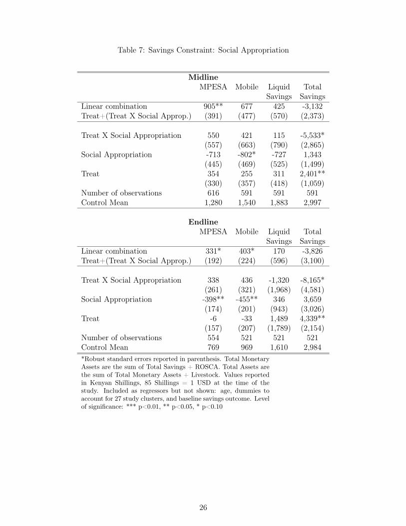
Table 7: Savings Constraint: Social Appropriation

MidlineMPESA Mobile Liquid Total

Savings SavingsLinear combination 905** 677 425 -3,132Treat+(Treat X Social Approp.) (391) (477) (570) (2,373)

Treat X Social Appropriation 550 421 115 -5,533*(557) (663) (790) (2,865)

Social Appropriation -713 -802* -727 1,343(445) (469) (525) (1,499)

Treat 354 255 311 2,401**(330) (357) (418) (1,059)

Number of observations 616 591 591 591Control Mean 1,280 1,540 1,883 2,997

EndlineMPESA Mobile Liquid Total

Savings SavingsLinear combination 331* 403* 170 -3,826Treat+(Treat X Social Approp.) (192) (224) (596) (3,100)

Treat X Social Appropriation 338 436 -1,320 -8,165*(261) (321) (1,968) (4,581)

Social Appropriation -398** -455** 346 3,659(174) (201) (943) (3,026)

Treat -6 -33 1,489 4,339**(157) (207) (1,789) (2,154)

Number of observations 554 521 521 521Control Mean 769 969 1,610 2,984*Robust standard errors reported in parenthesis. Total MonetaryAssets are the sum of Total Savings + ROSCA. Total Assets arethe sum of Total Monetary Assets + Livestock. Values reportedin Kenyan Shillings, 85 Shillings = 1 USD at the time of thestudy. Included as regressors but not shown: age, dummies toaccount for 27 study clusters, and baseline savings outcome. Levelof significance: *** p<0.01, ** p<0.05, * p<0.10

26

Table 8: Savings Constraint: Temptation

MidlineMPESA Mobile Liquid Total

Savings SavingsLinear combination 593* 779* 474 6,214**Treat + Treat X Temptation (341) (426) (437) (2,739)

Treat X Temptation 224 591 199 5,171**(522) (595) (690) (2,597)

Temptation 118 -79 -202 685(336) (347) (410) (1,232)

Treat 370 188 275 1,043(366) (388) (466) (829)

Number of observations 616 591 591 591Control Mean 564 694 945 2,069(with Temptation)

EndlineMPESA Mobile Liquid Total

Savings SavingsLinear combination 308** 654* 7,300 10,976**Treat + Treat X Temptation (127) (378) (5,929) (4,678)

Treat X Temptation 369* 812** 7,224 8,881**(207) (391) (5,288) (4,069)

Temptation -524*** -563*** -162 1,806(188) (218) (1,234) (2,545)

Treat -62 -158 76 2,094(173) (203) (789) (1,547)

Number of observations 554 521 521 521Control Mean 125 150 641 1,893(with Temptation)*Robust standard errors reported in parenthesis. Total MonetaryAssets are the sum of Total Savings + ROSCA. Total Assets arethe sum of Total Monetary Assets + Livestock. Values reportedin Kenyan Shillings, 85 Shillings = 1 USD at the time of thestudy. Included as regressors but not shown: age, dummies toaccount for 27 study clusters, and baseline savings outcome. Levelof significance: *** p<0.01, ** p<0.05, * p<0.10

27

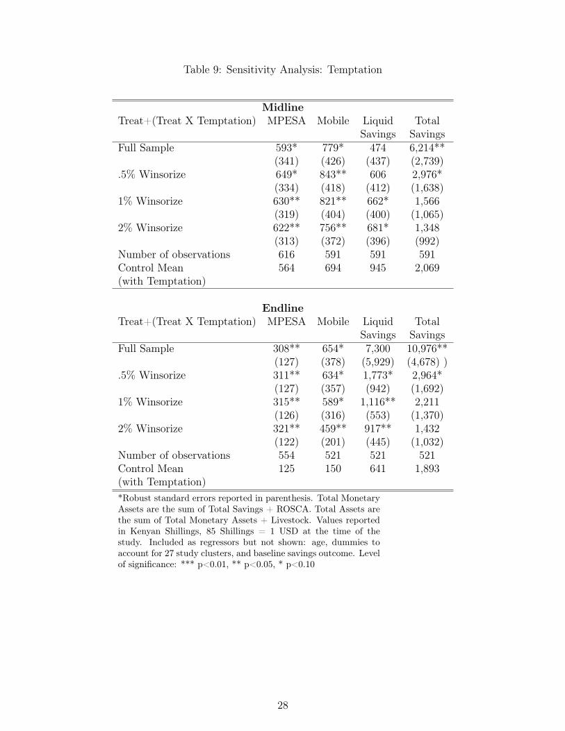
Table 9: Sensitivity Analysis: Temptation

MidlineTreat+(Treat X Temptation) MPESA Mobile Liquid Total

Savings SavingsFull Sample 593* 779* 474 6,214**

(341) (426) (437) (2,739).5% Winsorize 649* 843** 606 2,976*

(334) (418) (412) (1,638)1% Winsorize 630** 821** 662* 1,566

(319) (404) (400) (1,065)2% Winsorize 622** 756** 681* 1,348

(313) (372) (396) (992)Number of observations 616 591 591 591Control Mean 564 694 945 2,069(with Temptation)

EndlineTreat+(Treat X Temptation) MPESA Mobile Liquid Total

Savings SavingsFull Sample 308** 654* 7,300 10,976**

(127) (378) (5,929) (4,678) ).5% Winsorize 311** 634* 1,773* 2,964*

(127) (357) (942) (1,692)1% Winsorize 315** 589* 1,116** 2,211

(126) (316) (553) (1,370)2% Winsorize 321** 459** 917** 1,432

(122) (201) (445) (1,032)Number of observations 554 521 521 521Control Mean 125 150 641 1,893(with Temptation)*Robust standard errors reported in parenthesis. Total MonetaryAssets are the sum of Total Savings + ROSCA. Total Assets arethe sum of Total Monetary Assets + Livestock. Values reportedin Kenyan Shillings, 85 Shillings = 1 USD at the time of thestudy. Included as regressors but not shown: age, dummies toaccount for 27 study clusters, and baseline savings outcome. Levelof significance: *** p<0.01, ** p<0.05, * p<0.10

28

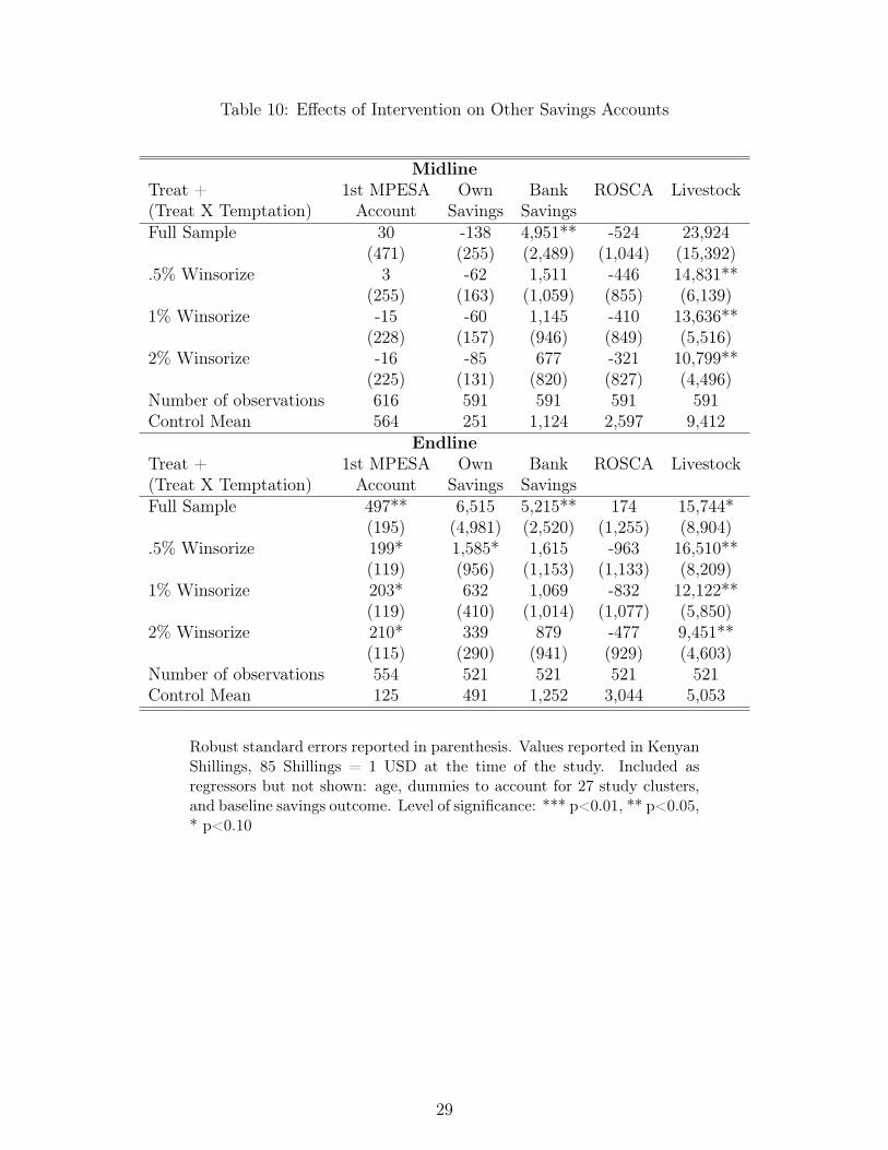
Table 10: Effects of Intervention on Other Savings Accounts

MidlineTreat + 1st MPESA Own Bank ROSCA Livestock(Treat X Temptation) Account Savings SavingsFull Sample 30 -138 4,951** -524 23,924

(471) (255) (2,489) (1,044) (15,392).5% Winsorize 3 -62 1,511 -446 14,831**

(255) (163) (1,059) (855) (6,139)1% Winsorize -15 -60 1,145 -410 13,636**

(228) (157) (946) (849) (5,516)2% Winsorize -16 -85 677 -321 10,799**

(225) (131) (820) (827) (4,496)Number of observations 616 591 591 591 591Control Mean 564 251 1,124 2,597 9,412

EndlineTreat + 1st MPESA Own Bank ROSCA Livestock(Treat X Temptation) Account Savings SavingsFull Sample 497** 6,515 5,215** 174 15,744*

(195) (4,981) (2,520) (1,255) (8,904).5% Winsorize 199* 1,585* 1,615 -963 16,510**

(119) (956) (1,153) (1,133) (8,209)1% Winsorize 203* 632 1,069 -832 12,122**

(119) (410) (1,014) (1,077) (5,850)2% Winsorize 210* 339 879 -477 9,451**

(115) (290) (941) (929) (4,603)Number of observations 554 521 521 521 521Control Mean 125 491 1,252 3,044 5,053

Robust standard errors reported in parenthesis. Values reported in KenyanShillings, 85 Shillings = 1 USD at the time of the study. Included asregressors but not shown: age, dummies to account for 27 study clusters,and baseline savings outcome. Level of significance: *** p<0.01, ** p<0.05,* p<0.10

29

Table 11: Midline Temptation Expenses

Temptation Share of Food ExpSpending on Temptation Goods

Treat -215* -250** -0.02* -0.02*(128) (124) (0.01) (0.01)

Control: Baseline Temptation Spending Yes Yes Yes YesControl: Baseline Total Savings No Yes No YesNumber of observations 111 111 111 111Control Mean 461 0.03

Robust standard errors reported in parenthesis. Temptation Spending ag-gregates all spending on hairdressing and cosmetics from 12 weekly surveysconducted between baseline and midline. Share of Food Exp on TemptationGoods takes Temptation Spending and divides this by all food expendituresfrom the 12 weekly surveys. Baseline temptation spending is included asa control in all specifications. Values reported in Kenyan Shillings, 85Shillings = 1 USD at the time of the study. Included as regressors but notshown: age, dummies to account for 27 study clusters, and baseline savingsoutcome. Level of significance: *** p<0.01, ** p<0.05, * p<0.10

30

Table 12: SMS Reminders

MPESA Mobile Liquid Total SavingsSMS Reminders 147 175 2,157 -156

(134) (155) (1,841) (1,319).5% Winsorize 149 147 373 -85

(132) (147) (280) (692)1% Winsorize 137 140 237 508

(127) (143) (224) (549)2% Winsorize 126 112 194 629

(123) (134) (205) (516)Number of observations 267 250 250 250Control Mean 712 891 1,565 2,887

31

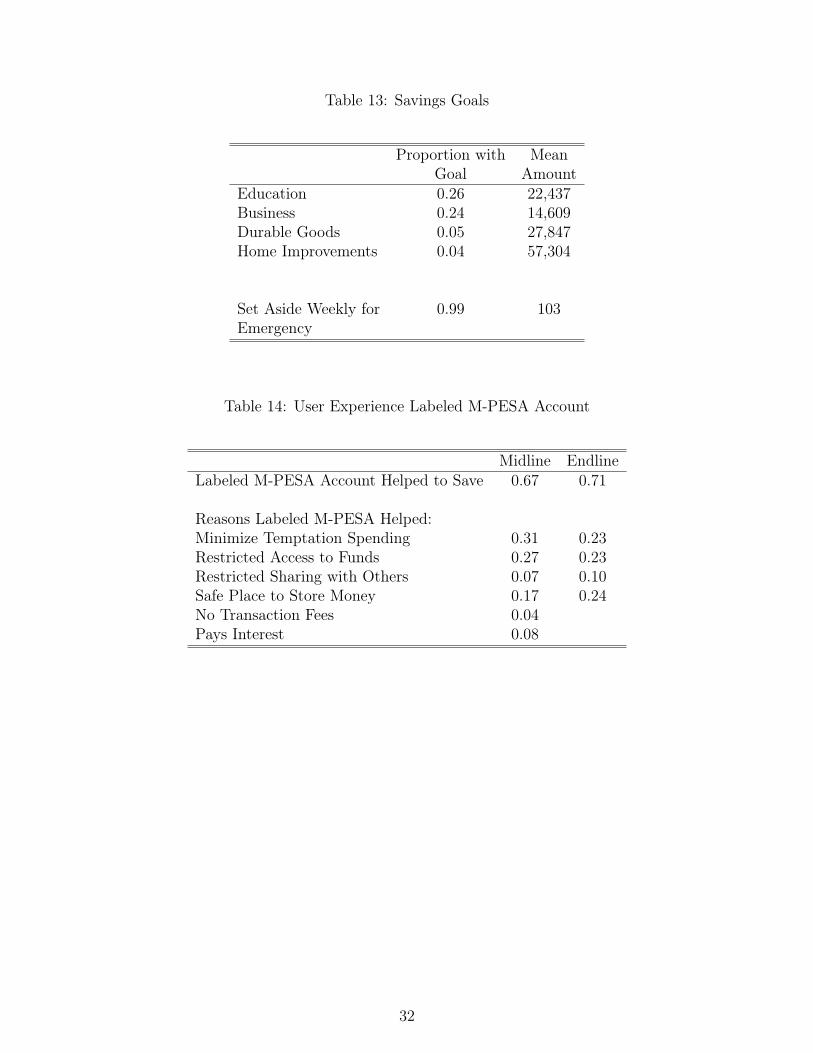
Table 13: Savings Goals

Proportion with MeanGoal Amount

Education 0.26 22,437Business 0.24 14,609Durable Goods 0.05 27,847Home Improvements 0.04 57,304

Set Aside Weekly for 0.99 103Emergency

Table 14: User Experience Labeled M-PESA Account

Midline EndlineLabeled M-PESA Account Helped to Save 0.67 0.71

Reasons Labeled M-PESA Helped:Minimize Temptation Spending 0.31 0.23Restricted Access to Funds 0.27 0.23Restricted Sharing with Others 0.07 0.10Safe Place to Store Money 0.17 0.24No Transaction Fees 0.04Pays Interest 0.08

32

A Appendix

Table A.1: Sensitivity Analysis: Winsorized Sample

MidlineTreat MPESA Mobile Liquid Total SavingsFull Sample 404 290 317 1,884**

(295) (316) (370) (929).5% Winsorize 126 -8 25 851

(205) (230) (274) (624)1% Winsorize 144 11 27 114

(160) (189) (224) (481)2% Winsorize 156 -12 -21 29

(145) (163) (197) (426)Number of observations 616 591 591 591Control Mean 1,185 1,429 1,775 2,903hline

EndlineTreat MPESA Mobile Liquid Total SavingsFull Sample 26 8 1,374 3,615**

(141) (187) (1,620) (1,835).5% Winsorize 40 12 -47 264

(136) (181) (297) (554)1% Winsorize 80 20 -111 68

(126) (170) (217) (513)2% Winsorize 148 94 -69 -67

(100) (127) (187) (405)Number of observations 554 521 521 521Control Mean 712 891 1,565 2,887

Robust standard errors reported in parenthesis. Values reported in KenyanShillings, 85 Shillings = 1 USD at the time of the study. Included asregressors but not shown: age, dummies to account for 27 study clusters,and baseline savings outcome. Level of significance: *** p<0.01, ** p<0.05,* p<0.10

33

Table A.2: Sensitivity Analysis: Treatment Effects on Social Appropriation Sample

MidlineMidine

Linear combination MPESA Mobile Liquid Total SavingsTreat+(Treat X Social Approp.)Full Sample 905** 677 425 -3,132

(391) (477) (570) (2,373).5% Winsorize 849** 707* 519 -1,446

(362) (424) (496) (1,367)1% Winsorize 732** 599* 492 -698

(314) (353) (422) (1,071)2% Winsorize 709** 581* 485 -494

(308) (334) (403) (981)Number of observations 616 591 591 591Control Mean 238 295 665 1,942

EndlineLinear combination MPESA Mobile Liquid Total SavingsTreat+(Treat X Social Approp.)Full Sample 331* 403* 170 -3,826

(192) (224) (596) (3,100).5% Winsorize 325* 403* 153 -86

(191) (224) (518) (1,241)1% Winsorize 306 392* 153 79

(186) (221) (483) (1,271)2% Winsorize 293* 379* 160 121

(175) (209) (476) (1,205)Number of observations 554 521 521 521Control Mean 181 174 1,145 1,991

Robust standard errors reported in parenthesis. Values reported in KenyanShillings, 85 Shillings = 1 USD at the time of the study. Included asregressors but not shown: age, dummies to account for 27 study clusters,and baseline savings outcome. Level of significance: *** p<0.01, ** p<0.05,* p<0.10

34