Chapter 1

Mendel

In the middle of the nineteenth century, an Austrian monk, Gregor Mendel,toiled for almost 10 years systematically breeding pea plants and recording hisresults. Like many of his contemporaries, Mendel was intrigued with heredityand wanted to uncover the laws behind it. In 1864, just five years after thepublication of Charles Darwin’s Origin of Species, Mendel presented his resultsto the local natural history society in Brünn1 which published his paper in theirproceedings one year later (Mendel, 1865).

Figure 1.0.1: Gregor Mendel at age c.40.

Image from http://en.wikipedia.org/wiki/Gregor_Mendel

To be honest, many historians sur-mise that Mendel’s presentation andhis paper were quite boring. Theywere crammed with numbers and per-centages about green versus yellowpeas, round versus wrinkled peas, ax-ial versus terminal infloresences, yel-low versus green pods, red-brown ver-sus white seed coats, etc. To makematters worse, many of these traitswere cross-tabulated. Hence, his au-dience had to listen to numbers aboutround and yellow versus wrinkled and yellow versus round and green versuswrinkled and green pea plants.

Perhaps as a consequence of this, no one paid attention to Mendel, and thebasic principles of genetics that he elucidated in his presentation and subsequentpaper went unrecognized until shortly after the turn of the 20th century. Today,a Mendelian trait is a trait due to a single gene that follows classic Mendeliantransmission. Likewise, a Mendelian disorder is one influenced by a single locus.In this chapter, we examine what Mendel accomplished and the terminology thathas evolved to relate a single gene to an observed trait.

1During Mendel’s time, Brünn was the capital of Moravia in the Austro-Hungarian empire.Today, it is called Brno and is in the Czech Republic. Mendel’s monastery and pea gardenare popular tourist destinations.

1

1.1. THE LAW OF DOMINANCE CHAPTER 1. MENDEL

Table 1.1: Mendel’s three laws.

Law ExplanationDominance When two different hereditary factors are present, one

will be dominant and the other will be recessive.

Segregation Hereditary factors are discrete. Each organism has twodiscrete hereditary factors and passes one of these, atrandom, to an offspring.

IndependentAssortment

The discrete hereditary factors for one trait (e.g., color ofpea) are transmitted independently of the hereditaryfactors for another trait (e.g., shape of pea).

Mendel postulated three laws: (1) dominance, (2) segregation, and (3) inde-pendent assortment. Table 1.1 presents these laws and their definitions. Firstnote the phrase “hereditary factor” in the table. This is the term that Mendelused in his original paper. The term gene was coined in 1909 by the Danishbotanist Wilhelm Johannsen.

In the following sections, we will examine some of Mendel’s actual data andtry to deduce how Mendel may have arrived at them.

1.1 The law of dominance

Figure 1.1.1: Mendel’s cross for roundand wrinkled peas.

Figure 1.1.1 presents the results ofone of Mendel’s breeding experi-ments. Mendel began with two linesof yellow peas that always bred true.One line consistently gave round peaswhile the second always gave wrinkledpeas. In a classic Mendelian cross,this is called the parental generationand two strains are abbreviated as P1and P2.

Mendel cross bred these twostrains by fertilizing the round strainwith pollen from the wrinkled strainand fertilizing the wrinkled strainwith pollen from the round plants.Tis generates what is called the firstfilial generation or F1. The seedsfrom the next generation were allround. At this point, Mendel prob-

ably asked himself, “Whatever happened to the hereditary information aboutmaking a wrinkled pea?”Mendel did not stop at this point. He cross-fertilized

2

CHAPTER 1. MENDEL 1.2. THE LAW OF SEGREGATION

all the pea plants in this generation with pollen from other plants in the samegeneration. When their progeny matured, he noticed a very curious phe-nomenon—wrinkled peas reappeared! How could this happen when all theparents of these plants had round seeds? Obviously, the middle generationin Figure 1.1.1, despite being all round, still possessed some hereditary informa-tion for making a wrinkled pea. But somehow that information was not beingexpressed. Hence, Mendel surmised, some hereditary factors are dominant toother hereditary factors. In this case, a round shape is dominant to a wrinkledshape.

1.2 The law of segregation

Figure 1.1.1 gives the number and percentage of round and wrinkled peas in thethird generation, technically called the second filial generation and abbreviatedas F2. There were just about three round seeds for every wrinkled seed. Thisratio of 3 plants with the dominant hereditary factor to every one plant withthe recessive factor kept coming up time and time again in Mendel’s breedingprogram. There were 3.01 yellow seeds for every green seed; 3.15 colored flowersto every white flower; 2.95 inflated pods to every constricted pod. Mendel musthave spent considerable time cogitating over a sound, logical reason why this3:1 ratio should always appear.

To answer this question, let us return to Figure 1.1.1 and consider the mid-dle generation in light of the law of dominance. Obviously, because they arethemselves round, these plants must have the hereditary information to make around pea. They must also have the hereditary information to make a wrinkledpea because one quarter of their progeny are wrinkled. Hence, these peas havetwo pieces of hereditary information. Mendel’s stroke of genius lay in apply-ing elementary probability theory to this generation—what would one expect ifthese two types of hereditary information were discrete and combined at randomin the next generation?

The situation for this is depicted in Table 9.2 where R denotes the hereditaryinformation for making a round pea and W, the information for a wrinkledpea. The probability that a plant in the middle generation transmits the Rinformation is simply the probability of a heads on the flip of a coin or 1/2.Thus, the probability of transmitting the W information is also 1/2. Hence, theprobability that the male parent transmits the R information and the femaleparent also transmits the R information is 1/2 x 1/2 = 1/4. All of the progenythat receive two Rs will be round.

Similarly, the probability that the male transmits R while the female trans-mits W is also 1/2 x 1/2 = 1/4 as is the probability that the male transmits Wand the female, R. Thus, 1/4 + 1/4 = 1/2 of the offspring will have both the Rand the W information. They, however, will all be round because R dominatesW. At this point, Mendel’s model predicts that 3/4 of all the offspring will beround.

The only other possibility in Table 1.2is that both the male and female

3

1.3. LAW OF INDEPENDENT ASSORTMENT CHAPTER 1. MENDEL

Table 1.2: Expectation of round and wrinkled peas in the second filial genera-tion.

Female Parent:Male Parent: Factor Prob. Factor Prob.

Factor Prob. R 1/2 W 1/2R 1/2 RR 1/4 RW 1/4W 1/2 WR 1/4 WW 1/4

plant will transmit W. The probability of this is also 1/2 x 1/2 = 1/4. So theremaining 1/4 of the progeny will receive only the hereditary information onmaking a wrinkled pea and consequently will be wrinkled themselves. “Voila!”Mendel must have thought, “The hereditary factors are discrete. Every planthas two hereditary factors and passes only one, at random, to an offspring.” Insuch a breeding design, the “grandpeas” will always have a 3:1 ratio of dominanttrait to recessive trait.

1.3 Law of independent assortment

A scientist who achieves success using one particular technique always uses thattechnique in the initial phase of solving the next problem. Mendel was probablyno exception. His success in using the mathematics of probability to developthe law of segregation undoubtedly influenced his approach to his next problem,that of dealing with two different traits at once.

Figure 1.3.1: Mendel’s dihybrid cross:Pea shape (round v. wrinkled) and peacolor (yellow v. green).

Figure 1.3.1 gives the results ofhis breeding round, yellow plants withwrinkled green plants and keepingtrack of both color and shape in thesubsequent generations. The middlegeneration is all yellow and round.Hence, yellow is the dominant heredi-tary factor for color; and round, as wehave seen, is the dominant for shape.The next generation is both confirma-tory and troubling. First, there are atotal of 423 round and 133 wrinkledpeas, giving a ratio of 3.18 to 1, veryclose to the 3:1 ratio expected fromthe laws of dominance and segrega-tion. Also confirming these predic-tions is the 2.97 to 1 ratio of yellowto green peas.

This generation, however, hascombinations of traits not seen in either of the previous generations—wrinkled,

4

CHAPTER 1. MENDEL 1.3. LAW OF INDEPENDENT ASSORTMENT

Table 1.3: Gametes and their probabilities from an F1 plant in a dihybrid crossof pea shape (R = round, W = wrinkled) and pea color (Y = yellow, G =green).

Color:Shape: Factor Prob. Factor Prob.

Factor Prob. Y 1/2 G 1/2R 1/2 RY 1/4 RG 1/4W 1/2 WY 1/4 WG 1/4

yellow peas and round, green peas. What can explain this? Once again, themathematics of probability gave a solution. Mendel’s hypothesis was that thehereditary factors for pea color are independent of the hereditary factors forpea shape. The mathematical calculations for deriving the expected numberof plants of each type in the third generation are more complicated than thosefor deriving the law of segregation, but they follow the same basic principles ofprobability theory.

Each plant in the F1 generation will have four discrete hereditary factors,the R and W factors that we have already discussed and the Y (for yellow)and G (for green) factors that determine color. The first step is to calculate theexpected gametes from an F1 plant under Mendel’s hypothesis of independentassortment. We have already seen that the probability that an F1 plant trans-mits, say, a round (R) hereditary factor is 1/2. By similar logic, the probabilitythat a F1 plant transmits a yellow (Y ) hereditary factor for color is also 1/2. Ifthe hereditary factors for the two traits–shape and color–are independent, thenthe probability of transmitting a gamete with a round (R) and a yellow (Y )factor equals the product of these two probabilities or 1/2 ⇥ 1/2 = 1/4. Table1.3 enumerates all possible gametes, along with their probabilities, from an F1plant in this dihybrid cross. The four possible gametes are RY, WY, RG, andWG and the probability of each one equals 1/4.

The next step is to tabulate the probable outcomes in the F2. These can becomputed by enumerating all possible gametes from the female as a function ofall possible gametes from the male plant. With four possible gametes from thefemale and four from the male, there will be 16 different possible outcomes inthe F2. The probability of each is 1/4 ⇥ 1/4 = 1/16. Figure 1.3.2 shows theseoutcomes by genotype and, graphically, the observed traits. To construct theobserved traits, recall that round (R) is dominant to wrinkled (W ) and yellow(Y ) is dominant to green (G).

We can see now why there are combinations of observed traits in the F2 thatwere not present in either of the original parental plants. Consider the secondrow and second column of the probable offspring in Figure 1.3.2. These offspringare yellow and wrinkled, a combination not seen in the original parents (see thetwo parental strains in Figure 1.3.1). These plants came about because boththe male and female in the F1 generation transmitted the W hereditary factorthey received from their green, wrinkled parent but the Y color factor that they

5

1.4. MENDEL’S LAWS: EXCEPTIONS CHAPTER 1. MENDEL

Figure 1.3.2: Enumeration of outcomes in the F2 from a dihybrid cross of peashape (R = round, W = wrinkled) and pea color (Y = yellow, G = green).

received from their other parent–the yellow, round one.The predicted outcomes in Figure 1.3.2 also closely agree with the observed

outcomes from Figure 1.3.1 Nine-sixteenths of the offspring are expected tobe round and yellow, three-sixteenths will be round and green, another three-sixteenths will be wrinkled and yellow, and the remaining one-sixteenths shouldbe wrinkled and green. Indeed, this expected 9:3:3:1 ratio is very close thatobserved by Mendel. Were this to happen today, Mendel would have high-fived all the monklettes who helped him to plant and to count the peas (andprobably to harvest and dine on them as well) and dashed off a paper to Scienceor Nature.2 Instead, he patiently tabulated his results and embarked on thejourney to Brünn.

1.4 Mendel’s laws: Exceptions

The majority of seminal scientific discoveries never get things completely right.Instead, they turn science in a different direction and make us think aboutproblems in a different way. It often takes years of effort to fill in the fine pointsand find the exceptions to the rule. Mendel’s laws follow this pattern. None ofthe three laws is completely correct. We know now that some hereditary factorsare codominant, not completely dominant, to others–one can cross red withwhite petunias and get pink offspring, not the red or white ones that Mendelwould have predicted.

We also know that the law of segregation is not always true in its literalsense. In humans, the X and the Y chromosome are indeed discrete, but theynot passed along entirely at random from a father—slightly more boys than girlsare conceived.

2Science and Nature are the two most prestigious science journals in the world today.

6

CHAPTER 1. MENDEL 1.5. TERMINOLOGY

Finally, we also know that not all hereditary factors assort independently.Those that are located close together on the same chromosome tend to be in-herited as a unit, not as independent entities.

These exceptions, however, are individual trees within the forest. Mendel’sgreat accomplishment was to orient science toward the correct forest. Hereditaryfactors do not “blend” as Darwin and others of his time thought; they are discreteand particulate, as Mendel postulated. As Mendel conjectured, we have twohereditary factors, one of which we received from our father and the other fromour mother. We do not have 23 hereditary factors, one on each chromosome,as the early cell biologist Weissman theorized. And two different hereditaryfactors, provided that they are far enough away on the same chromosome orlocated on entirely different chromosomes, are transmitted independently ofeach other. Mendel’s basic concepts provided a paradigm shift and sparked thenascent science of genetics at the turn of the century, an achievement that thehumble monk was never recognized for during his life.

1.5 Terminology

Before we continue, some terminology is in order. In molecular biology, whatMendel called an “hereditary factor” is now known as a gene. The molecularbiology definition of a gene is a section of DNA that contains the blueprint fora polypeptide chain. The term locus (plural = loci) is a synonym for a gene.

A gene may be either monomorphic or polymorphic. To grasp the meaningsof these two terms, imagine that we obtained the nucleotide sequence of a geneon all of humanity. A monomorphic gene is one in which the sequence of As,Cs, Gs, and Ts is the same for all strands of DNA. A polymorphic gene is one inwhich there are several common “spelling variations” of the gene. Arbitrarily,“common” is defined as a nucleotide sequence with a prevalence of 1% of higher.

The spelling variations at a gene are called alleles. Unfortunately, manygeneticists also use the term gene to refer to an allele, sowing untold confusionamong beginning genetics’ students, so let us examine a specific case to explainthe technical difference between a gene and an allele.

The ABO gene (or ABO locus) is a stretch of DNA close to the bottomof human chromosome 9 that contains the blueprint for an protein that sitswithin the plasma membrane of red blood cells. Not all of us, however, havethe identical sequence of the A, T, C and G nucleotides along this DNA sequence.There are spelling variations or alleles that exist in the human gene pool at theABO locus. The three most common alleles are the A allele, the B allele, andthe O allele.

Because we all inherit two number nine chromosomes—one from mom andthe other from dad—we all have two copies of the ABO locus. By chance,the spelling variation at the ABO stretch of DNA on dad’s chromosome maybe the same as the spelling variation at this region on mom’s chromosome.An organism like this is called a homozygote (homo for "same" and zygote for"fertilized egg"). The strict definition of a homozygote is an organism that

7

1.5. TERMINOLOGY CHAPTER 1. MENDEL

has the same two alleles at a gene. For the ABO locus, those who inherittwo A alleles are homozygotes as are those who inherit two B alleles or twoO alleles. A heterozygote is an organism with different alleles at a locus. Forexample, someone who inherits an A allele from mom but a B allele from dadis a heterozygote.

Wilhelm Johanssen (1909), the person who coined the term gene, also pro-posed an important distinction between the genotype and the phenotype. Thegenotype is defined as the two alleles that a person (or group of people) hasat a locus. At the ABO locus, the genotypes are AA, AB, AO, BB, BO, andOO. (There is a tacit understanding that the heterozygotes AO and OA are thesame genotype.) The word “genotype” may also be used as a vague designationof genetic predisposition without identifying either the genes or the alleles. Asexample is the statement “he has the genotype for obesity.”

A phenotype is defined as the observed characteristic or trait. Height, weight,extraversion, intelligence, interest in blood sports, memory, and shoe size areall phenotypes.

There is not always a simple, one-to-one correspondence between a genotypeand a phenotype. For example, there are four phenotypes at the ABO bloodgroup—A, B, AB, and O. These phenotypes come about when a drop of blood isexposed to a chemical that reacts to the molecule produced from the A enzymeand then to another chemical that reacts specifically to the enzyme producedfrom a B allele. (The O allele produces no viable enzyme, so there is no reaction).

If someone takes a drop of your blood, adds the A chemical to it, and observesa reaction, then it is clear that you must have at least one A allele—although,of course, you may actually have two A alleles. If the person takes another dropof your blood, adds the B chemical, and observes a reaction, and then you musthave phenotype AB. In this case, your genotype must also be AB. If a reactionoccurs to the A chemical but not to the B chemical, then you have phenotypeA but could be genotype AA or genotype AO—the test cannot distinguish oneof these genotypes from the other. Similarly, if your blood fails to react to theA chemical but reacts to the B chemical, then you are phenotype B, although itis uncertain whether your genotype is BB or BO. When there is no reaction toeither the A or the B chemical, and then the phenotype is O and the genotypeis OO.

Finally, there are several terms used to describe allele action in terms ofthe phenotype that is observed in a heterozygote. When the phenotype of aheterozygote is the same as the phenotype of one of the two homozygotes, thenthe allele in the homozygote is said to be dominant and the allele that is "notobserved" is termed recessive. Because the heterozygote with the genotype AOhas the same phenotype as the homozygote AA, then allele A is dominant andO is recessive. Similarly, allele B is dominant to O, or in different words, alleleO is recessive to B.

When the phenotype of the heterozygote takes on a value somewhere be-tween the two homozygotes, then allele action is said to be partially dominant,incompletely dominant, additive, or codominant. Because the genotype AB givesa different phenotype from both genotypes AA and BB, one would say that al-

8

CHAPTER 1. MENDEL1.6. APPLICATION OF MENDEL’S LAWS: THE PUNNETT

RECTANGLE

leles A and B are codominant with respect to each other. (The term additivewould equally apply, but this phrase is usually used when the phenotypes arenumbers and not qualities.) Note carefully that allele action is a relative andnot an absolute concept. For example, the allele action of A depends entirelyon the other allele—it is dominant to O but codominant to B.

1.6 Application of Mendel’s laws: The Punnett

rectangle

In high school biology, you were all exposed to a Punnett square. Indeed,the Tables1.3 and 1.2 as well as 1.3.2 are all examples of Punnett squares. Thiselementary technique was developed by Reginald Punnett who in 1905 arguablywrote the first textbook of genetics (Punnett, 1905).

High school has also taught us that a square is a specific case of a moregeneral geometric form, the rectangle. We can now generalize and developthe concept of a Punnett rectangle to apply Mendel’s concepts of heredity tocalculating the genotypes and phenotypes of offspring from a given mating type.The advantages of of a rectangle are that it can deal with more genetic situationsthan a square and it can do so with greater efficiency. The generic steps forconstructing a Punnett rectangle are listed in Table 1.4. Let us examine thesesteps with a simple example.

1.6.1 A simple example

Consider the mating of woman who has genotype AO at the ABO blood grouplocus and a man who also has genotype AO. From Step 1 in Table 1.4, themother’s egg can contain either allele A (with a probability of 1/2) or allele O(also with a probability of 1/2). From Step 2, the father’s sperm may containeither A or O , each with a probability of 1/2. The row and column labels forthis Punnett rectangle given in Table 1.5.

Step 3 requires entry of the offspring genotypes into the cells of the rectangle.The upper left cell represents the fertilization of mother’s A egg by father’sA sperm, so the genotypic entry is AA. The upper right cell represents thefertilization of mother A egg by father’s O sperm, giving genotype AO. Followingthese rules, the genotypes for the lower left and lower right cells are, respectively,OA and OO.

We are now at Step 4 in Table 1.6–calculating the probabilities of the off-springs’ genotypes. To do this we multiply the row probability by the columnprobability. For the upper left cell, the row probability is 1/2 and the columnprobability is also 1/2, so the cell probability is 1/2 x 1/2 = 1/4. It is obviousthat each cell for this example will have a probability of 1/4. The completedPunnett rectangle is given in Table 1.6.

In Steps 5 and 6, we must complete a table of genotypes and, if needed, phe-notypes. To complete Step 5, we note that there are three unique genotypes inthe cells of the Punnett rectangle—AA, AO, and OO (remember that genotype

9

1.6. APPLICATION OF MENDEL’S LAWS: THE PUNNETTRECTANGLE CHAPTER 1. MENDEL

Table 1.4: Steps in using a Punnett rectangle to compute the distribution ofoffspring genotypes and phenotypes from a parental mating.

Step Operation

1 Write down the genotypes of the mother’s gametes along withtheir associated probabilities. These will label the rows of therectangle.

2 Write down the genotypes of the father’s gametes along withtheir associated probabilities. These will label the columns ofthe rectangle. (Naturally, it is possible to switch thesteps—mother’s gametes forming the columns and father’sgametes, the rows—without any loss of generality.)

3 The genotype for each cell within the rectangle is thegenotype of the row gamete united with the genotype of thecolumn gamete. Enter these for all cells in the rectangle.

4 The probability for each cell within the rectangle equals theprobability of the row gamete multiplied by the probability ofthe column gamete. Enter these for all cells in the rectangle.

5 Make a table of the unique genotypes of the offspring andtheir probabilities. If a genotype occurs more than oncewithin the cells of the Punnett rectangle, then add the cellprobabilities together to get the probability of that genotype.

6 If needed, make a table of the unique phenotypes and theirprobabilities from the table of genotypes. If two or moregenotypes in the genotypic table give the same phenotype,then add the probabilities of those genotypes together to getthe probability of the phenotype.

Table 1.5: Steps 1 and 2 in constructing a Punnett rectangle.

Male Gamete:Female Gamete: Allele Prob. Allele Prob.Allele Prob. A 1/2 O 1/2

A 1/2O 1/2

10

CHAPTER 1. MENDEL1.6. APPLICATION OF MENDEL’S LAWS: THE PUNNETT

RECTANGLE

Table 1.6: Results of a Punnett rectangle after Step 4.

Male Gamete:Female Gamete: Allele Prob. Allele Prob.Allele Prob. A 1/2 O 1/2

A 1/2 AA 1/4 AO 1/4O 1/2 OA 1/4 OO 1/4

Table 1.8: Expected genotypes and phenotypes and their frequencies from amating of an AO women and an AO man.

Genotype Frequency Phenotype Frequency

AA 1/4 A 3/4AO 1/2 O 1/4OO 1/4

OA is the same as AO). Genotypes AA and OO occur only once, so the proba-bility of each of these genotypes is 1/4. Genotype AO, on the other hand, occurstwice, once in the upper right cell and again in the lower left. Consequently, theprobability of the heterozygote AO is the sum of these two cell probabilities or1/4 + 1/4 = 1/2. Table 1.7 gives the genotypes and their frequencies for theoffspring of this mating.

Table 1.7: Expected offspring genotypesand their frequencies.

Genotype Frequency

AA 1/4AO 1/2OO 1/4

Step 6 requires calculation of thephenotypes from the genotypes. Be-cause allele A is dominant in theABO blood system, both genotypesAA and AO will have phenotype A.The probability of phenotype A willbe the sum of the probabilities forthese two genotypes or 1/4 + 1/2 =3/4. Genotype OO will have pheno-type O. Because genotype OO occursonly once, the probability of pheno-type O is simply 1/4. The complete table of genotypic and phenotypic frequen-cies is given in Table 1.8.

1.6.2 A two-locus example

The logic of the Punnett rectangle may be applied to genotypes at more thanone locus. The only requirement is that all the loci are unlinked, i.e., no two lociare located close together on the same chromosome. (Later on, we deal withthe case of Punnett rectangles with linked loci.)

The Punnett rectangle for two loci will be illustrated by calculating tradi-

11

1.6. APPLICATION OF MENDEL’S LAWS: THE PUNNETTRECTANGLE CHAPTER 1. MENDEL

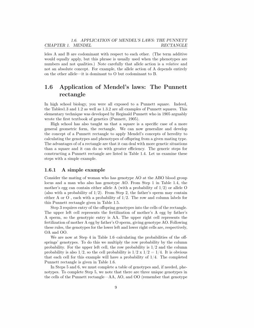
Table 1.9: Mothers’s gametes and probabilities.

Rhesus Locus:ABO Locus: Allele Prob. Allele Prob.

Allele Prob. + 1/2 - 1/2O 1.0 O+ 1/2 O- 1/2

tional blood types. Traditional blood-typing for transfusions uses phenotypes attwo genetic loci. The first is the ABO locus and the second is the Rhesus locus.Although the genetics of the Rhesus locus are actually quite complicated, wewill assume that there are only two alleles, a “plus” or + allele and a “minus”or - allele . The + allele is dominant to the - allele, so the two Rhesus pheno-types are + and -. The blood types used for transfusions and blood donationsconcatenate the ABO phenotype with the Rhesus phenotype, giving phenotypessuch as A+, B-, AB+, etc. Our problem? What are the expected frequencies forthe offspring of a father with genotype AO/+- (read “genotype AO at the ABOlocus and genotype +- at the Rhesus locus”) and a mother who is genotypeOO/+-?

The trick to the problem of two unlinked loci is to go through the Punnettrectangle steps three times. In the first pass, the Punnett rectangle is used toobtain the genotypes for the maternal gametes. The second pass calculates thepaternal gametes, and the third and final pass uses the results from the firsttwo passes to get the offspring genotypes.

The mother in this problem has genotype OO/+-. Because the ABO andrhesus loci are unlinked, the probabilities for the ABO locus are independent ofthose for the rhesus locus. This permits us to use a Punnett rectangle to derivethe maternal gametes. The rows of the rectangle are labeled by the contributionto the maternal egg from mother’s ABO alleles and their probabilities. Here,mother can give only an O. Consequently there will be only one row to therectangle, and it will be labeled O and have a probability of 1.0. The columnsare labeled by the contribution of mother’s rhesus alleles and their probabilities.In the present case, the columns will be labeled + and -, each with probability1/2. The completed Punnett rectangle needed to get the maternal gametes andtheir probabilities is given below in Table 1.9.

From this table, we see that there are two possible maternal gametes, eachwith a probability of 1/2. The first has one of mother’s O alleles at the ABOlocus and the + allele at the Rhesus locus, giving gamete O+. The secondgamete, O-, contains one of mothers O alleles but her - allele at Rhesus.

The second pass through the Punnett rectangle is used to calculate father’sgametes. His contribution to the gamete from his alleles at the ABO locus maybe either allele A, with probability 1/2, or O, also with probability 1/2. Thus,there will be two rows to father’s Punnett rectangle, one labeled A and the otherlabeled O, each with probability 1/2. Like mother, father is a heterozygote atRhesus. Hence the columns for his table will equal those for the maternal table.The Punnett rectangle for the paternal gametes is given below in Table 9.11.

12

CHAPTER 1. MENDEL1.6. APPLICATION OF MENDEL’S LAWS: THE PUNNETT

RECTANGLE

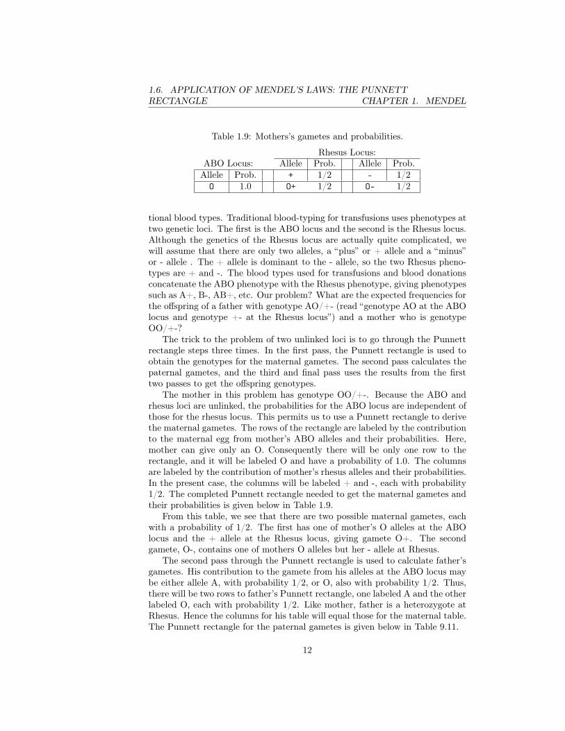
Table 1.10: Father’s gametes and probabilities.

Rhesus Locus:ABO Locus: Allele Prob. Allele Prob.

Allele Prob. + 1/2 - 1/2A 1/2 A+ 1/4 A- 1/4O 1/2 O+ 1/4 O- 1/4

Father has four different paternal gametes, each with a probability of 1/4.The first possible gamete carries father’s A allele at the ABO locus and father’s+ allele at the Rhesus locus (A+). Analogous interpretations apply to theremaining three gametes—A-, O+, and O-.

We may now construct the last Punnett rectangle to find the offspring geno-types and their frequencies. In this rectangle, the rows are labeled by thematernal gametes and their probabilities and the columns by the paternal ga-metes and their probabilities. This will give a rectangle with two rows and fourcolumns. This rectangle (with rows and columns switched for efficiency) is givenin Table 1.11.

Because the ordering of the alleles for a heterozygote is immaterial, genotypesAO, +- and AO, -+ in Table 1.11 are identical. So are genotypes OO, +- and OO,-+. Hence, the table of expected genotypes can be written as the one in Table1.12. The table also gives the phenotypes associated with the genotypes. Addingtogether those rows with identical phenotypes gives the following phenotypicfrequencies: 3/8 or 37.5% of the offspring are expected to have blood type A+;1/8 or 12.5% will have blood type A-; 3/8 or 37.5% will have blood type O+;and 1/8 or 12.5% will have blood type O-.

1.6.3 X-linked loci

In mammals, genetic females have two X chromosomes while genetic males haveone X chromosome and one Y chromosome. The Y chromosome is much smallerthan the X chromosome and contains many fewer loci than the X. Thus, manygenes on the X chromosome—in fact, the overwhelming number of genes—do

Table 1.11: Expected offspring genotypes and their frequencies from an OO, +-woman and an AO, +- man.

Mother:Father: Gamete Prob Gamete Prob

Gamete Prob O+ 1/8 O- 1/4A+ 1/4 AO, ++ 1/8 AO, +- 1/8A- 1/4 AO, -+ 1/8 AO, -- 1/8O+ 1/4 OO, ++ 1/8 OO, +- 1/8O- 1/4 OO, -+ 1/8 OO, -- 1/8

13

1.7. CONCLUSIONS CHAPTER 1. MENDEL

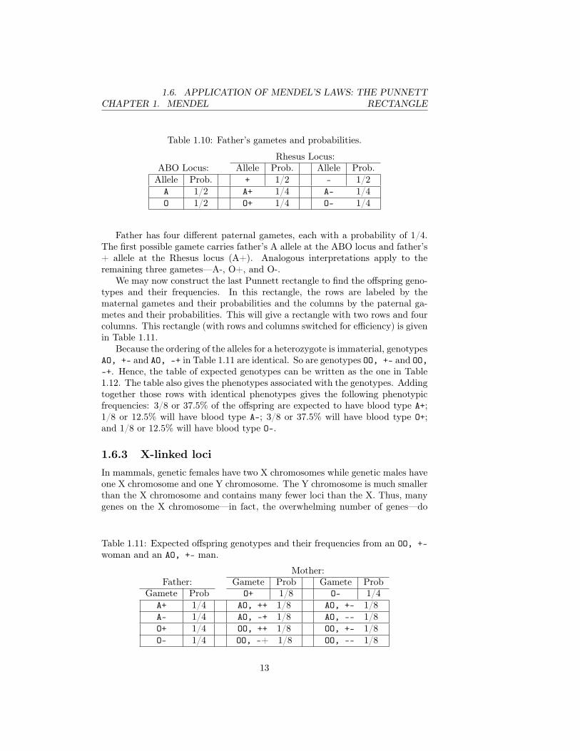
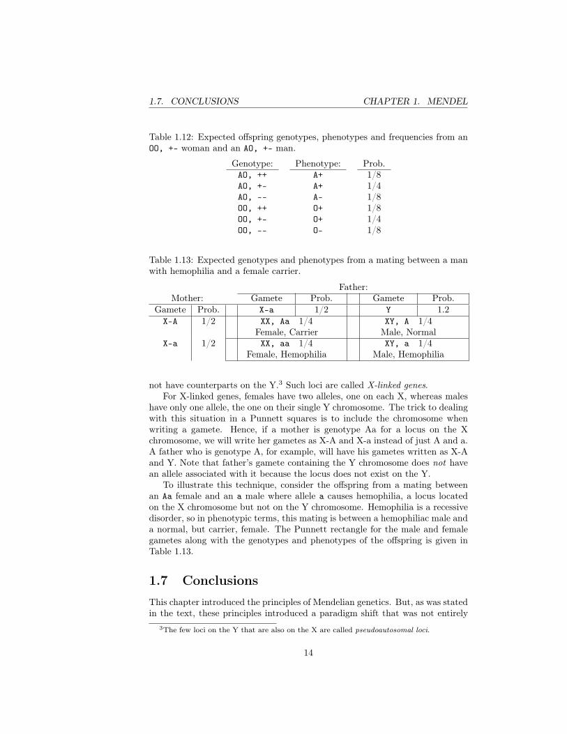
Table 1.12: Expected offspring genotypes, phenotypes and frequencies from anOO, +- woman and an AO, +- man.

Genotype: Phenotype: Prob.AO, ++ A+ 1/8AO, +- A+ 1/4AO, -- A- 1/8OO, ++ O+ 1/8OO, +- O+ 1/4OO, -- O- 1/8

Table 1.13: Expected genotypes and phenotypes from a mating between a manwith hemophilia and a female carrier.

Father:Mother: Gamete Prob. Gamete Prob.

Gamete Prob. X-a 1/2 Y 1.2X-A 1/2 XX, Aa 1/4

Female, CarrierXY, A 1/4

Male, NormalX-a 1/2 XX, aa 1/4

Female, HemophiliaXY, a 1/4

Male, Hemophilia

not have counterparts on the Y.3 Such loci are called X-linked genes.For X-linked genes, females have two alleles, one on each X, whereas males

have only one allele, the one on their single Y chromosome. The trick to dealingwith this situation in a Punnett squares is to include the chromosome whenwriting a gamete. Hence, if a mother is genotype Aa for a locus on the Xchromosome, we will write her gametes as X-A and X-a instead of just A and a.A father who is genotype A, for example, will have his gametes written as X-Aand Y. Note that father’s gamete containing the Y chromosome does not havean allele associated with it because the locus does not exist on the Y.

To illustrate this technique, consider the offspring from a mating betweenan Aa female and an a male where allele a causes hemophilia, a locus locatedon the X chromosome but not on the Y chromosome. Hemophilia is a recessivedisorder, so in phenotypic terms, this mating is between a hemophiliac male anda normal, but carrier, female. The Punnett rectangle for the male and femalegametes along with the genotypes and phenotypes of the offspring is given inTable 1.13.

1.7 Conclusions

This chapter introduced the principles of Mendelian genetics. But, as was statedin the text, these principles introduced a paradigm shift that was not entirely

3The few loci on the Y that are also on the X are called pseudoautosomal loci.

14

CHAPTER 1. MENDEL 1.8. REFERENCES

correct. Mendel’s law of dominance did not apply universally to all hereditaryfactors. This is not a major problem because we can always amend his laws toallow for “partial dominance” or “codominance.”

On the other hand, Mendel’s law of independent assortment has been demon-strated to be incorrect in a significant number of cases. A major reason is that“hereditary factors,” as Mendel called them, are not an enormous number ofindividual discrete particles within a cell. Instead, many of them appear to belinearly arranged on the physical molecules of inheritance, the chromosomes.The concept of the linear arrangement of hereditary factors is the topic of thenext exposition of quantitative genetics—linkage.

1.8 References

Johannsen, W. (1909). Elemente der exakten Erblichkeitslehre. Gustav Fisher,Jena.

Mendel, G. (1865). Versuche über pflanzen-hybriden. Verhandlungen des natur-forschenden Vereines in Brünn, Abhandlungen, 4:1–47.

Punnett, R. C. (1905). Mendelism. Bowes and Bowes, Cambridge.

15