Melissa Soenke March 11, 2014 - University of Arizona

Melissa SoenkeMarch 11, 2014

EEG data from one time point can be conceptualized as a line traveling through high dimensional space

Revisiting Chapter 10 and the Dot Product “A vector with two elements can be conceptualized as

a point in 2-D space. A vector with three elements can therefore be conceptualized as a point in a 3-D space (a cube), and so on for as many dimensions as there are elements in the vector.”

In PCA each dimension corresponds to each electrode

“The goal of PCA is to construct sets of weights (called principal components) based on the covariance of a set of correlated variables (electrodes) so that components explain all the variance of the data.”

Uncorrelated with each other

Created so the first component explains as much variance as possible for one electrode, the second as much of the residual variance as possible for one electrode while still being orthogonal to the first, and so on for as many components as there are electrodes

Geometric – each component is a vector in a space characterized by as many dimensions as there are electrodes that characterizes the direction of the data distribution

As a set of spatial filters Weights for each electrode are defined by patterns of

interelectrode temporal covariance

SURFACE LAPLACIAN PCA

Weights are defined only by statistical properties, not physical location on the scalp

Identifies large-scale covariance and highlights global spatial features of the data

Weights are defined by interelectrode distance

Attenuates low-spatial frequency activity and highlights local features of the data

As a data reduction technique High dimensional data (like our 64 electrode data)

can be reduced to a smaller number of dimensions Components that account for a large amount of

variance reflect true signal Components that account for less variance reflect

noise

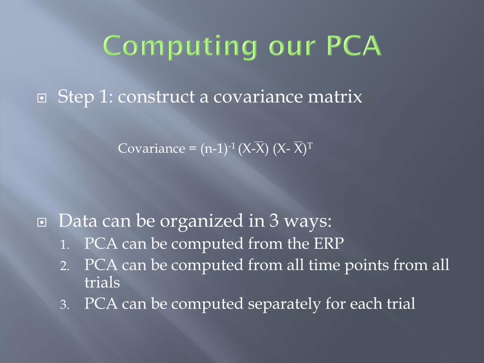
Step 1: construct a covariance matrix

Data can be organized in 3 ways:1. PCA can be computed from the ERP2. PCA can be computed from all time points from all

trials3. PCA can be computed separately for each trial

Covariance = (n-1)-1 (X-X) (X- X)T

Covariance of ERP

P1 F4 P8 P1 F4 P8

P1

F4

P8

P1

F4

P8

Average covariance of single-trial EEG

P1 F4 P8 P1 F4 P8

P1

F4

P8

P1

F4

P8

Covariance of single-trial EEG

P1 F4 P8 P1 F4 P8

P1

F4

P8

P1

F4

P8

Reflects phase-locked covariance

Reflects total (phase-locked & non-phase-locked) covariance

Step 2: Perform an eigendecomposition

Eigendecomposition is a matrix decomposition that returns eigenvectors and associated eigenvalues which characterize the patterns of interelectrode covariance

Eigenvectors and values exist in pairs An eigenvector is a direction An eigenvalue is a number, telling you how

much variance there is in the data in that direction

Let’s take a look at this visually using the following address:

http://georgemdallas.wordpress.com/2013/10/30/principal-component-analysis-4-dummies-eigenvectors-eigenvalues-and-dimension-reduction/

In PCA, the eigenvalues are the principal components or weights for each electrode that, applied to the electrode time series, produce the PCA time courses

Eigenvalues can be scaled to percentages of variance accounted for – divide each eigenvalue by the sum of all the eigenvaluesand multiply by 100

Results are square matrices with as many rows/columns as electrodes

Electrode weights for each component can be plotted as topographical maps and time courses of components can be obtained by multiplying weights of electrodes by electrode time-series data

FOR ERP FOR SINGLE TRIAL

PC #1, eigval=67.3325 PC #2, eigval=12.4658 PC #3, eigval=11.5038






To determine which components are significant you need to establish a percentage variance threshold. Components above this are significant.

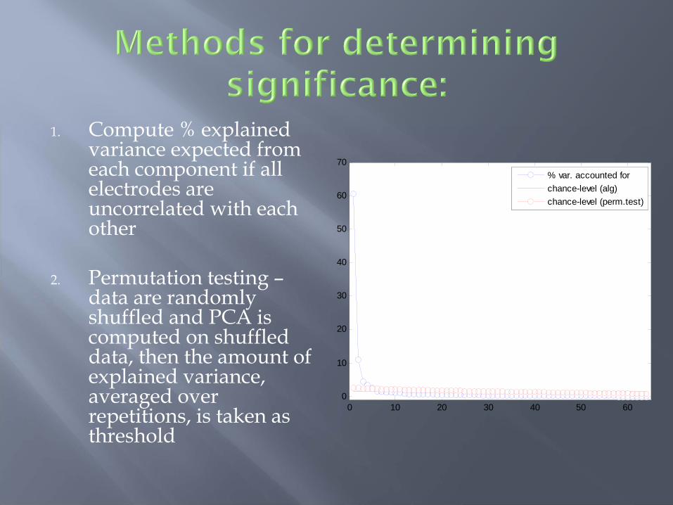
1. Compute % explained variance expected from each component if all electrodes are uncorrelated with each other

2. Permutation testing –data are randomly shuffled and PCA is computed on shuffled data, then the amount of explained variance, averaged over repetitions, is taken as threshold

0 10 20 30 40 50 600

10

20

30

40

50

60

70

% var. accounted forchance-level (alg)chance-level (perm.test)

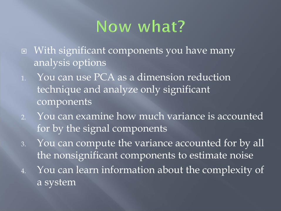
With significant components you have many analysis options

1. You can use PCA as a dimension reduction technique and analyze only significant components

2. You can examine how much variance is accounted for by the signal components

3. You can compute the variance accounted for by all the nonsignificant components to estimate noise

4. You can learn information about the complexity of a system

PCA forces components to be orthogonal

Components can be rotated to allow them to be correlated or to allow them to capture additional variance

-200 0 200 400 600 800 1000 120061.5

62

62.5

63

63.5

64

64.5

65

65.5

66

Time (ms)

% v

aria

nce

from

PC

1

PC1 from -100 ms PC1 from 200 ms PC1 from 500 ms PC1 from 1000 ms

“PCA can be combined with temporal bandpass filtering to highlight frequency-band-specific spatial features.”

First apply bandpass filter to time-domain signal, then perform PCA

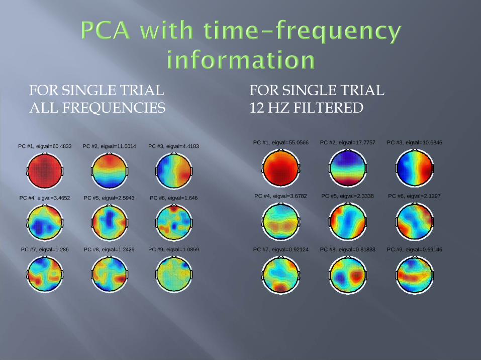
FOR SINGLE TRIALALL FREQUENCIES

FOR SINGLE TRIAL12 HZ FILTERED







PCA can be used to test condition differences PCA can be computed for all conditions

Advantage 1: signal-to-noise ratio of covariance is maximized because many trials contribute to matrix

Advantage 2: facilitates interpretation of condition differences because differences can’t be due to topographical differences in PC weights

PCA can be computed for each condition separately Advantage: increased sensitivity to identifying

condition differences because weights are tuned to each condition

State clearly the purpose of performing PCA

Clearly describe what data were used for the covariance matrices, whether filtering was applied, and what time windows were used

Melissa Soenke March 11, 2014 - University of Arizona

Documents

Transcript of Melissa Soenke March 11, 2014 - University of Arizona