Melbourne Institute Working Paper Series

Working Paper No. 1/17Estimating the Real Effects of Uncertainty Shocks at the Zero Lower Bound

Giovanni Caggiano, Efrem Castelnuovo and Giovanni Pellegrino

Estimating the Real Effects of Uncertainty Shocks at the Zero Lower Bound*

Giovanni Caggiano†, Efrem Castelnuovo‡ and Giovanni Pellegrino§

† Department of Economics, Monash University; Department of Economics and Management, University of Padova; and Bank of Finland

‡ Melbourne Institute of Applied Economic and Social Research, The University of Melbourne; Department of Economics, The University of Melbourne; and Department of Economics and Management, University of Padova

§ Melbourne Institute of Applied Economic and Social Research, The University of Melbourne; and Department of Economics, University of Verona

Melbourne Institute Working Paper No. 1/17

ISSN 1447-5863 (Online)

ISBN 978-0-73-405236-0

January 2017

* We thank Piergiorgio Alessandri, Nicholas Bloom, Ana Galvão, Pedro Gomis-Porqueras, Nicolas Groshenny, Gunes Kamber, George Kapetanios, Robert Kirkby, Leo Knipper, Eric Leeper, Diego Lubian, Roland Meeks, Antoine Parent, Bruce Preston, Ricardo Reis, Giovanni Ricco, Tatevik Sekhposyan, Timo Teräsvirta, Kostas Theodoridis, Benjamin Wong, Jacob Wong, and participants at presentations held at various conferences and seminars for their useful comments. Part of this project was developed while Castelnuovo was visiting the Reserve Bank of New Zealand and Pellegrino was visiting Queen Mary University of London and the University of Bonn. The kind hospitality of these institutions is gratefully acknowledged. Our opinions are not necessarily shared by the Bank of Finland. Financial support from the Australian Research Council via the Discovery Grant DP160102281 is gratefully acknowledged. For correspondence, email <efrem.castelnuovo@unimelb.edu.au>.

Melbourne Institute of Applied Economic and Social Research

The University of Melbourne

Victoria 3010 Australia

Telephone (03) 8344 2100

Fax (03) 8344 2111

Email melb-inst@unimelb.edu.au

WWW Address http://www.melbourneinstitute.com

2

Abstract

We employ a parsimonious nonlinear Interacted-VAR to examine whether the real effects of

uncertainty shocks are greater when the economy is at the Zero Lower Bound. We find the

contractionary effects of uncertainty shocks to be statistically larger when the ZLB is binding,

with differences that are economically important. Our results are shown not to be driven by

the contemporaneous occurrence of the Great Recession and high financial stress, and to be

robust to different ways of modeling unconventional monetary policy. These findings lend

support to recent theoretical contributions on the interaction between uncertainty shocks and

the stance of monetary policy.

JEL classification: C32, E32

Keywords: Uncertainty shocks, Nonlinear Structural Vector AutoRegressions, Interacted

VAR, Generalized Impulse Response Functions, Zero Lower Bound

1 Introduction

Uncertainty is widely recognized as one of the drivers of the Great Recession and the

subsequent slow recovery. Recent empirical studies show that when an unexpected

increase in uncertainty realizes, a contraction in real activity typically follows. The-

oretically, uncertainty can depress real activity via "real option" e¤ects, which a¤ect

investment in presence of nonconvex adjustment costs, and "precautionary savings"

e¤ects, which in�uence consumption if agents are risk averse. Bloom (2014) o¤ers a

survey of the recent empirical and theoretical literature.

Unsurprisingly, �uctuations in uncertainty represent a major concern for policymak-

ers.1 Given its recessionary e¤ects, an increase in uncertainty naturally calls for a cut

in the policy rate. In December 2008, however, the U.S. federal funds rate hit the zero

lower bound and remained there for seven years. Table 1 documents correlations be-

tween di¤erent business cycle indicators (real GDP, investment, and consumption, all

expressed in quarterly growth rates) and two proxies of �nancial uncertainty. The �rst

one is the VIX, which is a measure of implied volatility of stock market returns over the

next 30 days commonly used in literature. The second one is the �nancial uncertainty

index recently proposed by Ludvigson, Ma, and Ng (2016), which is constructed via a

factor approach to forecast errors related to a large number of �nancial U.S. series.2

The correlations are computed for two di¤erent phases of the U.S. post-WWII economic

history, i.e., "Normal times", in which the federal funds rate was unconstrained, and

"Zero Lower Bound" (ZLB henceforth), in which the federal funds rate hit its lower

bound and stayed at its bottom value.3 A clear fact arises. The negative correlation

between these business cycle indicators and uncertainty doubled - in the case of the VIX,

tripled - since the end of 2008. These correlations are in line with the predictions coming

1In an interview to The Economist released in the midst of the Great Financial Crisis on January29, 2009, Olivier Blanchard, Economic Counsellor and Director of the Research Department of theIMF, stated: "Uncertainty is largely behind the dramatic collapse in demand. Given the uncertainty,why build a new plant, or introduce a new product now? Better to pause until the smoke clears."

2Ludvigson, Ma, and Ng (2016) �nd �nancial uncertainty to be an exogenous driver of the U.S.business cycle. This �nding justi�es our focus on measures of �nancial uncertainty. However, ourAppendix shows that the sylized fact documented in Table 1 is robust to the employment of themeasure of uncertainty based on the distribution of the forecast errors of real GDP proposed by Rossiand Sekhposyan (2015), the macroeconomic uncertainty index constructed by Jurado, Ludvigson, andNg (2015), and the economic policy uncertainty index constructed by Baker, Bloom, and Davis (2016).For a similar evidence, see Plante, Richter, and Throckmorton (2016).

3Throughout the paper, we will label as "Normal times" the post-WWII period up to 2008Q3, and"ZLB" the period 2008Q4-2015Q4. This is consistent with the fact that the Federal Reserve set itstarget federal funds rate to the 0-25 basis points range in December 2008.

3

from the theoretical contributions by Johannsen (2014), Fernández-Villaverde, Guerrón-

Quintana, Kuester, and Rubio-Ramírez (2015), Basu and Bundick (2015, 2016), and

Nakata (2016). These papers employ calibrated New Keynesian general equilibrium

models and show that uncertainty shocks generate a much larger and persistent drop

in real activity when monetary policy is constrained by the ZLB.

In spite of the obvious relevance of this issue from a policy and modeling standpoints,

no empirical analysis explicitly modeling the nonlinearity related to the real e¤ects of

uncertainty shocks due to the ZLB has been proposed so far.4 This paper addresses

this issue by estimating a nonlinear Interacted-VAR (I-VAR) with post-WWII quar-

terly U.S. data. The I-VAR is particularly appealing to address our research question

because it enables us to model the interaction between uncertainty and monetary policy

in a parsimonious fashion. A parsimonious approach is desirable here given the limited

amount of observations belonging to the ZLB state in the post-WWII U.S. sample. Our

baseline I-VAR models measures of real activity (real GDP, consumption, investment),

prices (the GDP de�ator), the federal funds rate, and the VIX.5 The model is nonlinear

because it augments an otherwise standard linear VAR with an interaction term fea-

turing the VIX, which enables us to identify uncertainty shocks, and the federal funds

rate, which identi�es the two states we aim at modeling, i.e., normal times and the

ZLB. Crucially, the federal funds rate and the VIX are endogenously modeled in our

analysis. We account for this endogeneity by computing nonlinear Generalized Impulse

Response Functions (GIRFs) as in Koop, Pesaran, and Potter (1996) and Kilian and

Vigfusson (2011).

Our main results can be summarized as follows. First, in line with most empir-

ical contributions on the real e¤ects of uncertainty shocks, we �nd that heightened

uncertainty induces a contraction in real activity. In particular, consumption, invest-

ment, and output display a temporary negative response to an unexpected increase in

uncertainty. This holds true in both states of the economy, a �nding that suggests

4Johannsen (2014), Nodari (2014), Caggiano, Castelnuovo, and Groshenny (2014), Fernández-Villaverde, Guerrón-Quintana, Kuester, and Rubio-Ramírez (2015), and Basu and Bundick (2016)engage in VAR investigations dealing with impulse responses estimated over di¤erent samples includ-ing or excluding the ZLB. As shown in Section 4, our investigation enables us to link the di¤erentimpulse responses we �nd in the two scrutinized regimes to the ZLB, and to exclude competing ex-planations such as the contemporaneous occurrence of the Great Recession or heightened �nancialstress.

5Our analysis does not separately identify macroeconomic e¤ects due to movements in uncertaintyper se and e¤ects due to movements in risk. Bekaert, Hoerova, and Lo Duca (2013) empiricallydiscriminate between the two and �nd the business cycle e¤ects triggered by movements in the VIXto be mainly due to variations in uncertainty.

4

that uncertainty should be a concern for policymakers also in times when conventional

monetary policy is unconstrained. Second, and speci�cally related to our research ques-

tion, we �nd clear-cut evidence in favor of stronger real e¤ects of uncertainty shocks

in presence of the ZLB. According to our empirical model, the peak negative response

of investment at the ZLB to a jump in uncertainty is about 3% larger relative to the

one estimated in normal times, and 37% larger in cumulative terms over a �ve-year

span, while the cumulative relative loss in output and consumption is about 12% and

13% larger, respectively. Third, we show that the di¤erent response of real activity to

an uncertainty shock in the two regimes is robust to the employment of Ludvigson et

al.�s (2016) novel index of �nancial uncertainty. Fourth, our results are robust to the

inclusion in our otherwise baseline model of a number of �nancial and real variables

(measures of �nancial stress, stock prices, house prices, private and public debt) and

of various proxies for unconventional monetary policy. Exercises conducted with al-

ternative interaction terms involving indicators of the business cycle and measures of

�nancial stress show that our empirical �ndings are not driven by the occurrence of

the Great Recession or the increase in credit spreads during the ZLB phase. Finally,

time-varying impulse responses computed by exploiting the dependence of our macro-

economic responses to historical values in our VAR reveal that periods of high interest

rates are characterized by a medium-term temporary overshoot of real activity after an

uncertainty shock, while periods of low interest rates such as the early 2000s and the

ZLB feature no overshoot.

Our �ndings lend support to structural frameworks which model mechanisms that

imply a larger response of real activity to uncertainty shocks in presence of the ZLB (Jo-

hannsen (2014), Fernández-Villaverde, Guerrón-Quintana, Kuester, and Rubio-Ramírez

(2015), Nakata (2016), and Basu and Bundick (2016)). All these models�predictions

hinge upon the inability of the central bank to o¤set negative uncertainty shocks because

of the ZLB, which prevents the policy rate to lower the real ex-ante interest rate to the

level which would otherwise reach in absence of the ZLB. More in general, our results

call for models able to generate comovements conditional to uncertainty shocks. Re-

cent contributions in this sense are Fernández-Villaverde, Guerrón-Quintana, Kuester,

and Rubio-Ramírez (2015) and Basu and Bundick (2016), who model countercyclical

markups through sticky prices as a crucial element to generate comovements, and Born

and Pfeifer (2015), who focus on wage markups. The aforementioned �nding on the

relationship between high interest rates - and, therefore, a large room to manoeuvre by

the central bank - and a temporary overshoot in real activity after an uncertainty shock

5

suggests that a complementary mechanism could be in place. Working with a partial

equilibrium model with heterogenous �rms, Bloom (2009) shows that an increase in un-

certainty is followed by a reallocation of resources from low- to high- productivity units,

which in turn generates a temporary overshoot in real activity. Our results show that

a decrease in the policy rate could facilitate such reallocation mechanism by reducing

factor prices.

Our �ndings are also relevant from a policy standpoint. Bloom (2009) advocates

policies and reforms designed to respond to (or avoid the occurrence of) heightened

uncertainty. These may range from the design of norms regulating �nancial markets to

avoid excess volatility to the improvement of the credibility of institutions announcing

future policies. Basu and Bundick (2015) propose a state-contingent policy conduct

featuring a Taylor rule in "Normal times", and a forward guidance-type of policy able

to stabilize the real interest rate when the ZLB binds. Evans, Fisher, Gourio, and

Krane (2015) and Seneca (2016) show that uncertainty about future economic outcomes

justi�es a "wait-and-see" monetary policy strategy and a delayed lifto¤ of the policy

rate. Our empirical results suggest that research on policies optimally designed to

tackle the e¤ects of uncertainty shocks, in particular in presence of the ZLB, is clearly

desirable.

The paper develops as follows. Section 2 discusses the relation to the literature.

Section 3 presents our nonlinear framework and the data employed in the empirical

analysis. Section 4 documents our main results, various robustness checks, and the

analysis of alternative channels. Section 5 concludes.

2 Relation to the literature

Our empirical analysis relates to theoretical contributions studying the real e¤ects of

uncertainty shocks and their e¤ects in normal times and in presence of the ZLB. The

paper we explicitly relate to is Basu and Bundick (2016). They estimate the e¤ects of

uncertainty shocks with a linear VAR modeling the VIX as a proxy of uncertainty and

a number of business cycle indicators. They �nd an unexpected increase in uncertainty

to generate comovements in real activity indicators. Such shock is also associated to

a temporary reduction in the policy rate. They then compare the predictions of RBC

and new-Keynesian models regarding consumption, investment, and output in response

to an uncertainty shock to households�discount rate. First, they show that �exible

prices RBC models with constant markups are ill-suited to replicate business-cycle

6

comovements among these variables generated by uncertainty shocks because of work-

ers�willingness to supply extra-hours to keep their consumption level up. Di¤erently,

countercyclical markups due to sticky prices predict lower equilibrium hours worked,

therefore enabling new-Keynesian models to capture those comovements. Second, and

key to our analysis, they show that uncertainty shocks have contractionary e¤ects that

are magni�ed by the constraint imposed by the ZLB on stabilizing conventional mone-

tary policy. Our paper corroborates the predictions by Basu and Bundick (2016) both

as regards macroeconomic comovements and as far as the more recessionary e¤ects of

uncertainty shocks on real activity are concerned.6

Other recent investigations on the interaction between uncertainty shocks and the

ZLB in new-Keynesian frameworks are Johannsen (2014), Basu and Bundick (2015),

Fernández-Villaverde, Guerrón-Quintana, Kuester, and Rubio-Ramírez (2015), and Nakata

(2016). Johannsen (2014) shows that short-run and long-run �scal policy uncertainty

has large adverse e¤ects on investment and consumption only when the economy is

near the ZLB. This is because of the de�ationary e¤ects of �scal policy uncertainty.

An increase in �scal policy uncertainty leads risk averse households to increase their

desire to work and save, which in turn reduces in�ation. When the ZLB is binding,

the de�ation cannot be not fully tackled by a Taylor-rule type of systematic monetary

policy. As a consequence, a higher equilibrium real interest rate is expected, which

depresses investment and consumption and generates a stronger contraction. Basu and

Bundick (2015) use a New Keynesian model with nominal rigidities to explore the inter-

action involving uncertainty shocks, a Taylor rule-type of policy conduct, and a binding

ZLB. They show that uncertainty shocks can generate a substantial, and potentially

catastrophic, contraction in real activity in presence of a binding ZLB if a central bank

sticks to a Taylor rule. This is due to the central bank�s inability to face negative

shocks, which contrasts its ability to face positive ones. Such an asymmetry implies

that the future expected mean of target variables will be lower, whereas their volatility

will be magni�ed. This enhances precautionary savings, therefore lowering even more

consumption, output, and in�ation. As a result, agents expect a high real interest rate,

something which creates a "contractionary bias", whose size is magni�ed by height-

ened uncertainty. Basu and Bundick (2015) show that optimal monetary policy can

6Born and Pfeifer (2015) build a model in which both price and wage markups are present. Theyshow that the key element behind the response of real activity to uncertainty shock is the wage markup(as opposed to the price markup). While not taking a stand on which of the two channels is morerelevant, our empirical analysis con�rm that uncertainty shocks are able to generate macroeconomiccomovements as also predicted by Born and Pfeifer (2015).

7

attenuate the e¤ects of the endogenous volatility generated by the ZLB by committing

to a lower path of future nominal interest rates. Such a state-contingent policy stabi-

lizes the household�s expected distribution of consumption and importantly limits the

recessionary e¤ects of uncertainty shocks. Fernández-Villaverde, Guerrón-Quintana,

Kuester, and Rubio-Ramírez (2015) show that �scal policy uncertainty shocks trigger

a large negative e¤ect on a number of real activity indicators due to sticky prices and

countercyclical markups. In presence of a binding ZLB, the real interest rate cannot

fall enough to fully tackle the recessionary e¤ects of a spike in �scal policy uncertainty.

Nakata (2016) studies the role played by increases in the variance of shocks to the

discount factor process, which he interprets as increases in uncertainty. He �nds a sub-

stantially larger reduction in consumption, output, and in�ation when the ZLB is in

place due to a higher expected real interest rate and lower expected marginal costs.

Our �ndings corroborate the predictions on the e¤ects of uncertainty shocks in normal

times and the ZLB proposed by these theoretical analysis.

A related paper is Bianchi andMelosi (2017). Using a microfounded regime-switching

DSGE model, they study the missing de�ation during the ZLB period and show that it

could be due to uncertainty about how policymakers will handle the debt accumulated

since 2008. In their model, agents who observed a �scally-led policy mix implemented

in 1970s, during which monetary policy was passive and �scal policy was active in the

sense of Leeper (1991), could very well expect this policy to be restored after the lifto¤

of the policy rate. In this scenario, future monetary policy would allow in�ation and

real activity to move to stabilize debt, therefore accommodating active �scal policy.

Hence, this �scal policy-related uncertainty at the ZLB would sustain the in�ation rate

even in presence of a drop in real activity. The main goals of Bianchi and Melosi�s

(2017) paper vs. ours are di¤erent. Bianchi and Melosi (2017) investigate the channel

via which the ZLB can induce policy uncertainty and o¤er a rationale for the lack of

de�ation at the ZLB. Di¤erently, we are concerned with the real e¤ects of uncertainty

shocks at the ZLB. We see our contribution as complementary to theirs.

Methodologically, I-VARs have recently been employed to study the nonlinear e¤ects

of macroeconomic shocks. Towbin and Weber (2013) study a panel of open-economy

countries to investigate how the reaction of output and investment to foreign shocks is

in�uenced by variables such as external debt, import structure, as well as the exchange

rate regime in place. Aastveit, Natvik, and Sola (2013) investigate the impact of mon-

etary policy shocks in high vs. low uncertainty scenarios. Sá, Towbin, and Wieladek

(2014) focus on the e¤ects of capital in�ows. They study how such e¤ects are a¤ected

8

by the mortgage market structure and the di¤erent securitization in place in di¤erent

countries. With respect to these studies, our paper fully endogenizes the conditioning

variable which determines the switch between the states of interest. From a technical

standpoint, our paper is close to Pellegrino (2014). He studies the real e¤ects of mone-

tary policy shocks in presence of time-varying uncertainty by computing fully nonlinear

GIRFs that admit switches between states after a shock (in his case, a monetary policy

shock). Our paper tackles a di¤erent research question, i.e., the e¤ects of uncertainty

shocks in normal times vs. when the ZLB is binding.

A strand of the literature examines the e¤ects of uncertainty shocks conditional

on the stance of the business or the �nancial cycle. Caggiano, Castelnuovo, and

Groshenny (2014) and Caggiano, Castelnuovo, and Figueres (2017) use a Smooth-

Transition VAR to estimate the response of unemployment to uncertainty shocks in

recessions. Caggiano, Castelnuovo, and Nodari (2015) employ the same methodology

to unveil the power of systematic monetary policy in response to uncertainty shocks

in recessions and expansions. Alessandri and Mumtaz (2014) use the Chicago Fed�s

Financial Condition Index as transition variable to isolate periods in which �nancial

markets are in distress, with the aim of checking whether the real e¤ects of uncertainty

shocks depend on the level of �nancial markets�strain. Our paper is complementary to

those cited above because it focuses on a di¤erent source of nonlinearity, i.e., the one

implied by the policy rate being at the ZLB.

From a policy perspective, our empirical analysis shows the importance of examining

the relation between optimal monetary policy and risk management when policy rates

are at the ZLB. Evans, Fisher, Gourio, and Krane (2015) work with AD/AS models

and study two channels which make risk management by the central bank optimal, i.e.,

the "expectations" channel and the "bu¤er stock" channel. The expectations channel

arises when a non-zero likelihood of a binding ZLB in the future leads to lower expected

in�ation and output today, therefore calling for a counteracting policy easing today. The

bu¤er stock channel arises when persistent processes for output and in�ation suggest the

opportunity to induce an output and in�ation boom today to reduce the likelihood and

severity of a binding ZLB tomorrow. Then, in presence of an already binding ZLB and

expectations of a future build up of output and in�ation, a delayed lifto¤ of the policy

rate is the optimal strategy to implement. Seneca (2016) models the macroeconomic

responses of changes in the perception of risk in a model featuring no �rst moment

shocks. Such perception of risk is shown to be important even when the policy rate is

not at the ZLB. Given the absence of precautionary savings or a real option channel in

9

his framework, his study highlights the role played by agents�expectations over future

policy moves triggered by expected risk shocks. Interestingly, Seneca (2016) shows that

a policy trade-o¤between output and in�ation stabilization may emerge even in absence

of realized volatility shocks as long as perceived movements in risk are large enough to

make agents form expectations of a monetary policy constrained by the ZLB. When

studying the behavior of his economy at the ZLB, he also �nds that postponing the

lifto¤ is optimal.

3 Empirical strategy

3.1 Interacted-VAR

Our goal is to investigate whether the real e¤ects of uncertainty shocks are di¤erent

when the ZLB is in place. To this end, we augment an otherwise standard linear

VAR including measures of real activity, prices, monetary policy stance, and a proxy

for uncertainty with an interaction term, which involves two endogenously modeled

variables. The �rst one is the VIX, which is our proxy of uncertainty whose exogenous

variations we aim at identifying. The second one is the federal funds rate, which is the

proxy for the monetary policy stance and it is employed as a conditioning variable to

discriminate between normal times and the ZLB.7

Our Interacted-VAR reads as follows:

yt = �+kXj=1

Ajyt�j +

"kXj=1

cjunct�j � ffrt�j

#+ ut (1)

E(utu0t) = (2)

where yt = [unct; lpt; lgdpt; linvt; lconst; ffrt]0 is the (n� 1) vector of endogenous vari-ables comprising a measure of uncertainty, the GDP de�ator, real GDP, real investment,

real consumption, and the federal funds rate, � is the (n� 1) vector of constant terms,Aj are (n� n) matrices of coe¢ cients, and ut is the (n� 1) vector of error terms,whose covariance matrix is . The interaction term in brackets makes an otherwise

standard linear VAR a nonlinear I-VAR. The interaction terms involving uncertainty

7As anticipated, our exercise aims at identifying the e¤ects of an uncertainty shock conditionalon the stance of monetary policy. Our focus on the exogenous driver of uncertainty excludes thepossibility of confounding high levels of uncertainty and low values of the federal funds rate with lowlevels of uncertainty and high realizations of the federal funds rate. The time-varying GIRFs analysisproposed in Section 4.4 con�rms that it is the federal funds rate (and not the proxy for uncertainty)the conditioning element considered by our model for the computation of our impulse responses.

10

and the policy rate (unct�j � ffrt�j) are associated to the (n� 1) vectors of coe¢ cientscj.8 We model the data in log-levels (with the exception of the federal funds rate and

the measure of uncertainty, which are modeled in levels) to preserve the cointegrat-

ing relationships among the modeled variables. However, our results remain basically

unchanged when estimating our VAR in growth rates (evidence available upon request).

Our I-VAR represents a special case of a Generalized Vector Autoregressive (GAR)

model (Mittnik (1990)). In principle, GAR models may feature higher order interaction

terms. However, as pointed out by Mittnik (1990), Granger (1998), Aruoba, Bucola, and

Schorfheide (2013), and Ruge-Murcia (2015), multivariate GAR models might become

unstable when squares or higher powers of the interactions terms are included among

the covariates, and it is in general di¢ cult to impose conditions to ensure their stability.

Our choice of working only with the (unct�j � ffrt�j) interaction term enables us to

focus on the possibly nonlinear e¤ects of uncertainty shocks due to di¤erent levels of the

policy rate while preserving stability.9 Moreover, this choice maximizes the number of

degrees of freedom to estimate our I-VAR. Section 4 explores alternative explanations

other than the ZLB for the larger impact that uncertainty shocks exert in the December

2008-December 2015 period - such as the Great Recession and credit frictions - by

modeling alternative interaction terms that involve uncertainty, an indicator of the

business cycle, and a credit spread.

The I-VAR is particularly well suited to address our research questions because it

explicitly models an interaction term that clearly connects the uncertainty indicator

with the policy rate. In this framework, uncertainty shocks are allowed, but not forced,

to have a nonlinear impact on real activity depending on the level of the interest rate.

Given that the identi�cation of the normal times and ZLB regimes is dictated by the

policy rate level, this feature of the I-VAR model enables us to interpret the macroeco-

nomic e¤ects to uncertainty shocks in light of the theoretical literature modeling these

8The policy rate in our baseline analysis is the federal funds rate. Such rate takes values close to zeroin the last part of our sample, but it is never numerically equal to zero. From a theoretical standpoint,it may appear unappealing that, if the federal funds rate took zero values, our nonlinear model wouldcollapse to its linear counterpart right when the ZLB is in place. We stress here that the key role behindour regime-speci�c impulse responses is played by initial conditions (see Koop, Pesaran, and Potter(1996) for a discussion on the role of initial conditions in nonlinear VARs). Unsurprisingly, an exerciseconducted by replacing the federal funds rate with a measure of federal funds rate "gap" (computedas the di¤erence between the federal funds rate and its pre-ZLB sample mean to ensure that ZLBobservations are also theoretically nonzero) returns results virtually equivalent to those documentedin this paper.

9Simulations conducted by working with versions of our model featuring more than one interactionterm con�rm the presence of the instability issue discussed in the text.

11

shocks as a function of the stance of monetary policy. Relative to alternative nonlinear

speci�cations (e.g. Smooth-Transition VARs, Threshold VARs, Time-Varying Parame-

ters VARs, nonlinear Local Projections), the I-VAR presents a number of advantages in

this context. Smooth-Transition VAR models are designed to study gradual transitions

from a regime to another and viceversa. Di¤erently, the U.S. economy experienced

an abrupt change of its monetary policy stance. This change is well captured by the

dynamics of the e¤ective federal funds rate, which moved from 5.25% in July 2007 to

0.15% in December 2008, and then remained below 0.25% for seven consecutive years.

Hence, a Smooth-Transition VAR does not seem to represent an appropriate model here.

Abrupt changes can be modeled by Threshold-VARs. However, T-VARs would need

to estimate separately one model for normal times and one for the ZLB period. This

would likely lead to ine¢ cient estimates because of the small number of observations

in the ZLB subsample. The I-VAR, instead, allows to use all available observations

for estimation while preserving the possibility of identifying di¤erent regimes via the

nonlinear interaction term. Time-Varying Parameters VARs are technically able to

handle a sample like ours that features a small subset of ZLB observations (see Chan

and Strachan (2014) for a recent application). However, it would not be immediate to

connect time-varying impulse responses to the source of the nonlinearity we focus on in

this study, i.e., the ZLB, whereas our I-VAR enables us to analyze whether the (pos-

sibly) nonlinear macroeconomic response to an uncertainty shock in the two regimes

of interest is due to the relationship between uncertainty and the stance of monetary

policy, or rather to di¤erent drivers, e.g. the stance of the business and/or the �nancial

cycle. Finally, single-equation nonlinear Local Projections have recently been used in a

related context, i.e., to examine the e¤ects of government spending shocks in presence

of the ZLB (see Ramey and Zubairy (2016)). Nonlinear Local Projects are powerful

when an instrument for the shock one aims at identifying is available. Our analysis

deals with �nancial uncertainty, which is likely to be largely driven by �nancial volatil-

ity shocks but not exclusively so. Hence, a direct application of the single-equation

nonlinear Local Projections is not feasible in our case. Di¤erently, our multivariate

approach enables us to control for the systematic e¤ect that real activity, in�ation, and

the policy rate exert on �nancial uncertainty and, therefore, to isolate the exogenous

variations of uncertainty in our sample.

12

3.2 Generalized Impulse Response Functions

We quantify the regime-speci�c impact of uncertainty shocks by computing Generalized

Impulse Response Functions (GIRFs) à la Koop, Pesaran, and Potter (1996). Formally,

the (generalized) impulse response at horizon h of the vector yt to a shock of size �

computed conditional on an initial history !t�1 of observed histories of y is given by

the following di¤erence of conditional means:

GIRFy(h; �;!t�1) = E[yt+h j�;!t�1] � E[yt+h j!t�1] (3)

GIRFs enable us to keep track of the dynamic responses of all the endogenous

variables of the system conditional on the endogenous evolution of the value of the

interaction terms in our framework. This is important because an unexpected increase

in uncertainty has the potential of driving the economy from normal times to ZLB. In

computing GIRFs, we follow Kilian and Vigfusson (2011) and work with orthogonalized

residuals to identify uncertainty shocks.

As pointed out by Koop, Pesaran, and Potter (1996), GIRFs depend on the sign

of the shock, the size of the shock, and initial conditions. We unveil the importance

of initial conditions in Section 4. Experiments on the role of the sign and the size of

the shock (not documented here for the sake of brevity) point to a negligible role in

our empirical application. The description of the algorithm to compute the generalized

responses is provided in the Appendix.

3.3 The data

Our VAR includes measures of U.S. real activity, prices, an indicator of the stance of

monetary policy and a proxy of uncertainty. The measures of real activity are real GDP,

real gross private domestic investment, and real personal consumption expenditures.

Prices are measured by the GDP de�ator. We use the e¤ective federal funds rate as a

measure of the monetary policy stance. Data are taken from the Federal Reserve Bank

of St. Louis�database.10 The sample size is 1962Q3-2015Q4. The choice of the quarterly

frequency is justi�ed by our interest in the response of (among other variables) GDP

10We use Gross Domestic Product: Implicit Price De�ator, Base year 2009, Quarterly, SeasonallyAdjusted; Real Gross Domestic Product, Billions of Chained 2009 Dollars, Quarterly, Seasonally Ad-justed Annual Rate; Real Gross Private Domestic Investment, 3 decimal, Billions of Chained 2009Dollars, Quarterly, Seasonally Adjusted Annual Rate; Real Personal Consumption Expenditures, Bil-lions of Chained 2009 Dollars, Quarterly, Seasonally Adjusted Annual Rate; and E¤ective FederalFunds Rate, Percent, Quarterly, Not Seasonally Adjusted. Source: FredII.

13

and investment, which are not available at a monthly frequency. Given that the Federal

Reserve set its target federal funds rate to the 0-25 basis points range in December

2008, the ZLB regimes in our sample begins in 2008Q4.

Our baseline measure of uncertainty is the VIX, which is a measure of implied stock

market volatility.11 The use of the VIX as a proxy for uncertainty has recently been

popularized in the applied macroeconomic context by Bloom (2009). Since then, it has

been taken as a reference by a number of studies (for a survey, see Bloom (2014)). The

reason of its popularity is that it is a real-time, forward-looking measure of implied

volatility. Hence, it matches well with uncertainty as an ex-ante theoretical concept.

Importantly for our study, the VIX is the empirical measure of uncertainty which best

matches the uncertainty process modeled by Basu and Bundick (2016), who examine the

role played by the ZLB in magnifying the real e¤ects of uncertainty shocks. This makes

the VIX appealing for our analysis, because it enables us to meaningfully compare the

impulse responses produced with our I-VAR analysis with those generated by Basu and

Bundick�s (2016) theoretical model. Section 4 shows that our results are robust to the

employment of an alternative measure of �nancial uncertainty recently developed by

Ludvigson, Ma, and Ng (2016).12

3.4 Speci�cation, identi�cation and empirical evidence in fa-vor of the I-VAR model

We estimate model (1)-(2) via OLS. We impose the same number of lags k for the

linear and the nonlinear parts of the I-VAR. According to the Akaike criterion, the

optimal number of lags for our baseline VAR (which embeds the VIX as a proxy of

uncertainty) is three.13 To identify the uncertainty shocks from the vector of reduced

form residuals, we adopt the conventional short-run restrictions implied by the Cholesky

decomposition. The ordering of the endogenous variables adopted for the baseline

model is: (i) uncertainty, (ii) prices, (iii) output, (iv) investment, (v) consumption,

and (vi) federal funds rate. Ordering the uncertainty proxy before macroeconomic

aggregates in the vector allows real and nominal variables to react on impact, and it

11Pre-1986 the VIX index is unavailable. Following Bloom (2009), we extend backwards the seriesby calculating monthly returns volatilities as the standard deviation of the daily S&P500 normalizedto the same mean and variance as the VIX index for the overlapping sample (1986 onwards).12The correlation between the VIX and the �nancial uncertainty index developed by Ludvigson et

al. (2016) is 0.74 in our sample. Our Appendix reports a graphical comparison between the two series.13Our results are robust to alternative lag-length selection ranging from one to four (evidence avail-

able upon request).

14

is a common choice in the literature (see, among others, Bloom (2009), Leduc and Liu

(2016), Caggiano, Castelnuovo, and Groshenny (2014), Fernández-Villaverde, Guerrón-

Quintana, Kuester, and Rubio-Ramírez (2015)). Moreover, as anticipated, it is justi�ed

by the theoretical model developed by Basu and Bundick (2016). Section 4 documents

that our results are robust to ordering uncertainty last.

We provide empirical evidence at the multivariate level in favor of nonlinearity, in

particular in favor of the Interacted-VAR model. Given that such a model encompasses

a linear VAR, we use a LR-type test for the null hypothesis of linearity versus the

alternative of a I-VAR speci�cation. The null hypothesis of linearity is clearly rejected

at the 5% signi�cance level. In particular, the likelihood-ratio test suggests a value for

the LR statistic �18 = 30:33 with an associated p-value of 0:03.14

4 Normal times vs. ZLB: Empirical evidence

4.1 Baseline results

Figure 1 plots the impulse responses to a one-standard deviation uncertainty shock iden-

ti�ed with the VIX along with 68% con�dence bands. In normal times, an uncertainty

shock triggers a temporary recession. Real GDP and consumption fall by about 0.25%

after two quarters, while investment drops of about 2%. Interestingly, all three vari-

ables share a common dynamic pattern. After an uncertainty shock, these real activity

indicators display a quick drop followed by a rapid recovery and a temporary overshoot.

In response to this downturn in economic activity, the federal funds rate falls of about

40 basis points after three quarters, and remains negative for about two years. Prices

fall as well, although their response is not signi�cant from a statistical viewpoint.

Our I-VAR model predicts very di¤erent macroeconomic responses to an uncertainty

shock in the ZLB regime. First, real activity is predicted to experience a much slower

but deeper fall. Real GDP falls by about 0.5%, reaching its through after approximately

three years. Consumption and investment drop substantially, the former by about 0.5%

after three years and the latter by about 2% after two years. Second, the recovery

is much slower, with no overshoot. After �ve years, real GDP is still below its trend,

although it takes about three years to go back to it from a statistical standpoint. The

14Similar results are obtained when the LMN measure of uncertainty is employed, with �24 = 65:08with associated p-values taking values lower than 0:01. The di¤erent number of degrees of freedomemployed in the test is justi�ed by the di¤erent number of lags selected by the Akaike criterion whenemploying the LMN measure (four lags) and the VIX (three lags), respectively.

15

same dynamics holds for consumption, while investment recovers relatively more rapidly,

remaining signi�cantly below its trend for about two years. In all cases, neither a quick

drop-and-rebound nor an overshoot is observed. Moreover, the response of uncertainty

to its own shock is more persistent and goes back to the pre-shock level relatively more

slowly.

The response of the federal funds rate is key for our analysis. Such response is

estimated to be insigni�cant conditional on the ZLB state. It is important to stress that

this is a prediction of the model, and not an a-priori assumption. No ZLB technical

constraint is mechanically imposed on this variable. Hence, this is a fully-data driven

result that points to the model�s ability to discriminate between monetary policy in

normal times vs. in the ZLB regime. In fact, the estimated response of the policy rate

in normal times is very di¤erent, i.e., the federal funds rate is predicted to fall in a

temporary but persistent fashion after an uncertainty shock.

An interpretation of the bigger drop in real activity during the ZLB period is the

missing fall in the short-term nominal and real interest rates in presence of the ZLB.

As explained in Basu and Bundick (2015, 2016), in a model with nominal rigidities an

exogenous increase in uncertainty exerts larger e¤ects on real activity when conventional

monetary policy is constrained by the ZLB. In normal times, an increase in uncertainty

stimulates precautionary savings and labor supply. Given sticky prices, lower wages

do not fully translate in lower prices at an aggregate level. Hence, the price markup

increases while real activity falls. However, the central bank tackles the contractionary

e¤ects of the uncertainty shock by lowering the nominal interest rate and, consequently,

the real ex-ante interest rate. Di¤erently, when the policy rate is at the zero lower bound,

the central bank can o¤set only su¢ ciently positive shocks, but not negative ones.

Consequently, a contractionary bias is in place because, given that the distribution of

possible realizations of the policy rate is bounded below, the ex-ante real interest rate is

higher than what it would be in absence of the zero lower bound. Given the persistence

of the uncertainty shock, rational agents expect also future real rates to be higher

than what would occur in normal times. These expectations imply a stronger current

negative e¤ects of an uncertainty shock on real activity as well as a more persistent

response to the shock.

As noticed above, our impulse responses document the presence of a medium-run

real activity overshoot in normal times but not at the ZLB. The theoretical model by

Basu and Bundick (2016) focuses on the short-run response of real activity to an un-

certainty shock. Hence, it is not designed to replicate a medium-run overshoot. Bloom

16

(2009) proposes a partial equilibrium model in which nonconvex adjustment costs on

the labor and capital markets imply an inaction region and an optimal "wait-and-see"

behavior after an uncertainty shock. In his model, low-productivity units �nd it opti-

mal to allocate resources to high-productivity ones after the realization of a volatility

shock in technology. This occurs because the volatility shock in technology widens

the distribution of units over business-conditions. Hence, some units �nd themselves

over the hiring/investing threshold, while other units �nd themselves below the �r-

ing/disinvesting one. Because of attrition and business-conditions growth, the mass

of units that have the incentive to hire/invest is larger than the one optimally �r-

ing/disinvesting. Hence, this reallocation of resources generates a temporary overshoot,

which gradually diminishes as the temporarily higher cross-sectional volatility in tech-

nology fades away. All else being equal, this temporary overshoot may be facilitated by

a fall in the real interest rate after the uncertainty shock, which would positively a¤ect

the present discounted value of �rms�pro�ts and, therefore, sustain �rm�s investment

and labor demand. Moreover, a fall in the real interest rate would also be associated to

a fall in �rms�marginal costs via a reduction in their rental rate of capital. Given that

this fall in interest rate occurs only in normal times, one would expect the temporary

overshoot in real activity to be present only in absence of a binding ZLB. This is ex-

actly what our impulse responses predict. We speculate that this result speaks in favor

of the consequences at an aggregate level of the reallocation mechanism put forth by

Bloom (2009). Section 4.4 elaborates further on the correlation between the response

of monetary policy to an uncertainty shock and the real activity overshoot.

Our impulse responses o¤er support to the theoretical predictions proposed in Basu

and Bundick (2015, 2016) and Leduc and Liu (2016) on the fall of real and nominal

variables after an increase in uncertainty. We also �nd a di¤erent shape of the responses

of real activity indicators to uncertainty shocks when exploring normal times vs. ZLB

times, a �nding in line with the evidence produced with linear VARs estimated over

di¤erent samples by Johannsen (2014), Nodari (2014), Caggiano, Castelnuovo, and

Groshenny (2014), and Fernández-Villaverde, Guerrón-Quintana, Kuester, and Rubio-

Ramírez (2015). In spite of the deeper recession estimated to follow an uncertainty

shock in the ZLB state, in�ation is predicted to remain at levels comparable to the

normal times ones, something resembling the "missing disin�ation" of the 2007-2009

crisis.

Figure 2 documents the di¤erence in the point estimates of the impulse responses

17

computed in the two regimes.15 A negative di¤erence points to stronger contractionary

e¤ects at the ZLB. Two main results emerge. First, the negative real e¤ects of uncer-

tainty shocks are con�rmed to be statistically stronger in presence of the ZLB for all

three measures of real activity we consider in our analysis. Second, the di¤erence in

the response of the federal funds rate is positive, and it is basically the mirror image of

the reaction of the policy rate in normal times documented in Figure 1. This is exactly

what one should expect by an analysis comparing the response of the federal funds rate

in normal times, in which the rate is expected to drop after an increase in uncertainty,

and in ZLB times, in which the policy rate is bound to stay at zero.

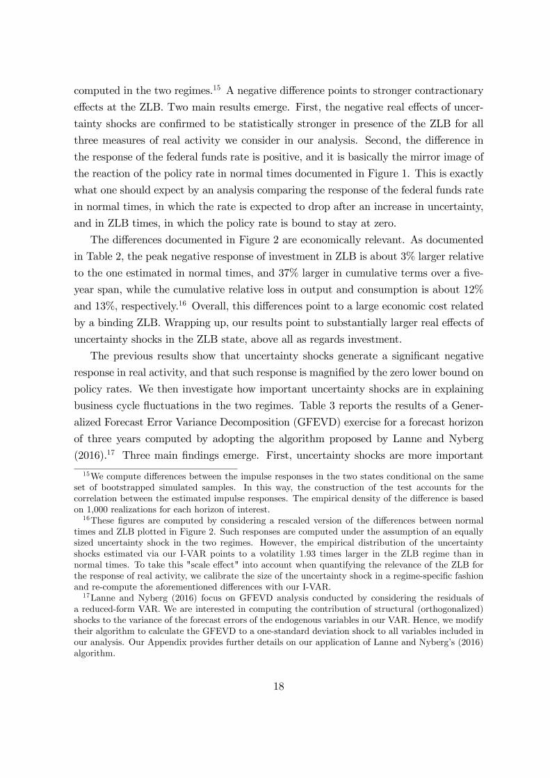
The di¤erences documented in Figure 2 are economically relevant. As documented

in Table 2, the peak negative response of investment in ZLB is about 3% larger relative

to the one estimated in normal times, and 37% larger in cumulative terms over a �ve-

year span, while the cumulative relative loss in output and consumption is about 12%

and 13%, respectively.16 Overall, this di¤erences point to a large economic cost related

by a binding ZLB. Wrapping up, our results point to substantially larger real e¤ects of

uncertainty shocks in the ZLB state, above all as regards investment.

The previous results show that uncertainty shocks generate a signi�cant negative

response in real activity, and that such response is magni�ed by the zero lower bound on

policy rates. We then investigate how important uncertainty shocks are in explaining

business cycle �uctuations in the two regimes. Table 3 reports the results of a Gener-

alized Forecast Error Variance Decomposition (GFEVD) exercise for a forecast horizon

of three years computed by adopting the algorithm proposed by Lanne and Nyberg

(2016).17 Three main �ndings emerge. First, uncertainty shocks are more important

15We compute di¤erences between the impulse responses in the two states conditional on the sameset of bootstrapped simulated samples. In this way, the construction of the test accounts for thecorrelation between the estimated impulse responses. The empirical density of the di¤erence is basedon 1,000 realizations for each horizon of interest.16These �gures are computed by considering a rescaled version of the di¤erences between normal

times and ZLB plotted in Figure 2. Such responses are computed under the assumption of an equallysized uncertainty shock in the two regimes. However, the empirical distribution of the uncertaintyshocks estimated via our I-VAR points to a volatility 1.93 times larger in the ZLB regime than innormal times. To take this "scale e¤ect" into account when quantifying the relevance of the ZLB forthe response of real activity, we calibrate the size of the uncertainty shock in a regime-speci�c fashionand re-compute the aforementioned di¤erences with our I-VAR.17Lanne and Nyberg (2016) focus on GFEVD analysis conducted by considering the residuals of

a reduced-form VAR. We are interested in computing the contribution of structural (orthogonalized)shocks to the variance of the forecast errors of the endogenous variables in our VAR. Hence, we modifytheir algorithm to calculate the GFEVD to a one-standard deviation shock to all variables included inour analysis. Our Appendix provides further details on our application of Lanne and Nyberg�s (2016)algorithm.

18

when the economy is at the ZLB. The contribution of uncertainty shocks is estimated

to be 12%, 16%, and 13% for the volatility of real GDP, investment, and consumption,

respectively. In normal times, these shares drop to 8%, 12%, and 6%. Second, uncer-

tainty shocks are relatively more important for investment than for consumption and

output. Third, the forecast error variance of the VIX is largely explained by its own

shock in both regimes (85% in normal times and 83% at the ZLB, respectively).18 All

these results are in line with the predictions o¤ered by the theoretical model by Basu

and Bundick (2016).

4.2 Robustness checks

We check the solidity of our results to a number of perturbations of the baseline I-VAR

model. In particular, we focus on i) di¤erent measures of uncertainty and identi�cation

schemes; ii) omitted variables. We present our checks below.

Alternative measures of uncertainty/ordering. Our baseline VAR models theVIX as a measure of uncertainty and puts it before real activity indicators in our vec-

tor. This way of modeling uncertainty is common in the literature (see, e.g., Bloom

(2009), Caggiano, Castelnuovo, and Groshenny (2014), Leduc and Liu (2016)). More-

over, it is in line with the theoretical model by Basu and Bundick (2016), who show

that �rst-moment or non-uncertainty shocks in their framework have almost no e¤ect

on the expected volatility of stock market returns. However, a recent contribution by

Ludvigson, Ma, and Ng (2016) closely follows the data-rich, factor-approach modelling

strategy proposed by Jurado, Ludvigson, and Ng (2015) to construct a �nancial un-

certainty index via the computation of the common component of the volatility of the

forecast errors of 147 �nancial series. Variations in this index are found to: i) sig-

ni�cantly a¤ect various real activity indicators; ii) be driven by their own "shocks".

Hence, this index is likely to carry relevant information on exogenous changes in �nan-

cial uncertainty. We then replace the VIX with the LMN �nancial uncertainty index

and re-run our estimates to check the robustness of our impulse responses.

As regards the ordering of the variables, it is of interest to check if our results

are robust to placing uncertainty last in our vector. In this way, we maximize the

contribution of non-uncertainty shocks to the volatility of the uncertainty proxy and,

therefore, challenge the role of uncertainty shocks as a driver of the business cycle. We

18Interestingly, these numbers remain mostly unchanged if the VIX is ordered last. In such a case,the volatility of the VIX is explained by its own shock for a fraction of 81.5% and 80% in the tworegimes, respectively.

19

then run exercises in which we order either the VIX or the LMN index last in our vector.

Figure 3 collects the impulse responses of our real activity indicators when the

economy is at the ZLB and in Normal times conditional on having i) the VIX ordered

�rst in the vector (baseline scenario); ii) the VIX ordered last in the vector; iii) the LMN

index ordered �rst; iv) the LMN index ordered last. The shapes and magnitudes of

these responses are very similar across these four cases. Figure 4 reports the di¤erences

between the impulse responses in the two regimes. To ease comparison with our baseline

analysis, Figure 4 reports the di¤erence between the GIRFs in the two regimes and the

68% con�dence bands estimated with our baseline vector along with the di¤erences

between the GIRFs for the other three cases we consider. The di¤erences across the

four models are quantitatively very similar. This is especially true for investment, for

which all di¤erences are included in the 68% con�dence bands estimated for our baseline

speci�cation at all horizons.

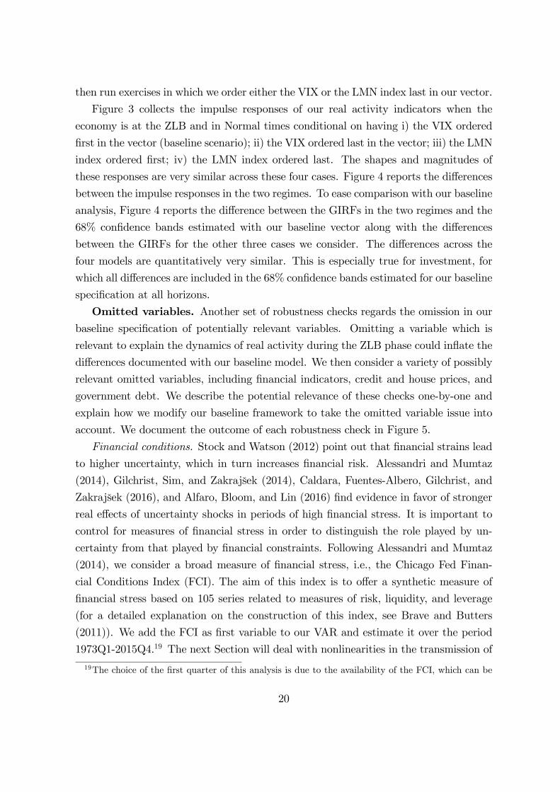
Omitted variables. Another set of robustness checks regards the omission in ourbaseline speci�cation of potentially relevant variables. Omitting a variable which is

relevant to explain the dynamics of real activity during the ZLB phase could in�ate the

di¤erences documented with our baseline model. We then consider a variety of possibly

relevant omitted variables, including �nancial indicators, credit and house prices, and

government debt. We describe the potential relevance of these checks one-by-one and

explain how we modify our baseline framework to take the omitted variable issue into

account. We document the outcome of each robustness check in Figure 5.

Financial conditions. Stock and Watson (2012) point out that �nancial strains lead

to higher uncertainty, which in turn increases �nancial risk. Alessandri and Mumtaz

(2014), Gilchrist, Sim, and Zakraj�ek (2014), Caldara, Fuentes-Albero, Gilchrist, and

Zakraj�ek (2016), and Alfaro, Bloom, and Lin (2016) �nd evidence in favor of stronger

real e¤ects of uncertainty shocks in periods of high �nancial stress. It is important to

control for measures of �nancial stress in order to distinguish the role played by un-

certainty from that played by �nancial constraints. Following Alessandri and Mumtaz

(2014), we consider a broad measure of �nancial stress, i.e., the Chicago Fed Finan-

cial Conditions Index (FCI). The aim of this index is to o¤er a synthetic measure of

�nancial stress based on 105 series related to measures of risk, liquidity, and leverage

(for a detailed explanation on the construction of this index, see Brave and Butters

(2011)). We add the FCI as �rst variable to our VAR and estimate it over the period

1973Q1-2015Q4.19 The next Section will deal with nonlinearities in the transmission of

19The choice of the �rst quarter of this analysis is due to the availability of the FCI, which can be

20

uncertainty shocks strictly related to �nancial conditions.

S&P500. The baseline speci�cation is based on the implicit hypothesis that our

VAR contains enough information to isolate second moment �nancial shocks. A way to

control for �rst moment �nancial shocks is to add a stock market index to our vector

and order it before uncertainty. Following Bloom (2009), we run an exercise in which

we add the log of S&P500 index to our VAR and order it �rst.

Credit to the non-�nancial sector. Schularik and Taylor (2012) use long time series

data and a multi-country analysis to show that credit booms are key to understand the

propagation mechanism of shocks to the real economy. Mian and Su� (2009, 2014) and

Mian, Rao, and Su� (2013) highlight the role played by credit to the private sector in

generating and prolonging the e¤ects of the Great Recession in the United States. Mian

and Su� (2014) show that the drop in employment experienced between 2007 and 2009

is likely to be due to the earlier credit boom. We then estimate a version of our VAR

in which a measure of total credit to private non-�nancial sector is ordered �rst in the

vector.20

House prices. Since Iacoviello (2005), there has been a revamped attention toward

the relationship between housing market dynamics and the business cycle. Importantly

for our exercise, Furlanetto, Ravazzolo, and Sarferaz (2014) show that the e¤ects of

uncertainty shocks are dampened if one controls for housing shocks. We then add the

log of real home price index computed by Robert Shiller as �rst variable to our vector.21

Government debt/de�cit. It is well known that monetary policy and �scal policy are

tightly connected when it comes to determining the equilibrium value of in�ation and

real activity (for an extensive presentation, see Leeper and Leigh (2016)). Christiano,

Eichenbaum, and Rebelo (2011) show that the e¤ects of expansionary �scal policy are

much larger when the economy is at the zero lower bound. The U.S. Government

implemented the stimulus package known as "American Recovery and Reinvestment

Act of 2009" in an attempt to lead the economy out of the Great Recession. We control

downloaded from the Federal Reserve Bank of St Louis�website. Unreported results (available uponrequest) show that the baseline �ndings are robust also to the inclusion of a di¤erent indicator of�nancial stress, i.e., the spread between the Baa corporate bonds and the 10-year Treasury yield.20We use the series "Total credit to private non-�nancial sector" (adjusted for breaks), which is

available on the Federal Reserve Bank of St. Louis�website. We de�ated this series with the GDPde�ator.21The index is available until 2014Q1 and it can be downloaded from here:

http://www.econ.yale.edu/~shiller/data/Fig2-1.xls . Di¤erently from house prices, oil pricesare typically associated to high in�ation in the 1970s and are considered as one of the drivers of thein�ation-output trade-o¤ in that period. An exercise (available upon request) conducted by addingoil prices to our baseline vector con�ms the solidity of our �ndings.

21

for the role of �scal policy by conducing an exercise in which the public debt-to-GDP

ratio is embedded in our vector.22

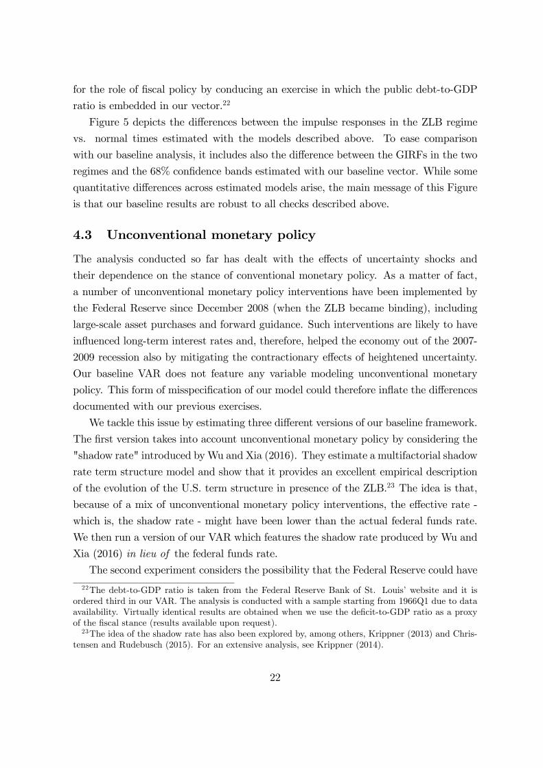
Figure 5 depicts the di¤erences between the impulse responses in the ZLB regime

vs. normal times estimated with the models described above. To ease comparison

with our baseline analysis, it includes also the di¤erence between the GIRFs in the two

regimes and the 68% con�dence bands estimated with our baseline vector. While some

quantitative di¤erences across estimated models arise, the main message of this Figure

is that our baseline results are robust to all checks described above.

4.3 Unconventional monetary policy

The analysis conducted so far has dealt with the e¤ects of uncertainty shocks and

their dependence on the stance of conventional monetary policy. As a matter of fact,

a number of unconventional monetary policy interventions have been implemented by

the Federal Reserve since December 2008 (when the ZLB became binding), including

large-scale asset purchases and forward guidance. Such interventions are likely to have

in�uenced long-term interest rates and, therefore, helped the economy out of the 2007-

2009 recession also by mitigating the contractionary e¤ects of heightened uncertainty.

Our baseline VAR does not feature any variable modeling unconventional monetary

policy. This form of misspeci�cation of our model could therefore in�ate the di¤erences

documented with our previous exercises.

We tackle this issue by estimating three di¤erent versions of our baseline framework.

The �rst version takes into account unconventional monetary policy by considering the

"shadow rate" introduced byWu and Xia (2016). They estimate a multifactorial shadow

rate term structure model and show that it provides an excellent empirical description

of the evolution of the U.S. term structure in presence of the ZLB.23 The idea is that,

because of a mix of unconventional monetary policy interventions, the e¤ective rate -

which is, the shadow rate - might have been lower than the actual federal funds rate.

We then run a version of our VAR which features the shadow rate produced by Wu and

Xia (2016) in lieu of the federal funds rate.

The second experiment considers the possibility that the Federal Reserve could have

22The debt-to-GDP ratio is taken from the Federal Reserve Bank of St. Louis�website and it isordered third in our VAR. The analysis is conducted with a sample starting from 1966Q1 due to dataavailability. Virtually identical results are obtained when we use the de�cit-to-GDP ratio as a proxyof the �scal stance (results available upon request).23The idea of the shadow rate has also been explored by, among others, Krippner (2013) and Chris-

tensen and Rudebusch (2015). For an extensive analysis, see Krippner (2014).

22

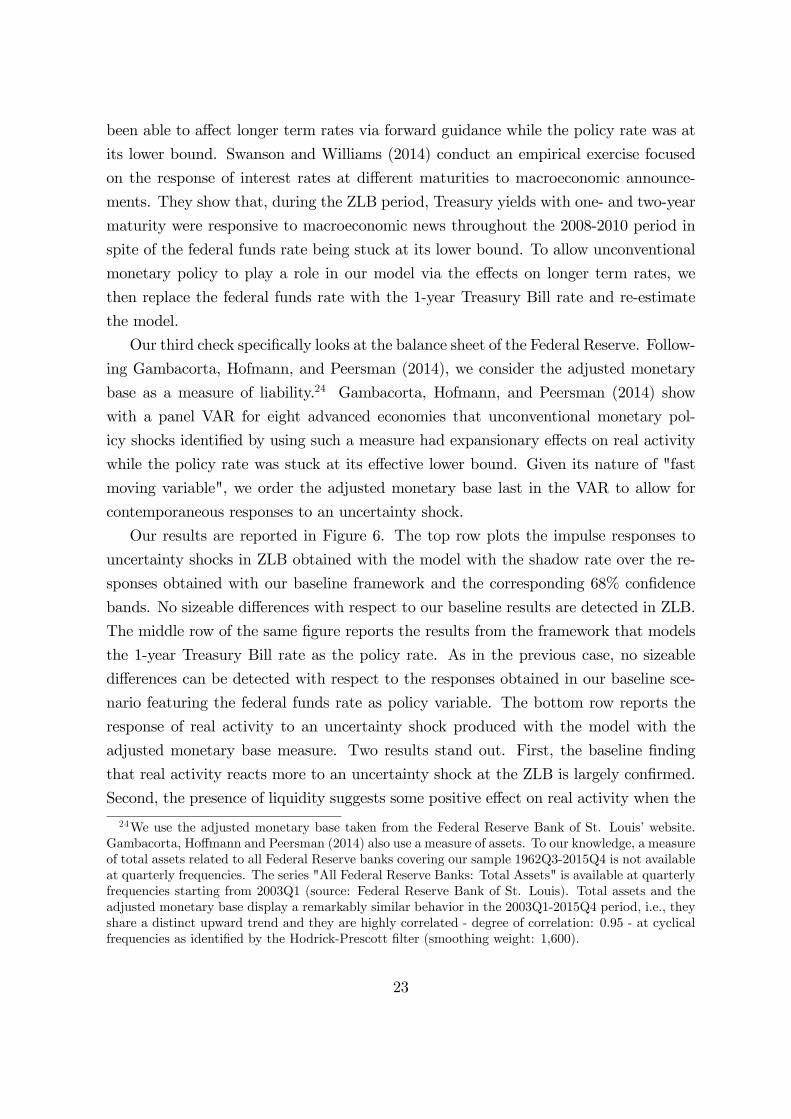
been able to a¤ect longer term rates via forward guidance while the policy rate was at

its lower bound. Swanson and Williams (2014) conduct an empirical exercise focused

on the response of interest rates at di¤erent maturities to macroeconomic announce-

ments. They show that, during the ZLB period, Treasury yields with one- and two-year

maturity were responsive to macroeconomic news throughout the 2008-2010 period in

spite of the federal funds rate being stuck at its lower bound. To allow unconventional

monetary policy to play a role in our model via the e¤ects on longer term rates, we

then replace the federal funds rate with the 1-year Treasury Bill rate and re-estimate

the model.

Our third check speci�cally looks at the balance sheet of the Federal Reserve. Follow-

ing Gambacorta, Hofmann, and Peersman (2014), we consider the adjusted monetary

base as a measure of liability.24 Gambacorta, Hofmann, and Peersman (2014) show

with a panel VAR for eight advanced economies that unconventional monetary pol-

icy shocks identi�ed by using such a measure had expansionary e¤ects on real activity

while the policy rate was stuck at its e¤ective lower bound. Given its nature of "fast

moving variable", we order the adjusted monetary base last in the VAR to allow for

contemporaneous responses to an uncertainty shock.

Our results are reported in Figure 6. The top row plots the impulse responses to

uncertainty shocks in ZLB obtained with the model with the shadow rate over the re-

sponses obtained with our baseline framework and the corresponding 68% con�dence

bands. No sizeable di¤erences with respect to our baseline results are detected in ZLB.

The middle row of the same �gure reports the results from the framework that models

the 1-year Treasury Bill rate as the policy rate. As in the previous case, no sizeable

di¤erences can be detected with respect to the responses obtained in our baseline sce-

nario featuring the federal funds rate as policy variable. The bottom row reports the

response of real activity to an uncertainty shock produced with the model with the

adjusted monetary base measure. Two results stand out. First, the baseline �nding

that real activity reacts more to an uncertainty shock at the ZLB is largely con�rmed.

Second, the presence of liquidity suggests some positive e¤ect on real activity when the

24We use the adjusted monetary base taken from the Federal Reserve Bank of St. Louis�website.Gambacorta, Ho¤mann and Peersman (2014) also use a measure of assets. To our knowledge, a measureof total assets related to all Federal Reserve banks covering our sample 1962Q3-2015Q4 is not availableat quarterly frequencies. The series "All Federal Reserve Banks: Total Assets" is available at quarterlyfrequencies starting from 2003Q1 (source: Federal Reserve Bank of St. Louis). Total assets and theadjusted monetary base display a remarkably similar behavior in the 2003Q1-2015Q4 period, i.e., theyshare a distinct upward trend and they are highly correlated - degree of correlation: 0.95 - at cyclicalfrequencies as identi�ed by the Hodrick-Prescott �lter (smoothing weight: 1,600).

23

economy is at the ZLB. In particular, relative to the baseline case, all real activity indi-

cators display a less pronounced trough and a faster recovery to the pre-shock level.25

We speculate that liquidity measures could add relevant information to models featur-

ing (o¢ cial or shadow) policy rates when it comes to quantifying the responses of real

activity to an uncertainty shock (and, possibly, to macroeconomic shocks in general).

However, these responses are statistically in line with those obtained with our baseline

model as regards the ZLB phase. Wrapping up, controlling for the shadow rate, longer

term rates, and measures of liquidity does not lead to a signi�cant change in our impulse

responses.

4.4 Time-varying GIRFs

The results we have shown so far focus on the average response of real activity to

an uncertainty shock. This is obtained by integrating out the histories (initial condi-

tions) within each regime. Given that our model is a nonlinear one, histories a¤ect the

computation of the GIRFs (Koop, Pesaran, and Potter (1996)). We then turn to the

examination of the role played by histories for our dynamic responses to an uncertainty

shock.26

Figure 7 reports three sets of results. The left column depicts the evolution of

the GIRFs to a one-standard deviation uncertainty shock for all three real activity

indicators we consider. In particular, per each given variable it plots the area identi�ed

by the maximum and minimum deviations from the trend conditional on each given

history.27 An evident within-state heterogeneity is present. In particular, looking at

normal times, the evidence of overshoot (which is, deviations from the trend which

take a positive value) changes substantially over time. The impulse responses in the

late 1970s are those with the highest overshoot realizations, while those in 2000s - well

before the ZLB - are associated with the weakest evidence of overshoot.25Unsuprisingly, the responses estimated with these three models accounting for unconventional

monetary policy display virtually no di¤erence with respect to our baseline ones in normal times, whenunconventional policies were not in place.26Histories are dated by considering the �rst lag of the VAR as the reference quarter. For instance, a

history dated 2008Q4 refers to an uncertainty shock hitting in the 2009Q1 quarter and whose impulseresponses are conditional on the values (initial conditions) for the quarters 2008Q4, 2008Q3, and2008Q2, which correspond to the three lags of our VAR.27The plots proposed in the �rst two columns of Figure 7 are bidimensional views of tridimensional

objects, i.e., the values of the impulse response of each of the three real activity indicators we con-sider along di¤erent initial conditions and horizons. These tridimensional objects are reported in ourAppendix.

24

The central column plots the GIRFs over a �ve-year horizon for every history be-

longing to the two regimes we identify (solid blue lines for normal times, dashed red

lines for the ZLB regime). The dispersion in the ZLB regime is much lower. This re-

sult is possibly due to the lower number of observations in the ZLB subsample, which

amounts to about 13% of all observations in our full sample. The mass depicted by

the bundle of GIRFs in normal times displays a wider dispersion but tends to be quite

distinct with respect to that in ZLB times. This con�rms our main �nding, i.e., the

real e¤ects of uncertainty shocks are estimated to be stronger when the economy is at

the ZLB. However, some of the responses in normal times are actually quite similar to

the responses we estimate for the ZLB period. In particular, the absence of overshoot

realizations for the histories in early 2000s - whose impulse responses are indicated with

arrows in the Figure - resembles the one we observe for the ZLB phase.

The evidence depicted in the �rst two columns of Figure 7 seems to point to an

intriguing correlation between the absence of real activity overshoot after an uncertainty

shock and histories characterized by little room to manoeuvre the policy rate. In fact,

the early 2000s were characterized by low interest rates given the response of Alan

Greenspan to the burst of the dot-com bubble, while the ZLB phase is characterized

by a policy rate close to zero due to the policy response to the �nancial crisis. The

right column of Figure 7 con�rms that this correlation is strongly present in the data.

Such column reports scatterplots constructed by considering, per each given history,

the estimated peak response of real activity against the estimated peak reduction of

the interest rate after an uncertainty shock. There is a clear relationship between the

observed overshoot dynamics in real activity and the response of conventional monetary

policy. The peak response in real activity is indeed higher in correspondence of larger

reductions in the federal funds rate in response to an exogenous hike in uncertainty.

The degree of correlation between the realizations of these two responses is as large as

-0.97 for all real activity indicators that we consider.

As anticipated in Section 4.1, Bloom�s (2009) model on heterogenous �rms along

the productivity dimension delivers a temporary medium-term overshoot caused by

the reallocation of resources from low- to high-productivity �rms after an uncertainty

shock. Our evidence suggests that lowering the interest rate is key for observing an

overshoot in real activity in our model.28 Searching for a structural interpretation, our

28The Appendix reports a related exercise. In particular, we select �ve initial histories: the begin-ning of the ZLB period, plus four other histories selected by focusing on "extreme events", i.e., weselect, within each business cycle state (recessions and expansions), the two histories associated tothe "highest" realizations of the uncertainty shocks. The contractionary e¤ects of uncertainty shocks

25

evidence can be linked to Bloom�s model as follows. First, a lower nominal interest

rate leading to a lower real rate exerts a positive in�uence on �rms�pro�ts because it

increases their present discounted value. Second, a lower real interest rate reduces �rms�

marginal costs via the downward pressure that it exerts on �rm�s rental rate of capital.

Speculatively, both these elements could facilitate the reallocation of resources from

low- to high-productivity �rms which is behind the overshoot documented in Bloom�s

(2009) model. This evidence points to a channel alternative to the ones documented

in Basu and Bundick (2016) and relative to the role played by monetary policy in the

transmission of uncertainty shocks to the real side of the economy.29

4.5 The ZLB, the Great Recession and the Great FinancialCrisis

Our I-VAR analysis aims at quantifying the e¤ects of uncertainty shocks in two di¤er-

ent regimes, normal times and the ZLB. This is the reason why our baseline framework

models an interaction term involving a measure of uncertainty and the policy rate.

However, some contributions in the literature point to nonlinearities unrelated to the

ZLB. Uncertainty shocks may exert stronger e¤ects in recessions (Caggiano, Castel-

nuovo, and Groshenny (2014), Caggiano, Castelnuovo, and Nodari (2015), Caggiano,

Castelnuovo, and Figueres (2017)). This may occur because of a lower e¤ectiveness

of monetary policy in tackling negative shocks (see, e.g., Mumtaz and Surico (2015)

and Tenreyro and Thwaites (2016)), and/or because of a stickier labor market during

downturns (Cacciatore and Ravenna (2015)). Moreover, the interaction between un-

certainty shocks and �nancial frictions may intensify during periods of high �nancial

stress (Alessandri and Mumtaz (2014), Gilchrist, Sim, and Zakraj�ek (2014), Caldara,

Fuentes-Albero, Gilchrist, and Zakraj�ek (2016)). Indeed, the 2007-2009 period was

characterized by the joint presence of the ZLB, an exceptionally severe real crisis, and

the Great Financial Crisis, which featured unprecedented levels of �nancial stress. As

a consequence, the results documented above could be assigning an exaggerated role to

the ZLB because of the omission of other channels which were contemporaneously at

are more severe when the economy is hit in quarters associated to relatively low interest rates. Thisexercise con�rms that the relevant conditioning element is the federal funds rate, and not the state ofthe business cycle.29Mumtaz and Surico (2015) and Tenreyro and Thwaites (2016) investigate the ability of a central

bank to in�uence real activity during recessions. Di¤erently, our exercise focuses on the relation-ship between the response of systematic monetary policy to an uncertainty shock and the temporaryovershoot in real activity occuring after such shock.

26

work, i.e., the business cycle channel and the �nancial cycle.

We tackle this identi�cation issue by estimating two di¤erent versions of the I-

VAR model (1)-(2). These two alternative frameworks are characterized by alternative

interaction terms which are modeled to capture the nonlinearities due to the business

cycle channel and the �nancial channel.30 Formally, we capture the role played by the

business cycle stance by estimating the following model:

yt = �+

kXj=1

Ajyt�j +

"kXj=1

cjunct�j �� lnGDPt�j

#+ ut (4)

E(utu0t) = (5)

where � lnGDPt�j � lnGDPt�j � lnGDPt�j�1 is the quarterly growth rate of GDP,which we take as a proxy of the stance of the business cycle. We estimate this model over

the sample 1962Q3-2015Q4 and compute GIRFs conditional on the ZLB period 2008Q4-

2015Q4, which is the one of interest for our discussion. If the driver of our baseline

results is not the stance of monetary policy but rather business cycle conditions, we

would expect to �nd the responses in this period to be similar to those associated to

the very same ZLB period in our baseline analysis. If, instead, such responses turn out

to be di¤erent, then our baseline impulse responses are not "observationally equivalent"

to those produced with the alternative model (4)-(5). Such evidence would lead us to

conclude that the key driver of the more recessionary responses in presence of the ZLB

is the ZLB per se, and not the contemporaneous occurrence of the Great Recession.

Notice that this exercise assumes the growth rate of real GDP to be a good proxy for

the stance of the business cycle. Chauvet (1998) and Chauvet and Piger (2008) obtain

smoothed recession probabilities for the United States from a Dynamic-Factor Markov-

Switching model applied to coincident business cycle indicators such as non-farm payroll

employment, industrial production, real personal income excluding transfer payments,

and real manufacturing and trade sales. Reassuringly, the correlation between the

growth rate of real GDP we use in this exercise and their smoothed recession probability

- available on the Federal Reserve Bank of St. Louis�website - is as large as �0:60.Figure 8 - top row reports the point estimates and the 68% con�dence bands obtained

with our baseline model as well as the GIRFs obtained with the alternative framework

(4)-(5). The responses estimated with this model and conditional on the ZLB initial

30In principle, the I-VAR could be estimated by allowing for multiple interaction terms simulta-neously. However, as anticipated in Section 3.1, the estimation of I-VARs featuring more than oneinteraction term to jointly model more than one of the channels discussed in the text failed to deliverstable models.

27

conditions are remarkably similar to those produced with the baseline model in normal

times, i.e., real activity displays a quick drop and rebound and a temporary overshoot.

Interestingly, the responses are included for all real activity indicators within the 68%

con�dence bands associated to normal times by our baseline I-VAR. This result sug-

gests that the macroeconomic dynamics documented with our baseline framework as

regards the ZLB phase are not driven by the contemporaneous occurrence of the Great

Recession.

The second check looks at the role played by �nancial stress during the ZLB period.

Alessandri and Mumtaz (2014) work with a nonlinear FAVAR framework and show

that uncertainty shocks exert stronger e¤ects in periods of high �nancial strain. The

same result is present in the empirical investigations proposed by Gilchrist, Sim, and

Zakraj�ek (2014) and Caldara, Fuentes-Albero, Gilchrist, and Zakraj�ek (2016). As

already mentioned, the ZLB period we focus on is characterized by an exceptionally

high level of �nancial stress. To take into account the possible asymmetry due to

�nancial strain, we then estimate the following I-VAR speci�cation:

yt = �+kXj=1

Ajyt�j +

"kXj=1

cjunct�j �GZt�j

#+ ut (6)

E(utu0t) = (7)

where GZt indicates the measure of credit spread proposed by Gilchrist and Zakraj�ek

(2012) (GZ henceforth). As before, we estimate this model over the sample 1962Q3-

2015Q4 and compute GIRFs by integrating over the period 2008Q4-2015Q4.31 We order

the GZ spread second in our vector to capture the e¤ect that �nancial markets are likely

to play in transmitting the impact of an uncertainty shock on the economy (Gilchrist,

Sim, and Zakraj�ek (2014), Caldara, Fuentes-Albero, Gilchrist, and Zakraj�ek (2016)).

The logic of this exercise is the same as the one in the previous exercise. If the driver

of our baseline results is not the stance of monetary policy but rather the �nancial strain,

model (6)-(7) should return impulse responses which are similar to the baseline ZLB

and di¤erent from the ones that the baseline model associates to normal times.31The original version of the GZ spread is available from 1973. Our baseline analysis starts in 1962.

Then, we regress the GZ spread against the di¤erence between i) the AAA corporate bonds and the10-year Treasury yield; ii) the BAA corporate bonds and the 10-year Treasury yield; iii) the 6-monthT-Bill rate and the 3-month T-Bill rate; iv) the 1-year Treasury yield and the 3-month T-Bill rate; v)the 10-year Treasury yield and the 3-month T-Bill rate. We do this for the sample 1973-2015, and thenwe use the �tted values of the regression to backcast the GZ spread and match our baseline sample.All data are taken from the Federal Reserve Bank of St. Louis�database.

28

Figure 8 - bottom row shows that this is not the case. In fact, if we let the interaction

between uncertainty and the GZ credit spread capture the nonlinearity of the e¤ects

of uncertainty shocks, we get a response of real activity in the ZLB sample which is

actually very similar to the one that our baseline model associates to normal times.

Noticeably, as in the previous case, the responses of all real activity measures lie within

the 68% con�dence bands estimated for normal times in the baseline I-VAR.

Our results should be seen as complementary with respect to those proposed by

papers that study the e¤ects of uncertainty shocks in good and bad times (Caggiano,

Castelnuovo, and Groshenny (2014), Caggiano, Castelnuovo, and Nodari (2015), Caggiano,

Castelnuovo, and Figueres (2017)) or in periods of high �nancial stress (Alessandri and

Mumtaz (2014), Gilchrist, Sim, and Zakraj�ek (2014), and Caldara, Fuentes-Albero,

Gilchrist, and Zakraj�ek (2016)). In fact, these papers and ours tackle di¤erent re-

search questions. Our paper explicitly deals with the ZLB, which is quite a peculiar

event in the U.S. post-WWII economic history. Hence, a correct reading of our �ndings

is that the Great Recession and the high levels of �nancial stress occurred during the

global �nancial crisis would not be enough to explain the bigger impact on real activity

documented by our impulse responses during the 2008Q4-2015Q4 period. Di¤erently,

the ZLB is able to generate signi�cantly di¤erent responses during the ZLB as opposed

to the pre-2008Q4 period. Our conclusion is that heightened uncertainty in presence of

the ZLB makes things even worse than they would be in a world in which the policy

rate is away for its bound.

Finally, a di¤erent question regards the role played by �rst moment shocks which

may have originated before the ZLB period, led the U.S. economy to the ZLB, and had

a large and negative impact during the ZLB period. In this case, such shocks could be

behind our results, and the larger response of real activity to uncertainty shocks would

not be caused by the ZLB, but simply correlated to it. We check for this possibility

by running an exercise in which we compute the GIRFs by shutting down future non-

uncertainty shocks one at a time. In conducting this exercise, we focus on shocks to

prices, output, investment, and consumption. If one of these shocks (or a combination

of them) is actually behind the results documented in the previous Section, we should

observe a drastic change in our GIRFs and, in particular, more similar responses between

regimes. The outcome of this exercise, reported in the Appendix for the sake of brevity,

con�rms that our main conclusion on the deeper recession opened by an uncertainty

shock during the ZLB regime remains una¤ected.

29

5 Conclusions

This paper works with a nonlinear Interacted-VAR framework and post-WWII U.S.

data and shows that uncertainty shocks triggered a deeper recession during the zero

lower bound period than in times of unconstrained monetary policy. This result is

shown not to be driven by other macroeconomic shocks that occurred during the Great

Recession or by the presence of more severe �nancial conditions, and it is robust to

di¤erent ways of modeling unconventional monetary policy. Our paper also documents

a clear correlation between the response of monetary policy authorities to uncertainty

shocks when the policy rate is away from the bound and the presence of a temporary

overshoot of real activity. In particular, the more aggressive the monetary policy easing,

the larger the overshoot.

From a modeling standpoint, our results support the employment of general equi-

librium frameworks i) which predict a larger response of real activity to an uncertainty

shock in presence of the ZLB, and ii) are able to generate macroeconomic comove-

ments after an uncertainty shock. Models by Johannsen (2014), Fernández-Villaverde,

Guerrón-Quintana, Kuester, and Rubio-Ramírez (2015), and Basu and Bundick (2015,

2016) are promising proposals along these lines. As regards the real activity overshoot

caused by a monetary policy shock, our results support models featuring heterogeneous

units and a real option channel as in Bloom (2009), who shows that the reallocation of

resources from low- to high-productivity �rms can be facilitated by lower factor prices.

To our knowledge, the extant literature features no model contemporaneously delivering

comovements, temporary overshoot, and a larger response of real activity to uncertainty

shocks in presence of the ZLB. We believe the combination of sticky prices and het-

erogeneous units in a model in which precautionary savings and real options play a

meaningful role to be a promising avenue for future research.

Finally, our results clearly call for studies focusing on optimal monetary policy in

presence of the ZLB when uncertainty shocks hit an economic system. Contributions

like Basu and Bundick (2015), Evans et al. (2015), and Seneca (2016) represent relevant

starting points for this research agenda.

ReferencesAastveit, K. A., G. J. Natvik, and S. Sola (2013): �Macroeconomic Uncertaintyand the E¤ectiveness of Monetary Policy,�Norges Bank Working Paper No. 2013/17.

30

Alessandri, P., and H. Mumtaz (2014): �Financial Regimes and UncertaintyShocks,�Queen Mary University of London Working Paper No. 729.

Alfaro, I., N. Bloom, and X. Lin (2016): �The Finance-Uncertainty Multiplier,�Stanford University and Ohio State University.

Aruoba, S., L. Bucola, and F. Schorfheide (2013): �Assessing DSGE ModelNonlinearities,�NBER Working Paper No. 19693.

Baker, S., N. Bloom, and S. J. Davis (2016): �Measuring Economic Policy Uncer-tainty,�Quarterly Journal of Economics, 131(4), 1539�1636.

Basu, S., and B. Bundick (2015): �Endogenous Volatility at the Zero Lower Bound:Implications for Stabilization Policy,�Federal Reserve Bank of Kansas City ResearchWorking Paper No. 15-01.

(2016): �Uncertainty Shocks in a Model of E¤ective Demand,�Econometrica,forthcoming.

Bekaert, G., M. Hoerova, and M. Lo Duca (2013): �Risk, Uncertainty andMonetary Policy,�Journal of Monetary Economics, 60, 771�788.

Bianchi, F., and L. Melosi (2017): �Escaping the Great Recession,� AmericanEconomic Review, forthcoming.

Bloom, N. (2009): �The Impact of Uncertainty Shocks,�Econometrica, 77(3), 623�685.

(2014): �Fluctuations in Uncertainty,� Journal of Economic Perspectives,28(2), 153�176.

Born, B., and J. Pfeifer (2015): �Uncertainty-driven business cycles: assessing themarkup channel,�University of Bonn, mimeo.

Brave, S., and R. A. Butters (2011): �Monitoring Financial Stability: A FinancialConditions Index Approach,�Federal Reserve Bank of Chicago Economic Perspec-tives 1Q/2011.

Cacciatore, M., and F. Ravenna (2015): �Uncertainty, Wages, and the BusinessCycle,�HEC Montreal, mimeo.

Caggiano, G., E. Castelnuovo, and J. M. Figueres (2017): �Economic Pol-icy Uncertainty and Unemployment in the United States: A Nonlinear Approach,�Economics Letters, 151, 31�34.

Caggiano, G., E. Castelnuovo, and N. Groshenny (2014): �Uncertainty Shocksand Unemployment Dynamics: An Analysis of Post-WWII U.S. Recessions,�Journalof Monetary Economics, 67, 78�92.

Caggiano, G., E. Castelnuovo, and G. Nodari (2015): �Uncertainty and Mon-etary Policy in Good and Bad Times,�University of Padova and University of Mel-bourne, mimeo.

Caldara, D., C. Fuentes-Albero, S. Gilchrist, and E. Zakraj�ek (2016):�The Macroeconomic Impact of Financial and Uncertainty shocks,�European Eco-nomic Review, forthcoming.

31

Chan, J. C., and R. Strachan (2014): �The Zero Lower Bound: Implicationsfor Modelling the Interest Rate,�Australian National University and University ofQueensland, mimeo.

Chauvet, M. (1998): �An Economic Characterization of Business Cycle Dynamicswith Factor Structure and Regime Switching,� International Economic Review, 39,969�996.

Chauvet, M., and J. Piger (2008): �A Comparison of the Real-Time Performanceof Business Cycle Dating Methods,� Journal of Business and Economic Statistics,26, 42�49.

Christensen, J., and G. D. Rudebusch (2015): �Estimating shadow-rate termstructure models with near-zero yields,� Journal of Financial Econometrics, 13(2),226�259.

Christiano, L. J., M. Eichenbaum, and S. Rebelo (2011): �When is the Govern-ment Spending Multiplier Large?,�Journal of Political Economy, 119(1), 78�121.

Evans, C., J. D. M. Fisher, F. Gourio, and S. Krane (2015): �Risk Managementfor Monetary Policy Near the Zero Lower Bound,�Brookings Papers on EconomicActivity, forthcoming.

Fernández-Villaverde, J., P. Guerrón-Quintana, K. Kuester, and J. F.Rubio-Ramírez (2015): �Fiscal Volatility Shocks and Economic Activity,�Ameri-can Economic Review, 105(11), 3352�3384.

Furlanetto, F., F. Ravazzolo, and S. Sarferaz (2014): �Identi�cation of �nan-cial factors in economic �uctuations,�Norges Bank Working Paper No. 09/2014.

Gambacorta, L., B. Hofmann, and G. Peersman (2014): �The E¤ectiveness ofUnconventional Monetary Policy at the Zero Lower Bound: A Cross-Country Analy-sis,�Journal of Money, Credit and Banking, 46(4), 615�642.

Gilchrist, S., J. W. Sim, and E. Zakraj�ek (2014): �Uncertainty, Financial Fric-tions, and Investment Dynamics,�Boston University and Federal Reserve Board ofGovernors, mimeo.

Gilchrist, S., and E. Zakraj�ek (2012): �Credit Spreads and Business Cycle Fluc-tuations,�American Economic Review, 102(4), 1692�1720.

Granger, C. W. (1998): �Overview of Nonlinear Time Series Speci�cation in Eco-nomics,�University of California, San Diego.

Iacoviello, M. (2005): �House Prices, Borrowing Constraints and Monetary Policyin the Business Cycle,�American Economic Review, 95(3), 739�764.

Johannsen, B. K. (2014): �When are the E¤ects of Fiscal Policy Uncertainty Large?,�Board of Governors of the Federal Reserve System, Finance and Economics DiscussionSeries 2014-40.

Jurado, K., S. C. Ludvigson, and S. Ng (2015): �Measuring Uncertainty,�Amer-ican Economic Review, 105(3), 1177�1216.

32

Kilian, L., and R. Vigfusson (2011): �Are the Responses of the U.S. EconomyAsymmetric in Energy Price Increases and Decreases?,�Quantitative Economics, 2,419�453.

Koop, G., M. Pesaran, and S. Potter (1996): �Impulse response analysis innonlinear multivariate models,�Journal of Econometrics, 74(1), 119�147.

Krippner, L. (2013): �Measuring the stance of monetary policy in zero lower boundenvironments,�Economics Letters, 118(1), 135�138.

(2014): Term Structure Modeling at the Zero Lower Bound: A Practitioner�sGuide, Palgrave-Macmillan, forthcoming.

Lanne, M., and H. Nyberg (2016): �Generalised Forecast Error Variance Decompo-sition for Linear and Nonlinear Multivariate Models,�Oxford Bulletin of Economicsand Statistics, 78, 595�603.

Leduc, S., and Z. Liu (2016): �Uncertainty Shocks are Aggregate Demand Shocks,�Journal of Monetary Economics, 82, 20�35.

Leeper, E. (1991): �Equilibria Under �Active� and �Passive�Monetary and FiscalPolicies,�Journal of Monetary Economics, 27, 129�147.

Leeper, E. M., and C. Leigh (2016): �Understanding In�ation as a Joint Monetary-Fiscal Phenomenon,� in: J.B. Taylor and H. Uhlig (eds.): Handbook of Macroeco-nomics, Elsevier Science, forthcoming.

Ludvigson, S. C., S. Ma, and S. Ng (2016): �Uncertainty and Business Cycles:Exogenous Impulse or Endogenous Response?,�New York University and ColumbiaUniversity, mimeo.

Mian, A., K. Rao, and A. Sufi (2013): �Household Balance Sheet, Consumption,and the Economic Slump,�Quarterly Journal of Economics, 128(4), 1687�1726.

Mian, A., and A. Sufi (2009): �The Consequences of Mortgage Credit Expansion:Evidence from the U.S. Mortgage Default Crisis,�Quarterly Journal of Economics,124(4), 1449�1496.

(2014): �What Explains the 2007-2009 Drop in Employment?,�Econometrica,82(6), 2197�2223.

Mittnik, S. (1990): �Modeling Nonlinear Processes With Generalized Autoregres-sions,�Applied Mathematics Letters, 3(4), 71�74.

Mumtaz, H., and P. Surico (2015): �The Transmission Mechanism in Good andBad Times,�International Economic Review, 56, 1237�1260.

Nakata, T. (2016): �Uncertainty at the Zero Lower Bound,� American EconomicJournal: Macroeconomics, forthcoming.

Nodari, G. (2014): �Financial Regulation Policy Uncertainty and Credit Spreads inthe U.S.,�Journal of Macroeconomics, 41, 122�132.

Pellegrino, G. (2014): �Uncertainty and Monetary Policy in the US: A Journeyinto Non-Linear Territory,�University of Padova "Marco Fanno" Working Paper No.184-2014.

33

Plante, M., A. W. Richter, and N. A. Throckmorton (2016): �The Zero LowerBound and Endogenous Uncertainty,�Economic Journal, forthcoming.

Ramey, V. A., and S. Zubairy (2016): �Government Spending Multipliers in GoodTimes and in Bad: Evidence from U.S. Historical Data,�Journal of Political Econ-omy, forthcoming.

Rossi, B., and T. Sekhposyan (2015): �Macroeconomic Uncertainty Indices Basedon Nowcast and Forecast Error Distributions,�American Economic Review Papersand Proceedings, 105(5), 650�655.

Ruge-Murcia, F. (2015): �Indirect Inference Estimation of Nonlinear Dynamic Gen-eral EquilibriumModels: With an Application to Asset Pricing under Skewness Risk,�McGill University, mimeo.

Schularik, M., and A. M. Taylor (2012): �Credit Booms Gone Bust: MonetaryPolicy, Leverage Cycles, and Financial Crises, 1870-2008,�American Economic Re-view, 102(2), 1029�1061.

Seneca, M. (2016): �Risk Shocks Close to the Zero Lower Bound,�Bank of EnglandSta¤Working Paper No. 606.

Stock, J. H., and M. W. Watson (2012): �Disentangling the Channels of the 2007-2009 Recession,�Brookings Papers on Economic Activity, Spring, 81�135.

Sá, F., P. Towbin, and T. Wieladek (2014): �Capital In�ows, Financial Structureand Housing Booms,�Journal of the European Economic Association, 12(2), 522�546.

Tenreyro, S., and G. Thwaites (2016): �Pushing on a string: US monetary pol-icy is less powerful in recessions,� American Economic Journal: Macroeconomics,forthcoming.

Towbin, P., and S. Weber (2013): �Limits of �oating exchange rates: The roleof foreign currency debt and import structure,�Journal of Development Economics,101(1), 179�101.

Wu, J. C., and F. D. Xia (2016): �Measuring the Macroeconomic Impact of MonetaryPolicy at the Zero Lower Bound,�Journal of Money, Credit, and Banking, 48(2-3),253�291.

34

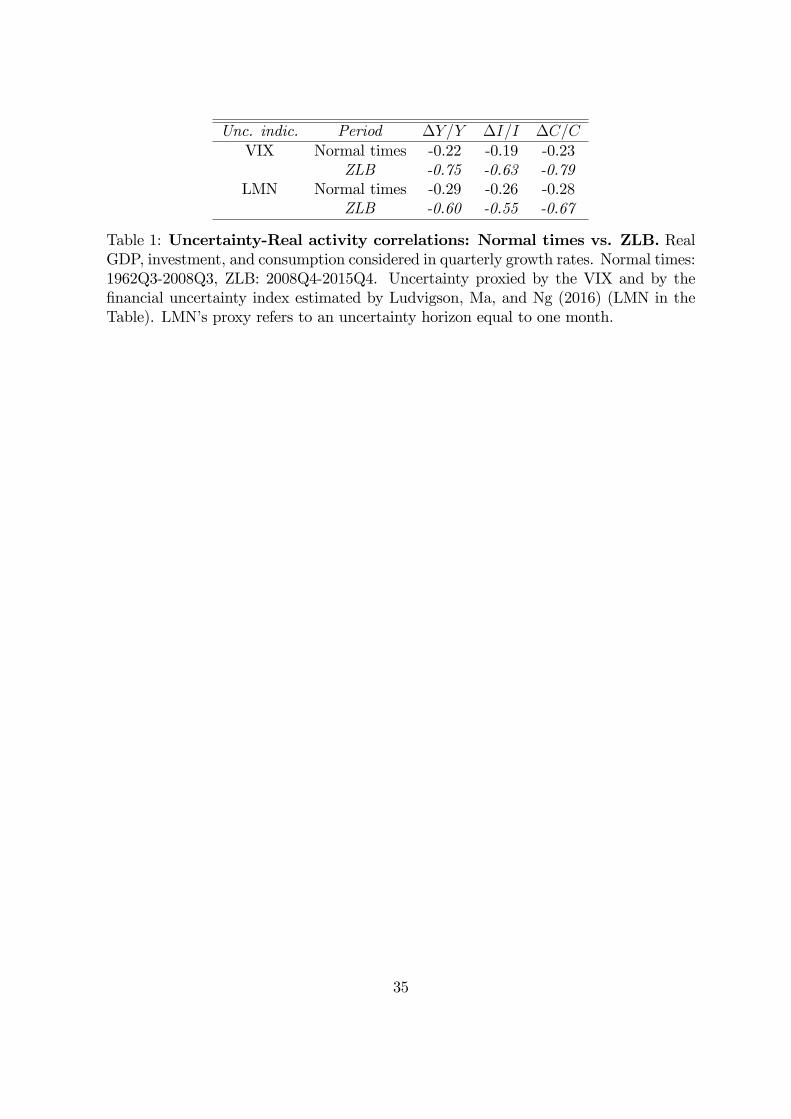
Unc. indic. Period �Y=Y �I=I �C=CVIX Normal times -0.22 -0.19 -0.23

ZLB -0.75 -0.63 -0.79LMN Normal times -0.29 -0.26 -0.28

ZLB -0.60 -0.55 -0.67

Table 1: Uncertainty-Real activity correlations: Normal times vs. ZLB. RealGDP, investment, and consumption considered in quarterly growth rates. Normal times:1962Q3-2008Q3, ZLB: 2008Q4-2015Q4. Uncertainty proxied by the VIX and by the�nancial uncertainty index estimated by Ludvigson, Ma, and Ng (2016) (LMN in theTable). LMN�s proxy refers to an uncertainty horizon equal to one month.

35

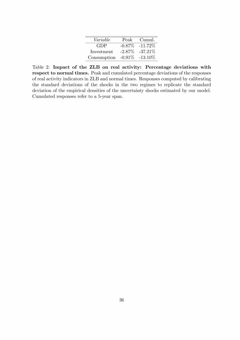
Variable Peak Cumul.GDP -0.87% -11.72%

Investment -2.87% -37.21%Consumption -0.91% -13.10%

Table 2: Impact of the ZLB on real activity: Percentage deviations withrespect to normal times. Peak and cumulated percentage deviations of the responsesof real activity indicators in ZLB and normal times. Responses computed by calibratingthe standard deviations of the shocks in the two regimes to replicate the standarddeviation of the empirical densities of the uncertainty shocks estimated by our model.Cumulated responses refer to a 5-year span.

36

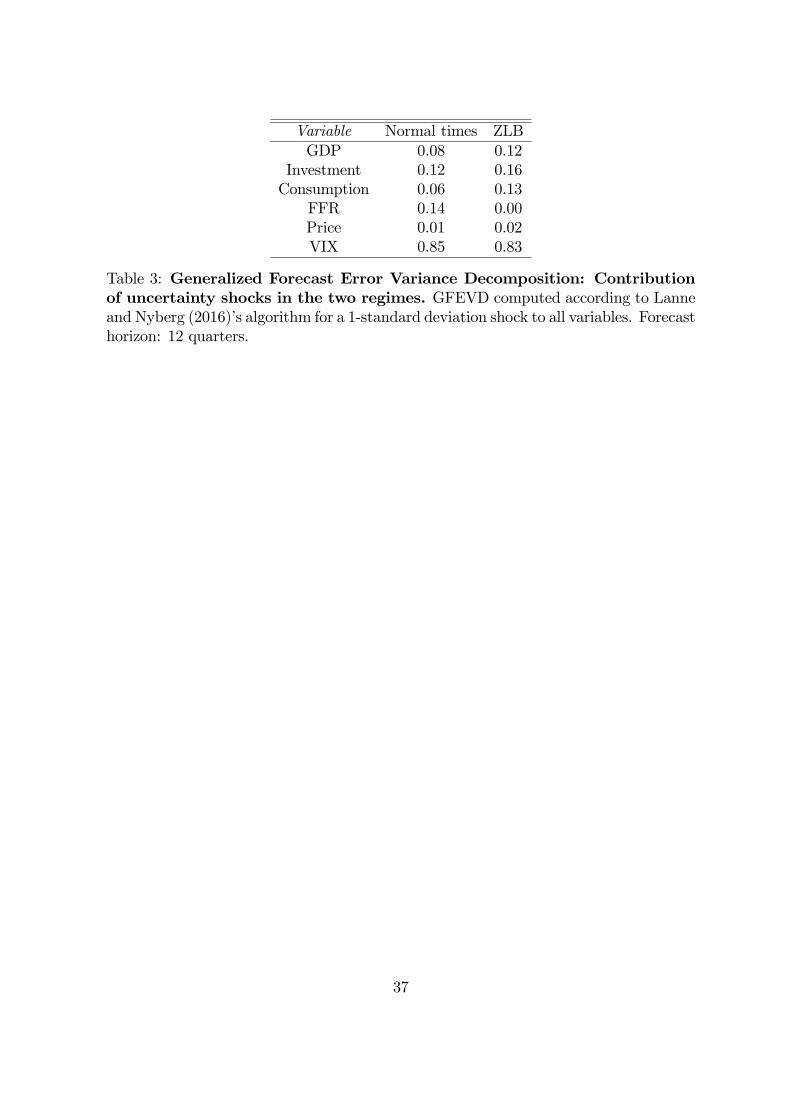
Variable Normal times ZLBGDP 0.08 0.12

Investment 0.12 0.16Consumption 0.06 0.13

FFR 0.14 0.00Price 0.01 0.02VIX 0.85 0.83

Table 3: Generalized Forecast Error Variance Decomposition: Contributionof uncertainty shocks in the two regimes. GFEVD computed according to Lanneand Nyberg (2016)�s algorithm for a 1-standard deviation shock to all variables. Forecasthorizon: 12 quarters.

37

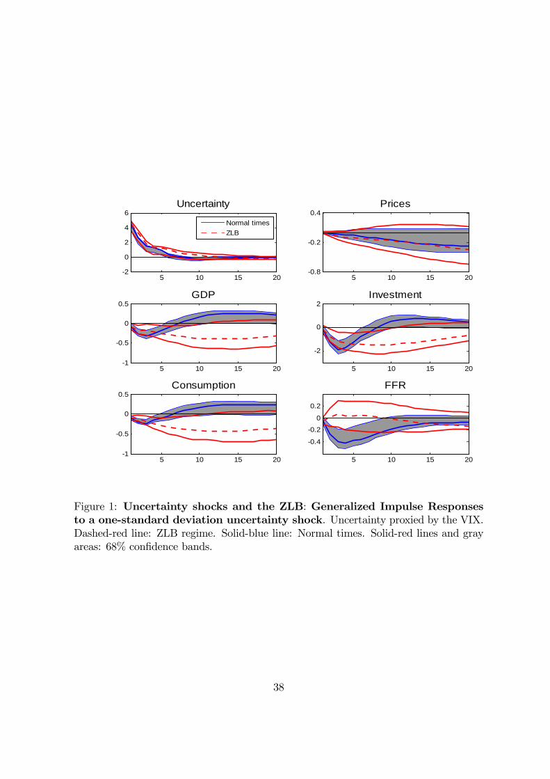
Uncertainty

5 10 15 20­2

0

2

4

6Normal timesZLB

Prices

5 10 15 20­0.8

­0.2

0.4

GDP

5 10 15 20­1

­0.5

0

0.5Investment

5 10 15 20

­2

0

2

Consumption

5 10 15 20­1

­0.5

0

0.5FFR

5 10 15 20

­0.4

­0.20

0.2

Figure 1: Uncertainty shocks and the ZLB: Generalized Impulse Responsesto a one-standard deviation uncertainty shock. Uncertainty proxied by the VIX.Dashed-red line: ZLB regime. Solid-blue line: Normal times. Solid-red lines and grayareas: 68% con�dence bands.

38

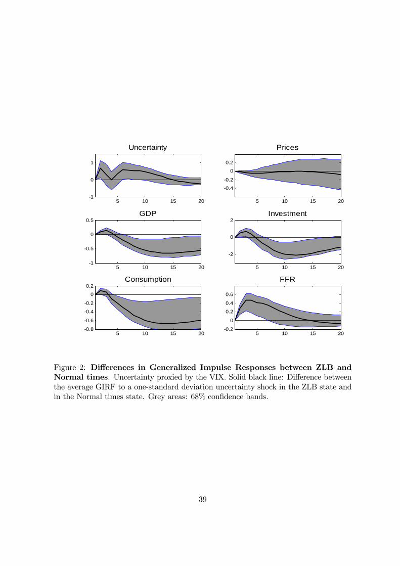
Uncertainty

5 10 15 20­1

0

1

Prices

5 10 15 20

­0.4­0.2

00.2

GDP

5 10 15 20­1

­0.5

0

0.5Investment

5 10 15 20

­2

0

2

Consumption

5 10 15 20­0.8

­0.6

­0.4­0.2

00.2

FFR

5 10 15 20­0.2

0

0.20.4

0.6

Figure 2: Di¤erences in Generalized Impulse Responses between ZLB andNormal times. Uncertainty proxied by the VIX. Solid black line: Di¤erence betweenthe average GIRF to a one-standard deviation uncertainty shock in the ZLB state andin the Normal times state. Grey areas: 68% con�dence bands.

39

VIX 

­ bas

elin

e GDP

5 10 15 20­1

­0.5

0

0.5Investment

5 10 15 20­4

­2

0

2Consumption

5 10 15 20­1

­0.5

0

0.5

Normal timesZLB

VIX 

last

5 10 15 20­1

­0.5

0

0.5

5 10 15 20­2

0

2

5 10 15 20­1

­0.5

0

0.5

LMN 

first

5 10 15 20­1

­0.5

0

0.5

5 10 15 20­4

­2

0

2

5 10 15 20­1

­0.5

0

0.5

LMN

 last

5 10 15 20­0.5

0

0.5

5 10 15 20­2

0

2

5 10 15 20­0.5

0

0.5

Figure 3: Uncertainty shocks and the ZLB: Alternative measures/orderingof uncertainty. GIRFs to a one-standard deviation uncertainty shock. Proxies ofuncertainty: VIX and LMN (measure proposed by Ludvigson, Ma and Ng (2016)).Row 1: VIX ordered �rst. Row 2: VIX ordered last. Row 3: LMN ordered �rst. Row4: LMN ordered last.

40

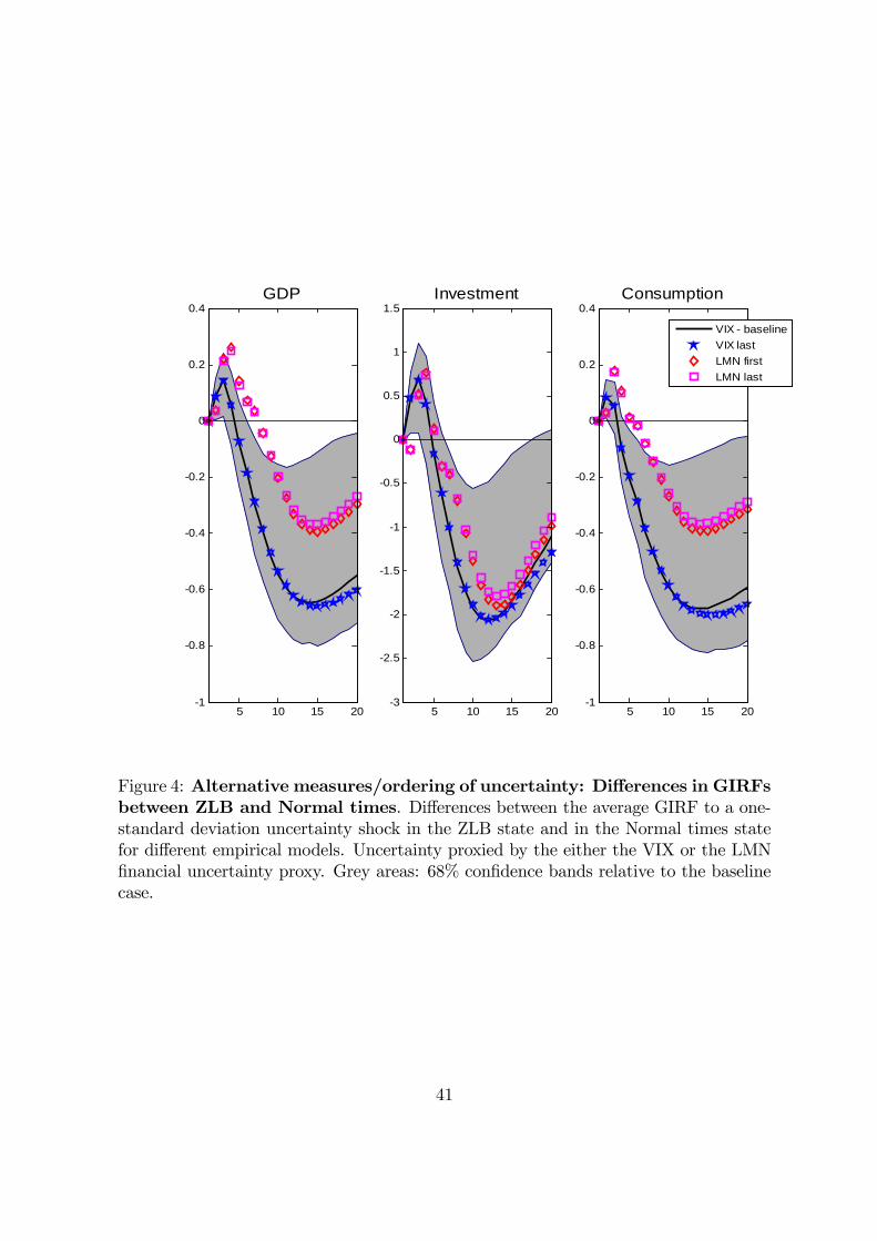
GDP

5 10 15 20­1

­0.8

­0.6

­0.4

­0.2

0

0.2

0.4Investment

5 10 15 20­3

­2.5

­2

­1.5

­1

­0.5

0

0.5

1

1.5Consumption

5 10 15 20­1

­0.8

­0.6

­0.4

­0.2

0

0.2

0.4

VIX ­ baselineVIX lastLMN firstLMN last

Figure 4: Alternative measures/ordering of uncertainty: Di¤erences in GIRFsbetween ZLB and Normal times. Di¤erences between the average GIRF to a one-standard deviation uncertainty shock in the ZLB state and in the Normal times statefor di¤erent empirical models. Uncertainty proxied by the either the VIX or the LMN�nancial uncertainty proxy. Grey areas: 68% con�dence bands relative to the baselinecase.

41

GDP

5 10 15 20­1

­0.8

­0.6

­0.4

­0.2

0

0.2

0.4Investment

5 10 15 20­3

­2.5

­2

­1.5

­1

­0.5

0

0.5

1

1.5Consumption

5 10 15 20­1

­0.8

­0.6

­0.4

­0.2

0

0.2

0.4BaselineFCISP500CreditHouse pr.B/Y

Figure 5: Uncertainty shocks and the ZLB: Di¤erences: Robustness checks.Di¤erences between the average GIRF to a one-standard deviation uncertainty shock inthe ZLB state and in the Normal times state for di¤erent empirical models. Uncertaintyproxied by the VIX. Grey areas: 68% con�dence bands relative to the baseline case.

42

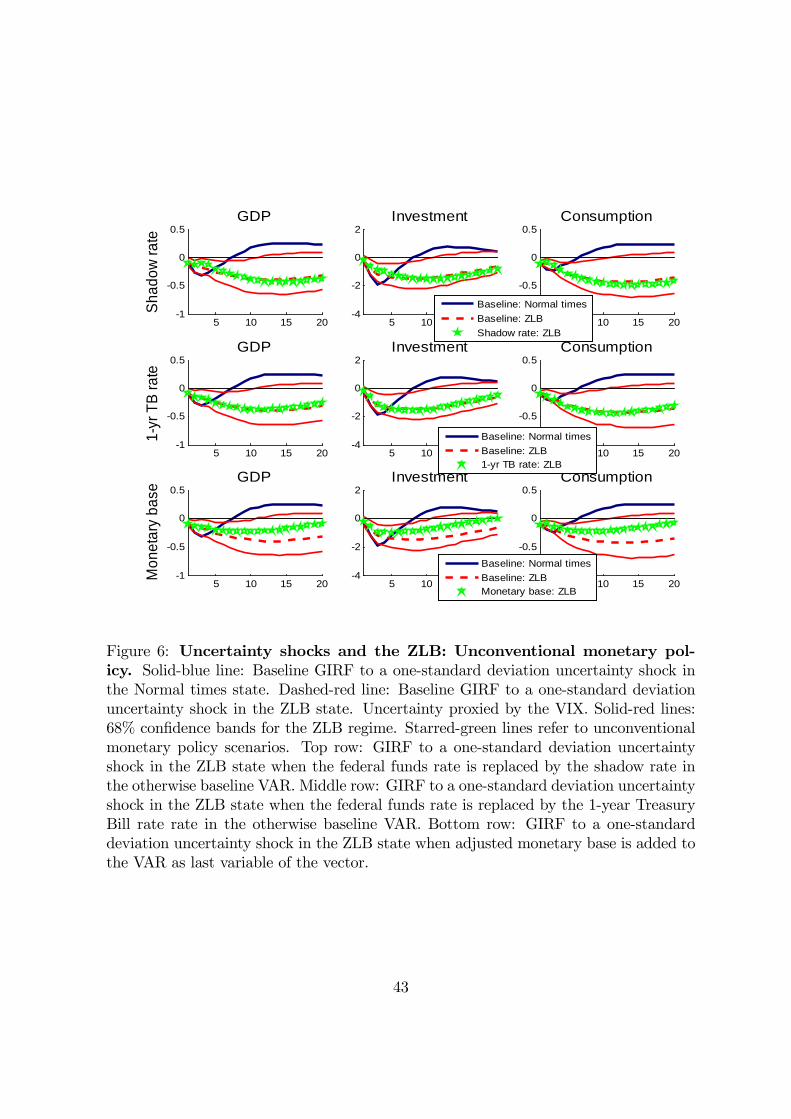
5 10 15 20­1

­0.5

0

0.5GDP

Mon

etar

y ba

se

5 10 15 20­4

­2

0

2Investment

5 10 15 20­1

­0.5

0

0.5Consumption

Baseline: Normal timesBaseline: ZLBMonetary base: ZLB

5 10 15 20­1

­0.5

0

0.5

Shad

ow ra

te

GDP

5 10 15 20­4

­2

0

2Investment

5 10 15 20­1

­0.5

0

0.5Consumption

Baseline: Normal timesBaseline: ZLBShadow rate: ZLB

5 10 15 20­1

­0.5

0

0.5

1­yr

 TB 

rate

GDP

5 10 15 20­4

­2

0

2Investment

5 10 15 20­1

­0.5

0

0.5Consumption

Baseline: Normal timesBaseline: ZLB1­yr TB rate: ZLB

Figure 6: Uncertainty shocks and the ZLB: Unconventional monetary pol-icy. Solid-blue line: Baseline GIRF to a one-standard deviation uncertainty shock inthe Normal times state. Dashed-red line: Baseline GIRF to a one-standard deviationuncertainty shock in the ZLB state. Uncertainty proxied by the VIX. Solid-red lines:68% con�dence bands for the ZLB regime. Starred-green lines refer to unconventionalmonetary policy scenarios. Top row: GIRF to a one-standard deviation uncertaintyshock in the ZLB state when the federal funds rate is replaced by the shadow rate inthe otherwise baseline VAR. Middle row: GIRF to a one-standard deviation uncertaintyshock in the ZLB state when the federal funds rate is replaced by the 1-year TreasuryBill rate rate in the otherwise baseline VAR. Bottom row: GIRF to a one-standarddeviation uncertainty shock in the ZLB state when adjusted monetary base is added tothe VAR as last variable of the vector.

43

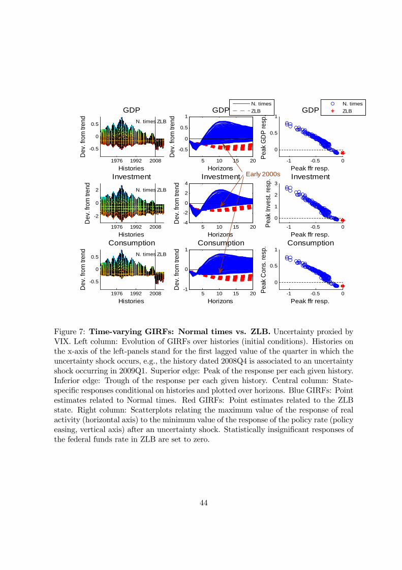
5 10 15 20

­0.5

0

0.5

1

HorizonsD

ev. f

rom

 tren

d

GDPN. timesZLB

5 10 15 20­4

­2

0

2

4Investment

Horizons

Dev

. fro

m tr

end

5 10 15 20­1

0

1Consumption

Horizons

Dev

. fro

m tr

end

1976 1992 2008

­0.5

0

0.5 ZLBN. times

GDP

Histories

Dev

. fro

m tr

end

1976 1992 2008

­2

0

2 ZLBN. times

Investment

Histories

Dev

. fro

m tr

end

1976 1992 2008

­0.5

0

0.5 ZLBN. times

Consumption

Histories

Dev

. fro

m tr

end

­1 ­0.5 0

0

0.5

1

Peak ffr resp.

Peak

 GD

P re

sp. GDP

N. timesZLB

­1 ­0.5 0

0

1

2

3

Peak ffr resp.

Peak

 Inve

st. r

esp.

Investment

­1 ­0.5 0

0

0.5

1

Peak ffr resp.

Peak

 Con

s. re

sp. Consumption

Early 2000s

Figure 7: Time-varying GIRFs: Normal times vs. ZLB. Uncertainty proxied byVIX. Left column: Evolution of GIRFs over histories (initial conditions). Histories onthe x-axis of the left-panels stand for the �rst lagged value of the quarter in which theuncertainty shock occurs, e.g., the history dated 2008Q4 is associated to an uncertaintyshock occurring in 2009Q1. Superior edge: Peak of the response per each given history.Inferior edge: Trough of the response per each given history. Central column: State-speci�c responses conditional on histories and plotted over horizons. Blue GIRFs: Pointestimates related to Normal times. Red GIRFs: Point estimates related to the ZLBstate. Right column: Scatterplots relating the maximum value of the response of realactivity (horizontal axis) to the minimum value of the response of the policy rate (policyeasing, vertical axis) after an uncertainty shock. Statistically insigni�cant responses ofthe federal funds rate in ZLB are set to zero.

44

GDP

Inte

ract

ion 

with

 GDP

5 10 15 20­0.4

­0.2

0

0.2

0.4Investment

5 10 15 20­3

­2

­1

0

1

2Consumption

5 10 15 20­0.6

­0.4

­0.2

0

0.2

0.4

Baseline: Normal timesBaseline: ZLBInteraction with GDP g.r.: ZLB

GDP

Inte

ract

ion 

with

 GZ 

spre

ad

5 10 15 20­0.4

­0.2

0

0.2

0.4Investment

5 10 15 20­3

­2

­1

0

1

2Consumption

5 10 15 20­0.6

­0.4

­0.2

0

0.2

0.4

Baseline: Normal timesBaseline: ZLBInteraction with GZ spread: ZLB

Figure 8: Uncertainty shocks during the ZLB period: Role of the businesscycle and �nancial frictions. GIRFs to a one-standard deviation uncertainty shockin the ZLB state and in the Normal times state according to our baseline model andto models featuring alternative interaction terms. Solid-blue line: Baseline GIRF toa one-standard deviation uncertainty shock in the Normal times state. Dashed-redline: Baseline GIRF to a one-standard deviation uncertainty shock in the ZLB state.Starred-magenta lines refer to models featuring alternative interaction terms. Top row:Interaction terms involving uncertainty and real GDP growth rate. Bottom row: Inter-action terms involving uncertainty and the GZ spread. Grey areas and solid-red lines:68% con�dence bands relative to the baseline case. Uncertainty proxied by the VIX.

45

Appendix of the paper "Estimating the Real E¤ectsof Uncertainty Shocks at the Zero Lower Bound",by Giovanni Caggiano, Efrem Castelnuovo, and Gio-vanni Pellegrino

Computation of the Generalized Impulse Response Functions

The algorithm for the computation of the Generalized Impulse Response Functions

follows the steps suggested by Koop, Pesaran, and Potter (1996), and it is designed to

simulate the e¤ects of an orthogonal structural shock as in Kilian and Vigfusson (2011).

The idea is to compute the empirical counterpart of the theoretical GIRFy(h; �;!t�1)

of the vector of endogenous variables yt, h periods ahead, for a given initial condition

!t�1 = fyt�1; :::;yt�kg, k is the number of VAR lags, and � is the structural shock

hitting at time t. Following Koop, Pesaran, and Potter (1996), such GIRF can be

expressed as follows:

GIRFy(h; �;!t�1) = E[yt+h j�;!t�1] � E[yt+h j!t�1]

where E[�] is the expectation operator, and h = 0; 1; :::; H indicates the horizons

from 0 to H for which the computation of the GIRF is performed.

Given our model (1)-(2), we compute our GIRFs as follows:

1. we pick an initial condition !t�1. Notice that, given that uncertainty and the

policy rate are modeled in the VAR, such set includes the values of the interaction

terms (unc� ffr)t�j, j = 1; :::; k;

2. conditional on !t�1 and the structure of the model (1)-(2), we simulate the

path [yt+h j!t�1]r , h = [0; 1; :::; 19] (which is, realizations up to 20-step ahead)

by loading our VAR with a sequence of randomly extracted (with repetition)

residuals eurt+h � d(0; b), h = 0; 1; :::; H;where b is the estimated VCV matrix,

d(�) is the empirical distribution of the residuals, and r indicates the particularsequence of residuals extracted;

3. conditional on !t�1 and the structure of the model (1)-(2), we simulate the path

[yt+h j�;!t�1]r , h = [0; 1; :::; 19] by loading our VAR with a perturbation of the

randomly extracted residuals eurt+h � d(0; b) obtained in step 2. In particular,we Cholesky-decompose b = bC bC 0

, where bC is a lower-triangular matrix. Hence,

A1

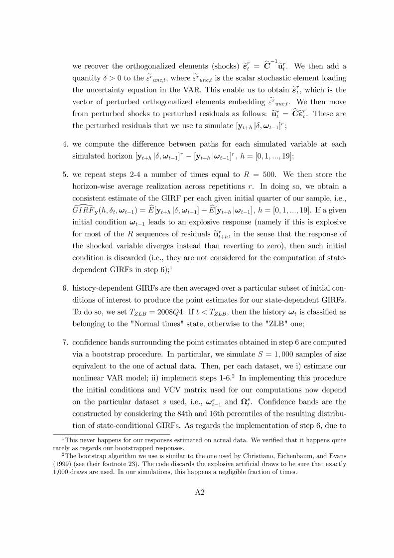
we recover the orthogonalized elements (shocks) e"rt = bC�1eurt . We then add aquantity � > 0 to the e"runc;t, where e"runc;t is the scalar stochastic element loadingthe uncertainty equation in the VAR. This enable us to obtain e"rt , which is thevector of perturbed orthogonalized elements embedding e"runc;t. We then movefrom perturbed shocks to perturbed residuals as follows: eurt = bCe"rt . These arethe perturbed residuals that we use to simulate [yt+h j�;!t�1]r ;

4. we compute the di¤erence between paths for each simulated variable at each

simulated horizon [yt+h j�;!t�1]r � [yt+h j!t�1]r , h = [0; 1; :::; 19];

5. we repeat steps 2-4 a number of times equal to R = 500. We then store the

horizon-wise average realization across repetitions r. In doing so, we obtain a

consistent estimate of the GIRF per each given initial quarter of our sample, i.e.,\GIRF y(h; �t;!t�1) = bE[yt+h j�;!t�1] � bE[yt+h j!t�1] , h = [0; 1; :::; 19]. If a giveninitial condition !t�1 leads to an explosive response (namely if this is explosive

for most of the R sequences of residuals eurt+h, in the sense that the response ofthe shocked variable diverges instead than reverting to zero), then such initial

condition is discarded (i.e., they are not considered for the computation of state-

dependent GIRFs in step 6);1

6. history-dependent GIRFs are then averaged over a particular subset of initial con-

ditions of interest to produce the point estimates for our state-dependent GIRFs.

To do so, we set TZLB = 2008Q4. If t < TZLB, then the history !t is classi�ed as

belonging to the "Normal times" state, otherwise to the "ZLB" one;

7. con�dence bands surrounding the point estimates obtained in step 6 are computed

via a bootstrap procedure. In particular, we simulate S = 1; 000 samples of size

equivalent to the one of actual data. Then, per each dataset, we i) estimate our

nonlinear VAR model; ii) implement steps 1-6.2 In implementing this procedure

the initial conditions and VCV matrix used for our computations now depend

on the particular dataset s used, i.e., !st�1 and st . Con�dence bands are the

constructed by considering the 84th and 16th percentiles of the resulting distribu-

tion of state-conditional GIRFs. As regards the implementation of step 6, due to

1This never happens for our responses estimated on actual data. We veri�ed that it happens quiterarely as regards our bootstrapped responses.

2The bootstrap algorithm we use is similar to the one used by Christiano, Eichenbaum, and Evans(1999) (see their footnote 23). The code discards the explosive arti�cial draws to be sure that exactly1,000 draws are used. In our simulations, this happens a negligible fraction of times.

A2

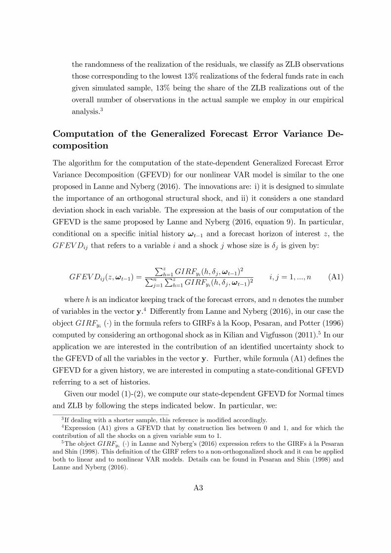
the randomness of the realization of the residuals, we classify as ZLB observations

those corresponding to the lowest 13% realizations of the federal funds rate in each

given simulated sample, 13% being the share of the ZLB realizations out of the

overall number of observations in the actual sample we employ in our empirical

analysis.3

Computation of the Generalized Forecast Error Variance De-composition

The algorithm for the computation of the state-dependent Generalized Forecast Error

Variance Decomposition (GFEVD) for our nonlinear VAR model is similar to the one

proposed in Lanne and Nyberg (2016). The innovations are: i) it is designed to simulate

the importance of an orthogonal structural shock, and ii) it considers a one standard

deviation shock in each variable. The expression at the basis of our computation of the

GFEVD is the same proposed by Lanne and Nyberg (2016, equation 9). In particular,

conditional on a speci�c initial history !t�1 and a forecast horizon of interest z, the

GFEVDij that refers to a variable i and a shock j whose size is �j is given by:

GFEVDij(z;!t�1) =

Pzh=1GIRFyi(h; �j;!t�1)

2Pnj=1

Pzh=1GIRFyi(h; �j;!t�1)

2i; j = 1; :::; n (A1)

where h is an indicator keeping track of the forecast errors, and n denotes the number

of variables in the vector y.4 Di¤erently from Lanne and Nyberg (2016), in our case the

object GIRFyi (�) in the formula refers to GIRFs à la Koop, Pesaran, and Potter (1996)computed by considering an orthogonal shock as in Kilian and Vigfusson (2011).5 In our

application we are interested in the contribution of an identi�ed uncertainty shock to

the GFEVD of all the variables in the vector y. Further, while formula (A1) de�nes the

GFEVD for a given history, we are interested in computing a state-conditional GFEVD

referring to a set of histories.

Given our model (1)-(2), we compute our state-dependent GFEVD for Normal times

and ZLB by following the steps indicated below. In particular, we:

3If dealing with a shorter sample, this reference is modi�ed accordingly.4Expression (A1) gives a GFEVD that by construction lies between 0 and 1, and for which the

contribution of all the shocks on a given variable sum to 1.5The object GIRFyi (�) in Lanne and Nyberg�s (2016) expression refers to the GIRFs à la Pesaran

and Shin (1998). This de�nition of the GIRF refers to a non-orthogonalized shock and it can be appliedboth to linear and to nonlinear VAR models. Details can be found in Pesaran and Shin (1998) andLanne and Nyberg (2016).

A3

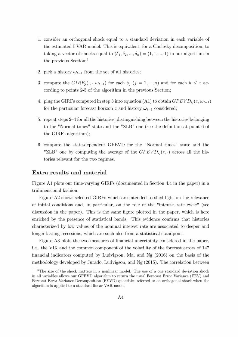
1. consider an orthogonal shock equal to a standard deviation in each variable of

the estimated I-VAR model. This is equivalent, for a Cholesky decomposition, to

taking a vector of shocks equal to (�1; �2; :::; �n) = (1; 1; :::; 1) in our algorithm in

the previous Section;6

2. pick a history !t�1 from the set of all histories;

3. compute the GIRFy(�; �;!t�1) for each �j (j = 1; :::; n) and for each h � z ac-

cording to points 2-5 of the algorithm in the previous Section;

4. plug the GIRFs computed in step 3 into equation (A1) to obtainGFEVDij(z;!t�1)

for the particular forecast horizon z and history !t�1 considered;

5. repeat steps 2�4 for all the histories, distinguishing between the histories belonging

to the "Normal times" state and the "ZLB" one (see the de�nition at point 6 of

the GIRFs algorithm);

6. compute the state-dependent GFEVD for the "Normal times" state and the

"ZLB" one by computing the average of the GFEVDij(z; �) across all the his-tories relevant for the two regimes.

Extra results and material

Figure A1 plots our time-varying GIRFs (documented in Section 4.4 in the paper) in a

tridimensional fashion.

Figure A2 shows selected GIRFs which are intended to shed light on the relevance

of initial conditions and, in particular, on the role of the "interest rate cycle" (see

discussion in the paper). This is the same �gure plotted in the paper, which is here

enriched by the presence of statistical bands. This evidence con�rms that histories

characterized by low values of the nominal interest rate are associated to deeper and

longer lasting recessions, which are such also from a statistical standpoint.

Figure A3 plots the two measures of �nancial uncertainty considered in the paper,

i.e., the VIX and the common component of the volatility of the forecast errors of 147

�nancial indicators computed by Ludvigson, Ma, and Ng (2016) on the basis of the

methodology developed by Jurado, Ludvigson, and Ng (2015). The correlation between

6The size of the shock matters in a nonlinear model. The use of a one standard deviation shockin all variables allows our GFEVD algorithm to return the usual Forecast Error Variance (FEV) andForecast Error Variance Decomposition (FEVD) quantities referred to an orthogonal shock when thealgorithm is applied to a standard linear VAR model.

A4

these two measures in our sample is 0.74. Notice that the VIX is available since 1990.

Following Bloom (2009), we consider the volatility of stock market returns as a proxy

for the VIX for the pre-1990 period.

Figure A4 refers to an exercise we conducted to be sure that our GIRFs related to

the ZLB period are not driven by non-uncertainty shocks. This exercise is conducted to

make sure that no shock which could have led to the ZLB keeps operating, possibly with

bigger strength, and drives the results which we instead attribute to the presence of the

ZLB. Figure A4 documents four scenarios for which we compute GIRFs by switching

o¤ one set of shocks at a time among the non-uncertainty ones. The sets refer to shocks

to prices, real GDP, investment, and consumption. The results documented in Figure

4 point to the irrelevance of these non-uncertainty shocks in the computation of the

GIRFs to an uncertainty shock.

Finally, Table A1 con�rms that the stylized fact studied in the paper - i.e., the

larger correlation between uncertainty and the growth rate of real GDP, investment,

and consumption - holds true when uncertainty indicators alternative to those employed

in the paper are considered.

ReferencesChristiano, L. J., M. Eichenbaum, and C. Evans (1999): �Monetary PolicyShocks: What Have We Learned and to What End?,�In: J.B. Taylor and M. Wood-ford (eds.): Handbook of Macroeconomics, Elsevier Science, 65�148.

Jurado, K., S. C. Ludvigson, and S. Ng (2015): �Measuring Uncertainty,�Amer-ican Economic Review, 105(3), 1177�1216.

Kilian, L., and R. Vigfusson (2011): �Are the Responses of the U.S. EconomyAsymmetric in Energy Price Increases and Decreases?,�Quantitative Economics, 2,419�453.

Koop, G., M. Pesaran, and S. Potter (1996): �Impulse response analysis innonlinear multivariate models,�Journal of Econometrics, 74(1), 119�147.

Lanne, M., and H. Nyberg (2016): �Generalised Forecast Error Variance Decompo-sition for Linear and Nonlinear Multivariate Models,�Oxford Bulletin of Economicsand Statistics, 78, 595�603.

Ludvigson, S. C., S. Ma, and S. Ng (2016): �Uncertainty and Business Cycles:Exogenous Impulse or Endogenous Response?,�New York University and ColumbiaUniversity, mimeo.

Pesaran, H. M., and Y. Shin (1998): �Generalized Impulse Response Analysis inLinear Multivariate Models,�Economics Letters, 58, 17�29.

A5

1968 1976 1984 1992 2000 2008 010

20­0.5

00.5

ZLBNormal times

GDP

1968 1976 1984 1992 2000 2008 010

20­202

ZLBNormal times

Investment

1968 1976 1984 1992 2000 2008 010

20­0.5

00.5

ZLBNormal times

Consumption

Figure A1: Time-varying GIRFs: Normal times vs. ZLB. Uncertainty proxied byVIX. Left column: Temporal evolution of the GIRFs. Colors ranging from blue (peakvalues per each given history) to red (trough values per each given history).

A6

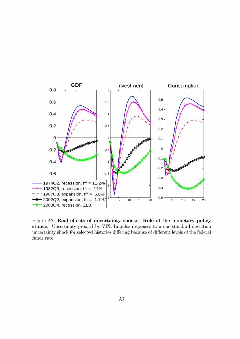
5 10 15 20­1

­0.8

­0.6

­0.4

­0.2

0

0.2

0.4

0.6

0.8GDP

1974Q2, recession, ffr = 11.2%1982Q3, recession, ffr =  11%1987Q3, expansion, ffr =  6.8%2002Q2, expansion, ffr =  1.7%2008Q4, recession, ZLB

5 10 15 20­2.5

­2

­1.5

­1

­0.5

0

0.5

1

1.5

2Investment

5 10 15 20­0.5

­0.4

­0.3

­0.2

­0.1

0

0.1

0.2

0.3

0.4

0.5

Consumption

Figure A2: Real e¤ects of uncertainty shocks: Role of the monetary policystance. Uncertainty proxied by VIX. Impulse responses to a one standard deviationuncertainty shock for selected histories di¤ering because of di¤erent levels of the federalfunds rate.

A7

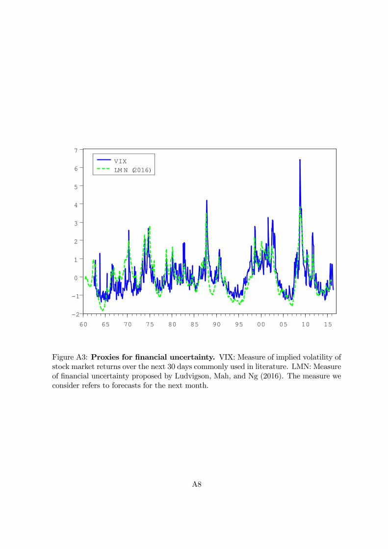
­2

­1

0

1

2

3

4

5

6

7

60 65 70 75 80 85 90 95 00 05 10 15

VIXLM N (2016)

Figure A3: Proxies for �nancial uncertainty. VIX: Measure of implied volatility ofstock market returns over the next 30 days commonly used in literature. LMN: Measureof �nancial uncertainty proposed by Ludvigson, Mah, and Ng (2016). The measure weconsider refers to forecasts for the next month.

A8

5 10 15 20­0.5

0

0.5

No P

r. sh

ocks

GDP

5 10 15 20­2

­1

0

1Investment

5 10 15 20­0.5

0

0.5ConsumptionNormal times: Baseline

ZLB: BaselineZLB: No future shocks

5 10 15 20­0.5

0

0.5

No G

DP s

hock

s

5 10 15 20­2

­1

0

1

5 10 15 20­0.5

0

0.5

5 10 15 20­0.5

0

0.5

No In

v. s

hock

s

5 10 15 20­2

­1

0

1

5 10 15 20­0.5

0

0.5

5 10 15 20­0.5

0

0.5

No C

ons.

 sho

cks

5 10 15 20­2

­1

0

1

5 10 15 20­0.5

0

0.5

Figure A4: GIRFs during the ZLB: Role of non-uncertainty shocks. Compari-son between GIRFs computed for the ZLB phase as in our baseline exercise and GIRFscomputed by muting four non-uncertainty shocks one at a time. Muted shocks: "NoPr. shocks" refers to the case in which shocks to prices are muted: "No GDP shocks"to the case in which shocks to real GDP are muted; "No Inv. shocks" refers to the casein which shocks to real investment are muted; "No Cons. shocks" refers to the case inwhch shocks to consumption are muted.

A9

Classi�c. Unc. indic. Period �Y=Y �I=I �C=CVIX Normal times -0.22 -0.19 -0.23

Financial ZLB -0.75 -0.63 -0.79uncertainty LMN Normal times -0.29 -0.26 -0.28

ZLB -0.60 -0.55 -0.67JLN Normal times -0.46 -0.36 -0.47

ZLB -0.74 -0.69 -0.75Macroecon. RS Normal times -0.13 -0.12 -0.11uncertainty ZLB -0.21 -0.36 -0.11

BBD Normal times -0.17 -0.14 -0.15ZLB -0.50 -0.45 -0.33

Table A1: Uncertainty-Real activity correlations: Normal times vs. ZLB.Real GDP, investment, and consumption considered in quarterly growth rates. Normaltimes: 1962Q3-2008Q3, ZLB: 2008Q4-2015Q4. Correlation coe¢ cients conditional onthe following periods: 1962Q3-2015Q4 - uncertainty proxied by the VIX, the �nancialuncertainty proxy estimated by Ludvigson, Ma, and Ng (2016) (LMN in the Table),the macroeconomic uncertainty proxy estimated by Jurado, Ludvigson, and Ng (2015)(JLN in the Table), and the economic policy uncertainty index built up by Baker,Bloom, and Davis (2016) (BBD in the Table); 1968Q4-2015Q1 - uncertainty proxied bythe Rossi and Sekhposyan (2015) index (RS in the Table); Di¤erences in samples dueto di¤erences in the availability of the uncertainty proxies. LMN�s and JLN�s proxiesrefer to an uncertainty horizon equal to one month. RS�s proxy refers to an uncertaintyhorizon equal to one year (revised version of the index).

A10