Creativeproblemsolvingpracticaltoolsfinal 131903461701-phpapp01-111019093051-phpapp01
Upload
vijendra-kumarCategory
view
6download
1description

MeetMinitab.book Page 1 Monday, April 6, 2009 11:25 AM

ii
© 2010 by Minitab, Inc. All rights reserved. Release 16.1.0
Minitab®, the Minitab logo®, Quality Companion by Minitab® and Quality Trainer by Minitab® are registered trademarks of Minitab, Inc. in the United States and other countries. Capability Sixpack™, Process Capability Sixpack™, ReportPad™, and StatGuide™ are all trademarks of Minitab, Inc.
Six Sigma® is a registered trademark and service mark of Motorola, Inc. All other marks referenced remain the property of their respective owners.
MeetMinitab.book Page 2 Monday, April 6, 2009 11:25 AM

iii
Table of Contents
1 Getting Started . . . . . . . . . . . . . . . . . . . . . . . . . . . . . . . . . . . . . . . . . . . . . .1-1Objectives . . . . . . . . . . . . . . . . . . . . . . . . . . . . . . . . . . . . . . . . . . . . . . . . . . . 1-1
Overview . . . . . . . . . . . . . . . . . . . . . . . . . . . . . . . . . . . . . . . . . . . . . . . . . . . . 1-1
Typographical Conventions in this Book . . . . . . . . . . . . . . . . . . . . . . . . . . . . . 1-2
The Story . . . . . . . . . . . . . . . . . . . . . . . . . . . . . . . . . . . . . . . . . . . . . . . . . . . . 1-3
Starting Minitab . . . . . . . . . . . . . . . . . . . . . . . . . . . . . . . . . . . . . . . . . . . . . . . 1-3
Opening a Worksheet. . . . . . . . . . . . . . . . . . . . . . . . . . . . . . . . . . . . . . . . . . . 1-4
What’s Next . . . . . . . . . . . . . . . . . . . . . . . . . . . . . . . . . . . . . . . . . . . . . . . . . . 1-6
2 Graphing Data . . . . . . . . . . . . . . . . . . . . . . . . . . . . . . . . . . . . . . . . . . . . . .2-1Objectives . . . . . . . . . . . . . . . . . . . . . . . . . . . . . . . . . . . . . . . . . . . . . . . . . . . 2-1
Overview . . . . . . . . . . . . . . . . . . . . . . . . . . . . . . . . . . . . . . . . . . . . . . . . . . . . 2-1
Exploring the Data . . . . . . . . . . . . . . . . . . . . . . . . . . . . . . . . . . . . . . . . . . . . . 2-2
Examining Relationships Between Two Variables. . . . . . . . . . . . . . . . . . . . . . . 2-8
Using Graph Layout and Printing . . . . . . . . . . . . . . . . . . . . . . . . . . . . . . . . . 2-11
Saving Projects . . . . . . . . . . . . . . . . . . . . . . . . . . . . . . . . . . . . . . . . . . . . . . . 2-13
What’s Next . . . . . . . . . . . . . . . . . . . . . . . . . . . . . . . . . . . . . . . . . . . . . . . . . 2-14
3 Analyzing Data . . . . . . . . . . . . . . . . . . . . . . . . . . . . . . . . . . . . . . . . . . . . . .3-1Objectives . . . . . . . . . . . . . . . . . . . . . . . . . . . . . . . . . . . . . . . . . . . . . . . . . . . 3-1
Overview . . . . . . . . . . . . . . . . . . . . . . . . . . . . . . . . . . . . . . . . . . . . . . . . . . . . 3-1
Displaying Descriptive Statistics . . . . . . . . . . . . . . . . . . . . . . . . . . . . . . . . . . . 3-2
Performing an ANOVA . . . . . . . . . . . . . . . . . . . . . . . . . . . . . . . . . . . . . . . . . . 3-4
Using Minitab’s Project Manager . . . . . . . . . . . . . . . . . . . . . . . . . . . . . . . . . . 3-8
What’s Next . . . . . . . . . . . . . . . . . . . . . . . . . . . . . . . . . . . . . . . . . . . . . . . . . 3-11
4 Assessing Quality . . . . . . . . . . . . . . . . . . . . . . . . . . . . . . . . . . . . . . . . . . . . .4-1Objectives . . . . . . . . . . . . . . . . . . . . . . . . . . . . . . . . . . . . . . . . . . . . . . . . . . . 4-1
Overview . . . . . . . . . . . . . . . . . . . . . . . . . . . . . . . . . . . . . . . . . . . . . . . . . . . . 4-1
Evaluating Process Stability . . . . . . . . . . . . . . . . . . . . . . . . . . . . . . . . . . . . . . . 4-2
Evaluating Process Capability . . . . . . . . . . . . . . . . . . . . . . . . . . . . . . . . . . . . . 4-8
What’s Next . . . . . . . . . . . . . . . . . . . . . . . . . . . . . . . . . . . . . . . . . . . . . . . . . 4-10
MeetMinitab.book Page iii Monday, April 6, 2009 11:25 AM

iv
5 Designing an Experiment . . . . . . . . . . . . . . . . . . . . . . . . . . . . . . . . . . . . . 5-1Objectives . . . . . . . . . . . . . . . . . . . . . . . . . . . . . . . . . . . . . . . . . . . . . . . . . . . 5-1
Overview . . . . . . . . . . . . . . . . . . . . . . . . . . . . . . . . . . . . . . . . . . . . . . . . . . . 5-1
Creating an Experimental Design . . . . . . . . . . . . . . . . . . . . . . . . . . . . . . . . . 5-2
Viewing the Design. . . . . . . . . . . . . . . . . . . . . . . . . . . . . . . . . . . . . . . . . . . . 5-5
Entering Data . . . . . . . . . . . . . . . . . . . . . . . . . . . . . . . . . . . . . . . . . . . . . . . . 5-5
Analyzing the Design . . . . . . . . . . . . . . . . . . . . . . . . . . . . . . . . . . . . . . . . . . 5-6
Drawing Conclusions . . . . . . . . . . . . . . . . . . . . . . . . . . . . . . . . . . . . . . . . . . 5-9
What’s Next . . . . . . . . . . . . . . . . . . . . . . . . . . . . . . . . . . . . . . . . . . . . . . . . 5-12
6 Using Session Commands . . . . . . . . . . . . . . . . . . . . . . . . . . . . . . . . . . . . . 6-1Objectives . . . . . . . . . . . . . . . . . . . . . . . . . . . . . . . . . . . . . . . . . . . . . . . . . . . 6-1
Overview . . . . . . . . . . . . . . . . . . . . . . . . . . . . . . . . . . . . . . . . . . . . . . . . . . . 6-1
Enabling and Typing Commands . . . . . . . . . . . . . . . . . . . . . . . . . . . . . . . . . 6-2
Rerunning a Series of Commands . . . . . . . . . . . . . . . . . . . . . . . . . . . . . . . . . 6-5
Repeating Analyses with Execs . . . . . . . . . . . . . . . . . . . . . . . . . . . . . . . . . . . 6-6
What’s Next . . . . . . . . . . . . . . . . . . . . . . . . . . . . . . . . . . . . . . . . . . . . . . . . . 6-8
7 Generating a Report . . . . . . . . . . . . . . . . . . . . . . . . . . . . . . . . . . . . . . . . . . 7-1Objectives . . . . . . . . . . . . . . . . . . . . . . . . . . . . . . . . . . . . . . . . . . . . . . . . . . . 7-1
Overview . . . . . . . . . . . . . . . . . . . . . . . . . . . . . . . . . . . . . . . . . . . . . . . . . . . 7-1
Using the ReportPad . . . . . . . . . . . . . . . . . . . . . . . . . . . . . . . . . . . . . . . . . . . 7-2
Saving a Report. . . . . . . . . . . . . . . . . . . . . . . . . . . . . . . . . . . . . . . . . . . . . . . 7-6
Copying a Report to a Word Processor . . . . . . . . . . . . . . . . . . . . . . . . . . . . . 7-6
Using Embedded Graph Editing Tools . . . . . . . . . . . . . . . . . . . . . . . . . . . . . . 7-7
Sending Output to Microsoft PowerPoint . . . . . . . . . . . . . . . . . . . . . . . . . . . 7-9
What’s Next . . . . . . . . . . . . . . . . . . . . . . . . . . . . . . . . . . . . . . . . . . . . . . . . 7-11
8 Preparing a Worksheet . . . . . . . . . . . . . . . . . . . . . . . . . . . . . . . . . . . . . . . . 8-1Objectives . . . . . . . . . . . . . . . . . . . . . . . . . . . . . . . . . . . . . . . . . . . . . . . . . . . 8-1
Overview . . . . . . . . . . . . . . . . . . . . . . . . . . . . . . . . . . . . . . . . . . . . . . . . . . . 8-1
Getting Data from Different Sources . . . . . . . . . . . . . . . . . . . . . . . . . . . . . . . 8-2
Preparing the Worksheet for Analysis. . . . . . . . . . . . . . . . . . . . . . . . . . . . . . . 8-4
What’s Next . . . . . . . . . . . . . . . . . . . . . . . . . . . . . . . . . . . . . . . . . . . . . . . . 8-11
MeetMinitab.book Page iv Monday, April 6, 2009 11:25 AM

v
9 Customizing Minitab . . . . . . . . . . . . . . . . . . . . . . . . . . . . . . . . . . . . . . . . .9-1Objectives . . . . . . . . . . . . . . . . . . . . . . . . . . . . . . . . . . . . . . . . . . . . . . . . . . . 9-1
Overview . . . . . . . . . . . . . . . . . . . . . . . . . . . . . . . . . . . . . . . . . . . . . . . . . . . . 9-1
Setting Options . . . . . . . . . . . . . . . . . . . . . . . . . . . . . . . . . . . . . . . . . . . . . . . 9-2
Creating a Custom Toolbar . . . . . . . . . . . . . . . . . . . . . . . . . . . . . . . . . . . . . . 9-3
Assigning Shortcut Keys . . . . . . . . . . . . . . . . . . . . . . . . . . . . . . . . . . . . . . . . . 9-5
Restoring Minitab’s Default Settings . . . . . . . . . . . . . . . . . . . . . . . . . . . . . . . . 9-6
What’s Next . . . . . . . . . . . . . . . . . . . . . . . . . . . . . . . . . . . . . . . . . . . . . . . . . . 9-7
10 Getting Help . . . . . . . . . . . . . . . . . . . . . . . . . . . . . . . . . . . . . . . . . . . . . .10-1Objectives . . . . . . . . . . . . . . . . . . . . . . . . . . . . . . . . . . . . . . . . . . . . . . . . . . 10-1
Overview . . . . . . . . . . . . . . . . . . . . . . . . . . . . . . . . . . . . . . . . . . . . . . . . . . . 10-1
Getting Answers and Information . . . . . . . . . . . . . . . . . . . . . . . . . . . . . . . . . 10-2
Minitab Help Overview. . . . . . . . . . . . . . . . . . . . . . . . . . . . . . . . . . . . . . . . . 10-4
Help . . . . . . . . . . . . . . . . . . . . . . . . . . . . . . . . . . . . . . . . . . . . . . . . . . . . . . . 10-6
StatGuide . . . . . . . . . . . . . . . . . . . . . . . . . . . . . . . . . . . . . . . . . . . . . . . . . . . 10-8
Session Command Help . . . . . . . . . . . . . . . . . . . . . . . . . . . . . . . . . . . . . . . 10-10
What’s Next . . . . . . . . . . . . . . . . . . . . . . . . . . . . . . . . . . . . . . . . . . . . . . . . 10-11
11 Reference . . . . . . . . . . . . . . . . . . . . . . . . . . . . . . . . . . . . . . . . . . . . . . . .11-1Objectives . . . . . . . . . . . . . . . . . . . . . . . . . . . . . . . . . . . . . . . . . . . . . . . . . . 11-1
Overview . . . . . . . . . . . . . . . . . . . . . . . . . . . . . . . . . . . . . . . . . . . . . . . . . . . 11-1
The Minitab Environment . . . . . . . . . . . . . . . . . . . . . . . . . . . . . . . . . . . . . . . 11-2
Minitab Data . . . . . . . . . . . . . . . . . . . . . . . . . . . . . . . . . . . . . . . . . . . . . . . . 11-5
Index . . . . . . . . . . . . . . . . . . . . . . . . . . . . . . . . . . . . . . . . . . . . . . . . . . . . . . . . I-1
MeetMinitab.book Page v Monday, April 6, 2009 11:25 AM

vi
MeetMinitab.book Page vi Monday, April 6, 2009 11:25 AM

Meet Minitab 1-1
1Getting Started
ObjectivesIn this chapter, you:
■ Learn how to use Meet Minitab, page 1-1
■ Start Minitab, page 1-3
■ Open and examine a worksheet, page 1-4
OverviewMeet Minitab introduces you to the most commonly used features in Minitab. Throughout the book, you use functions, create graphs, and generate statistics. The contents of Meet Minitab relate to the actions you need to perform in your own Minitab sessions. You use a sampling of Minitab’s features to see the range of features and statistics that Minitab provides.
Most statistical analyses require a series of steps, often directed by background knowledge or by the subject area you are investigating. Chapters 2 through 5 illustrate the analysis steps in a typical Minitab session:
■ Exploring data with graphs
■ Conducting statistical analyses and procedures
■ Assessing quality
■ Designing an experiment
Chapters 6 through 9 provide information on:
■ Using shortcuts to automate future analyses
■ Generating a report
■ Preparing worksheets
■ Customizing Minitab to fit your needs
MeetMinitab.book Page 1 Monday, April 6, 2009 11:25 AM

Chapter 1 Typographical Conventions in this Book
1-2 Meet Minitab
Chapter 10, Getting Help, includes information on getting answers and using Minitab Help features. Chapter 11, Reference, provides an overview of the Minitab environment and a discussion about the types and forms of data that Minitab uses.
You can work through Meet Minitab in two ways:
■ From beginning to end, following the story of a fictional online bookstore through a common workflow
■ By selecting a specific chapter to familiarize yourself with a particular area of Minitab
Meet Minitab introduces dialog boxes and windows when you need them to perform a step in the analysis. As you work, look for these icons for additional information:
Provides notes and tips
Suggests related topics in Minitab Help and StatGuide
Typographical Conventions in this Book[Enter] Denotes a key, such as the [Enter] key.
[Alt]+[D] Denotes holding down the first key and pressing the second key. For example, while holding down the [Alt] key, press the [D] key.
File ➤ Exit Denotes a menu command, in this case choose Exit from the File menu. Here is another example: Stat ➤ Tables ➤ Tally Individual Variables means open the Stat menu, then open the Tables submenu, and finally choose Tally Individual Variables.
Click OK. Bold text clarifies dialog box items and buttons and Minitab commands.
Enter Pulse1. Italic text specifies text you need to enter.
MeetMinitab.book Page 2 Monday, April 6, 2009 11:25 AM
The Story Getting Started
Meet Minitab 1-3
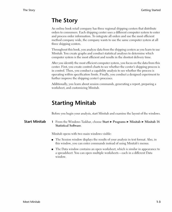
The StoryAn online book retail company has three regional shipping centers that distribute orders to consumers. Each shipping center uses a different computer system to enter and process order information. To integrate all orders and use the most efficient method company wide, the company wants to use the same computer system at all three shipping centers.
Throughout this book, you analyze data from the shipping centers as you learn to use Minitab. You create graphs and conduct statistical analyses to determine which computer system is the most efficient and results in the shortest delivery time.
After you identify the most efficient computer system, you focus on the data from this center. First, you create control charts to see whether the center’s shipping process is in control. Then, you conduct a capability analysis to see whether the process is operating within specification limits. Finally, you conduct a designed experiment to further improve the shipping center’s processes.
Additionally, you learn about session commands, generating a report, preparing a worksheet, and customizing Minitab.
Starting Minitab
Before you begin your analysis, start Minitab and examine the layout of the windows.
Start Minitab 1 From the Windows Taskbar, choose Start ➤ Programs ➤ Minitab ➤ Minitab 16 Statistical Software.
Minitab opens with two main windows visible:
■ The Session window displays the results of your analysis in text format. Also, in this window, you can enter commands instead of using Minitab’s menus.
■ The Data window contains an open worksheet, which is similar in appearance to a spreadsheet. You can open multiple worksheets—each in a different Data window.
MeetMinitab.book Page 3 Monday, April 6, 2009 11:25 AM
Chapter 1 Opening a Worksheet
1-4 Meet Minitab
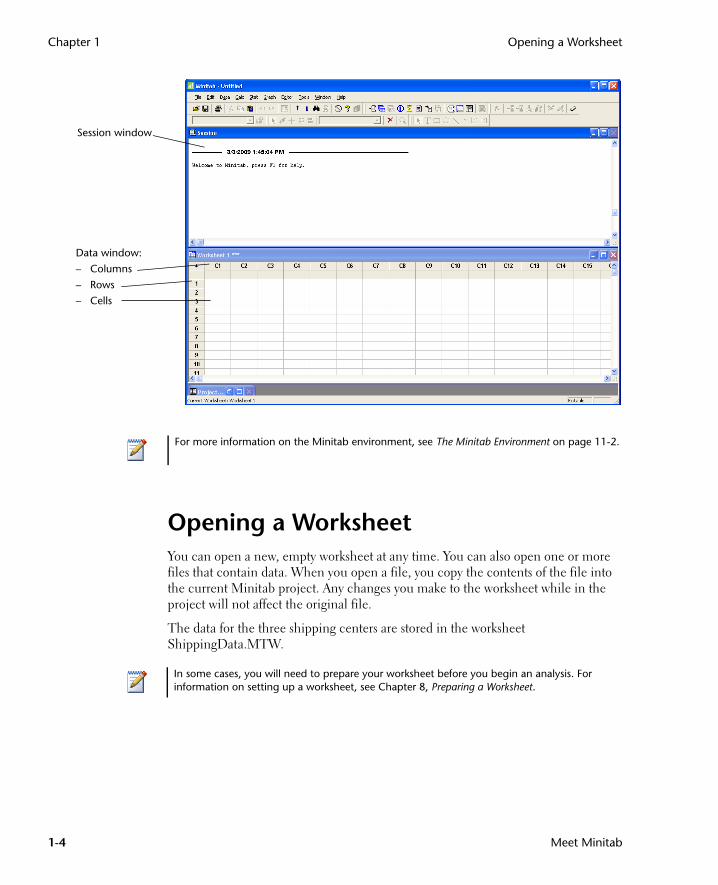
Opening a WorksheetYou can open a new, empty worksheet at any time. You can also open one or more files that contain data. When you open a file, you copy the contents of the file into the current Minitab project. Any changes you make to the worksheet while in the project will not affect the original file.
The data for the three shipping centers are stored in the worksheet ShippingData.MTW.
Data window:
– Columns
– Rows
– Cells
Session window
For more information on the Minitab environment, see The Minitab Environment on page 11-2.
In some cases, you will need to prepare your worksheet before you begin an analysis. For information on setting up a worksheet, see Chapter 8, Preparing a Worksheet.
MeetMinitab.book Page 4 Monday, April 6, 2009 11:25 AM

Opening a Worksheet Getting Started
Meet Minitab 1-5
Open aworksheet
1 Choose File ➤ Open Worksheet.
2 Click Look in Minitab Sample Data folder, near the bottom of the dialog box.
3 In the Sample Data folder, double-click Meet Minitab.
You can change the default folder for opening and saving Minitab files by choosing Tools ➤ Options ➤ General.
4 Choose ShippingData.MTW, then click Open. If you get a message box, check Do not display this message again, then click OK. To restore this message for every time you open a worksheet, return to Minitab’s default settings. See Restoring Minitab’s Default Settings on page 9-6.
Examineworksheet
The data are arranged in columns, which are also called variables. The column number and name are at the top of each column. Each row in the worksheet represents a case, which is information on a single book order.
Minitab accepts three types of data: numeric, text, and date/time. This worksheet contains each type.
The data include:
■ Shipping center name
■ Order date
■ Delivery date
Column with date/time data
Column name
Column with numeric data
Column with text data
Row number
MeetMinitab.book Page 5 Monday, April 6, 2009 11:25 AM

Chapter 1 What’s Next
1-6 Meet Minitab
■ Number of delivery days
■ Delivery status (“On time” indicates that the book shipment was received on time; “Back order” indicates that the book is not currently in stock; “Late” indicates that the book shipment was received six or more days after ordered)
■ Distance from shipping center to delivery location
What’s NextNow that you have a worksheet open, you are ready to start using Minitab. In the next chapter, you use graphs to check the data for normality and examine the relationships between variables.
For more information about data types, see Minitab Data on page 11-5.
MeetMinitab.book Page 6 Monday, April 6, 2009 11:25 AM
Meet Minitab 2-1
2Graphing Data
ObjectivesIn this chapter, you:
■ Create and interpret an individual value plot, page 2-2
■ Create a histogram with groups, page 2-4
■ Edit a histogram, page 2-5
■ Arrange multiple histograms on the same page, page 2-6
■ Access Help, page 2-8
■ Create and interpret scatterplots, page 2-9
■ Edit a scatterplot, page 2-10
■ Arrange multiple graphs on the same page, page 2-12
■ Print graphs, page 2-13
■ Save a project, page 2-13
OverviewBefore conducting a statistical analysis, you can use graphs to explore data and assess relationships among the variables. Also, graphs are useful to summarize findings and to ease interpretation of statistical results.
You can access Minitab’s graphs from the Graph and Stat menus. Built-in graphs, which help you to interpret results and assess the validity of statistical assumptions, are also available with many statistical commands.
Graph features in Minitab include:
■ A pictorial gallery from which to choose a graph type
■ Flexibility in customizing graphs, from subsetting of data to specifying titles and footnotes
MeetMinitab.book Page 1 Monday, April 6, 2009 11:25 AM

Chapter 2 Exploring the Data
2-2 Meet Minitab
■ Ability to change most graph elements, such as fonts, symbols, lines, placement of tick marks, and data display, after the graph is created
■ Ability to automatically update graphs
This chapter explores the shipping center data you opened in the previous chapter, using graphs to compare means, explore variability, check normality, and examine the relationship between variables.
Exploring the DataBefore conducting a statistical analysis, you should first create graphs that display important characteristics of the data.
For the shipping center data, you want to know the mean delivery time for each shipping center and how variable the data are within each shipping center. You also want to determine if the shipping center data follow a normal distribution so you that you can use standard statistical methods for testing the equality of means.
Create anindividualvalue plot
You suspect that delivery time is different for the three shipping centers. Create an individual value plot to compare the shipping center data.
1 If not continuing from the previous chapter, choose File ➤ Open Worksheet. If continuing from the previous chapter, go to step 4.
2 Click Look in Minitab Sample Data folder, near the bottom of the dialog box.
3 In the Sample Data folder, double-click Meet Minitab, then choose ShippingData.MTW. Click Open.
4 Choose Graph ➤ Individual Value Plot.
For most graphs, Minitab displays a pictorial gallery. Your gallery choice determines the available graph creation options.
5 Under One Y, choose With Groups, then click OK.
For more information on Minitab graphs, go to Graphs in the Minitab Help index and then double-click the Overview entry for details on Minitab graphs. To access the Help index, choose Help ➤ Help, then click the Index tab.
MeetMinitab.book Page 2 Monday, April 6, 2009 11:25 AM

Exploring the Data Graphing Data
Meet Minitab 2-3
6 In Graph variables, enter Days.
7 In Categorical variables for grouping (1-4, outermost first), enter Center.
To create a graph, you only need to complete the main dialog box. However, you can click any button to open dialog boxes to customize your graph.
The list box on the left shows the variables from the worksheet that are available for the analysis. The boxes on the right display the variables that you select for the analysis.
8 Click Data View. Check Mean connect line.
9 Click OK in each dialog box.
Graphwindowoutput
To select variables in most Minitab dialog boxes, you can: double-click the variables in the variables list box; highlight the variables in the list box, then choose Select; or type the variables’ names or column numbers.
MeetMinitab.book Page 3 Monday, April 6, 2009 11:25 AM

Chapter 2 Exploring the Data
2-4 Meet Minitab
Interpretresults
The individual value plots show that each center has a different mean delivery time. The Western center has a lower shipping time than the Central and Eastern centers. The variation within each shipping center seems about the same.
Create agrouped
histogram
Another way to compare the three shipping centers is to create a grouped histogram, which displays the histograms for each center on the same graph. The grouped histogram will show how much the data from each shipping center overlap.
1 Choose Graph ➤ Histogram.
2 Choose With Fit And Groups, then click OK.
3 In Graph variables, enter Days.
4 In Categorical variables for grouping (0-3), enter Center.
5 Click OK.
Graphwindowoutput
MeetMinitab.book Page 4 Monday, April 6, 2009 11:25 AM

Exploring the Data Graphing Data
Meet Minitab 2-5
Interpretresults
As you saw in the individual value plot, the means for each center are different. The mean delivery times are:
Central—3.984 days
Eastern—4.452 days
Western—2.981 days
The grouped histogram shows that the Central and Eastern centers are similar in mean delivery time and spread of delivery time. In contrast, the Western center mean delivery time is shorter and less spread out. Chapter 3, Analyzing Data, shows how to detect stastistically significant differences among means using analysis of variance.
Edithistogram
Editing graphs in Minitab is easy. You can edit virtually any graph element. For the histogram you just created, you want to:
■ Make the header text in the legend (the table with the center information) bold
■ Modify the title
Change the legend table header font
1 Double-click the legend.
2 Click the Header Font tab.
3 Under Style, check Bold.
4 Click OK.
Change the title
1 Double-click the title (Histogram of Days).
2 In Text, type Histogram of Delivery Time.
3 Click OK.
If your data change, Minitab can automatically update graphs. For more information, go to Updating graphs in the Minitab Help index.
MeetMinitab.book Page 5 Monday, April 6, 2009 11:25 AM

Chapter 2 Exploring the Data
2-6 Meet Minitab
Graphwindowoutput
Interpretresults
The histogram now features a bold font for the legend heading and a more descriptive title.
Create apaneled
histogram
To determine if the shipping center data follow a normal distribution, create a paneled histogram of the time lapse between order and delivery date.
1 Choose Graph ➤ Histogram.
2 Choose With Fit, then click OK.
In addition to editing individual graphs, you can change the default settings for future graphs.
■ To affect general graph settings, such as font attributes, graph size, and line types, choose Tools ➤ Options ➤ Graphics.
■ To affect graph-specific settings, such as the scale type on histograms or the method for calculating the plotted points on probability plots, choose Tools ➤ Options ➤ Individual Graphs.
The next time you open an affected dialog box, your preferences are reflected.
MeetMinitab.book Page 6 Monday, April 6, 2009 11:25 AM

Exploring the Data Graphing Data
Meet Minitab 2-7
3 In Graph variables, enter Days.
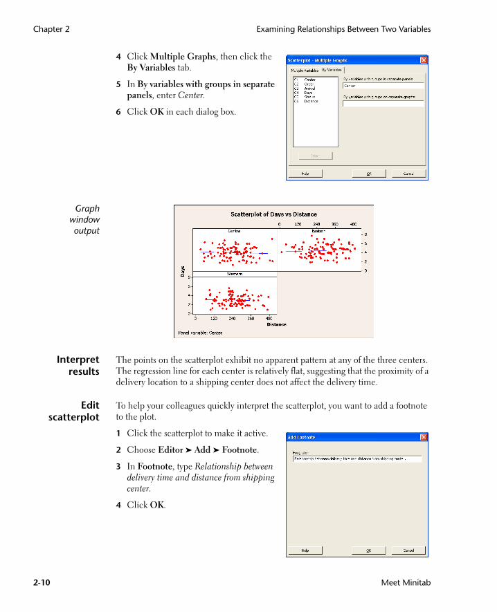
4 Click Multiple Graphs, then click the By Variables tab.
5 In By variables with groups in separate panels, enter Center.
6 Click OK in each dialog box.
Graphwindowoutput
Interpretresults
The delivery times for each center are approximately normally distributed as shown by the distribution curves exhibiting the same pattern.
If you have fewer than 50 observations, you may want to use a normal probability plot (Graph ➤ Probability Plot) to assess normality.
MeetMinitab.book Page 7 Monday, April 6, 2009 11:25 AM

Chapter 2 Examining Relationships Between Two Variables
2-8 Meet Minitab
Examining Relationships Between Two VariablesGraphs can help identify whether associations are present among variables and the strength of any associations. Knowing the relationship among variables can help to guide further analyses and determine which variables are important to analyze.
Because each shipping center serves a small regional delivery area, you suspect that distance to delivery site does not greatly affect delivery time. To verify this suspicion and eliminate distance as a potentially important factor, examine the relationship between delivery time and delivery distance.
Access Help To find out which graph shows the relationship between two variables, use Minitab Help.
1 Choose Help ➤ Help.
2 Click the Index tab.
3 In Type in the keyword to find, type Graphs and then double-click the Overview entry to access the Help topic.
4 In the Help topic, under the heading Types of graphs, click Examine relationships between pairs of variables.
MeetMinitab.book Page 8 Monday, April 6, 2009 11:25 AM

Examining Relationships Between Two Variables Graphing Data
Meet Minitab 2-9
This Help topic suggests that a scatterplot is the best choice to see the relationship between delivery time and delivery distance.
Create ascatterplot
1 Choose Graph ➤ Scatterplot.
2 Choose With Regression, then click OK.
3 Under Y variables, enter Days. Under X variables, enter Distance.
For help on any Minitab dialog box, click Help in the lower left corner of the dialog box or press [F1]. For more information on Minitab Help, see Chapter 10, Getting Help.
MeetMinitab.book Page 9 Monday, April 6, 2009 11:25 AM
Chapter 2 Examining Relationships Between Two Variables
2-10 Meet Minitab
4 Click Multiple Graphs, then click the By Variables tab.
5 In By variables with groups in separate panels, enter Center.
6 Click OK in each dialog box.
Graphwindowoutput
Interpretresults
The points on the scatterplot exhibit no apparent pattern at any of the three centers. The regression line for each center is relatively flat, suggesting that the proximity of a delivery location to a shipping center does not affect the delivery time.
Editscatterplot
To help your colleagues quickly interpret the scatterplot, you want to add a footnote to the plot.
1 Click the scatterplot to make it active.
2 Choose Editor ➤ Add ➤ Footnote.
3 In Footnote, type Relationship between delivery time and distance from shipping center.
4 Click OK.
MeetMinitab.book Page 10 Monday, April 6, 2009 11:25 AM

Using Graph Layout and Printing Graphing Data
Meet Minitab 2-11
Graphwindowoutput
Interpretresults
The scatterplot now features a footnote that provides a brief interpretation of the results.
Using Graph Layout and PrintingUse Minitab’s graph layout tool to place multiple graphs on the same page. You can add annotations to the layout and edit the individual graphs within the layout.
To show your supervisor the preliminary results of the graphical analysis of the shipping data, display all four graphs on one page.
When you issue a Minitab command that you previously used in the same session, Minitab remembers the dialog box settings. To set a dialog box back to its defaults, press [F3].
MeetMinitab.book Page 11 Monday, April 6, 2009 11:25 AM
Chapter 2 Using Graph Layout and Printing
2-12 Meet Minitab
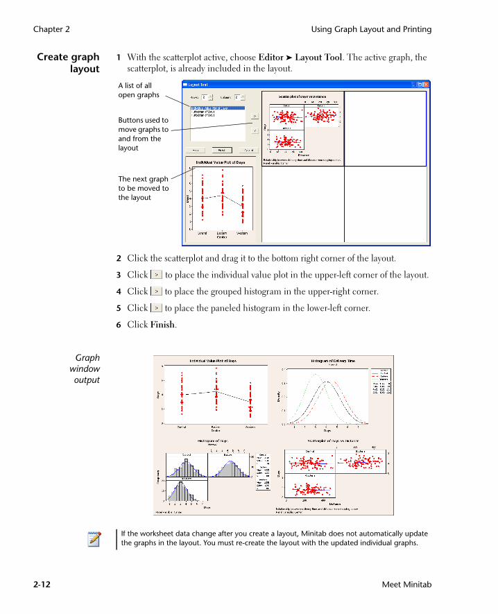
Create graphlayout
1 With the scatterplot active, choose Editor ➤ Layout Tool. The active graph, the scatterplot, is already included in the layout.
2 Click the scatterplot and drag it to the bottom right corner of the layout.
3 Click to place the individual value plot in the upper-left corner of the layout.
4 Click to place the grouped histogram in the upper-right corner.
5 Click to place the paneled histogram in the lower-left corner.
6 Click Finish.
Graphwindowoutput
A list of all open graphs
Buttons used to move graphs to and from the layout
The next graph to be moved to the layout
If the worksheet data change after you create a layout, Minitab does not automatically update the graphs in the layout. You must re-create the layout with the updated individual graphs.
MeetMinitab.book Page 12 Monday, April 6, 2009 11:25 AM

Saving Projects Graphing Data
Meet Minitab 2-13
Annotate thelayout
You want to add a descriptive title to the layout.
1 Choose Editor ➤ Add ➤ Title.
2 In Title, type Graphical Analysis of Shipping Center Data. Click OK.
Graphwindowoutput
Print graphlayout
You can print an individual graph or a layout just as you would any other Minitab window.
1 Click the Graph window to make it active, then choose File ➤ Print Graph.
2 Click OK.
Saving ProjectsMinitab data are saved in worksheets. You can also save Minitab projects which can contain multiple worksheets. A Minitab project contains all your work, including the data, Session window output, graphs, history of your session, ReportPad contents, and dialog box settings. When you open a project, you can resume working where you left off.
It is a good practice to save your work to a location outside the Program Files folder. While working through this book, files are saved to a Meet Minitab folder in the My Documents folder. You can save files to a location of your choice (outside the Program Files folder).
MeetMinitab.book Page 13 Monday, April 6, 2009 11:25 AM

Chapter 2 What’s Next
2-14 Meet Minitab
Save aMinitabproject
Save all of your work in a Minitab project.
1 Choose File ➤ Save Project As.
2 Navigate to the folder in which you want to save your files.
3 In File name, type My_Graphs.MPJ. Minitab automatically adds the extension .MPJ to the file name when you save the project.
4 Click Save.
What’s NextThe graphical output indicates that the three shipping centers have different delivery times for book orders. In the next chapter, you display descriptive statistics and perform an analysis of variance (ANOVA) to test whether the differences among the shipping centers are statistically significant.
If you close a project before saving it, Minitab prompts you to save the project.
MeetMinitab.book Page 14 Monday, April 6, 2009 11:25 AM
Meet Minitab 3-1
3Analyzing Data
ObjectivesIn this chapter, you:
■ Display and interpret descriptive statistics, page 3-2
■ Perform and interpret a one-way ANOVA, page 3-4
■ Display and interpret built-in graphs, page 3-4
■ Access the StatGuide, page 3-8
■ Use the Project Manager, page 3-8
OverviewThe field of statistics provides principles and methodologies for collecting, summarizing, analyzing, and interpreting data, and for drawing conclusions from analysis results. Statistics can be used to describe data and to make inferences, both of which can guide decisions and improve processes and products.
Minitab provides:
■ Many statistical methods organized by category, such as regression, ANOVA, quality tools, and time series
■ Built-in graphs to help you understand the data and validate results
■ The ability to display and store statistics and diagnostic measures
This chapter introduces Minitab’s statistical commands, built-in graphs, StatGuide, and Project Manager. You want to assess the number of late and back orders, and test whether the difference in delivery time among the three shipping centers is statistically significant.
For more information on Minitab’S statistical features, go to Stat menu in the Minitab Help index.
MeetMinitab.book Page 1 Monday, April 6, 2009 11:25 AM

Chapter 3 Displaying Descriptive Statistics
3-2 Meet Minitab
Displaying Descriptive StatisticsDescriptive statistics summarize and describe the prominent features of data.
Use Display Descriptive Statistics to find out how many book orders were delivered on time, how many were late, and the number that were initially back ordered for each shipping center.
Displaydescriptive
statistics
1 If continuing from the previous chapter, choose File ➤ New, then choose Minitab Project. Click OK. Otherwise, just start Minitab.
2 Choose File ➤ Open Worksheet.
3 Click Look in Minitab Sample Data folder, near the bottom of the dialog box.
4 In the Sample Data folder, double-click Meet Minitab, then choose ShippingData.MTW. Click Open. This worksheet is the same one you used in Chapter 2, Graphing Data.
5 Choose Stat ➤ Basic Statistics ➤ Display Descriptive Statistics.
6 In Variables, enter Days.
7 In By variables (optional), enter Center Status.
For most Minitab commands, you only need to complete the main dialog box to execute the command. But, you can often use subdialog boxes to modify the analysis or display additional output, like graphs.
8 Click Statistics.
9 Uncheck First quartile, Median, Third quartile, N nonmissing, and N missing.
10 Check N total.
11 Click OK in each dialog box.
Changes made in the Statistics subdialog box affect the current session only. To change the default settings for future sessions, use Tools ➤ Options ➤ Individual Commands ➤ Display Descriptive Statistics. When you open the Statistics subdialog box again, it reflects your preferences.
MeetMinitab.book Page 2 Monday, April 6, 2009 11:25 AM

Displaying Descriptive Statistics Analyzing Data
Meet Minitab 3-3
Sessionwindowoutput
Descriptive Statistics: Days Results for Center = Central
TotalVariable Status Count Mean SE Mean StDev Minimum MaximumDays Back order 6 * * * * * Late 6 6.431 0.157 0.385 6.078 7.070 On time 93 3.826 0.119 1.149 1.267 5.983
Results for Center = Eastern
TotalVariable Status Count Mean SE Mean StDev Minimum MaximumDays Back order 8 * * * * * Late 9 6.678 0.180 0.541 6.254 7.748 On time 92 4.234 0.112 1.077 1.860 5.953
Results for Center = Western
TotalVariable Status Count Mean SE Mean StDev Minimum MaximumDays Back order 3 * * * * * On time 102 2.981 0.108 1.090 0.871 5.681
Interpretresults
The Session window presents each center’s results separately. Within each center, you can find the number of back, late, and on-time orders in the Total Count column.
■ The Eastern shipping center has the most back orders (8) and late orders (9).
■ The Central shipping center has the next greatest number of back orders (6) and late orders (6).
■ The Western shipping center has the smallest number of back orders (3) and no late orders.
You can also review the Session window output for the mean, standard error of the mean, standard deviation, minimum, and maximum of order status for each center. These statistics are not given for back orders because no delivery information exists for these orders.
The Session window displays text output, which you can edit, add to the ReportPad, and print. The ReportPad is discussed in Chapter 7, Generating a Report.
MeetMinitab.book Page 3 Monday, April 6, 2009 11:25 AM
Chapter 3 Performing an ANOVA
3-4 Meet Minitab
Performing an ANOVAOne of the most commonly used methods in statistical decisions is hypothesis testing. Minitab offers many hypothesis testing options, including t-tests and analysis of variance. Generally, a hypothesis test assumes an initial claim to be true, then tests this claim using sample data.
Hypothesis tests include two hypotheses: the null hypothesis (denoted by H0) and the alternative hypothesis (denoted by H1). The null hypothesis is the initial claim and is often specified using previous research or common knowledge. The alternative hypothesis is what you may believe to be true.
Based on the graphical analysis you performed in the previous chapter and the descriptive analysis above, you suspect that the difference in the average number of delivery days (response) across shipping centers (factor) is statistically significant. To verify this, perform a one-way ANOVA, which tests the equality of two or more means categorized by a single factor. Also, conduct a Tukey’s multiple comparison test to see which shipping center means are different.
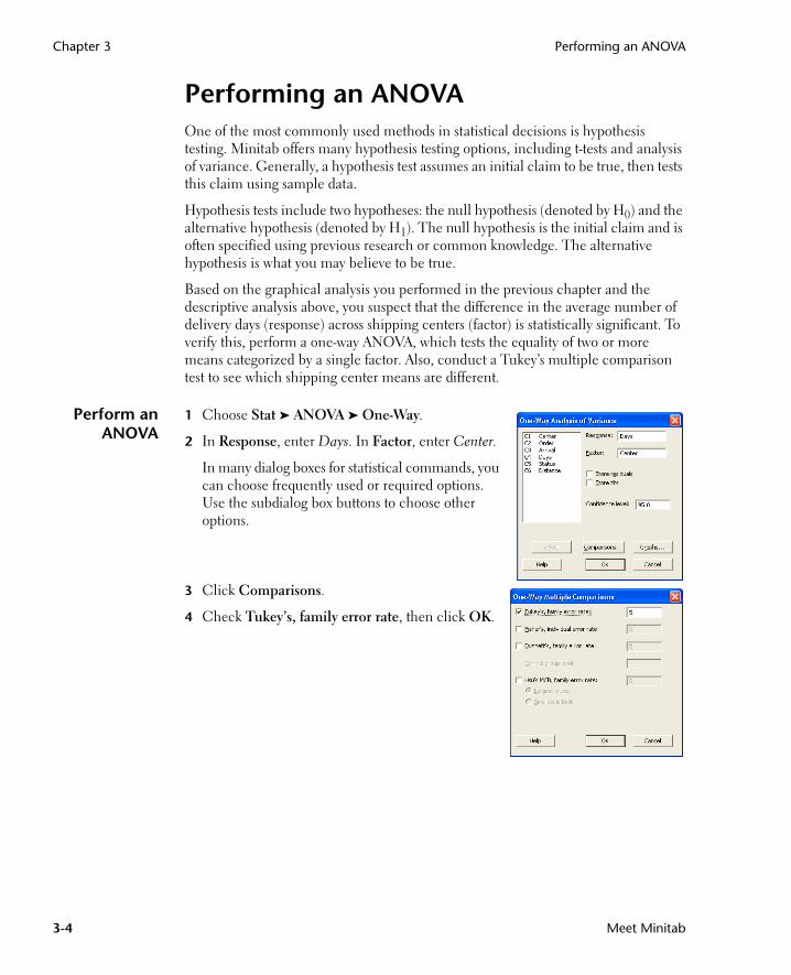
Perform anANOVA
1 Choose Stat ➤ ANOVA ➤ One-Way.
2 In Response, enter Days. In Factor, enter Center.
In many dialog boxes for statistical commands, you can choose frequently used or required options. Use the subdialog box buttons to choose other options.
3 Click Comparisons.
4 Check Tukey’s, family error rate, then click OK.
MeetMinitab.book Page 4 Monday, April 6, 2009 11:25 AM
Performing an ANOVA Analyzing Data
Meet Minitab 3-5
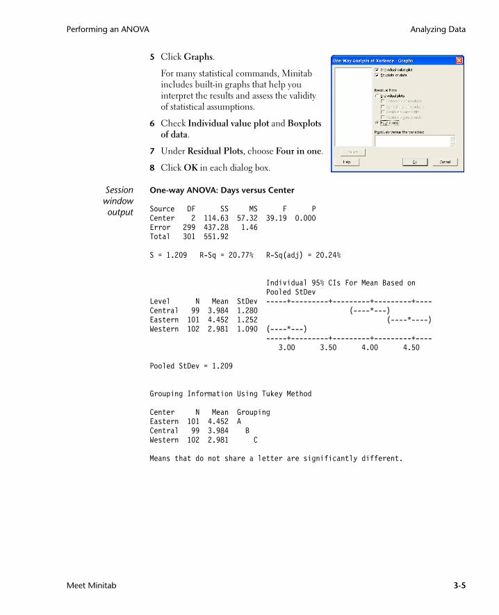
5 Click Graphs.
For many statistical commands, Minitab includes built-in graphs that help you interpret the results and assess the validity of statistical assumptions.
6 Check Individual value plot and Boxplots of data.
7 Under Residual Plots, choose Four in one.
8 Click OK in each dialog box.
Sessionwindowoutput
One-way ANOVA: Days versus Center
Source DF SS MS F PCenter 2 114.63 57.32 39.19 0.000Error 299 437.28 1.46Total 301 551.92
S = 1.209 R-Sq = 20.77% R-Sq(adj) = 20.24%
Individual 95% CIs For Mean Based on Pooled StDevLevel N Mean StDev -----+---------+---------+---------+----Central 99 3.984 1.280 (----*---)Eastern 101 4.452 1.252 (----*----)Western 102 2.981 1.090 (----*---) -----+---------+---------+---------+---- 3.00 3.50 4.00 4.50
Pooled StDev = 1.209
Grouping Information Using Tukey Method
Center N Mean GroupingEastern 101 4.452 ACentral 99 3.984 BWestern 102 2.981 C
Means that do not share a letter are significantly different.
MeetMinitab.book Page 5 Monday, April 6, 2009 11:25 AM

Chapter 3 Performing an ANOVA
3-6 Meet Minitab
Tukey 95% Simultaneous Confidence IntervalsAll Pairwise Comparisons among Levels of Center
Individual confidence level = 98.01%
Center = Central subtracted from:
Center Lower Center Upper ---------+---------+---------+---------+Eastern 0.068 0.468 0.868 (---*---)Western -1.402 -1.003 -0.603 (---*---) ---------+---------+---------+---------+ -1.0 0.0 1.0 2.0
Center = Eastern subtracted from:
Center Lower Center Upper ---------+---------+---------+---------+Western -1.868 -1.471 -1.073 (---*---) ---------+---------+---------+---------+ -1.0 0.0 1.0 2.0
Interpretresults
The decision-making process for a hypothesis test can be based on the probability value (p-value) for the given test.
■ If the p-value is less than or equal to a predetermined level of significance (α-level), then you reject the null hypothesis and claim support for the alternative hypothesis.
■ If the p-value is greater than the α-level, you fail to reject the null hypothesis and cannot claim support for the alternative hypothesis.
In the ANOVA table, the p-value (0.000) provides sufficient evidence that the average delivery time is different for at least one of the shipping centers from the others when α is 0.05. In the individual 95% confidence intervals table, notice that none of the intervals overlap, which supports the theory that the means are statistically different. However, you need to interpret the multiple comparison results to see where the differences exist among the shipping center averages.
Tukey’s test provides grouping information and two sets of multiple comparison intervals. In the grouping table, factor levels within the same group are not significantly different from each other. Each shipping center is in a different group. Therefore, all levels means have significantly different average delivery times.
The Tukey confidence intervals show:
■ Central shipping center mean subtracted from Eastern and Western shipping center means
■ Eastern shipping center mean subtracted from Western center mean
MeetMinitab.book Page 6 Monday, April 6, 2009 11:25 AM

Performing an ANOVA Analyzing Data
Meet Minitab 3-7
The first interval in the first set of the Tukey output is 0.068 to 0.868. That is, the mean delivery time of the Eastern center minus that of the Central center is somewhere between 0.068 and 0.868 days. The Eastern center’s deliveries take longer than the Central center’s deliveries. You similarly interpret the other Tukey test results. The means for all shipping centers differ significantly because all of the confidence intervals exclude zero. Therefore, all the shipping centers have significantly different average delivery times. The Western shipping center has the fastest mean delivery time (2.981 days).
Graphwindowoutput
Interpretresults
The individual value plots and boxplots indicate that the delivery time varies by shipping center, which is consistent with the graphs from the previous chapter. The boxplot for the Eastern shipping center indicates the presence of one outlier (indicated by ∗), which is an order with an unusually long delivery time.
Use residual plots, available with many statistical commands, to check statistical assumptions:
■ Normal probability plot—to detect nonnormality. An approximately straight line indicates that the residuals are normally distributed.
■ Histogram of the residuals—to detect multiple peaks, outliers, and nonnormality. The histogram should be approximately symmetric and bell-shaped.
MeetMinitab.book Page 7 Monday, April 6, 2009 11:25 AM

Chapter 3 Using Minitab’s Project Manager
3-8 Meet Minitab
■ Residuals versus the fitted values—to detect nonconstant variance, missing higher-order terms, and outliers. The residuals should be scattered randomly around zero.
■ Residuals versus order—to detect time-dependence of residuals. The residuals should exhibit no clear pattern.
For the shipping data, the four-in-one residual plots indicate no violations of statistical assumptions. The one-way ANOVA model fits the data reasonably well.
AccessStatGuide
You want more information on how to interpret a one-way ANOVA, particularly Tukey’s multiple comparison test. Minitab StatGuide provides detailed information about the Session and Graph window output for most statistical commands.
1 Place your cursor anywhere in the one-way ANOVA Session window output.
2 Click on the Standard toolbar.
3 You want to learn more about Tukey’s multiple comparison method. In the Contents pane, click Tukey’s method.
4 If you like, use to browse through the one-way ANOVA topics.
5 In the StatGuide window, click to close it.
Save project Save all your work in a Minitab project.
1 Choose File ➤ Save Project As.
2 Navigate to the folder in which you want to save your files.
3 In File name, type My_Stats.MPJ.
4 Click Save.
Using Minitab’s Project ManagerNow you have a Minitab project that contains a worksheet, several graphs, and Session window output from your analyses. The Project Manager helps you navigate, view, and manipulate parts of your Minitab project.
Use the Project Manager to view the statistical analyses you just conducted.
In Minitab, you can display each of the residual plots on a separate page. You can also create a plot of the residuals versus the variables.
For more information about using the StatGuide, see StatGuide on page 10-8.
MeetMinitab.book Page 8 Monday, April 6, 2009 11:25 AM

Using Minitab’s Project Manager Analyzing Data
Meet Minitab 3-9
Open ProjectManager
1 To access the Project Manager, click on the Project Manager toolbar or press [Ctrl]+[I].
You can easily view the Session window output and graphs by choosing from the list in the right pane. You can also use the icons on the Project Manager toolbar to access different output.
For more information, see Project Manager on page 11-3.
View Sessionwindowoutput
You want to review the one-way ANOVA output. To become familiar with the Project Manager toolbar, use the Show Session Folder icon on the toolbar, which opens the Session window.
1 Click on the Project Manager toolbar.
2 Double-click One-way ANOVA: Days versus Center in the left pane.
MeetMinitab.book Page 9 Monday, April 6, 2009 11:25 AM
Chapter 3 Using Minitab’s Project Manager
3-10 Meet Minitab
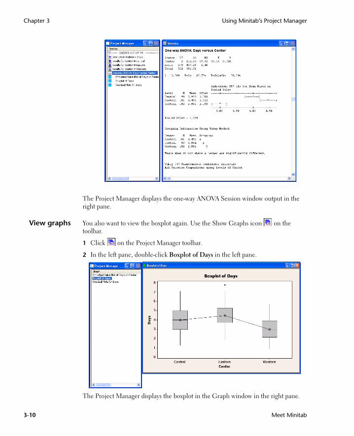
The Project Manager displays the one-way ANOVA Session window output in the right pane.
View graphs You also want to view the boxplot again. Use the Show Graphs icon on the toolbar.
1 Click on the Project Manager toolbar.
2 In the left pane, double-click Boxplot of Days in the left pane.
The Project Manager displays the boxplot in the Graph window in the right pane.
MeetMinitab.book Page 10 Monday, April 6, 2009 11:25 AM

What’s Next Analyzing Data
Meet Minitab 3-11
What’s NextThe descriptive statistics and ANOVA results indicate that the Western center has the fewest late and back orders and the shortest delivery time. In the next chapter, you create a control chart and conduct a capability analysis to investigate whether the Western shipping center’s process is stable over time and is capable of operating within specifications.
MeetMinitab.book Page 11 Monday, April 6, 2009 11:25 AM

Chapter 3 What’s Next
3-12 Meet Minitab
MeetMinitab.book Page 12 Monday, April 6, 2009 11:25 AM

Meet Minitab 4-1
4Assessing Quality
ObjectivesIn this chapter, you:
■ Set options for control charts, page 4-2
■ Create and interpret control charts, page 4-3
■ Update a control chart, page 4-5
■ View subgroup information, page 4-7
■ Add a reference line to a control chart, page 4-7
■ Conduct and interpret a capability analysis, page 4-9
OverviewQuality is the degree to which products or services meet the needs of customers. Common objectives for quality professionals include reducing defect rates, manufacturing products within specifications, and standardizing delivery time.
Minitab offers a wide array of methods to help you evaluate quality in an objective, quantitative way: control charts, quality planning tools, and measurement systems analysis (gage studies), process capability, and reliability/survival analysis. This chapter discusses control charts and process capability.
Features of Minitab control charts include:
■ The ability to choose how to estimate parameters and control limits, as well as display tests for special causes and historical stages.
■ Customizable attributes, such as adding a reference line, changing the scale, and modifying titles. As with other Minitab graphs, you can customize control charts when and after you create them.
MeetMinitab.book Page 1 Monday, April 6, 2009 11:25 AM

Chapter 4 Evaluating Process Stability
4-2 Meet Minitab
Features of process capability commands include:
■ The ability to analyze many data distribution types, such as normal, exponential, Weibull, gamma, Poisson, and binomial.
■ An array of charts that can be used to verify that the process is in control and that the data follow the chosen distribution.
The graphical and statistical analyses conducted in the previous chapter show that the Western shipping center has the fastest delivery time. In this chapter, you determine whether the center’s process is stable (in control) and capable of operating within specifications.
Evaluating Process StabilityUse control charts to track process stability over time and to detect the presence of special causes, which are unusual occurrences that are not a normal part of the process.
Minitab plots a process statistic—such as a subgroup mean, individual observation, weighted statistic, or number of defects—versus a sample number or time. Minitab draws the:
■ Center line at the average of the statistic
■ Upper control limit (UCL) at 3 standard deviations above the center line
■ Lower control limit (LCL) at 3 standard deviations below the center line
For all control charts, you can modify Minitab’s default chart specifications. For example, you can define the estimation method for the process standard deviation, specify the tests for special causes, and display process stages by defining historical stages.
Set optionsfor control
charts
Before you create a control chart for the book shipping data, you want to specify options different from Minitab’s defaults for testing the randomness of the data for all control charts.
The Automotive Industry Action Group (AIAG) suggests using the following guidelines to test for special causes:
■ Test 1: 1 point > 3 standard deviations from center line
■ Test 2: 9 points in a row on the same side of center line
■ Test 3: 6 points in a row, all increasing or all decreasing
For additional information on Minitab’s control charts, go to Control Charts in the Minitab Help index.
MeetMinitab.book Page 2 Monday, April 6, 2009 11:25 AM
Evaluating Process Stability Assessing Quality
Meet Minitab 4-3
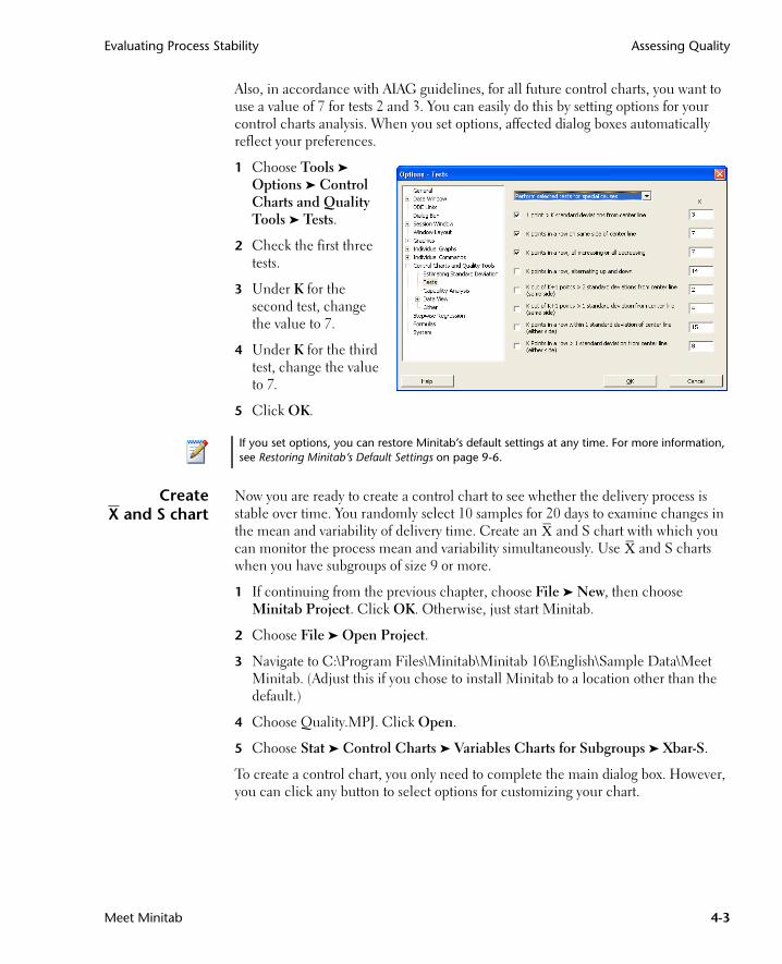
Also, in accordance with AIAG guidelines, for all future control charts, you want to use a value of 7 for tests 2 and 3. You can easily do this by setting options for your control charts analysis. When you set options, affected dialog boxes automatically reflect your preferences.
1 Choose Tools ➤ Options ➤ Control Charts and Quality Tools ➤ Tests.
2 Check the first three tests.
3 Under K for the second test, change the value to 7.
4 Under K for the third test, change the value to 7.
5 Click OK.
CreateX and S chart
Now you are ready to create a control chart to see whether the delivery process is stable over time. You randomly select 10 samples for 20 days to examine changes in the mean and variability of delivery time. Create an and S chart with which you can monitor the process mean and variability simultaneously. Use and S charts when you have subgroups of size 9 or more.
1 If continuing from the previous chapter, choose File ➤ New, then choose Minitab Project. Click OK. Otherwise, just start Minitab.
2 Choose File ➤ Open Project.
3 Navigate to C:\Program Files\Minitab\Minitab 16\English\Sample Data\Meet Minitab. (Adjust this if you chose to install Minitab to a location other than the default.)
4 Choose Quality.MPJ. Click Open.
5 Choose Stat ➤ Control Charts ➤ Variables Charts for Subgroups ➤ Xbar-S.
To create a control chart, you only need to complete the main dialog box. However, you can click any button to select options for customizing your chart.
If you set options, you can restore Minitab’s default settings at any time. For more information, see Restoring Minitab’s Default Settings on page 9-6.
XX
MeetMinitab.book Page 3 Monday, April 6, 2009 11:25 AM
Chapter 4 Evaluating Process Stability
4-4 Meet Minitab
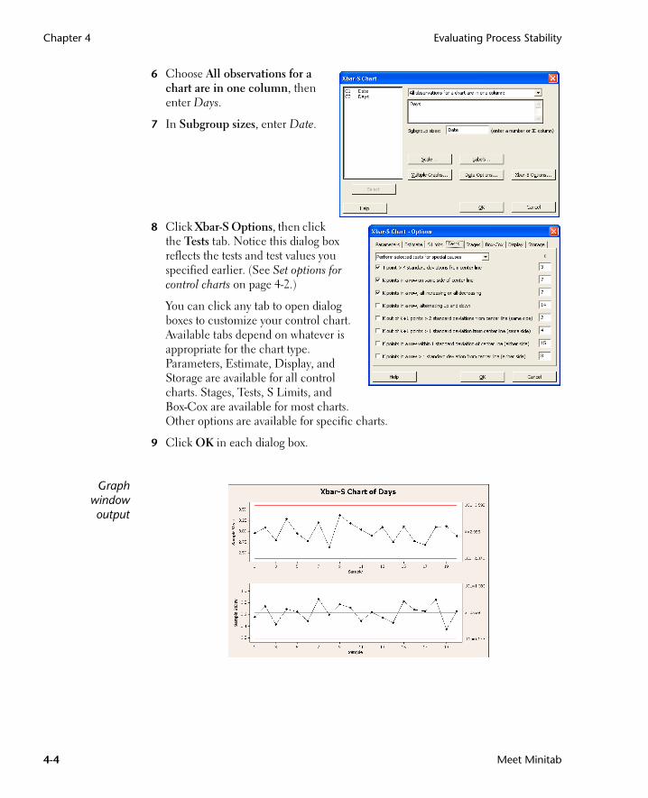
6 Choose All observations for a chart are in one column, then enter Days.
7 In Subgroup sizes, enter Date.
8 Click Xbar-S Options, then click the Tests tab. Notice this dialog box reflects the tests and test values you specified earlier. (See Set options for control charts on page 4-2.)
You can click any tab to open dialog boxes to customize your control chart. Available tabs depend on whatever is appropriate for the chart type. Parameters, Estimate, Display, and Storage are available for all control charts. Stages, Tests, S Limits, and Box-Cox are available for most charts. Other options are available for specific charts.
9 Click OK in each dialog box.
Graphwindowoutput
MeetMinitab.book Page 4 Monday, April 6, 2009 11:25 AM

Evaluating Process Stability Assessing Quality
Meet Minitab 4-5
InterpretX and S chart
The data points for the Western shipping center fall within the bounds of the control limits, and do not display any nonrandom patterns. Therefore, the process mean and process standard deviation appear to be in control (stable). The mean ( ), is 2.985, and the average standard deviation ( ) is 0.629.
Updatecontrol chart
Graph updating allows you to update a graph when the data change without re-creating the graph. Graph updating is available for all graphs in the Graph menu (except Stem-and-Leaf) and all control charts.
After creating the and S chart, the Western shipping center manager gives you more data collected on 3/23/2009. Add the data to the worksheet and update the control chart.
Add the data to the worksheet
You need to add both date/time data to C1 and numeric data to C2.
1 Click the Data window to make it active.
2 Place your cursor in any cell in C1, then press [End] to go to the bottom of the worksheet.
3 To add the date 3/23/2009 to rows 201–210:
■ First, type 3/23/2009 in row 201 in C1.
■ Then, select the cell containing 3/23/2009, place the cursor over the Autofill handle in the lower-right corner of the highlighted cell. When the mouse is over the handle, a cross symbol (+) appears. Press [Ctrl] and drag the cursor to row 210 to fill the cells with the repeated date value. When you hold [Ctrl] down, a superscript cross appears above the Autofill cross symbol (++), indicating that repeated, rather than sequential, values will be added to the cells.
4 Add the following data to C2, starting in row 201:
3.60 2.40 2.80 3.21 2.40 2.75 2.79 3.40 2.58 2.50
S
X
MeetMinitab.book Page 5 Monday, April 6, 2009 11:25 AM

Chapter 4 Evaluating Process Stability
4-6 Meet Minitab
If the data entry arrow is facing downward, pressing [Enter] moves the cursor to the next cell down.
5 Verify that you entered the data correctly.
Update the control chart
1 Right-click the and S chart and choose Update Graph Now.
Graphwindowoutput
The and S chart now includes the new subgroup. The mean ( = 2.978) and standard deviation ( = 0.6207) have changed slightly, but the process still appears to be in control.
Data entry arrow
X
XS
To update all graphs and control charts automatically:1 Choose Tools ➤ Options ➤ Graphics ➤ Other Graphics Options.2 Check On creation, set graph to update automatically when data change.
MeetMinitab.book Page 6 Monday, April 6, 2009 11:25 AM

Evaluating Process Stability Assessing Quality
Meet Minitab 4-7
Viewsubgroup
information
As with any Minitab graph, when you move your mouse over the points in a control chart, you see various information about the data.
You want to find out the mean of sample 9, the subgroup with the largest mean.
1 Move your mouse over the data point for sample 9.
Graphwindowoutput
Interpretresults
The data tip shows that sample 9 has a mean delivery time of 3.369 days.
Addreference line
A goal for the online bookstore is for all customers to receive their orders in 3.33 days (80 hours) on average, so you want to compare the average delivery time for the Western shipping center to this target. You can show the target level on the chart by adding a reference line.
1 Right-click the chart (the top chart), and choose Add ➤ Reference Lines.
2 In Show reference lines at Y values, type 3.33.
3 Click OK.
X
X
MeetMinitab.book Page 7 Monday, April 6, 2009 11:25 AM

Chapter 4 Evaluating Process Capability
4-8 Meet Minitab
Graphwindowoutput
Interpretresults
The center line ( ) is well below the reference line, indicating that, on average, the Western shipping center delivers books faster than the target of 3.33 days. Only subgroup 9 has a delivery time that falls above the reference line (> 3.33).
Evaluating Process CapabilityAfter you determine that a process is in statistical control, you want to know whether the process is capable—does it meet specifications and produce “good” parts or results? You determine capability by comparing the spread of the process variation to the width of the specification limits. If the process is not in control before you assess its capability, you may get incorrect estimates of process capability.
In Minitab, you can assess process capability graphically by drawing capability histograms and capability plots. These graphs help you assess the distribution of the data and verify that the process is in control. Capability indices, or statistics, are a simple way of assessing process capability. Because process information is reduced to a single number, you can use capability statistics to compare the capability of one process to another. Minitab offers capability analysis for many distribution types, including normal, exponential, Weibull, gamma, Poisson, and binomial.
For more information on process capability, go to Process Capability in the Minitab Help index.
MeetMinitab.book Page 8 Monday, April 6, 2009 11:25 AM

Evaluating Process Capability Assessing Quality
Meet Minitab 4-9
Conductcapability
analysis
Now that you know the delivery process is in control, conduct a capability analysis to determine whether the book delivery process is within specification limits and results in acceptable delivery times. The target value of the delivery process is 3.33 days. The upper specification limit (USL) is 6 (an order that is received after 6 days is considered late); no lower specification limit (LSL) is identified. The distribution is approximately normal, so you can use a normal capability analysis.
1 Choose Stat ➤ Quality Tools ➤ Capability Analysis ➤ Normal.
2 Under Data are arranged as, choose Single column. Enter Days.
3 In Subgroup size, enter Date.
4 In Upper spec, type 6.
5 Click Options. In Target (adds Cpm to table), type 3.33.
As with other Minitab commands, you can modify a capability analysis either by specifying information in the main dialog box or by clicking one of the subdialog box buttons.
6 Click OK in each dialog box.
Graphwindowoutput
MeetMinitab.book Page 9 Monday, April 6, 2009 11:25 AM

Chapter 4 What’s Next
4-10 Meet Minitab
Interpretresults
All the potential and overall capability statistics are larger than 1.33 (a generally accepted minimum value), indicating the Western shipping center’s process is capable and, therefore, delivers orders in an acceptable amount of time.
The Cpm value (the ratio of the specification spread, USL – LSL, to the square root of the mean squared deviation from the target value) is 1.22, which indicates that the process does not meet the target value. The chart with the reference line shows that the process average fell below the target value, indicating favorable results. You conclude that customers, on average, are getting their orders sooner than the goal of 3.33 days.
Save project Save all of your work in a Minitab project.
1 Choose File ➤ Save Project As.
2 Navigate to the folder in which you want to save your files.
3 In File name, type My_Quality.MPJ.
4 Click Save.
What’s NextThe quality analysis indicates that the Western shipping center’s process is in control and is capable of meeting specification limits. In the next chapter, you design an experiment and analyze the results to investigate ways to further improve the order and delivery process at the Western shipping center.
X
For more information on how to interpret capability analyses, go to the Capability Analysis topics in the StatGuide.
MeetMinitab.book Page 10 Monday, April 6, 2009 11:25 AM

Meet Minitab 5-1
5Designing an Experiment
ObjectivesIn this chapter, you:
■ Become familiar with designed experiments in Minitab, page 5-1
■ Create a factorial design, page 5-2
■ View a design and enter data in the worksheet, page 5-5
■ Analyze a design and interpret results, page 5-6
■ Create and interpret main effects and interaction plots, page 5-9
OverviewDesign of experiments (DOE) capabilities provide a method for simultaneously investigating the effects of multiple variables on an output variable (response). These experiments consist of a series of runs, or tests, in which purposeful changes are made to input variables or factors, and data are collected at each run. Quality professionals use DOE to identify the process conditions and product components that influence quality and then determine the input variable (factor) settings that maximize results.
Minitab offers four types of designed experiments: factorial, response surface, mixture, and Taguchi (robust). The steps you follow in Minitab to create, analyze, and graph an experimental design are similar for all design types. After you conduct the experiment and enter the results, Minitab provides several analytical and graphing tools to help you understand the results. While this chapter demonstrates the typical steps for creating and analyzing a factorial design, you can apply these steps to any design you create in Minitab.
MeetMinitab.book Page 1 Monday, April 6, 2009 11:25 AM

Chapter 5 Creating an Experimental Design
5-2 Meet Minitab
Features of Minitab DOE commands include:
■ Catalogs of experimental designs from which you can choose, to make creating a design easier
■ Automatic creation and storage of your design once you have specified its properties
■ Ability to display and store diagnostic statistics, to help you interpret the results
■ Graphs that assist you in interpreting and presenting the results
In this chapter, you want to further improve the amount of time it takes to get orders to customers from the Western shipping center. After evaluating many potentially important factors, you decide to investigate two factors that may decrease the time to prepare an order for shipment: the order processing system and packing procedure.
The Western center is experimenting with a new order processing system and you want to determine if it will speed up order preparation. The center also has two different packing procedures and you want to investigate which one is more efficient. You decide to conduct a factorial experiment to find out which combination of factors results in the shortest time to prepare an order for shipment. The results of this experiment will help you make decisions about the order processing system and packing procedures used in the shipping center.
Creating an Experimental Design
Before you can enter or analyze measurement data in Minitab, you must first create an experimental design and store it in the worksheet. Depending on the requirements of your experiment, you can choose from a variety of designs. Minitab helps you select a design by providing a list of all the available designs. Once you have chosen the design and its features, Minitab automatically creates the design and stores it in the worksheet for you.
Select design You want to create a factorial design to examine the relationship between two factors, order processing system and packing procedure, and the time it takes to prepare an order for shipping.
1 If continuing from the previous chapter, choose File ➤ New, then choose Minitab Project. Click OK. Otherwise, just start Minitab.
For more information on the types of designs that Minitab offers, go to DOE in the Minitab Help index.
MeetMinitab.book Page 2 Monday, April 6, 2009 11:25 AM
Creating an Experimental Design Designing an Experiment
Meet Minitab 5-3
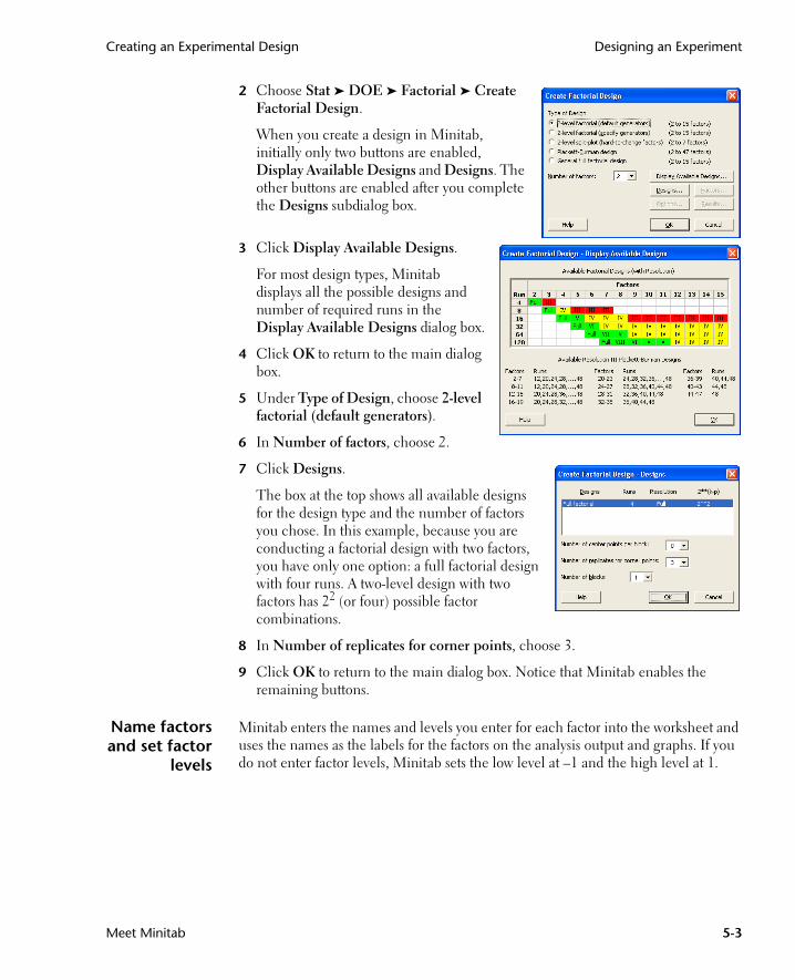
2 Choose Stat ➤ DOE ➤ Factorial ➤ Create Factorial Design.
When you create a design in Minitab, initially only two buttons are enabled, Display Available Designs and Designs. The other buttons are enabled after you complete the Designs subdialog box.
3 Click Display Available Designs.
For most design types, Minitab displays all the possible designs and number of required runs in the Display Available Designs dialog box.
4 Click OK to return to the main dialog box.
5 Under Type of Design, choose 2-level factorial (default generators).
6 In Number of factors, choose 2.
7 Click Designs.
The box at the top shows all available designs for the design type and the number of factors you chose. In this example, because you are conducting a factorial design with two factors, you have only one option: a full factorial design with four runs. A two-level design with two factors has 22 (or four) possible factor combinations.
8 In Number of replicates for corner points, choose 3.
9 Click OK to return to the main dialog box. Notice that Minitab enables the remaining buttons.
Name factorsand set factor
levels
Minitab enters the names and levels you enter for each factor into the worksheet and uses the names as the labels for the factors on the analysis output and graphs. If you do not enter factor levels, Minitab sets the low level at –1 and the high level at 1.
MeetMinitab.book Page 3 Monday, April 6, 2009 11:25 AM

Chapter 5 Creating an Experimental Design
5-4 Meet Minitab
1 Click Factors.
2 Click the first row of the Name column to change the name of the first factor. Then, use the arrow keys to navigate within the table, moving across rows or down columns. In the row for:
■ Factor A, type OrderSystem in Name, New in Low, and Current in High. Under Type, choose Text.
■ Factor B, type Pack in Name, A in Low, and B in High. Under Type, choose Text.
3 Click OK to return to the main dialog box.
Randomizeand store
design
By default, Minitab randomizes the run order of all design types, except Taguchi designs. Randomization helps to ensure that the model meets certain statistical assumptions and can also help reduce the effects of factors not included in the study.
Setting the base for the random data generator ensures you obtain the same run order every time you create the design. While you usually would not do this in practice, setting the base gives the same run order that is used in this example.
1 Click Options.
2 In Base for random data generator, type 9.
3 Make sure Store design in worksheet is checked. Click OK in each dialog box.
MeetMinitab.book Page 4 Monday, April 6, 2009 11:25 AM

Viewing the Design Designing an Experiment
Meet Minitab 5-5
Viewing the DesignEvery time you create a design, Minitab stores design information and factors in worksheet columns. Open the Data window to see the structure of a typical design. You can also open the worksheet DOE.MTW in the Meet Minitab data folder, which includes the design and the response data.
View design 1 Choose Window ➤ Worksheet 1.
The RunOrder column (C2), which is randomly determined, indicates the order in which you should collect data. If you do not randomize a design, the StdOrder and RunOrder columns are the same.
In this example, because you did not add center points or block the design, Minitab sets all the values in C3 and C4 to 1. The factors are stored in columns C5 and C6, labeled OrderSystem and Pack. Because you entered the factor levels in the Factors subdialog box, you see the actual levels in the worksheet.
Entering DataAfter you conduct the experiment and collect the data, you can enter the data into the worksheet. The characteristic you measure is called a response.
In this example, you measure the number of hours needed to prepare an order for shipment. You obtained the following data from the experiment:
14.72 9.62 13.81 7.97 12.52 13.78 14.64 9.41 13.89 13.89 12.57 14.06
You can use Stat ➤ DOE ➤ Display Design to switch back and forth between a random and standard order display, and between a coded and uncoded display in the worksheet.
To change the factor settings or names, use Stat ➤ DOE ➤ Modify Design. If you only need to change the factor names, you can type them directly in the Data window.
MeetMinitab.book Page 5 Monday, April 6, 2009 11:25 AM

Chapter 5 Analyzing the Design
5-6 Meet Minitab
Enter datainto
worksheet
1 In the Data window, click the column name cell of C7 and type Hours.
2 Type the observed hours listed above into the Hours column of the Data window.
You can enter data in any columns except in those containing design information. You can also enter multiple responses for an experiment, one per column.
Analyzing the DesignNow that you have created a design and collected the response data, you can fit a model to the data and generate graphs to evaluate the effects. Use the results from the fitted model and graphs to see which factors are important for reducing the number of hours needed to prepare an order for shipment.
Fit a model Because you have created and stored a factorial design, Minitab enables the DOE ➤ Factorial menu commands Analyze Factorial Design and Factorial Plots. At this point, you can fit a model or generate plots, depending on the design. In this example, you fit the model first.
1 Choose Stat ➤ DOE ➤ Factorial ➤ Analyze Factorial Design.
2 In Responses, enter Hours.
You must enter a response column before you can open the subdialog boxes.
Print a data collection form by choosing File ➤ Print Worksheet and making sure Print Grid Lines is checked. Use this form to record measurements while you conduct the experiment.
MeetMinitab.book Page 6 Monday, April 6, 2009 11:25 AM

Analyzing the Design Designing an Experiment
Meet Minitab 5-7
3 Click Terms. Check to make sure that A: OrderSystem, B: Pack and AB are in the Selected Terms box.
When analyzing a design, always use the Terms subdialog box to select the terms to include in the model. You can add or remove factors and interactions by using the arrow buttons. Use the check boxes to include blocks and center points in the model.
4 Click OK.
5 Click Graphs.
6 Under Effects Plots, check Normal and Pareto.
Effects plots are only available in factorial designs. Residual plots, helpful in checking model assumptions, can be displayed for all design types.
7 Click OK in each dialog box.
Identifyimportant
effects
You can use both the Session window output and the two effects plots to determine which effects are important to your process. First, look at the Session window output.
Sessionwindowoutput
Factorial Fit: Hours versus OrderSystem, Pack
Estimated Effects and Coefficients for Hours (coded units)
Term Effect Coef SE Coef T PConstant 12.573 0.1929 65.20 0.000OrderSystem 3.097 1.548 0.1929 8.03 0.000Pack -2.320 -1.160 0.1929 -6.01 0.000OrderSystem*Pack 1.730 0.865 0.1929 4.49 0.002
S = 0.668069 PRESS = 8.0337R-Sq = 93.79% R-Sq(pred) = 86.02% R-Sq(adj) = 91.46%
MeetMinitab.book Page 7 Monday, April 6, 2009 11:25 AM
Chapter 5 Analyzing the Design
5-8 Meet Minitab
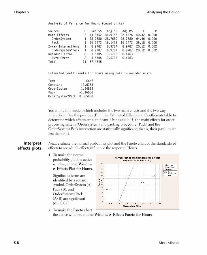
Analysis of Variance for Hours (coded units)
Source DF Seq SS Adj SS Adj MS F PMain Effects 2 44.9152 44.9152 22.4576 50.32 0.000 OrderSystem 1 28.7680 28.7680 28.7680 64.46 0.000 Pack 1 16.1472 16.1472 16.1472 36.18 0.0002-Way Interactions 1 8.9787 8.9787 8.9787 20.12 0.002 OrderSystem*Pack 1 8.9787 8.9787 8.9787 20.12 0.002Residual Error 8 3.5705 3.5705 0.4463 Pure Error 8 3.5705 3.5705 0.4463Total 11 57.4645
Estimated Coefficients for Hours using data in uncoded units
Term CoefConstant 12.5733OrderSystem 1.54833Pack -1.16000OrderSystem*Pack 0.865000
You fit the full model, which includes the two main effects and the two-way interaction. Use the p-values (P) in the Estimated Effects and Coefficients table to determine which effects are significant. Using α = 0.05, the main effects for order processing system (OrderSystem) and packing procedure (Pack) and the OrderSystem∗Pack interaction are statistically significant; that is, their p-values are less than 0.05.
Interpreteffects plots
Next, evaluate the normal probability plot and the Pareto chart of the standardized effects to see which effects influence the response, Hours.
1 To make the normal probability plot the active window, choose Window ➤ Effects Plot for Hours.
Significant terms are identified by a square symbol. OrderSystem (A), Pack (B), and OrderSystem∗Pack (A∗B) are significant (α = 0.05).
2 To make the Pareto chart the active window, choose Window ➤ Effects Pareto for Hours.
MeetMinitab.book Page 8 Monday, April 6, 2009 11:25 AM

Drawing Conclusions Designing an Experiment
Meet Minitab 5-9
Minitab displays the absolute value of the effects on the Pareto chart. Any effects that extend beyond the reference line are significant at the default level of 0.05.
OrderSystem (A), Pack (B) and OrderSystem∗Pack (A∗B) are all significant (α = 0.05).
Drawing Conclusions
Displayfactorial plots
Minitab provides design-specific graphs you can use to interpret your results.
In this example, you generate two factorial plots that enable you to visualize the effects—a main effects plot and an interaction plot.
1 Choose Stat ➤ DOE ➤ Factorial ➤ Factorial Plots.
2 Check Main Effects Plot, then click Setup.
3 In Responses, enter Hours.
4 Select the terms you want to plot:
■ Click A:OrderSystem under Available. Then click to move A:OrderSystem factor to Selected.
■ Repeat these actions to move B:Pack to Selected. Click OK.
5 Check Interaction Plot, then click Setup.
6 Repeat steps 3 and 4.
MeetMinitab.book Page 9 Monday, April 6, 2009 11:25 AM

Chapter 5 Drawing Conclusions
5-10 Meet Minitab
7 Click OK in each dialog box.
Evaluate plots Examine the plot that shows the effect of using the new versus current order processing system, or using packing procedure A versus B. These one-factor effects are called main effects.
1 Choose Window ➤ Main Effects Plot for Hours to make the main effects plot active.
The order processing system and packing procedure have a similar effect on order preparation time. That is, the line connecting the mean responses for the new and current order processing system has a slope similar to slope of the line connecting the mean response for packing procedure A and packing procedure B. The plot also indicates that orders using:
■ The new order processing system took less time than orders that used the current order processing system.
■ Packing procedures B took less time than orders that used packing procedure A
If there were no significant interactions between the factors, a main effects plot would adequately describe where you can get the biggest payoff for changes to your process. Because the interaction in this example is significant, you should next examine the interaction plot. A significant interaction between two factors can affect the interpretation of the main effects.
This point shows the mean of all runs using the current order processing system.
This point shows the mean of all runs using the new order processing system.
This line shows the mean of all the response (Hours) in the experiment.
MeetMinitab.book Page 10 Monday, April 6, 2009 11:25 AM

Drawing Conclusions Designing an Experiment
Meet Minitab 5-11
2 Choose Window ➤ Interaction Plot for Hours to make the interaction plot active.
An interaction plot shows the impact that changing the settings of one factor has on another factor. Because an interaction can magnify or diminish main effects, evaluating interactions is extremely important.
The plot shows that book orders processed with the new order processing system and packing procedure B took the fewest hours to prepare (about 9 hours). Orders processed with the current order processing system and packing procedure A took the longest to prepare (about 14.5 hours). Because the slope of the line for the new order processing system is steeper, you conclude that the packing procedure has a greater effect when the new order processing system is used versus the current order processing system.
Based on the results of the experiment, you recommend that the Western shipping center use the new order processing system and packing procedure B to speed up the book shipping process.
Save Project 1 Choose File ➤ Save Project As.
2 Navigate to the folder in which you want to save your files.
3 In File name, enter My_DOE.MPJ.
4 Click Save.
This point is the mean time required to prepare packages using the new order processing system and packing procedure A.
This legend displays the levels of the first factor (OrderSystem).
The horizontal scale (x-axis) shows the levels of the second factor (Pack).
The vertical scale (y-axis) is in units of the response (Hours).
MeetMinitab.book Page 11 Monday, April 6, 2009 11:25 AM
Chapter 5 What’s Next
5-12 Meet Minitab
What’s NextThe factorial experiment indicates you can decrease the time it takes to prepare orders at the Western shipping center by using the new order processing system and packing procedure B. In the next chapter, you learn how to use command language and create and run Execs to quickly rerun an analysis when new data are collected.
MeetMinitab.book Page 12 Monday, April 6, 2009 11:25 AM
Meet Minitab 6-1
6Using Session Commands
ObjectivesIn this chapter, you:
■ Enable and type session commands, page 6-2
■ Conduct an analysis using session commands, page 6-3
■ Rerun a series of session commands with Command Line Editor, page 6-5
■ Create and run an Exec, page 6-7
OverviewEach menu command has a corresponding session command. Session commands consist of a main command and, in most cases, one or more subcommands. Commands are usually easy-to-remember words, such as PLOT, CHART, or SORT. Both main commands and subcommands can be followed by a series of arguments, which can be columns, constants, or matrices, text strings, or numbers.
Session commands can be:
■ Typed into the Session window or the Command Line Editor.
■ Copied from the History folder to the Command Line Editor. (When you use menu commands, Minitab generates and stores the corresponding session commands in the History folder.)
■ Copied and saved in a file called an Exec, which can be reexecuted and shared with others or used in future sessions.
MeetMinitab.book Page 1 Monday, April 6, 2009 11:25 AM

Chapter 6 Enabling and Typing Commands
6-2 Meet Minitab
Use session commands to quickly rerun an analysis in current or future sessions or as an alternative to menu commands. Some users find session commands quicker to use than menu commands once they become familiar with them.
The Western shipping center continuously collects and analyzes shipping time when new data are available. In Chapter 4, Assessing Quality, you conducted a capability analysis on data from March. In this chapter, you conduct a capability analysis on data from April using session commands.
Enabling and Typing CommandsOne way to use session commands is to directly type the commands and subcommands at the command prompt in the Session window. However, Minitab does not display the command prompt by default. To enter commands directly into the Session window, you must enable this prompt.
Enablesession
commands
1 If continuing from the previous chapter, choose File ➤ New, then choose Minitab Project and click OK. Otherwise, just start Minitab.
2 Choose File ➤ Open Worksheet.
3 Click Look in Minitab Sample Data folder, near the bottom of the dialog box.
4 In the Sample Data folder, double-click Meet Minitab, then choose SessionCommands.MTW. Click Open.
5 Click the Session window to make it active.
6 Choose Editor ➤ Enable Commands. A check appears next to the menu item.
To learn more about session commands, choose Help ➤ Help, then click Session Commands under References.
To change the default options and enable session commands for all future sessions:1 Choose Tools ➤ Options ➤ Session Window ➤ Submitting Commands.2 Under Command Language, click Enable.
MeetMinitab.book Page 2 Monday, April 6, 2009 11:25 AM
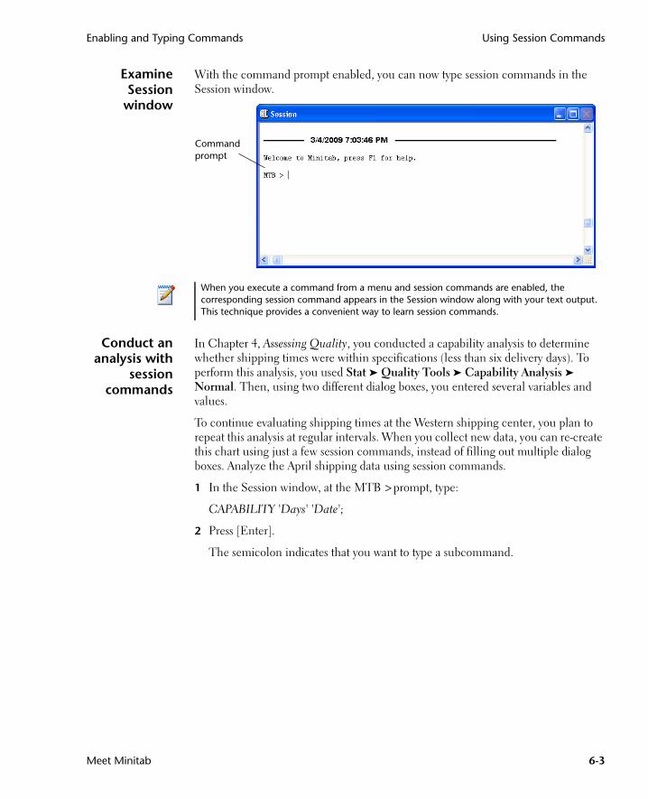
Enabling and Typing Commands Using Session Commands
Meet Minitab 6-3
ExamineSession
window
With the command prompt enabled, you can now type session commands in the Session window.
Conduct ananalysis with
sessioncommands
In Chapter 4, Assessing Quality, you conducted a capability analysis to determine whether shipping times were within specifications (less than six delivery days). To perform this analysis, you used Stat ➤ Quality Tools ➤ Capability Analysis ➤ Normal. Then, using two different dialog boxes, you entered several variables and values.
To continue evaluating shipping times at the Western shipping center, you plan to repeat this analysis at regular intervals. When you collect new data, you can re-create this chart using just a few session commands, instead of filling out multiple dialog boxes. Analyze the April shipping data using session commands.
1 In the Session window, at the MTB > prompt, type:
CAPABILITY 'Days' 'Date';
2 Press [Enter].
The semicolon indicates that you want to type a subcommand.
Command prompt
When you execute a command from a menu and session commands are enabled, the corresponding session command appears in the Session window along with your text output. This technique provides a convenient way to learn session commands.
MeetMinitab.book Page 3 Monday, April 6, 2009 11:25 AM

Chapter 6 Enabling and Typing Commands
6-4 Meet Minitab
Notice that the MTB > prompt becomes SUBC>, allowing you to add subcommands for the various options used in the earlier capability analysis.
3 At the SUBC> prompt, type:
USPEC 6;
4 Press [Enter].
5 At the SUBC> prompt, type:
TARGET 3.33.
6 Press [Enter].
The period indicates the end of a command sequence.
Minitab displays the capability analysis for the April shipping data.
Subcommand prompt
For more information on session commands, including command and subcommand syntax, type Help at the command prompt followed by the first four letters of the command name. For general information on syntax notation, go to Help ➤ Help, then click Session Commands under References. Go to Notation for session commands in the Session Command Help index.
MeetMinitab.book Page 4 Monday, April 6, 2009 11:25 AM
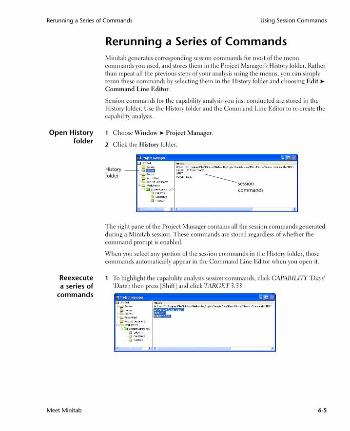
Rerunning a Series of Commands Using Session Commands
Meet Minitab 6-5
Rerunning a Series of CommandsMinitab generates corresponding session commands for most of the menu commands you used, and stores them in the Project Manager’s History folder. Rather than repeat all the previous steps of your analysis using the menus, you can simply rerun these commands by selecting them in the History folder and choosing Edit ➤ Command Line Editor.
Session commands for the capability analysis you just conducted are stored in the History folder. Use the History folder and the Command Line Editor to re-create the capability analysis.
Open Historyfolder
1 Choose Window ➤ Project Manager.
2 Click the History folder.
The right pane of the Project Manager contains all the session commands generated during a Minitab session. These commands are stored regardless of whether the command prompt is enabled.
When you select any portion of the session commands in the History folder, those commands automatically appear in the Command Line Editor when you open it.
Reexecutea series of
commands
1 To highlight the capability analysis session commands, click CAPABILITY 'Days' 'Date'; then press [Shift] and click TARGET 3.33.
session commands
History folder
MeetMinitab.book Page 5 Monday, April 6, 2009 11:25 AM

Chapter 6 Repeating Analyses with Execs
6-6 Meet Minitab
2 Choose Edit ➤ Command Line Editor.
3 Click Submit Commands.
Graphwindowoutput
You have re-created the capability analysis in just a few simple steps.
Repeating Analyses with ExecsAn Exec is a text file containing a series of Minitab commands. To repeat an analysis without using menu commands or typing session commands, save the commands as an Exec and then run the Exec.
If you edit a graph or a control chart, Minitab does not automatically generate session commands for the changes made. However, you can generate the session commands, including all editing changes, by using:
■ Editor ➤ Copy Command Language, which copies the commands to the Clipboard.
■ Editor ➤ Duplicate Graph, which re-creates the graph and stores the session commands in the History folder.
For more information on Copy Command Language and Duplicate Graph, go to Editor menu and choose the Graph window subentry in the Minitab Help index.
MeetMinitab.book Page 6 Monday, April 6, 2009 11:25 AM
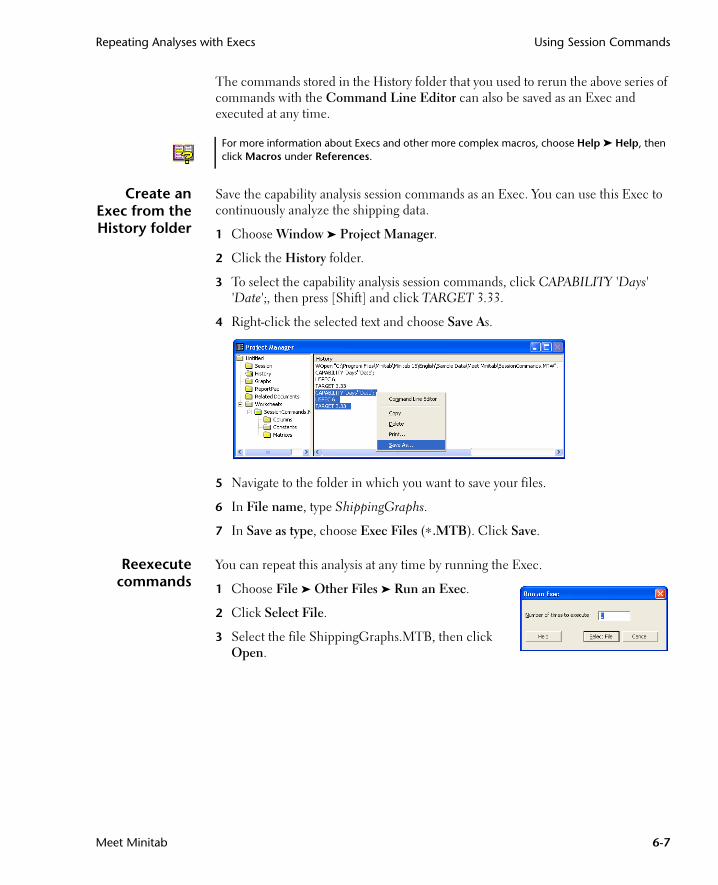
Repeating Analyses with Execs Using Session Commands
Meet Minitab 6-7
The commands stored in the History folder that you used to rerun the above series of commands with the Command Line Editor can also be saved as an Exec and executed at any time.
Create anExec from theHistory folder
Save the capability analysis session commands as an Exec. You can use this Exec to continuously analyze the shipping data.
1 Choose Window ➤ Project Manager.
2 Click the History folder.
3 To select the capability analysis session commands, click CAPABILITY 'Days' 'Date';, then press [Shift] and click TARGET 3.33.
4 Right-click the selected text and choose Save As.
5 Navigate to the folder in which you want to save your files.
6 In File name, type ShippingGraphs.
7 In Save as type, choose Exec Files (∗.MTB). Click Save.
Reexecutecommands
You can repeat this analysis at any time by running the Exec.
1 Choose File ➤ Other Files ➤ Run an Exec.
2 Click Select File.
3 Select the file ShippingGraphs.MTB, then click Open.
For more information about Execs and other more complex macros, choose Help ➤ Help, then click Macros under References.
MeetMinitab.book Page 7 Monday, April 6, 2009 11:25 AM
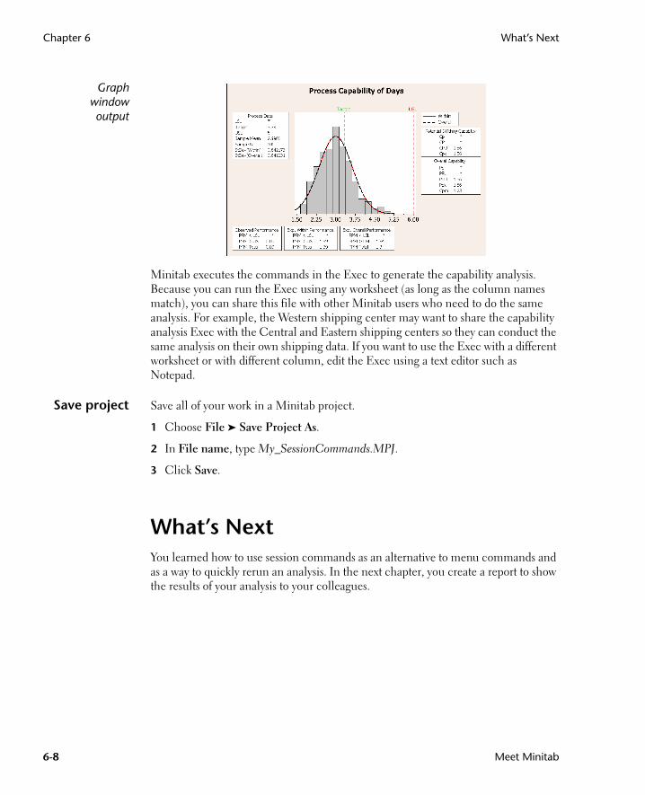
Chapter 6 What’s Next
6-8 Meet Minitab
Graphwindowoutput
Minitab executes the commands in the Exec to generate the capability analysis. Because you can run the Exec using any worksheet (as long as the column names match), you can share this file with other Minitab users who need to do the same analysis. For example, the Western shipping center may want to share the capability analysis Exec with the Central and Eastern shipping centers so they can conduct the same analysis on their own shipping data. If you want to use the Exec with a different worksheet or with different column, edit the Exec using a text editor such as Notepad.
Save project Save all of your work in a Minitab project.
1 Choose File ➤ Save Project As.
2 In File name, type My_SessionCommands.MPJ.
3 Click Save.
What’s NextYou learned how to use session commands as an alternative to menu commands and as a way to quickly rerun an analysis. In the next chapter, you create a report to show the results of your analysis to your colleagues.
MeetMinitab.book Page 8 Monday, April 6, 2009 11:25 AM

Meet Minitab 7-1
7Generating a Report
ObjectivesIn this chapter, you:
■ Add a graph to the ReportPad, page 7-2
■ Add Session window output to the ReportPad, page 7-3
■ Edit in the ReportPad, page 7-5
■ Save and view a report, page 7-6
■ Copy the ReportPad contents to a word processor, page 7-7
■ Edit a Minitab graph in another application, page 7-7
■ Send output to Microsoft PowerPoint, page 7-10
OverviewMinitab has several tools to help you create reports:
■ ReportPad in the Project Manager, to which you can add Minitab-generated results throughout your sessions
■ Copy to Word Processor, which enables you to easily copy content from the ReportPad to a word processor
■ Embedded Graph Editor, for editing graphs with Minitab after you have copied them to other applications
■ Send To Microsoft Word or PowerPoint, which enables you to send Session window output and graphs directly to Word or PowerPoint
To show your colleagues the shipping data analysis results, you want to prepare a report that includes various elements from your Minitab sessions.
MeetMinitab.book Page 1 Monday, April 6, 2009 11:25 AM
Chapter 7 Using the ReportPad
7-2 Meet Minitab
Using the ReportPadThroughout Meet Minitab, you performed several analyses and you want to share the results with colleagues. Minitab’s Project Manager contains a folder, called the ReportPad, in which you can create simple reports.
The ReportPad acts as a simple text editor (like Notepad), from which you can quickly print or save in RTF (rich text) or HTML (Web) format. In ReportPad, you can:
■ Store Minitab results and graphs in a single document
■ Add comments and headings
■ Rearrange your output
■ Change font sizes
■ Print entire output from an analysis
■ Create Web-ready reports
Add graph toReportPad
You can add components to ReportPad by right-clicking on a graph or Session window output, then choosing Append to Report. In addition, text and graphs from other applications can be copied and pasted into Minitab’s ReportPad.
Add the histogram with fits and groups you created in Chapter 2, Graphing Data, to the ReportPad.
1 If continuing from the previous chapter, choose File ➤ New, then choose Minitab Project. Click OK. Otherwise, just start Minitab.
2 Choose File ➤ Open Project.
3 Navigate to C:\Program Files\Minitab\Minitab 16\English\Sample Data\Meet Minitab. (Adjust this if you chose to install Minitab to a location other than the default.)
4 Choose Reports.MPJ. Click Open.
5 Choose Window ➤ Histogram of Days.
MeetMinitab.book Page 2 Monday, April 6, 2009 11:25 AM

Using the ReportPad Generating a Report
Meet Minitab 7-3
6 Right-click anywhere in the graph region, then choose Append Graph to Report.
7 Choose Window ➤ Project Manager.
8 Click the ReportPad folder. The histogram has been added to the ReportPad.
Add Sessionwindow
output toReportPad
You also can add Session window output to the ReportPad. In Chapter 3, Analyzing Data, you displayed descriptive statistics for the three regional shipping centers. Add the output for the three centers to the ReportPad.
1 Choose Window ➤ Session.
Graph region
MeetMinitab.book Page 3 Monday, April 6, 2009 11:25 AM

Chapter 7 Using the ReportPad
7-4 Meet Minitab
2 In the Session window, click in the output for Results for Center = Central. Then right-click and choose Append Section to Report. The section of output Minitab appends is delineated by the output titles (which are in bold text).
3 Repeat the steps above for the Results for Center = Eastern and Results for Center = Western.
4 Choose Window ➤ Project Manager, then click the ReportPad folder. Click to maximize the window to see more of your report.
If you right-click in this area and choose Append Section to Report, the results for the Central shipping center are added to the ReportPad.
MeetMinitab.book Page 4 Monday, April 6, 2009 11:25 AM

Using the ReportPad Generating a Report
Meet Minitab 7-5
Edit inReportPad
Customize the report by replacing the default title and adding a short comment to the graphical output.
1 Highlight the default title (Minitab Project Report). Type Report on Shipping Data. Press [Enter].
2 Below Report on Shipping Data, type Histogram of delivery time by center.
3 Highlight the text Histogram of delivery time by center. Right-click the highlighted text and choose Font.
4 From Font, choose Arial. From Font style, choose Regular. From Size, choose 11. From Color, choose Maroon.
5 Click OK.
To add multiple sections of Session window output to the ReportPad:1 Highlight the Session window output.2 Right-click in the Session window.3 Choose Append Selected Lines to Report.
MeetMinitab.book Page 5 Monday, April 6, 2009 11:25 AM

Chapter 7 Saving a Report
7-6 Meet Minitab
You now have a simple report that illustrates some of your results. If you save a Minitab project, you can add additional comments and formatting at any time because Minitab saves the ReportPad contents as part of the project.
Saving a ReportYou can save the contents of the ReportPad (as well as Session window output and worksheets) either as Rich Text Format (RTF) or Web Page (HTML) so you can open them in other applications.
Save asRTF file
Save your report as an RTF file to send electronically to colleagues or to open in other applications.
1 In the Project Manager, right-click the ReportPad folder and choose Save Report As.
2 Navigate to the folder in which you want to save your files.
3 In File name, type ShippingReport.
4 In Save as type, choose Rich Text Format (∗.RTF). Click Save.
Copying a Report to a Word ProcessorWord processors provide formatting options not available in ReportPad, such as adding callouts to highlight important findings and laying graphs side by side.
Two tools in ReportPad, Move to Word Processor and Copy to Word Processor, enable you to transfer the contents of the ReportPad to your word processor without copying and pasting:
All graphs and Session window output remain fully editable after they are appended to the ReportPad. To edit a graph in the ReportPad, double-click the graph to activate Minitab’s embedded graph editing tools.
MeetMinitab.book Page 6 Monday, April 6, 2009 11:25 AM

Using Embedded Graph Editing Tools Generating a Report
Meet Minitab 7-7
■ Move to Word Processor transfers the ReportPad contents to a word processor and deletes the contents of the ReportPad.
■ Copy to Word Processor transfers the ReportPad contents into a word processor while leaving the original contents in the ReportPad.
Copy reportto a wordprocessor
1 In the Project Manager, right-click the ReportPad folder.
2 Choose Copy to Word Processor.
3 In File name, type Shipping Report. You do not need to choose a file type, because Rich Text Format (∗.RTF) is the only option available.
4 Click Save.
Minitab automatically opens your default word processor and loads the RTF file you just saved.
You can now edit your Minitab content in the word processor.
Using Embedded Graph Editing ToolsWhen you copy graphs to a word processor or other application, either with copy/paste or with Copy to Word Processor, you can use the Embedded Graph Editor to access all Minitab’s graph editing tools.
Edit Minitabgraph in a
wordprocessor
To blend the graph into the report background and create a better visual effect, use the Embedded Graph Editor tools to change the fill pattern, borders, and fill lines of the graph without returning to Minitab.
You can also directly add output to Microsoft Word by right-clicking on Session window output or a graph and choosing Send Section To Microsoft Word or Send Graph to Microsoft Word.
MeetMinitab.book Page 7 Monday, April 6, 2009 11:25 AM
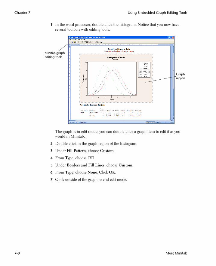
Chapter 7 Using Embedded Graph Editing Tools
7-8 Meet Minitab
1 In the word processor, double-click the histogram. Notice that you now have several toolbars with editing tools.
The graph is in edit mode; you can double-click a graph item to edit it as you would in Minitab.
2 Double-click in the graph region of the histogram.
3 Under Fill Pattern, choose Custom.
4 From Type, choose .
5 Under Borders and Fill Lines, choose Custom.
6 From Type, choose None. Click OK.
7 Click outside of the graph to end edit mode.
Minitab graph editing tools
Graph region
MeetMinitab.book Page 8 Monday, April 6, 2009 11:25 AM

Sending Output to Microsoft PowerPoint Generating a Report
Meet Minitab 7-9
Save project Save all of your work in a Minitab project.
1 In Minitab, Choose File ➤ Save Project As.
2 In File name, type My_Reports.MPJ.
3 Click Save.
Sending Output to Microsoft PowerPointYou can also create reports or presentations by sending graphs and Session window output directly to Microsoft Word or PowerPoint.
Add the histogram and descriptive statistics results to PowerPoint.
For more information about Minitab’s Embedded Graph Editor, go to Embedded graph editor in the Minitab Help index.
MeetMinitab.book Page 9 Monday, April 6, 2009 11:25 AM

Chapter 7 Sending Output to Microsoft PowerPoint
7-10 Meet Minitab
Sendoutput to
PowerPoint
1 Choose Window ➤ Histogram of Days.
2 Right-click anywhere in the graph region, then choose Send Graph to Microsoft PowerPoint. A new PowerPoint file will open with the histogram on the first slide.
3 In Minitab, choose Window ➤ Session.
4 In the Session window, click in the output for Results for Center = Central. Then right-click and choose Send Section to Microsoft PowerPoint.
5 Repeat step 4 for Results for Center = Eastern and Results for Center = Western.
MeetMinitab.book Page 10 Monday, April 6, 2009 11:25 AM

What’s Next Generating a Report
Meet Minitab 7-11
A new Microsoft PowerPoint document contains the histogram and each part of the Session window output on separate slides. You can edit the PowerPoint document to changes titles or font sizes and add text.
What’s NextIn the next chapter, you learn to prepare a Minitab worksheet. You combine data from multiple sources and place them in Minitab. Also, to prepare the data and simplify the analysis, you edit the data and reorganize columns and rows.
To add multiple sections of Session window output to the Word or PowerPoint:1 Highlight the Session window output.2 Right-click in the Session window.3 Choose Send Selected Lines to Microsoft Word or Send Selected Lines to Microsoft
PowerPoint.
When you send a graph to Word or PowerPoint, Minitab’s Embedded Graph Editor is not available.
MeetMinitab.book Page 11 Monday, April 6, 2009 11:25 AM

Chapter 7 What’s Next
7-12 Meet Minitab
MeetMinitab.book Page 12 Monday, April 6, 2009 11:25 AM

Meet Minitab 8-1
8Preparing a Worksheet
ObjectivesIn this chapter, you:
■ Open a worksheet, page 8-2
■ Merge data from an Excel spreadsheet into a Minitab worksheet, page 8-3
■ Merge data from a text file into a worksheet, page 8-4
■ View worksheet information, page 8-5
■ Replace missing value, page 8-6
■ Stack columns of data, page 8-6
■ Code data, page 8-8
■ Add column names, page 8-8
■ Insert and name a new data column, page 8-9
■ Use the Calculator to assign a formula to a column, page 8-9
OverviewIn many cases, you use worksheets that were already set up for you, as you have throughout Meet Minitab. Sometimes, however, you must combine data from different sources and place them in a Minitab worksheet before beginning an analysis. Minitab can use data from:
■ Previously saved Minitab worksheet files
■ Text files
MeetMinitab.book Page 1 Monday, April 6, 2009 11:25 AM
Chapter 8 Getting Data from Different Sources
8-2 Meet Minitab
■ Microsoft Excel documents
To place these data in Minitab, you can:
■ Type directly into Minitab
■ Copy and paste from other applications
■ Open from a variety of file types, including Excel or text files
After your data are in Minitab, you may need to edit cells and reorganize columns and rows to get the data ready for analysis. Common manipulations include stacking, subsetting, specifying column names, and editing data values.
This chapter shows how to place data from different sources into Minitab and how ShippingData.MTW, used in chapters 2 and 3, was prepared for analysis.
Getting Data from Different SourcesFor the initial Meet Minitab analyses, the worksheet ShippingData.MTW, which contains data from three shipping centers, was already set up. However, the three shipping centers originally stored the book order data in different ways:
■ Eastern—in a Minitab worksheet
■ Central—in a Microsoft Excel file
■ Western—in a text file
To analyze all the book order data, you must combine the data from all three shipping centers into a single Minitab worksheet.
Open aworksheet
Begin with data from the Eastern shipping center, which are stored in a Minitab worksheet called Eastern.MTW.
1 If continuing from the previous chapter, choose File ➤ New, then choose Minitab Project and click OK. Otherwise, just start Minitab.
2 Choose File ➤ Open Worksheet.
3 Click Look in Minitab Sample Data folder, near the bottom of the dialog box.
4 In the Sample Data folder, double-click Meet Minitab, then choose Eastern.MTW. Click Open.
Minitab can open a variety of file types. To see the file types, click Files of type in the Open Worksheet dialog box.
MeetMinitab.book Page 2 Monday, April 6, 2009 11:25 AM
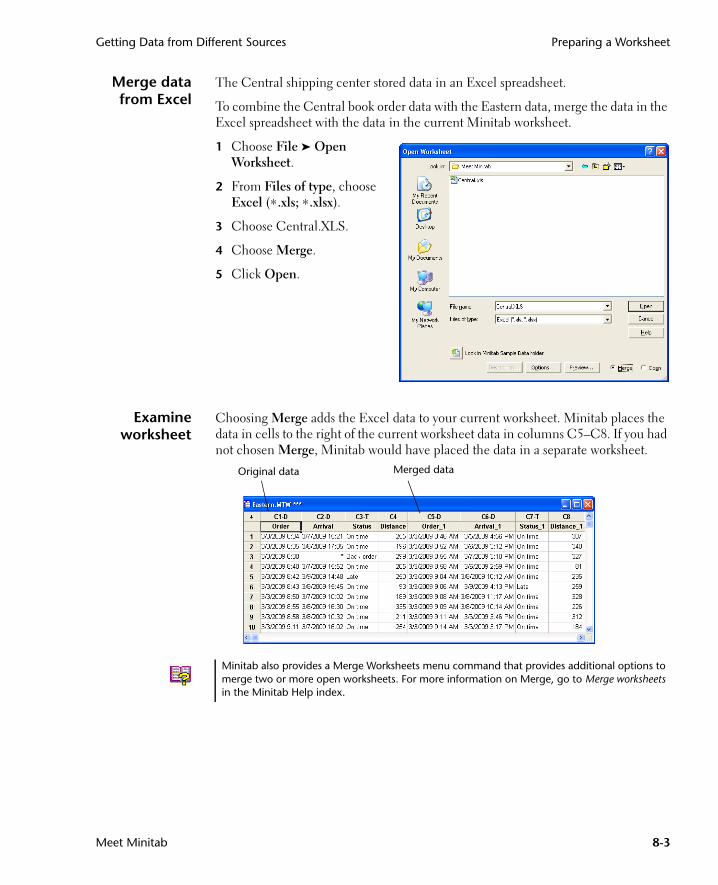
Getting Data from Different Sources Preparing a Worksheet
Meet Minitab 8-3
Merge datafrom Excel
The Central shipping center stored data in an Excel spreadsheet.
To combine the Central book order data with the Eastern data, merge the data in the Excel spreadsheet with the data in the current Minitab worksheet.
1 Choose File ➤ Open Worksheet.
2 From Files of type, choose Excel (∗.xls; ∗.xlsx).
3 Choose Central.XLS.
4 Choose Merge.
5 Click Open.
Examineworksheet
Choosing Merge adds the Excel data to your current worksheet. Minitab places the data in cells to the right of the current worksheet data in columns C5–C8. If you had not chosen Merge, Minitab would have placed the data in a separate worksheet.
Original data Merged data
Minitab also provides a Merge Worksheets menu command that provides additional options to merge two or more open worksheets. For more information on Merge, go to Merge worksheets in the Minitab Help index.
MeetMinitab.book Page 3 Monday, April 6, 2009 11:25 AM

Chapter 8 Preparing the Worksheet for Analysis
8-4 Meet Minitab
Merge datafrom a text
file
The Western shipping center stored data in a simple text file that you can open using Notepad or WordPad. To combine the Western book order data with the Eastern and Central data, merge the data in the text file with the data in the current Minitab worksheet.
1 Choose File ➤ Open Worksheet
2 From Files of type, choose Text (∗.txt).
3 Choose Western.TXT.
4 Choose Merge.
5 Click Open.
Examineworksheet
Choosing Merge adds the data from the text file to the current worksheet. Minitab places the data in cells to the right of the current worksheet data in columns C9–C12. If you had not chosen Merge, Minitab would have placed the data in a separate worksheet,
Before opening a text file in Minitab, you can see what the data will look like in the worksheet by choosing Preview in the Open Worksheet dialog box.
Preparing the Worksheet for AnalysisWith the data in a single worksheet, you are almost ready to begin the analysis. However, you must modify the worksheet by:
■ Replacing a missing value
■ Stacking data
■ Replacing data
Original data Merged data
Not all text files are in a format that can be easily imported. Minitab provides several tools for interpreting text file formats. For more information, go to Text files in the Minitab Help index.
MeetMinitab.book Page 4 Monday, April 6, 2009 11:25 AM

Preparing the Worksheet for Analysis Preparing a Worksheet
Meet Minitab 8-5
■ Adding column names
■ Adding a new column
■ Creating a column of calculated values
Showworksheet
information
To view a summary of your worksheet columns, use on the Project Manager toolbar. This button will open the Project Manager’s Columns subfolder in the Worksheets folder. This summary is especially useful in identifying unequal column lengths or columns that contain missing values.
1 Click on the Project Manager toolbar or press [Ctrl]+[Alt]+[I].
The Columns subfolder contains details on the current worksheet. Within each center, the count should be the same for all columns. Notice that the counts for the Eastern data (C1–C4) are 109 for all columns, and the counts for the Central data (C5–C8) are 105 for all columns. However, for the Western center, C10 has a count of 104 unlike the other columns, which have a count of 105.
2 Click again to return to your previous view.
For a complete list of data manipulations available in Minitab, go to Data menu in the Minitab Help index.
For more information on the Project Manager toolbar, go to Project Manager Toolbar in the Minitab Help index.
MeetMinitab.book Page 5 Monday, April 6, 2009 11:25 AM

Chapter 8 Preparing the Worksheet for Analysis
8-6 Meet Minitab
Examineworksheet
Examine C10 to see what value is missing. Notice that the last row of the column is empty. When you copy and paste data from a text or Excel file into a worksheet, Minitab interprets empty numeric or data/time cells as missing values, which appear as asterisks (∗) by default. However, if the last row of a column of data in a text file contains an empty cell, Minitab leaves the cell empty when you paste the data into the worksheet, as you can see in column C10.
Replacemissing value
For Minitab to perform the correct analysis, you must type the missing value symbol in the empty cell of the last row.
1 Click the Data window to make it active, then choose Editor ➤ Go To….
2 In Enter column number or name, type C10.
3 In Enter row number, type 105. Click OK.
4 In row 105 of column C10, type an asterisk (∗). Press [Enter].
Stack data Now that the data are assembled in a single Minitab worksheet, notice the similar variables for each shipping center. Some Minitab commands allow data from different groups to remain unstacked in separate columns. Others require groups to be stacked, with a column of group levels. However, all analyses can be performed with stacked data.
To analyze the data, you need to rearrange these variables into stacked columns. You can move data within the worksheet by copying and pasting or use Data menu items to rearrange blocks of data.
Empty cell
MeetMinitab.book Page 6 Monday, April 6, 2009 11:25 AM

Preparing the Worksheet for Analysis Preparing a Worksheet
Meet Minitab 8-7
1 Choose Data ➤ Stack ➤ Blocks of Columns.
2 From the list of variables, highlight Order, Arrival, Status, and Distance. Click Select to move the variables into the first row of Stack two or more blocks of columns on top of each other. Move to the next row.
3 Repeat step 2 for the order, arrival, status, and distance columns for the Central and Western shipping centers.
4 Under Store stacked data in, choose New worksheet. In Name, type My_ShippingData.
5 Check Use variable names in subscript column.
6 Click OK.
Examineworksheet
The variables for the shipping centers are all in the same columns, with Order (Eastern center), Order_1 (Central center), and Order_2 (Western center) acting as labels or subscripts to indicate from which shipping center the data originated.
Subscripts column
Data entry arrow
MeetMinitab.book Page 7 Monday, April 6, 2009 11:25 AM
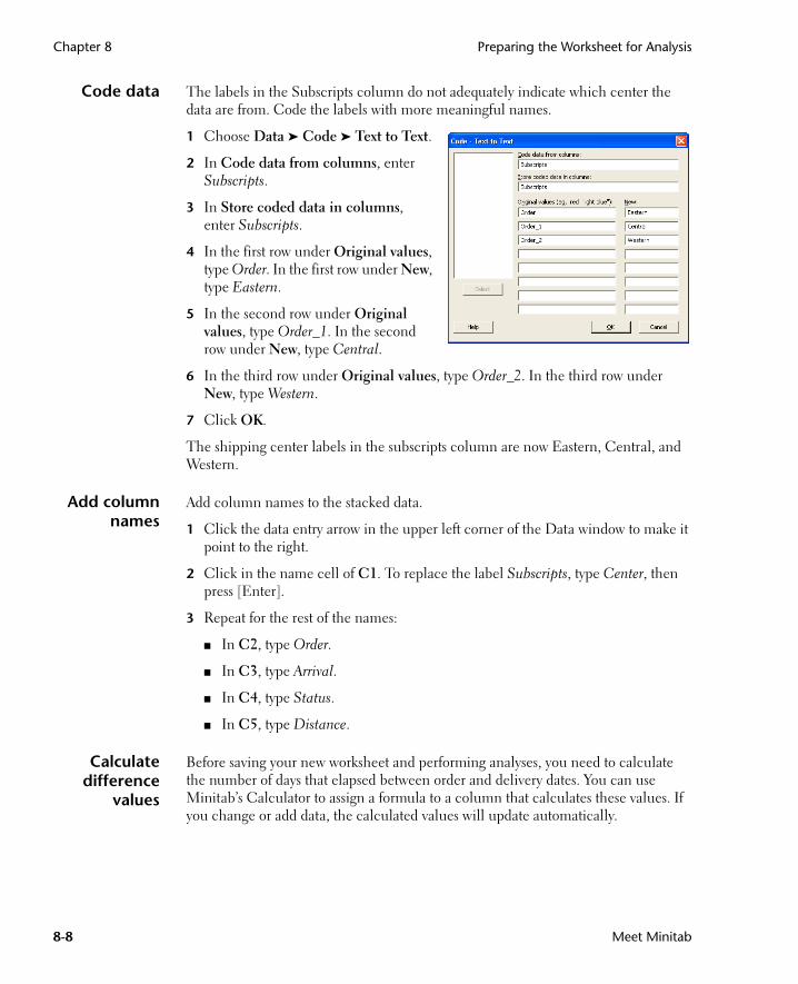
Chapter 8 Preparing the Worksheet for Analysis
8-8 Meet Minitab
Code data The labels in the Subscripts column do not adequately indicate which center the data are from. Code the labels with more meaningful names.
1 Choose Data ➤ Code ➤ Text to Text.
2 In Code data from columns, enter Subscripts.
3 In Store coded data in columns, enter Subscripts.
4 In the first row under Original values, type Order. In the first row under New, type Eastern.
5 In the second row under Original values, type Order_1. In the second row under New, type Central.
6 In the third row under Original values, type Order_2. In the third row under New, type Western.
7 Click OK.
The shipping center labels in the subscripts column are now Eastern, Central, and Western.
Add columnnames
Add column names to the stacked data.
1 Click the data entry arrow in the upper left corner of the Data window to make it point to the right.
2 Click in the name cell of C1. To replace the label Subscripts, type Center, then press [Enter].
3 Repeat for the rest of the names:
■ In C2, type Order.
■ In C3, type Arrival.
■ In C4, type Status.
■ In C5, type Distance.
Calculatedifference
values
Before saving your new worksheet and performing analyses, you need to calculate the number of days that elapsed between order and delivery dates. You can use Minitab’s Calculator to assign a formula to a column that calculates these values. If you change or add data, the calculated values will update automatically.
MeetMinitab.book Page 8 Monday, April 6, 2009 11:25 AM
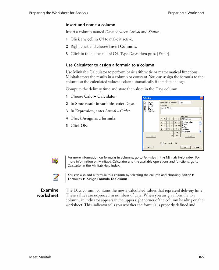
Preparing the Worksheet for Analysis Preparing a Worksheet
Meet Minitab 8-9
Insert and name a column
Insert a column named Days between Arrival and Status.
1 Click any cell in C4 to make it active.
2 Right-click and choose Insert Columns.
3 Click in the name cell of C4. Type Days, then press [Enter].
Use Calculator to assign a formula to a column
Use Minitab’s Calculator to perform basic arithmetic or mathematical functions. Minitab stores the results in a column or constant. You can assign the formula to the column so the calculated values update automatically if the data change.
Compute the delivery time and store the values in the Days column.
1 Choose Calc ➤ Calculator.
2 In Store result in variable, enter Days.
3 In Expression, enter Arrival – Order.
4 Check Assign as a formula.
5 Click OK.
Examineworksheet
The Days column contains the newly calculated values that represent delivery time. These values are expressed in numbers of days. When you assign a formula to a column, an indicator appears in the upper right corner of the column heading on the worksheet. This indicator tells you whether the formula is properly defined and
For more information on formulas in columns, go to Formulas in the Minitab Help index. For more information on Minitab’s Calculator and the available operations and functions, go to Calculator in the Minitab Help index.
You can also add a formula to a column by selecting the column and choosing Editor ➤ Formulas ➤ Assign Formula To Column.
MeetMinitab.book Page 9 Monday, April 6, 2009 11:25 AM

Chapter 8 Preparing the Worksheet for Analysis
8-10 Meet Minitab
whether the data need to be updated by re-calculating the values. The green plus sign indicates the data are up-to-date.
Updateworksheet
Suppose you learn that the arrival date for a shipment in the Central shipping center is incorrect. You can correct the date in the worksheet and Minitab will automatically update the Days column.
Update the arrival date in row 127 from 3/6/2009 to 3/7/2009.
1 In row 127 of the worksheet, edit the day in the date in the Arrival column by double-clicking the cell to put it in edit mode. Change 3/6/2009 to 3/7/2009.
2 Press [Enter].
Examineworksheet
Minitab automatically updates the value in the Days column from 2.98125 to 3.98125.
Status indicator
Place your cursor over the status indicator to view the formula assigned to the column. Double-click the status indicator to edit the formula.
Original worksheet Updated worksheet
You can also choose to update the calculated values manually. First, choose Editor ➤ Formulas ➤ Calculate All Formulas Automatically to uncheck this option. When the status indicator is yellow, indicating formulas are out of date, you can choose Editor ➤ Formulas ➤ Calculate All Formulas Now to update all formulas in the project. This command is active only if formulas are out of date and Calculate All Formulas Automatically is not checked in the Editor menu.
MeetMinitab.book Page 10 Monday, April 6, 2009 11:25 AM
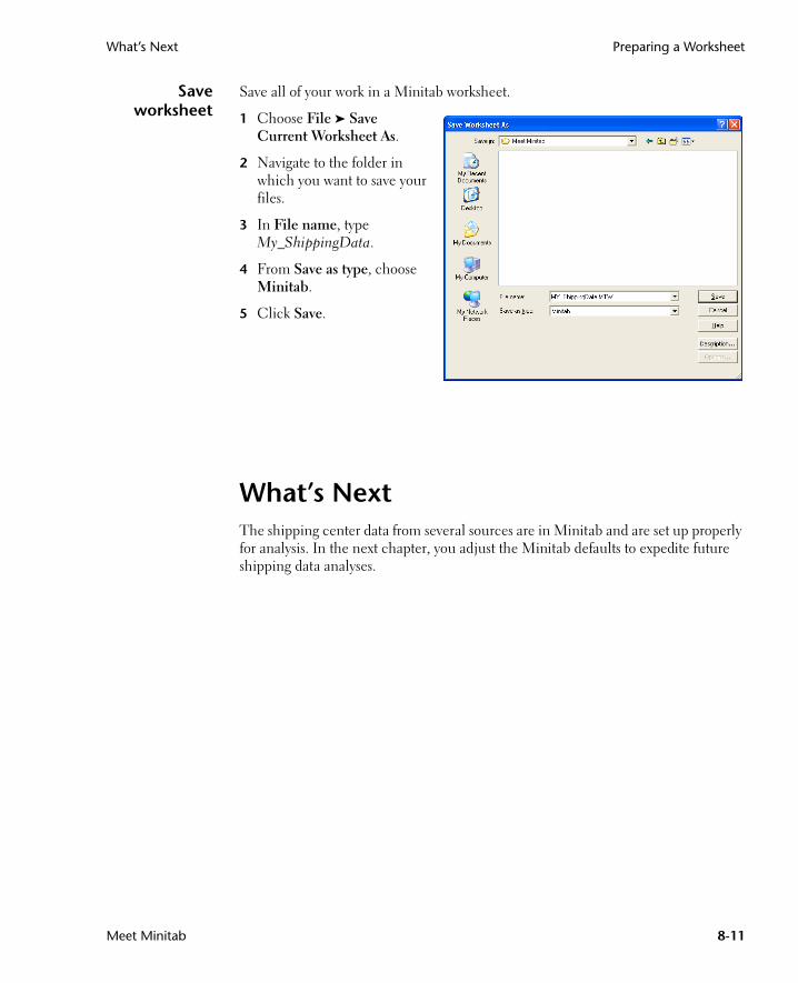
What’s Next Preparing a Worksheet
Meet Minitab 8-11
Saveworksheet
Save all of your work in a Minitab worksheet.
1 Choose File ➤ Save Current Worksheet As.
2 Navigate to the folder in which you want to save your files.
3 In File name, type My_ShippingData.
4 From Save as type, choose Minitab.
5 Click Save.
What’s NextThe shipping center data from several sources are in Minitab and are set up properly for analysis. In the next chapter, you adjust the Minitab defaults to expedite future shipping data analyses.
MeetMinitab.book Page 11 Monday, April 6, 2009 11:25 AM

Chapter 8 What’s Next
8-12 Meet Minitab
MeetMinitab.book Page 12 Monday, April 6, 2009 11:25 AM
Meet Minitab 9-1
9Customizing Minitab
ObjectivesIn this chapter, you:
■ Change default options for graphs, page 9-2
■ Create a new toolbar, page 9-3
■ Add commands to a custom toolbar, page 9-4
■ Assign shortcut keys for a menu command, page 9-5
■ Restore your Minitab default settings using Manage Profiles, page 9-7
OverviewMinitab has several tools for changing default options or creating custom tools such as individualized toolbars or keyboard shortcuts.
Use Tools ➤ Options to change defaults for:
■ Program settings (memory usage, initial directory, window layout, and dialog box)
■ Data and Session windows
■ Statistical commands
■ Graphs
Use Tools ➤ Customize to:
■ Assign a shortcut key to a menu item
■ Set options for how Minitab displays toolbars
■ Create custom icons for menu items or toolbar buttons
Now that you have completed your first book shipment analysis and generated a report, you decide to use Tools ➤ Options and Tools ➤ Customize to tailor the Minitab environment to make future analyses quicker and easier.
MeetMinitab.book Page 1 Monday, April 6, 2009 11:25 AM

Chapter 9 Setting Options
9-2 Meet Minitab
Setting OptionsYou can change many options during a Minitab session, such as changing graph display settings or enabling the session command prompt. However, when you exit Minitab, these options revert back to the defaults for future Minitab sessions.
If you want a setting to be your default for all Minitab sessions, use Tools ➤ Options. Settings that you change remain active until you change them again.
Because you are planning to do similar analyses on the shipping data during the next few months, you want to change your default preferences.
Addautomatic
footnote
Because you will create the same graphs with similar data in the future, you need a way to distinguish the results of each analysis. You decide to add an automatic footnote to your graphs to include the worksheet name, last modification date, and some information on the data used.
1 If continuing from the previous chapter, choose File ➤ New, then choose Minitab Project and click OK. Otherwise, just start Minitab.
2 Choose File ➤ Open Worksheet.
3 Click Look in Minitab Sample Data folder, near the bottom of the dialog box.
4 In the Sample Data folder, double-click Meet Minitab, then choose ShippingData.MTW. Click Open.
5 Choose Tools ➤ Options ➤ Graphics ➤ Annotation ➤ My Footnote.
6 Under Information to include in my footnote, check Worksheet name and Date the graph was last modified.
7 In Custom text, type Shipping center efficiency. Click OK.
With these settings, every time you create a graph, Minitab adds the automatic footnote.
If you change options, you can restore Minitab’s default settings at any time. For more information, see Restoring Minitab’s Default Settings on page 9-6.
MeetMinitab.book Page 2 Monday, April 6, 2009 11:25 AM

Creating a Custom Toolbar Customizing Minitab
Meet Minitab 9-3
Create ahistogram to
view footnote
To see an example of the automatic footnote, create a histogram.
1 Choose Graph ➤ Histogram.
2 Choose With Fit and Groups, then click OK.
3 In Graph variables, enter Days.
4 In Categorical variables for grouping (0-3), enter Center.
5 Click OK.
Creating a Custom ToolbarIn addition to saving time by changing the default options settings for individual commands, you also can save time in future Minitab sessions by using Tools ➤ Customize.
Use Customize to create new menus and toolbars that contain only the commands you choose to add, and to assign keyboard shortcuts to commands that you access frequently.
Create atoolbar
During some analyses, you return to the same menu items many times. Combining these items on a single custom toolbar can simplify future analysis.
Create a custom toolbar that includes some of the commands used in the shipping center analysis.
Automatic footnote
MeetMinitab.book Page 3 Monday, April 6, 2009 11:25 AM
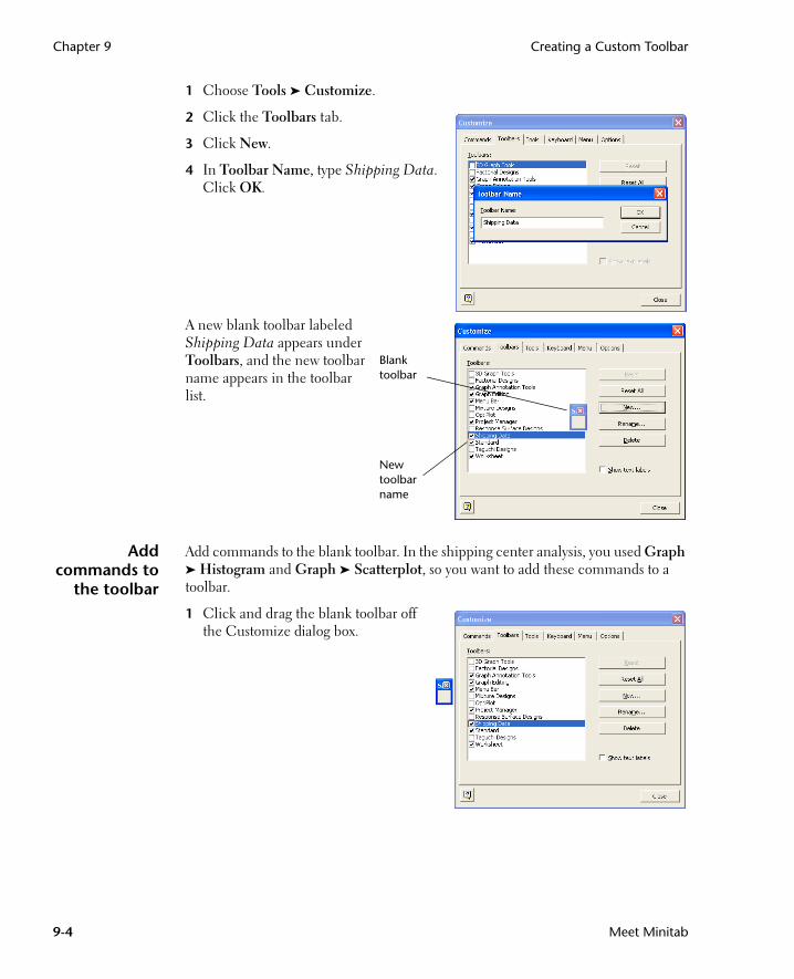
Chapter 9 Creating a Custom Toolbar
9-4 Meet Minitab
1 Choose Tools ➤ Customize.
2 Click the Toolbars tab.
3 Click New.
4 In Toolbar Name, type Shipping Data. Click OK.
A new blank toolbar labeled Shipping Data appears under Toolbars, and the new toolbar name appears in the toolbar list.
Addcommands to
the toolbar
Add commands to the blank toolbar. In the shipping center analysis, you used Graph ➤ Histogram and Graph ➤ Scatterplot, so you want to add these commands to a toolbar.
1 Click and drag the blank toolbar off the Customize dialog box.
Blank toolbar
New toolbar name
MeetMinitab.book Page 4 Monday, April 6, 2009 11:25 AM
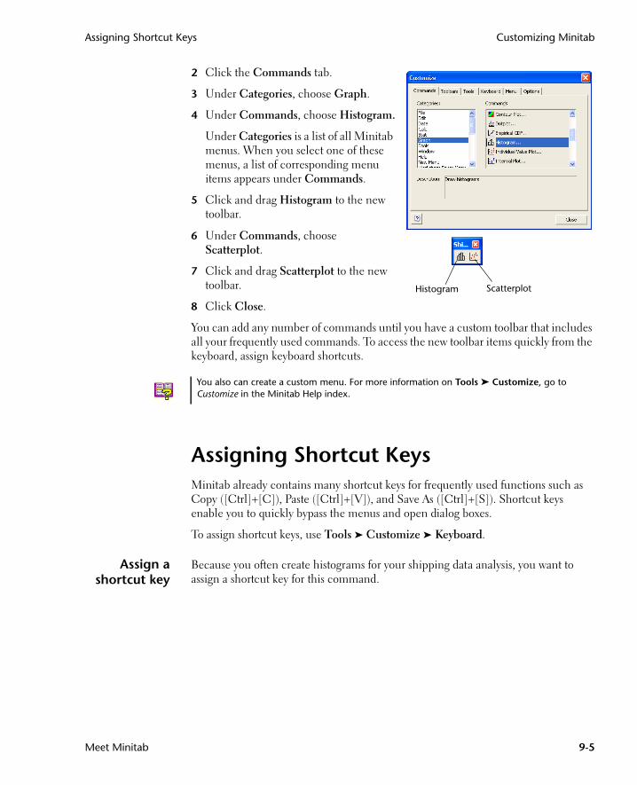
Assigning Shortcut Keys Customizing Minitab
Meet Minitab 9-5
2 Click the Commands tab.
3 Under Categories, choose Graph.
4 Under Commands, choose Histogram.
Under Categories is a list of all Minitab menus. When you select one of these menus, a list of corresponding menu items appears under Commands.
5 Click and drag Histogram to the new toolbar.
6 Under Commands, choose Scatterplot.
7 Click and drag Scatterplot to the new toolbar.
8 Click Close.
You can add any number of commands until you have a custom toolbar that includes all your frequently used commands. To access the new toolbar items quickly from the keyboard, assign keyboard shortcuts.
Assigning Shortcut KeysMinitab already contains many shortcut keys for frequently used functions such as Copy ([Ctrl]+[C]), Paste ([Ctrl]+[V]), and Save As ([Ctrl]+[S]). Shortcut keys enable you to quickly bypass the menus and open dialog boxes.
To assign shortcut keys, use Tools ➤ Customize ➤ Keyboard.
Assign ashortcut key
Because you often create histograms for your shipping data analysis, you want to assign a shortcut key for this command.
Histogram Scatterplot
You also can create a custom menu. For more information on Tools ➤ Customize, go to Customize in the Minitab Help index.
MeetMinitab.book Page 5 Monday, April 6, 2009 11:25 AM
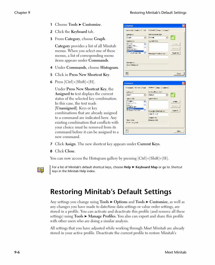
Chapter 9 Restoring Minitab’s Default Settings
9-6 Meet Minitab
1 Choose Tools ➤ Customize.
2 Click the Keyboard tab.
3 From Category, choose Graph.
Category provides a list of all Minitab menus. When you select one of these menus, a list of corresponding menu items appears under Commands.
4 Under Commands, choose Histogram.
5 Click in Press New Shortcut Key.
6 Press [Ctrl]+[Shift]+[H].
Under Press New Shortcut Key, the Assigned to text displays the current status of the selected key combination. In this case, the text reads [Unassigned]. Keys or key combinations that are already assigned to a command are indicated here. Any existing combination that conflicts with your choice must be removed from its command before it can be assigned to a new command.
7 Click Assign. The new shortcut key appears under Current Keys.
8 Click Close.
You can now access the Histogram gallery by pressing [Ctrl]+[Shift]+[H].
Restoring Minitab’s Default SettingsAny settings you change using Tools ➤ Options and Tools ➤ Customize, as well as any changes you have made to date/time data settings or value order settings, are stored in a profile. You can activate and deactivate this profile (and remove all these settings) using Tools ➤ Manage Profiles. You also can export and share this profile with other users who are doing a similar analysis.
All settings that you have adjusted while working through Meet Minitab are already stored in your active profile. Deactivate the current profile to restore Minitab’s
For a list of Minitab’s default shortcut keys, choose Help ➤ Keyboard Map or go to Shortcut keys in the Minitab Help index.
MeetMinitab.book Page 6 Monday, April 6, 2009 11:25 AM

What’s Next Customizing Minitab
Meet Minitab 9-7
default settings and change the name of the profile to use for future shipping center analyses.
Restoredefaults
1 Choose Tools ➤ Manage Profiles.
2 Click to move MyProfile from Active profiles to Available profiles.
3 Double-click MyProfile in Available profiles, then type ShippingCenterAnalysis.
4 Click OK.
The default settings are now restored. Minitab creates a new active profile to store any changes you make after this point.
To activate the settings you adjusted during your Meet Minitab sessions, move the current active profile to Available profiles, move ShippingCenterAnalysis to Active profiles, then click OK.
Save project Save all of your work in a Minitab project.
1 Choose File ➤ Save Project As.
2 Navigate to the folder in which you want to save your files.
3 In File name, type My_Customize.MPJ.
4 Click Save.
What’s NextYour analysis is complete, but what do you do if you have questions or want more information about a topic? The next chapter suggests ways to get answers to your Minitab questions and provides details about how to use Minitab Help and StatGuide.
For more information on managing profiles, go to Manage Profiles in the Minitab Help index.
You also can reset Minitab’s defaults by double-clicking the shortcut named Restore Minitab Defaults English located in the English folder under the main Minitab 16 folder installed on your hard drive. Export any profiles you want to keep before running this program.
MeetMinitab.book Page 7 Monday, April 6, 2009 11:25 AM

Chapter 9 What’s Next
9-8 Meet Minitab
MeetMinitab.book Page 8 Monday, April 6, 2009 11:25 AM
Meet Minitab 10-1
10Getting Help
ObjectivesIn this chapter, you:
■ Get answers and find information, page 10-2
■ Use Minitab Help, page 10-6
■ Use Minitab StatGuide, page 10-8
■ Use Session Command Help, page 10-10
OverviewIf you find yourself with unanswered questions or discover that you need more details about a topic, Minitab can help.
From assistance with completing a dialog box, to guidance for statistical interpretations, to instructions for using session commands in your analysis, Minitab’s easy-to-use online documentation and Internet resources can help you find the answers you need.
This chapter discusses using Help, StatGuide, and Session Command Help to explore Minitab and suggests ways to find answers to your Minitab questions.
MeetMinitab.book Page 1 Monday, April 6, 2009 11:25 AM

Chapter 10 Getting Answers and Information
10-2 Meet Minitab
Getting Answers and InformationMeet Minitab focused on only a few of Minitab’s commonly used features. For details about other commands, functions, and statistical concepts, explore Minitab’s documentation and online resources.
Resource Description Access
Help Documentation on Minitab features and concepts. Includes information on:
■ Menus and dialog boxes
■ Methods and formulas
■ Session commands
■ Macros
■ Click Help in any dialog box.
■ Click on the toolbar.
■ Press [F1] at any time.
■ Choose Help ➤ Help.
See Help on page 10-6 for more information.
Using Help
General information on navigating Minitab Help.
Choose Help ➤ Help, then click Using Help under Basics.
StatGuide Statistical guidance that focuses on interpretation of sample results.
■ Right-click in the Session window or a Graph window, then choose StatGuide.
■ Right-click in the Session or Graph folder of the Project Manager, then choose StatGuide.
■ Click on the toolbar.
■ Press [Shift]+[F1].
■ Choose Help ➤ StatGuide.
See StatGuide on page 10-8 for more information.
Minitab Statistical Glossary
This comprehensive glossary covers all areas of Minitab statistics. Each definition contains practical, easy-to-understand information.
Choose Help ➤ Glossary.
Tutorials Tutorials show you how to use different analyses in your own Minitab sessions, and include easy-to-understand data requirements and step-by-step examples.
Choose Help ➤ Tutorials.
MeetMinitab.book Page 2 Monday, April 6, 2009 11:25 AM
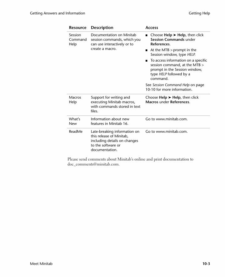
Getting Answers and Information Getting Help
Meet Minitab 10-3
Please send comments about Minitab’s online and print documentation to [email protected].
Session Command Help
Documentation on Minitab session commands, which you can use interactively or to create a macro.
■ Choose Help ➤ Help, then click Session Commands under References.
■ At the MTB > prompt in the Session window, type HELP.
■ To access information on a specific session command, at the MTB > prompt in the Session window, type HELP followed by a command.
See Session Command Help on page 10-10 for more information.
Macros Help
Support for writing and executing Minitab macros, with commands stored in text files.
Choose Help ➤ Help, then click Macros under References.
What’s New
Information about new features in Minitab 16.
Go to www.minitab.com.
ReadMe Late-breaking information on this release of Minitab, including details on changes to the software or documentation.
Go to www.minitab.com.
Resource Description Access
MeetMinitab.book Page 3 Monday, April 6, 2009 11:25 AM
Chapter 10 Minitab Help Overview
10-4 Meet Minitab
Minitab Help OverviewThe components of Minitab’s online documentation—as well as other related information—are summarized on a single page. From this page, you can proceed to detailed assistance, instructions, and support topics. This overview organizes links to Help topics according to Minitab’s menu structure.
Findinginformation
To display the overview page:
■ Choose Help ➤ Help.
■ Press [F1].
■ Click on the Standard toolbar.
The links provided under the headings shown below make finding information quick and easy:
■ Basics—how to use Help, guidelines and tutorials for getting started with Minitab, and descriptions of Minitab windows
■ References—examples of commands, glossary of terms and abbreviations, instructions for using session commands and macros, and the methods and formulas used by Minitab
■ Service and Support—how to register Minitab, ways to communicate with Technical Support, and descriptions of Minitab’s documentation, Internet resources, and other products
MeetMinitab.book Page 4 Monday, April 6, 2009 11:25 AM

Minitab Help Overview Getting Help
Meet Minitab 10-5
For more information about the Minitab Help environment, choose Help ➤ Help, then click Using Help under Basics.
Use these links to access basic facts, reference material, and service and support information.
Click a menu link to view Help topics for all commands on that menu.
MeetMinitab.book Page 5 Monday, April 6, 2009 11:25 AM

Chapter 10 Help
10-6 Meet Minitab
HelpMinitab Help is a comprehensive, convenient source of information that includes menu and dialog box instructions, overviews, examples, guidance for setting up your data, and methods and formulas. You can explore Minitab’s statistical features and discover new methods for routine tasks. Help also provides guidance on using Minitab’s statistics, quality control, reliability and survival analysis, and design of experiments tools.
Additionally, in Help, you can learn about the Minitab environment; using session commands; writing macros and Execs; Minitab’s input, output, and data manipulation capabilities; and working with data and graphs.
Findinginformation
Most Help topics appear in a window that consists of three areas:
■ Toolbar—contains buttons for hiding and showing the navigation pane, returning to a previous topic, printing one or more topics, and tools for working within the Help environment
■ Navigation pane—provides three tabs for exploring the table of contents and index, and searching for words or phrases
■ Topic pane—displays the selected Help topic
Toolbar
Navigation pane
■ Contents—Click any folder or topic for more information.
■ Index—Search the index for a term, or scroll through the list.
■ Search—Search the Help for specific words or phrases.
Topic pane
MeetMinitab.book Page 6 Monday, April 6, 2009 11:25 AM
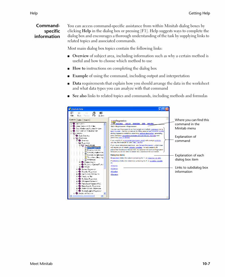
Help Getting Help
Meet Minitab 10-7
Command-specific
information
You can access command-specific assistance from within Minitab dialog boxes by clicking Help in the dialog box or pressing [F1]. Help suggests ways to complete the dialog box and encourages a thorough understanding of the task by supplying links to related topics and associated commands.
Most main dialog box topics contain the following links:
■ Overview of subject area, including information such as why a certain method is useful and how to choose which method to use
■ How to instructions on completing the dialog box
■ Example of using the command, including output and interpretation
■ Data requirements that explain how you should arrange the data in the worksheet and what data types you can analyze with that command
■ See also links to related topics and commands, including methods and formulas
Links to subdialog box information
Where you can find this command in the Minitab menu
Explanation of each dialog box item
Explanation of command
MeetMinitab.book Page 7 Monday, April 6, 2009 11:25 AM
Chapter 10 StatGuide
10-8 Meet Minitab
StatGuideThe Minitab StatGuide explains how to interpret statistical tables and graphs in a practical, easy-to-understand way. Unlike Help, which provides guidance for using Minitab, the StatGuide focuses on the interpretation of Minitab results, using preselected examples to explain the output.
StatGuide topics include information such as:
■ Real-life data analysis situations
■ Brief summaries of statistical capabilities
■ Emphasis on important components of the output
Findinginformation
After you issue a command, you can learn more about the output by examining StatGuide’s example output and interpretation. The StatGuide provides a direct path to command-specific guidance:
■ Right-click in the Session window output or on a graph, then choose StatGuide.
■ Click in the Session window output or on a graph, then click on the toolbar or press [Shift]+[F1].
■ In the Project Manager, click the name of the Session window output or graph, then click on the toolbar or press [Shift]+[F1]. You can also right-click the Session window or graph output name, then choose StatGuide.
You can also access the StatGuide by choosing Help ➤ StatGuide. To locate specific words or phrases, choose Help ➤ StatGuide, then click the Search tab.
MeetMinitab.book Page 8 Monday, April 6, 2009 11:25 AM

StatGuide Getting Help
Meet Minitab 10-9
Command-specific
information
Each topic in the StatGuide provides interpretation for a part of the Session window output or graph and includes the following sections:
■ The first section directly below the main heading contains general guidance on interpreting the output or graph.
■ The Example Output section contains the output or graph.
■ The Interpretation section contains specific interpretation for the output or graph shown in the topic.
Browse all StatGuide topics for a command.
Display a list of all StatGuide topics for a command.
View in-depth content for more information about the analysis.
Read a description of the data used in the example output.
Lists available topics for each command and shows your location within the StatGuide.
MeetMinitab.book Page 9 Monday, April 6, 2009 11:25 AM

Chapter 10 Session Command Help
10-10 Meet Minitab
Session Command Help In addition to using Minitab’s menus and dialog boxes, you can also conduct analyses, generate graphs, and manipulate data using session commands. Each Minitab menu command has a corresponding session command, which consists of a main command and, usually, one or more subcommands. Session commands are especially useful because they can be used to create macros, which are session commands stored in a text file. Macros can help automate repeated tasks. See Help ➤ Help, then click Macros under References for more information about how to write Execs and macros.
Findinginformation
To access Minitab Session Command Help, choose Help ➤ Help, then click Session Commands under References.
The Session Command Help environment is similar to Minitab Help. The toolbar, navigation pane, and topic pane provide the necessary tools for learning and using session commands.
View these topics for instructions on how to use session commands and macros.
View these topics for lists of commands and macros.
To learn more about session commands, go to Chapter 6, Using Session Commands.
MeetMinitab.book Page 10 Monday, April 6, 2009 11:25 AM
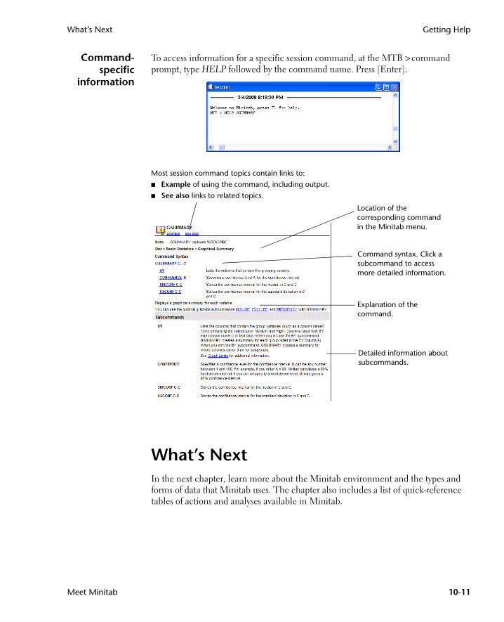
What’s Next Getting Help
Meet Minitab 10-11
Command-specific
information
To access information for a specific session command, at the MTB > command prompt, type HELP followed by the command name. Press [Enter].
What’s NextIn the next chapter, learn more about the Minitab environment and the types and forms of data that Minitab uses. The chapter also includes a list of quick-reference tables of actions and analyses available in Minitab.
Command syntax. Click a subcommand to access more detailed information.
Location of the corresponding command in the Minitab menu.
Most session command topics contain links to:
■ Example of using the command, including output.
■ See also links to related topics.
Detailed information about subcommands.
Explanation of the command.
MeetMinitab.book Page 11 Monday, April 6, 2009 11:25 AM

Chapter 10 What’s Next
10-12 Meet Minitab
MeetMinitab.book Page 12 Monday, April 6, 2009 11:25 AM
Meet Minitab 11-1
11Reference
ObjectivesIn this chapter, you find information about:
■ Minitab environment, page 11-2
■ Minitab data, page 11-5
OverviewPrevious Meet Minitab chapters introduced you to Minitab and some of its features and commands. This chapter provides in-depth information about the Minitab environment and data, as well as quick-reference tables to help you to perform the actions and statistics you need in your own analysis.
MeetMinitab.book Page 1 Monday, April 6, 2009 11:25 AM
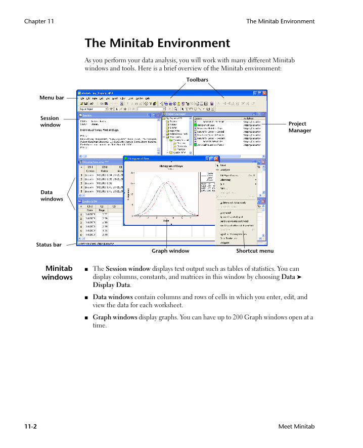
Chapter 11 The Minitab Environment
11-2 Meet Minitab
The Minitab EnvironmentAs you perform your data analysis, you will work with many different Minitab windows and tools. Here is a brief overview of the Minitab environment:
Minitabwindows
■ The Session window displays text output such as tables of statistics. You can display columns, constants, and matrices in this window by choosing Data ➤ Display Data.
■ Data windows contain columns and rows of cells in which you enter, edit, and view the data for each worksheet.
■ Graph windows display graphs. You can have up to 200 Graph windows open at a time.
Session window
Data windows
Menu bar
Shortcut menu Graph window
Project Manager
Status bar
Toolbars
MeetMinitab.book Page 2 Monday, April 6, 2009 11:25 AM

The Minitab Environment Reference
Meet Minitab 11-3
ProjectManager
The Project Manager contains folders that allow you to navigate, view, and manipulate various parts of your project. By right-clicking either the folders or the folder contents, you can access a variety of menus that allow you to manage Session window output, graphs, worksheets, command language, and related project areas.
This folder… Contains… Use to…
Session A list of:
■ All Session window output by command
■ All graphs
Manage Session window output. For example:
■ Jump to Session window output
■ Copy, delete, rename, or print Session window output or graphs
■ Append Session window output or graphs to the ReportPad
History All commands you have used
■ Repeat complex command sequences
■ Use commands to create Execs and macros
Graph A list of all graphs in your project
Manage your graphs. For example:
■ Arrange, rename, tile, or remove your graphs
■ Append graphs to the ReportPad
Folders
Contents of the open folder
MeetMinitab.book Page 3 Monday, April 6, 2009 11:25 AM

Chapter 11 The Minitab Environment
11-4 Meet Minitab
Menus andtools
Minitab provides:
■ A menu bar for choosing commands.
■ A Standard toolbar with buttons for commonly used functions−the buttons change depending on which Minitab window is active.
■ A Project Manager toolbar with shortcuts to Project Manager folders.
■ A Worksheet toolbar with buttons to insert or clear cells, rows, and columns, to move columns, and to move to the next or previous brushed row.
■ A status bar which displays explanatory text when you are pointing to a menu item or toolbar button.
■ Shortcut menus which appear when you right-click in any Minitab window or any folder in the Project Manager. The menu displays the most commonly-used functions for that window or folder.
■ Graph editing toolbars (Graph Editing, Graph Annotation Tools, and 3D Graph Tools) with buttons for adding and changing graph elements.
■ DOE toolbars (Factorial Designs, Response Surface Designs, Mixture Designs, Taguchi Designs, and OptiPlot) with buttons for DOE functions.
ReportPad A basic word processing tool
■ Create, arrange, or edit reports of project work
■ Move ReportPad contents to a more powerful word processing program for further editing and layout
Related Documents
A list of program files, documents, or Internet URLs that are related to your Minitab project
Quickly access project-related, non-Minitab files for easy reference
Worksheets The Columns, Constants, and Matrices, and Design folders for each open worksheet
View summaries of worksheet information, including:
■ Column counts, missing values, and column descriptions
■ Constants
■ Matrices
■ Design summary
This folder… Contains… Use to…
MeetMinitab.book Page 4 Monday, April 6, 2009 11:25 AM

Minitab Data Reference
Meet Minitab 11-5
■ DMAIC toolbar which organizes the statistical tools used to implement Six Sigma according to the DMAIC roadmap (Define , Measure, Analyze , Improve , and Control ).
Minitab Data
In Minitab, data are contained in a worksheet. The number of worksheets a project can have is limited only by your computer’s memory.
Data types A worksheet can contain three types of data:
■ Numeric data − Numbers.
■ Text data − Letters, numbers, spaces, and special characters. For example, Test #4 or North America.
■ Date/time data − Dates (such as Jan-1-2009, 1-Jan-2009, 3/17/09, or 17/03/09), times (such as 08:25:22 AM), or both (such as 3/17/09 08:25:22 AM or 17/03/09 08:25:22). Minitab internally stores dates and times as numbers, but displays them in the format you choose.
Forms of data Data can be in one of three forms:
The Project Manager Worksheets folder contains a list of the columns, constants, and matrices in each project.
The Graph Editing, DOE, and DMAIC toolbars are not visible at start-up, but can be opened by choosing Tools ➤ Toolbars and clicking the toolbars you want to show.
Form Contains… Referred to by... Number available
Column Numeric, text, or date/time data
■ C + number, as in C1 or C22
■ Column name, such as Center or Arrival
Limited only by computer memory, up to a maximum of 4000
Stored Constant
A single number or text string (for example, New York)
■ K + number, as in K1or K93
■ Column name, such as First or Counter
1000
Matrix A rectangular block of cells containing numbers
■ M + number, as in M1 or M44
■ Column name, such as Inverse
100
MeetMinitab.book Page 5 Monday, April 6, 2009 11:25 AM

Chapter 11 Minitab Data
11-6 Meet Minitab
Sampledata sets
Minitab comes with a number of sample data sets. The data sets used in Meet Minitab are located in the Meet Minitab folder. You can easily access the sample data sets by clicking Look in Minitab Sample Data folder near the bottom of the Open Worksheet dialog box. For complete descriptions of most of these data sets, go to Sample data sets in the Minitab Help index.
MeetMinitab.book Page 6 Monday, April 6, 2009 11:25 AM
Meet Minitab I-1
Index
Numerics3D Graph Tools toolbar 11-4
Aadding data to a worksheet 4-5analysis of variance 3-4
Tukey’s multiple comparison test 3-4
analyzing data 3-1annotating graph layout 2-13annotation, automatic 9-2ANOVA
see analysis of varianceAppend to Report 7-2arithmetic functions
see Calculatorarrow, data entry 4-5assessing quality 4-1assign formulas to a column 8-9Autofill 4-5automatic footnote, creating 9-2automating an analysis 6-7
Bboxplots of data 3-5built-in graphs 2-1, 3-1
generating 3-5
Ccalculate formulas 8-9Calculator 8-9capability analysis 4-8center line 4-2
interpreting 4-8changing defaults 9-2coding data 8-8columns 1-5, 11-5
assigning formulas 8-9inserting 8-9naming 8-8number 1-5stacking 8-6
Command Line Editor 6-5command prompt 6-2confidence intervals 3-6constants 11-5control charts 4-2
adding reference line 4-7setting options 4-3subgroups 4-3updating 4-6
control limit 4-2Copy to Word Processor 7-7Cpm value, interpreting 4-10custom toolbars, creating 9-3customizing Minitab 9-1
Ddata
adding to a worksheet 4-5analyzing 3-1coding 8-8
date/time 11-5forms 11-5merging 8-3, 8-4numeric 11-5replacing 8-8stacking 8-6text 11-5types 1-5, 11-5
data entry arrow 4-5data folder, setting default 1-5data sets, sample 11-6Data window 1-3date/time data 11-5default settings
changing 9-2data folder 1-5graphs 2-6restoring 9-2, 9-6
descriptive statistics, displaying 3-2design of experiments (DOE) 5-1Display Descriptive Statistics 3-2DMAIC toolbar 11-5DOE 5-1
Eediting graphs 2-5editing in ReportPad 7-5editing tools for graphs 7-7effects plots 5-8Embedded Graph Editor 7-7environment, in Minitab 11-2Excel, merging data into worksheet
8-3Exec file 6-6experimental designs 5-1
MeetMinitab.book Page 1 Monday, April 6, 2009 11:25 AM

I-2 Meet Minitab
Ffactorial designs 5-1
analyzing 5-6creating 5-2effects plots 5-8entering data 5-5fitting a model 5-6interaction plot 5-9main effects plot 5-9naming factors 5-3randomizing run order 5-4selecting 5-2
Factorial Designs toolbar 11-4factorial plots 5-9files
HTML format 7-6merging 8-3, 8-4MPJ file type 2-14MTB file type 6-7MTW file type 8-2opening a worksheet 8-2RTF format 7-6, 7-7saving projects 2-13text 8-4types used by Minitab 8-2XLS format 8-3
folderGraph 11-3History 6-5, 11-3Related Documents 11-4ReportPad 7-2, 11-4Session 11-3setting default 1-5Worksheet 11-4
font, changing in ReportPad 7-5footnote
adding to graphs 2-10creating automatic 9-2
forms of data 11-5formula in a column 8-9four-in-one residual plot 3-8
GGraph Annotation Tools toolbar
11-4Graph Editing toolbar 11-4Graph folder 11-3Graph windows 11-2graphing data 2-1graphs 2-1
adding reference line 4-7adding to ReportPad 7-2built-in 2-1, 3-1, 3-5changing default settings 2-6editing 2-5, 2-10, 7-8editing in another application
7-7embedded editing tools 7-7gallery 2-2generating session commands
after editing 6-6layout tool 2-11printing 2-13updating 4-5viewing 3-10
grouped histogram 2-4interpreting 2-5
HHelp 10-1
accessing 2-8, 10-4command-specific information
10-7finding information 10-6overview 10-4session commands 10-10StatGuide 10-8What’s New 10-3
histogramgrouped 2-4grouped, interpreting 2-5paneled 2-6
History folder 6-5, 11-3HTML file format 7-6hypothesis testing 3-4
Iindividual value plot 2-2, 3-5
interpreting 2-4information, resources 10-2inserting a column 8-9interaction plot 5-9
Kkeyboard shortcuts
assigning 9-5default 9-6
Llayout tool for graphs 2-11
adding annotation 2-13printing 2-13
Mmacros 6-6main effects plot 5-9Manage Profiles 9-6mathematical functions
see Calculatormatrices 11-5menu bar 11-4merging files 8-3, 8-4missing values 8-6mixture designs 5-1Mixture Designs toolbar 11-4Move to Word Processor 7-7MPJ file format 2-14MTB macro file 6-7MTW file format 8-2multiple comparison of means 3-4
interpreting 3-6StatGuide 3-8
MeetMinitab.book Page 2 Monday, April 6, 2009 11:25 AM

Meet Minitab I-3
Nnaming columns 8-8normal distribution 2-2normal probability plot of effects
5-8numeric data 11-5
Oone-way ANOVA 3-4, 3-8opening a worksheet 1-4, 8-2options
setting for Minitab 9-2setting for tests for special
causes 4-3OptiPlot toolbar 11-4
Pp-value 3-6paneled histogram 2-6Pareto chart of effects 5-8plots
effects 5-8factorial 5-9individual value 2-2, 3-5residual 3-5, 3-7scatterplot 2-9
preparing a worksheet 8-1previewing a worksheet 8-4printing 2-13process capability 4-8profiles, managing 9-6project files, saving 2-13Project Manager 3-8
Graph folder 11-3History folder 6-5, 11-3Info window 8-5Related Documents 11-4ReportPad 7-2, 11-4Session folder 11-3Show Graphs icon 3-10
Show Session Folder icon 3-9toolbar 3-9, 11-4Worksheet folder 11-4
Qquality 4-1
Rrandomizing run order 5-4ReadMe file 10-3reference line 4-7Related Documents folder 11-4repeating an analysis 6-5replacing values in a worksheet 8-8replicates 5-3ReportPad 7-2, 11-4
adding graphs 7-2adding Session window output
7-3changing font 7-5editing 7-5saving contents 7-6
reportscopying to word processor 7-6saving 7-6
residual plots 3-5four-in-one 3-8histogram of the residuals 3-7normal probability plot 3-7residuals versus order 3-7residuals versus the fitted
values 3-7response surface designs 5-1Response Surface Designs toolbar
11-4restoring default settings 9-2, 9-6rows 1-5RTF file format 7-6, 7-7
Ssample data sets 11-6saving
Execs 6-6project 2-13report 7-6worksheet 8-11
scatterplot 2-9editing 2-10interpreting 2-10
send to Microsoft Word or PowerPoint 7-9
Session Command Help 10-10command-specific information
10-11finding information 10-10
session commands 6-1enabling 6-2generating for edited graph 6-6using 6-1
Session folder 11-3Session window 1-3, 11-2
adding output to ReportPad 7-3
command prompt 6-2viewing output 3-3
setting options 9-2shortcut keys
assigning 9-5default 9-6
shortcut menus 11-4Show Graphs icon 3-10Show Session Folder icon 3-9special causes 4-2specification limits 4-9stability 4-2stacking data 8-6Standard Toolbar 11-4starting Minitab 1-3StatGuide 10-8
accessing 3-8, 10-8command-specific information
10-9finding information 10-8
status bar 11-2, 11-4
MeetMinitab.book Page 3 Monday, April 6, 2009 11:25 AM

I-4 Meet Minitab
stored constants 11-5subgroups 4-3subscripts 8-7
TTaguchi designs 5-1Taguchi Designs toolbar 11-4target value 4-7, 4-9
interpreting 4-10tests for special causes 4-2
setting options 4-3text
data 11-5files 8-4
time datasee date/time data
toolbars 11-23D Graph Tools 11-4creating custom 9-3DMAIC 11-5DOE 11-4Factorial Designs 11-4Graph Annotation Tools 11-4Graph Editing 11-4Mixture Designs 11-4OptiPlot 11-4Project Manager 3-9, 11-4Response Surface Designs
11-4Standard 11-4Taguchi Designs 11-4Worksheet 11-4
Tukey’s multiple comparison test 3-4
interpreting 3-6StatGuide 3-8
typographical conventions 1-2
Uupdating a formula 8-10updating graphs 4-5
Vvariables 1-5
entering in a dialog box 2-3viewing
graphs 3-10Session window output 3-3
WWhat’s New file 10-3window
Data 1-3, 11-2Graph 11-2Project Manager 11-3Session 1-3, 11-2
word processor, copy report to a 7-6worksheet 1-3
adding data 4-5Autofill 4-5entering data 4-5merging data from Excel 8-3merging data from text file 8-4opening 1-4, 8-2preparing 8-1previewing 8-4saving 8-11viewing a summary 8-5
Worksheet folder 11-4Worksheet toolbar 11-4
XXbar-S chart 4-3
interpreting 4-5XLS file format 8-3
MeetMinitab.book Page 4 Monday, April 6, 2009 11:25 AM