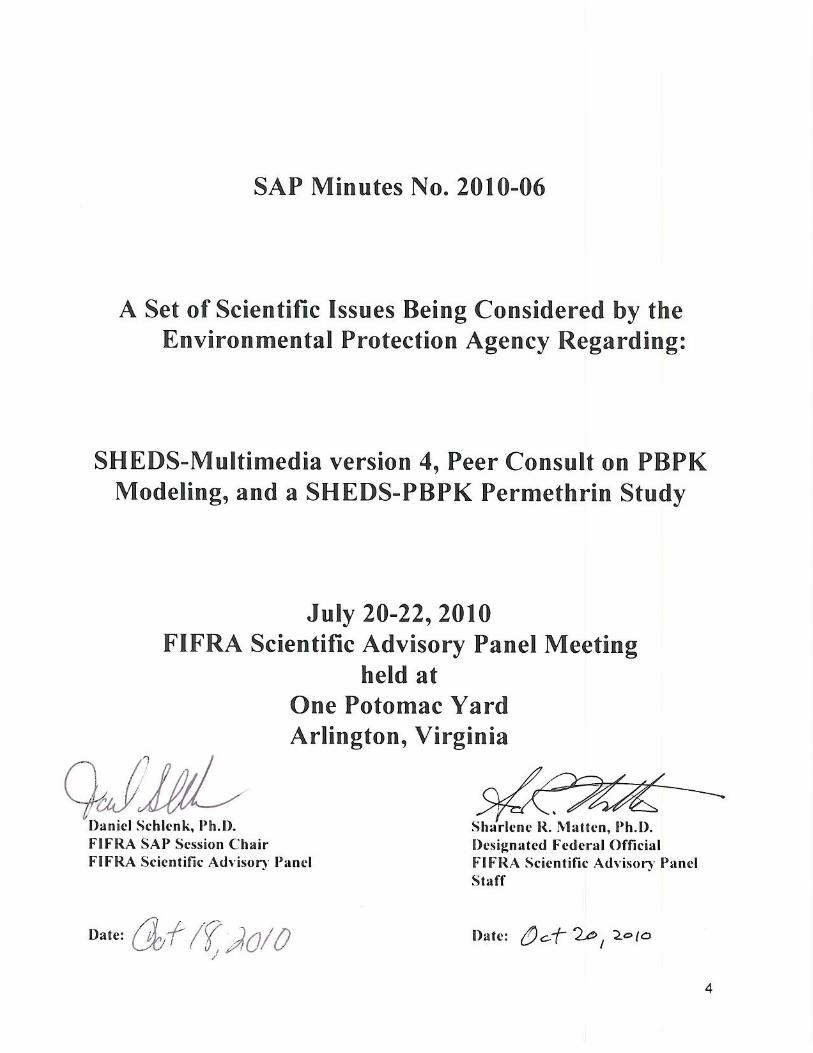
SAP Minutes No. 2010-06

A Set of Scientific Issues Being Considered by the Environmental Protection Agency Regarding:

SHEDS-Multimedia version 4, Peer Consult on PBPK

Modeling, and a SHEDS-PBPK Permethrin Study

July 20-22, 2010 FIFRA Scientific Advisory Panel Meeting

held at One Potomac Yard Arlington, Virginia

2

NOTICE

These meeting minutes have been written as part of the activities of the Federal Insecticide, Fungicide, and Rodenticide Act (FIFRA), Scientific Advisory Panel (SAP). The meeting minutes represent the views and recommendations of the FIFRA SAP, not the United States Environmental Protection Agency (Agency). The content of the meeting minutes does not represent information approved or disseminated by the Agency. The meeting minutes have not been reviewed for approval by the Agency and, hence, the contents of these meeting minutes do not necessarily represent the views and policies of the Agency, nor of other agencies in the Executive Branch of the Federal government, nor does mention of trade names or commercial products constitute a recommendation for use. The FIFRA SAP is a Federal advisory committee operating in accordance with the Federal Advisory Committee Act and established under the provisions of FIFRA as amended by the Food Quality Protection Act (FQPA) of 1996. The FIFRA SAP provides advice, information, and recommendations to the Agency Administrator on pesticides and pesticide-related issues regarding the impact of regulatory actions on health and the environment. The Panel serves as the primary scientific peer review mechanism of the Environmental Protection Agency (EPA), Office of Pesticide Programs (OPP), and is structured to provide balanced expert assessment of pesticide and pesticide-related matters facing the Agency. FQPA Science Review Board members serve the FIFRA SAP on an ad hoc basis to assist in reviews conducted by the FIFRA SAP. Further information about FIFRA SAP reports and activities can be obtained from its website at http://www.epa.gov/scipoly/sap/ or the OPP Docket at (703) 305-5805. Interested persons are invited to contact Sharlene R. Matten, Ph.D., SAP Designated Federal Official, via e-mail at matten.sharlene@epa.gov

.

In preparing these meeting minutes, the Panel carefully considered all information provided and presented by EPA, as well as information presented in public comment. This document addresses the information provided and presented by EPA within the structure of the charge.

3

TABLE OF CONTENTS

NOTICE ....................................................................................................................................................... 2 PARTICIPANTS......................................................................................................................................... 5 INTRODUCTION ....................................................................................................................................... 9 PUBLIC COMMENTERS ....................................................................................................................... 11 SUMMARY OF PANEL DISCUSSION AND RECOMMENDATIONS ........................................... 12 DETAILED RESPONSES TO CHARGE QUESTIONS ...................................................................... 23 REFERENCES .......................................................................................................................................... 85 APPENDIX I : EDITORIAL COMMENTS REGARDING THE USE OF “SCENARIO” IN THE SHEDS-RESIDENTIAL USER MANUAL ................................................................................... 90

5

Panel Members for the Meeting of the Federal Insecticide, Fungicide and Rodenticide Act Scientific Advisory Panel (FIFRA SAP)

to consider and review SHEDS-Multimedia version 4, Peer Consult on PBPK Modeling, and a

SHEDS-PBPK Permethrin Study

July 20-22, 2010 PARTICIPANTS

FIFRA SAP Chair

Steven G. Heeringa, Ph.D. Research Scientist & Director for Statistical Design University of Michigan Institute for Social Research Ann Arbor, MI

FIFRA SAP Session Chair

Daniel Schlenk, Ph.D. Professor of Aquatic Ecotoxicology & Environmental Toxicology Department of Environmental Sciences University of California, Riverside Riverside, CA

Designated Federal Official

Sharlene R. Matten, Ph.D. US Environmental Protection Agency Office of Science Coordination & Policy FIFRA Scientific Advisory Panel EPA East Building, MC 7201M 1200 Pennsylvania Avenue, NW Washington, DC 20460 Tel: 202-564-8450, Fax: 202-564-8382, matten.sharlene@epa.gov

FIFRA Scientific Advisory Panel Members

Janice E. Chambers, Ph.D., DABT, ATS William L. Giles Distinguished Professor Director, Center for Environmental Health Sciences College of Veterinary Medicine Mississippi State University Mississippi State, MS

6

Gerald A. LeBlanc, Ph.D. Professor and Department Head Department of Environmental & Molecular Toxicology North Carolina State University Raleigh, NC Carey N. Pope, Ph.D. Professor, Head & Sitlington Chair of Toxicology Department of Physiological Sciences Oklahoma State University College of Veterinary Medicine Stillwater, OK Kenneth M. Portier, Ph.D. Program Director, Statistics American Cancer Society National Home Office Atlanta, GA

FQPA Science Review Board Members

Dana Boyd Barr, Ph.D. Research Professor of Environmental Health Rollins School of Public Health Department of: Environmental Health Emory University Atlanta, GA Abby C. Collier, Ph.D. Assistant Professor of Pharmacology John A. Burns School of Medicine University of Hawai’i at Manoa, Kaka’ako campus Honolulu, HI Penelope A. Fenner-Crisp, Ph.D., DABT Private Consultant North Garden, VA Richard Greenwood, Ph.D. Professor of Environmental Science School of Biological Sciences University of Portsmouth Portsmouth, England UNITED KINGDOM

7

Dale B. Hattis, Ph.D. Research Professor The George Perkins Marsh Institute Clark University Worcester, MA Wendy J. Heiger-Bernays, Ph.D. Associate Professor Department of Environmental Health Boston University School of Public Health Boston, MA Sastry S. Isukapalli, Ph.D. Assistant Professor Department of Environmental and Occupational Medicine University of Medicine and Dentistry New Jersey Robert Wood Johnson Medical School Piscataway, NJ Dallas E. Johnson, Ph.D. Professor Emeritus Department of Statistics Kansas State University Manhattan, KS John Kissel, Ph.D. Professor Department of Environmental Health and Occupational Health Sciences School of Public Health and Community Medicine University of Washington Seattle, WA Teresa L. Leavens, Ph.D. Research Assistant Professor College of Veterinary Medicine Center for Chemical Toxicology Research and Pharmacokinetics North Carolina State University Raleigh, NC Chensheng (Alex) Lu, Ph.D. Mark and Catherine Winkler Assistant Professor of Environmental Exposure Biology Department of Environmental Health; Exposure, Epidemiology, and Risk Program Harvard School of Public Health Cambridge, MA

8

Peter D.M. Macdonald, D.Phil., P.Stat. Professor Emeritus of Mathematics & Statistics McMaster University Hamilton, Ontario CANADA William J. Popendorf, Ph.D. Professor Emeritus Department of Biology Utah State University Logan, UT Nu-may Ruby Reed, Ph.D., DABT Staff Toxicologist Department of Pesticide Regulation California EPA Sacramento, CA

9

INTRODUCTION The Federal Insecticide, Fungicide, and Rodenticide Act (FIFRA) Scientific Advisory Panel (SAP) has completed its review of the Agency’s analysis of SHEDS-Multimedia version 4, Peer Consult on PBPK Modeling, and a SHEDS-PBPK Permethrin Study. Advance notice of the SAP meeting was published in the Federal Register on April 30, 2010. The review was conducted in an open Panel meeting held on July 20-22, 2010 at One Potomac Yard, Arlington, Virginia. Materials for this meeting are available in the Office of Pesticide Programs (OPP) public docket or via Regulations.gov, OPP Docket: EPA-HQ-OPP-2010-0383. Daniel Schlenk, Ph.D. chaired the meeting. Sharlene Matten, Ph.D. served as the Designated Federal Official. Stephen Bradbury, Ph.D., Director, Office of Pesticide Programs (OPP) and Steven Knizner, Associate Director, Health Effects Division (HED), OPP provided opening remarks at the meeting. Presentations of technical background materials were provided by the following members of the Office of Research and Development (ORD): Andrew Geller, Ph.D., Valerie Zartarian, Ph.D., and Rogelio Tornero-Velez, Ph.D., National Exposure Research Laboratory (NERL); Jimena Davis, Ph.D., and R.Woodrow Setzer, Ph.D, National Center for Computational Toxicology (NCCT). Additional technical assistance during the meeting and in the compilation of the background documents was provided by the following individuals: Jianping Xue, M.D. and Kristin Isaacs, Ph.D., ORD-NERL; David Miller (Chief), Jeff Evans, David Hrdy, Steven Nako, Ph.D., Aaron Niman, Chemistry and Exposure Branch, HED, OPP; Graham Glen, Ph.D. and Luther Smith, Ph.D., Alion Science Technology, Inc. (contractors for U.S. EPA, ORD). The Food Quality Protection Act (FQPA) amended laws under which EPA evaluates the safety of pesticide residues in food. Section 408(b)(2)(D)(v) and (vi) of the Federal Food, Drug, and Cosmetic Act (FFDCA) as amended by FQPA, specifies that, when determining the safety of a pesticide chemical, EPA shall consider aggregate exposure (i.e., total dietary (food and water), residential, and other non-occupational) and available information concerning the cumulative effects to human health that may result from exposure to other substances that have a common mechanism of toxicity. Aggregate assessments account for multiple sources and routes of exposure for a single chemical. FQPA-mandated cumulative assessments combine exposures and doses to two or more chemicals that share a common mechanism of toxicity. OPP and ORD have collaborated on scientific efforts to inform the Agency’s anticipated pyrethroid cumulative risk assessment (CRA). This FIFRA SAP review is part of the Agency's ongoing process to enhance probabilistic exposure, dose, and risk assessments, and OPP's ongoing efforts to consider available probabilistic exposure and dose models to address requirements mandated by FQPA. ORD and OPP scientists have developed new approaches for CRA which have been incorporated into the Agency’s SHEDS-Multimedia (Stochastic Human Exposure and Dose Simulation) computer model and software. SHEDS-Multimedia (http://www.epa.gov/heasd/products/ sheds_multimedia/sheds_mm.html) is a physically based, probabilistic model that predicts -- for user-specified population cohorts -- exposures incurred via eating contaminated foods or drinking water, inhaling contaminated air, touching contaminated surface residues, and ingesting residues from hand-to-mouth or object- to-mouth activities. It can simulate aggregate or cumulative exposures over time via multiple routes of exposure (dietary and non-dietary residential) for multiple types of chemicals and scenarios. To

10

do this, it combines information on chemical usage, human activity data e.g., from Consolidated Human Activity Database (CHAD; www.epa.gov/chadnet1) time/activity diary surveys and videography studies), environmental residues and concentrations, and exposure factors to generate time series of exposure for simulated individuals. One-stage or two-stage Monte Carlo simulation is used to produce distributions of exposure for various population cohorts (e.g., age/gender groups) that reflect the variability and/or uncertainty in the input parameters. While the core of SHEDS-Multimedia is the concentration-to-exposure module, there are various options (e.g., built-in simple source-to-concentration module, user-entered time series from other models or field study measurements) for obtaining concentration inputs. SHEDS-Multimedia also includes a simple built-in pharmacokinetic (PK) model. In addition, SHEDS-Multimedia exposure outputs can be used as inputs to more sophisticated physiologically based pharmacokinetic (PBPK) models which can, in turn, be used to model and estimate tissue burden and urinary concentrations of chemicals through class-oriented approaches. The combined exposure- and dose-modeled outputs will be compared against real-world biomonitoring data, and will be integrated with corresponding effects research. An earlier version of the SHEDS-Multimedia model (version 3) was originally presented to the SAP for review in August 2007 (http://www.epa.gov/scipoly/SAP/meetings/2007/081407_mtg.htm). In that version, only the aggregate residential module of SHEDS-Multimedia was operational, and then only for post-application exposures (i.e., pesticide applicators were not considered). In that 2007 meeting, the SAP reviewed the aggregate residential (post-application only) version of SHEDS-Multimedia (version 3), as well as conceptual plans for the SHEDS dietary module and for the PBPK modeling. The purpose of the July 2010 SAP meeting was to request input from the SAP on the updated versions of the SHEDS-Multimedia and PBPK models since 2007. Specifically, the FIFRA SAP was asked to review: (i) the dietary module of SHEDS-Multimedia version 4, including algorithms, inputs, and results illustrated with a permethrin case study; (ii) the residential module of SHEDS-Multimedia version 4, including algorithms, inputs, and results illustrated with a permethrin case study; (iii) the SHEDS-Multimedia version 4 aggregate (dietary and residential modules combined) permethrin case study, including algorithms, inputs, and results; (iv) update on PBPK modeling since the 2007 SAP, and approaches for and results of linking SHEDS-Multimedia with PBPK models, illustrated with a permethrin case study; and (v) plans for a mini-cumulative (2-3 chemicals) cumulative pyrethroids assessment, including proposed methodologies using linked SHEDS-Multimedia and PBPK models. The Panel members were asked to focus on non-chemical-specific default inputs at the meeting. A permethrin case study was presented for model illustration and evaluation purposes only. The Panel was not asked to assess permethrin outputs. Overall, the SAP’s recommendations will assist the Agency in its specific efforts to assess the cumulative risk of pyrethroids and support a more generalized CRA approach that can be applied to other chemicals in the future.

11

PUBLIC COMMENTERS Oral statements were presented by: David Kim, Ph.D., Syngenta Crop Protection, Inc., on behalf of the Pyrethroid Working Group (PWG) Written statements were provided by: Gary Mihlan, Ph.D., CIH; Chair, Modeling Committee, on behalf of the PWG:

12

SUMMARY OF PANEL DISCUSSION AND RECOMMENDATIONS

Issue 1: Usability aspects of the SHEDS Dietary Module (SHEDS-Dietary v.1.0) and the

SHEDS Residential Module (SHEDS-Residential v.4.0) Question 1-1: What, if any, difficulties were encountered in loading or running the SHEDS-Dietary software? The general consensus of the Panel was that the SHEDS-Dietary module was not a program for the naïve user. The program is significantly more complex than the SHEDS-Residential v. 4.0 module (SHEDS-Residential) and harder to implement. Successful users need to invest time reading the User Guide and more than a couple of hours in understanding how the software works. Users need a good understanding of the databases involved and some insight into where the SHEDS-Dietary v.1 module (SHEDS-Dietary) stores the particular data for a run. Many of the Panel indicated that problems seemed to arise from issues with intermediate files. For the SHEDS-Dietary module to run properly, all of the intermediate files must be correctly named, constituted, and stored in the expected locations. The Panel recommended that the EPA developers consider the option of changing the storage of run files from folders organized according to type, as is currently implemented, to having all files associated with a run stored in a specific run folder. Such a structure would help users and EPA support personnel to identify more easily what might be causing errors on a specific run. The Panel provided several suggestions to improve loading and/or running the SHEDS-Dietary module. Question 1-2: Please comment on the organization, clarity, completeness, and usefulness of the SHEDS Dietary Technical Manual and the User Guide. Please provide any suggestions for improvement. The Panel stated that the Technical Manual and User Guide were generally well-written and understandable. Both documents assume a minimal level of understanding about dietary exposure analysis on the part of the user. Individuals who are not as familiar with the SAS1

software and dietary exposure analysis would need to spend significant time with the program to understand its operation and the appropriate input data for their specific assessment. Both documents made good use of links to other supporting documents on the internet. There was, however, a general consensus that the User Guide needed to be simplified and the Technical Manual expanded to include more topics. Many of the recommendations of the August 2007 SAP (SAP, 2007) on the restructuring of the SHEDS-Residential User Guide and Technical Manual did not seem to have been applied to the SHEDS-Dietary documentation. Panel members suggested that the SHEDS-Dietary Technical Manual follow the content structure of the SHEDS-Residential Technical Manual. The Panel recommended the creation of a much shorter "Quick Reference Guide to the SHEDS-Dietary Model."

1 SAS and all other SAS Institute Inc. product or service names are registered trademarks or trademarks of SAS Institute Inc. in the USA and other countries. ® indicates USA registration.

13

Question 1-3: Please comment on the organization and usability of the SHEDS-Dietary GUI (Graphic User Interface), and whether additional changes would be helpful the Dietary SHEDS. Many on the Panel found the GUI for the Dietary SHEDS application to be logical, intuitive, and easy to navigate. Only a few of the dialogs have buttons that cannot immediately be seen without scrolling. Interacting with the dialogs is straightforward and output was easy to obtain and view. A number of suggestions were made by the Panel. Question 1-4: What, if any, difficulties were encountered in loading or running the software for SHEDS-Residential software? The Panel stated that the SHEDS-Residential v.4 module is more mature than the SHEDS-Dietary v.1 module and has benefited from previous review by the SAP in August 2007. Still, the Panel did encounter problems during the installation and running of the program. Some Panel members were not familiar with installing the SAS software and hence, encountered several problems during that process, in particular, requests to reassign a computer’s pre-existing .log and .csg file types to the SAS software configuration. These Panel members indicated that there was insufficient guidance as to the minimal SAS software configuration needed to run SHEDS-Residential or SHEDS-Dietary. The SAS software comes with over a dozen modules and some institutions may not maintain licenses for all them. The Panel recommended that guidance be offered on which specific SAS software modules are required for successful running of the SHEDS tools, e.g., SAS/BASE, SAS/STAT, SAS/GRAPH. Users who do not have the appropriate SAS modules installed could find that SHEDS fails to run. The Panel initiated a discussion of whether SHEDS tools migrate from SAS onto an open-source system such as the R-language environment. Question 1-5: Please comment on the organization, clarity, completeness, and usefulness of the SHEDS Residential Technical Manual and the User Guide? Please provide any suggestions for improvement. Both the SHEDS-Residential Technical Manual and User Guide were generally well-written and understandable. There is a fair amount of jargon in the documents which is acceptable if the user is experienced in residential risk assessment and exposure modeling. Both documents assume a modest level of understanding about residential exposure analysis on the part of the user – knowledge not provided in either document and not mentioned as a prerequisite. Both documents seem to have been written for users familiar with SAS software and experienced in obtaining data for their specific assessment. The Panel identified a number of undefined or inconsistently defined terms. The Residential Technical Manual was close to what many Panel members expected of a technical manual. On the other hand, the SHEDS-Residential Technical Manual was not particularly helpful in discussing issues related to soil ingestion. A number of Panel members recommended the creation of a “Quick Reference Guide” for users less inclined to read the entire Users Guide. Chapter 6 of the User Guide was suggested as coming close to a SHEDS-Residential Quick Reference Guide.

14

Question 1-6: Please comment on the organization and usability of the SHEDS Residential GUI (Graphic User Interface), and whether additional changes would be helpful for the Residential SHEDS. Many on the Panel found the SHEDS-Residential GUI significantly improved from the previous version reviewed by the SAP in August 2007 and to be logical, intuitive, and easy to navigate. The interface was excellent and interacting with the dialogs is straightforward. Only a few of the dialogs have buttons that cannot immediately be seen without scrolling. Output was easy to obtain and view, although, at least one Panel member pointed out that the plots of distributions functions and other graphical summaries (e.g., box and whiskers plots) offer no option to change the Y-axis to a log scale. These panelists preferred to use the natural log scale as the default because many of the current plots lack detail for observations clustered near zero. The user interface for dose specification that included a nice graphical presentation of the specified distribution was pointed out as being a really useful feature that should be considered for all dialogs where users must specify distributions. This functionality provides the user an easy tool for checking whether the distribution as specified meets user expectations. Issue 2: SHEDS Completeness and Technical Aspects Question 2-1: Exposure Algorithms and Model Components: Q2-1(a): Please comment on whether the exposure algorithms and model components as described in the Technical Manuals are science based and technically correct for the Dietary module. Q2-1(b): Please comment on whether the exposure algorithms and model components as described in the Technical Manuals are science based and technically correct for the Residential module. The Panel agreed with the general modeling approach of SHEDS-Multimedia reliance on probabilistic sampling of a large number of random variables and subsequent aggregation of exposure events and exposures. The structure of the model is relatively stable because the model processes a large amount of data (representing a large number of individuals) using a set of relatively straight-forward rules and calculations. Therefore, ensuring model correctness involves ensuring that correct sets of inputs and parameters are provided in order to define specific exposure scenarios. However, the Panel had several major concerns with regard to the currently used exposure algorithms in both of the SHEDS-Dietary and SHEDS-Residential modules.

1) The SHEDS-Residential model currently lacks the flexibility needed to estimate

[dermal] exposures resulting from formulations of permethrin (often in combination with DEET) used to treat clothing, furniture, and sleeping bags. Therefore, the Panel recommended that the Agency re-evaluate how this potentially important exposure pathway might be addressed in the model.

2) The Panel indicated that the Agency had addressed the major issues regarding the

handling of drinking water exposures raised by the August 2007 SAP Panel (SAP

15

2007) in the SHEDS-Dietary model. However, some aspects of infant exposure via drinking water remain problematic. For example, the model may not be able to capture such localized higher concentrations of pyrethroids in agricultural communities.

3) The Panel stated that the dust ingestion protocol used by the Agency needs further

explanation. The SHEDS-Residential Technical Manual relied on data from an unpublished manuscript by Özkaynak et al. (2010, in press) entitled, “Modeled Estimates of Soil and Dust Ingestion Rates in Children” to parameterize the model. However without these data, the Panel was limited in its ability to understand the approach used by Özkaynak et al. (2010, in press) for model evaluation or how the treatment of dust and soil was incorporated in to the model. The Panel recommended additional evaluation of the dust matrix and suggested that more empirical data in this area be collected rather than performing a new statistical evaluation of older data.

4) The SHEDS-Residential model currently provides exposure estimates at a national

level, and has been evaluated using national level data. Even though this may be adequate for providing good national estimates, the model may still significantly over- or under-estimate region-specific exposures which depend on factors such as seasonality, climate, crop specificity (agricultural use) or drinking water quality. The Panel recommended that the model should take into account different geographical locations to more specifically look at exposure patterns based on where a simulated individual resides.

5) The Panel stated that the Agency should clearly describe in the Technical Manual

how the “Food Commodity Intake Database” (FCID) is compiled, and how SHEDS Dietary utilizes “recipes” in the FCID for simulating dietary intake of pesticides.

Question 2-2: Residential and Dietary Technical Aspects Q2-2(a): Please comment on whether the annotated code for the SHEDS residential model (i) is sufficiently clear such that the algorithms can be followed and understood; and (ii) whether the algorithms defined in the Residential Technical Manual are consistent with those present in the code. In what ways might the code, its annotations, or the description in the Technical Manual be improved? Please consider in particular the new components of the code (i.e., added or modified since the 2007 SAP) as detailed and described in Section 1.6 of the Residential Technical Manual. Q2-2(b): While the underlying SAS code [of SHEDS-Dietary Version 1] has not at this time been fully annotated and/or is not as “reader-friendly” as the residential code, does the Panel have any comments or suggestions on the structure or form of the code or ways in which the code may be improved? Can the Panel identify any apparent discrepancies between the calculations described in the Dietary Technical Manual and the algorithms operating in and described by the SAS code?

16

The Panel reviewed the code in SHEDS-Residential version 4 and compared it to SHEDS-Residential version 3 reviewed by the August 2007 SAP. Even though the Panel could not assure all the code was correct in version 4, Panel members agreed that the steps in the “Level 1 Quality Assurance Project Plan” were thorough and satisfactory, and if followed, would achieve the required standard for SHEDS Multimedia applications. The Panel reviewed the dietary code and found the code well annotated. In general, the algorithms and code appear technically correct. Overall, many members of the Panel supported the decision to continue using the SAS software because of its significant database capabilities, although the benefits of a potential migration to an open-source programming platform and running the SHEDS-multimedia program via the web were also discussed. The Panel provided specific comments and suggestions on a number of coding and programming aspects of the SHEDS-multimedia modules.

1) Potential migration to an open-source programming platform (e.g., from SAS code to R language). Some Panel members agreed that the requirement of a SAS software license imposes substantial challenges in the use of the SHEDS-Multimedia program. As an alternative to SAS software, some Panel members suggested that it might be feasible to run SHEDS-multimedia remotely via a website hosted by the Agency rather than downloading the software from the web and run SHEDS-Dietary or SHEDS-Residential on a local computer. Another alternative suggested was the use of the open-source R language (R Development Core Team, 2009) rather than SAS code. The rationale for this is that all the functionality of SAS code needed for SHEDS is available in R language and the migration from SAS code to R language could be straight-forward. In fact, the PBPK modeling system accompanying the SHEDS system has been coded in R language. Panel members pointed out that a large number of bioinformatics and computational toxicology researchers within the Agency use R language.

2) Organization of the program code structure (file and folder structure). The Panel

stated that many of the comments from the August 2007 SAP concerning the SHEDS-Residential model (then called SHEDS-Multimedia version 3) are directly applicable to the SHEDS-Dietary model version 1.

3) SAS coding practices. The overall SAS code contains about 15,000 lines of code, with

the main exposure model calculations consisting of a few hundred lines. The Panel found it relatively easy to follow the code and understand the calculations. The current code structure with the outer loop representing multiple chemicals is appropriate, and is easy to follow. However, the Panel had several specific comments and suggestions to improve the coding practices.

4) Making the code available. Some Panel members expressed concern about making

the code publicly available because it may allow arbitrary modifications of the code by different users and may result in incompatible versions of SHEDS code.

5) Sampling approaches. Currently, the SHEDS system avoids unrealistic exposure

scenarios by using truncations of underlying distributions (e.g., for probabilities of

17

contacts, distributions of concentration residues). This may affect some exposure scenarios that are realistic, but lie on the extremes of the distributions.

6) Ability to run the model in a deterministic mode. One option recommended by the

Panel was to run the SHEDS code in a “deterministic mode” where the sample values of different parameters can be specified. Then, the code can be used to reproduce exposures under values of input parameters that correspond to tails of distributions or high exposure cases.

7) Simulation of population groups. The Panel suggested that future versions of the

SHEDS program have the ability to assign simulated people to groups who are exposed to a similar pesticide environment. This suggestion was also made by the August 2007 SAP (p. 31 of the background document, “Agency’s Response to the 2007 SAP Comments,” found in Regulations.gov, OPP Docket: EPA-HQ-OPP-2010-0383). ). For example, residential scenarios could comprise residents in the same apartment building, dormitory, or institutional setting.

8) Modeling of dermal absorption. Panel members stated that the approach used to

evaluate dermal dose was inadequate. Specifically, the modeling of dermal absorption as a first order process using rate constants estimated under high load conditions and then extrapolated to low load conditions is inappropriate (Kissel 2010).

Issue 3: Strengths and Limitations of PBPK Approaches Question 3-1: Please comment on the strengths and limitations of the pharmacokinetic modeling approach for pyrethroids with added attention to the PBPK structures for interpreting aggregate exposure data from SHEDS. The Panel agreed with the Agency’s approach to develop a generic PBPK model structure with chemical specific parameters and noted that EPA has made considerable progress since the August 2007 SAP meeting in its PBPK modeling approach for pyrethroids and use of aggregate exposure data from SHEDS (Residential and Dietary modules). The ability to link the exposure information from SHEDS to dose-metrics predicted by the PBPK model is a highly desirable step and marks a substantial improvement over the compartmental modeling used in prior versions. Such linking of these two models should avoid creating inappropriate overlaps that can occur by maintaining separate models, and linking more individual data between these models also has statistical advantages. However, the Panel also pointed out that separate models have practical advantages both during model evaluation, testing and ultimately to diverse users. Thus, the Panel recommended that a seamless, but optional linkage be created between the SHEDS exposure and PBPK components so that they can be run either in tandem or separately. The Panel discussed both the strengths and limitations in the current PBPK modeling approach and urged that the plausibility of the model be built as much on relevant biological processes as mathematical/statistical criteria. As discussed below, Panel members were not able to adequately assess the PBPK structures that were presented at the meeting since these materials were not made available with sufficient lead-time.

18

Question 3-2: Please comment on the Bayesian approach outlined here for calibrating the PBPK model against rodent PK data, including the use of computational and in vitro methods to develop priors for chemical-specific parameters. The Bayesian approach used by the EPA for model-data fusion with techniques such as Bayesian Markov Chain Monte Carlo (MCMC) methods is currently the best approach for estimating model parameters, since it incorporates prior information, model refinements, and new data. Because SHEDS and the PBPK models can be run in a parallel mode (either at the Bayesian MCMC chain level, or by submitting simulations for subgroups of individuals to different computers), the generally intense requirement of computational resources is minimized. However, there are still some relatively straight-forward improvements in the modeling strategy that can be achieved. For example, sensitivity analyses should be performed to identify important parameters for focusing future modeling efforts and in vitro experiments. Some of the assumptions for extrapolating between in vitro and in vivo data and among species do not have sufficient supporting data. The Panel also recommended that the Agency explore the aspect of Bayesian model selection and model averaging when multiple alternative model structures are possible (Toni and Stumpf, 2010). One Panel member recommended Appendix A of the IRIS Toxicological Review of Trichloroethylene (currently under external review by the US EPA Science Advisory Board) as an example of integrating in vitro with in vivo data and a documented Bayesian approach to calibrating a PBPK model against mice and rat data (available at http://cfpub.epa.gov/ncea/cfm/recordisplay.cfm?deid=215006). Question 3-3: Please comment on the approach used to characterize the animal-to-human extrapolation, including the uncertainty of the extrapolation. Consistent with feedback for Charge Question 3-1, the Panel expressed a need for more information to adequately assess the modeling work including the animal-to-human extrapolation. One recommendation by the Panel was to have the background documents include more explicit mathematical descriptions. For example, a metabolic rate for humans could be characterized mathematically as the sum or product of factors to represent the relationship between the rat rate and the human rate. If the human rate can be conceptualized as the product of a factor (X), which can be estimated directly from the rat, and a multiplier (Y), which will be used to scale the rat value to humans, then there can be a more productive discussion on how well (X) is informed from rat studies and how well (Y) is characterized from known physiology principles, such as allometric relationships between rates and individual or organ sizes (e.g., the ¾ power relationship). In addition, as noted in Charge Question 3.2, the Panel recommended that the Agency conduct a sensitivity analysis to determine which parameters in the model are drivers, and what additional empirical data are needed to fill gaps that have the greatest impacts on the model. The Panel recommended that the Agency apply methods to assess the gamma parameter used for the rat to human in vitro and in vivo extrapolations. A rigorous review of the published literature should identify biological properties relevant to the species differences, which could then assist EPA in filling some data gaps until empirical rat or human data (in vivo and in vitro) can be collected. These data could then be used to place bounds on the uncertainty by evaluating the distributions of the parameters used in the analysis. The Panel discussed several specific aspects of the animal-to-human extrapolations in the modeling.

19

1) Oral absorption. The Panel commented that there is a lack of information on how

the oral absorption rate was extrapolated across species, as well as from in vitro to in vivo scenarios.

2) Tissue distribution-diffusion limitation (i.e., permeability-surface area coefficients).

One particular area of uncertainty discussed by the Panel was how the diffusion limitation was included in the model with regard to human versus rat values for the permeability-surface area coefficients of the various tissues.

3) Lactational exposure. The Panel indicated that additional empirical data on

lactational exposure in rodents should be collected. 4) Low tissue concentrations below the Km. The Panel raised a concern with the

assumption of low tissue concentrations of pyrethroids, particularly at concentrations that are below the Km of the metabolic enzymes in all tissues, e.g., in the placenta of a pregnant woman and in a young child (i.e., nursing or post weaning).

5) Piperonyl butoxide impact. The Panel commented that if piperonyl butoxide is able

to inhibit or modify the human enzyme systems, then it is plausible that the rates and amounts of parent and metabolites would be different than in the case of neat compound alone.

Question 3-4: Please comment on the plausibility and limitations of model-predicted dose-metrics, such as area under the curve (AUC), peak tissue values, time above a toxicological threshold, or AUC above a toxicological threshold, in analyzing animal dose-response data and in extrapolation to humans. The Panel recommended flexibility in the model structure and in the chosen dose-metric. A carefully calibrated and validated pyrethroid PBPK model could be used to estimate any of the proposed dose-metrics. The Panel considered the array of dose-metric options listed by the Agency and expressed preference for either “simple peak concentrations” or “AUC” as dose-metrics. There was not enough information about the mode(s) of action of pyrethroids to postulate a specific “toxicological threshold” or “the time over the threshold” values. The Panel stated that it was not sufficient to rely on a small set of dose-metrics for cross-species extrapolation until an integrated pharmacokinetic/pharmacodynamic model has been developed. The model should be constructed to be flexible enough to incorporate a wide array of potential dose-metrics and should retain the ability to generate time-dependent variation. As pointed out by one Panel member, the endpoints will determine the correct metric. Before any specific dose-metric (or set of dose-metrics) can be chosen, the Panel indicated that the limitations in the PBPK model outlined in Charge Question 3.1 will need to be addressed, including the effects of age, diseases such as obesity and diabetes, gender, pregnancy and body weight. Use of the 70-kg male human may not be appropriate to assess internal exposure to pyrethroid pesticides across the population.

20

Question 3-5: The presentation described methods for addressing uncertainty in model parameters and extrapolation from animals to humans. What other important sources of uncertainty need to be addressed for either the SHEDS exposure model or the PBPK model? The Panel outlined several areas of uncertainty in the data used for model development, e.g., the influence of censored data on parameter estimates, pharmacodynamic differences among species and individuals, and techniques for addressing individual uncertainty and distributions in various age groups. In addition, the Panel pointed out that there is also uncertainty in the “form of the model” that should be considered. As new information becomes available some of the PBPK model compartments might need to be expanded. This may be particularly important as the generic model grows in utility to accommodate more chemicals or the need to incorporate more complexity in specific compartments. The approach for uncertainty analysis currently involves the aggregation of results from SHEDS-Residential (or SHEDS-Dietary) for each individual, and using them as inputs and parameters for doing PBPK simulation. The Panel indicated that of the various sources of uncertainty currently not addressed by the SHEDS and the PBPK model, the two major types are:

1) Uncertainty due to a limited number of samples. Specifically, the tails of the distributions may not be adequately captured by a small number of uncertainty samples (typically of the order of 100 used in the SHEDS simulations).

2) Model/structural uncertainties. These uncertainties will occur when multiple alternative formulations are available. One approach to reduce this uncertainty involves the application of Bayesian model selection and model averaging techniques (Toni and Stumpf, 2010).

Issue 4: Model Evaluation Question 4: Please comment on the process used to evaluate SHEDS. Are the above listed ways in which SHEDS was evaluated appropriate? In what ways could they be improved? Are there other methods through which the model should or can be evaluated? Are there other data (e.g., biomonitoring data, duplicate diet data) that the Panel is aware of through which the SHEDS model can be compared? The Panel agreed that linking a probabilistic exposure model (SHEDS) with a PBPK model provides a unifying approach that will potentially furnish a way of assessing new compounds of concern or combinations of compounds. Ideally, the performance of SHEDS in the simulation of exposures should be evaluated against sound external data and modelling that can provide a gold-standard benchmark; however, in the opinion of the Panel, such a gold-standard is not currently available. Rather than focussing on whether the approaches are appropriate or not, the Agency should use this opportunity to examine the results from the evaluation to examine in detail where discrepancies and agreement exist. Further analyses would provide greater clarity in the understanding of the outcomes of the various comparisons. The Panel encouraged the Agency to continue their ongoing efforts to evaluate the model system, and to define the reliability of the model.

In general, the PBPK model comparisons described by the Agency provided useful information on the application of the full model. In the case of permethrin, the Agency concluded that the

21

model evaluation provided confidence in the SHEDS-Dietary model. However, in some areas, there is a lack of similarity between the model prediction and the measured data, and these disparities should be examined in detail.

Issue 5: SHEDS-PBPK Permethrin Case Study Question 5-1: EPA has used a pyrethroid insecticide, permethrin, as a case study to link the SHEDS exposure model with PBPK modeling in order to be able to better interpret and understand exposure data in terms of dose and target-organ dose and assist in refining exposure estimates and associated risk. Please comment on the approaches and offer alternatives and suggestions for:

a) linking dietary consumption diaries and residential activity information (e.g., key factors used for matching food consumption and activity pattern diaries such as caloric consumption);

b) quantification of dietary vs. residential contribution, including relative contribution of residential exposure pathways (dermal, inhalation, hand-to-mouth, object-to mouth);

c) D[iversity] and A[utocorrelation] [D & A] longitudinal diary assembly approach (Glen et al., 2007, reviewed for residential module by 2007 SAP);

d) identifying significant contributors at upper percentiles of dietary exposure; and e) techniques and utility of bootstrapping approaches for quantifying uncertainty and its

interpretation. The Panel agreed that the permethrin case study to link the SHEDS exposure model with PBPK modeling was useful and indicated an overall correspondence of predicted and observed biomarker values that were better than could usually be expected. The Panel concluded that the overall accuracy of the SHEDS/PBPK predictions for high percentiles seemed to be good when compared with existing lab and survey-based databases; however, further research is needed where the agreement between model predictions and empirical data was not as good. For rats (Figure 3 of the Agency background document by Tornero-Velez et al., 2010a), the agreement among predicted peak tissue concentrations was very good (generally within about a factor of two), while the agreement among 48-hour brain levels was not (often under-predicting by about a factor of 10). The Panel indicated that an investigation of whether the weaker match at longer times is important depends on how the modeled data will be used by EPA. The mean and upper percentiles of the urinary excretion predicted for humans shown in Figures 10-11 of the Agency background document by Tornero-Velez et al. (2010a) generally match NHANES data within even less than a factor of two. The Panel commented that many of the results presented by the Agency of multiple exploratory approaches to assess the validity and robustness of this model were illuminating; however, the variations in the assumptions or modifications made to accommodate these approaches (e.g., the handling of dietary residues less than the LOD, skin loading and absorption, and the amount and permeability of clothing) can give the impression of an ad hoc process used to inform the modeling. The Panel indicated that the Agency should strive to rationalize the differences among the various test conditions and assumptions to make them more uniform (or thoughtfully assess the impact of unavoidable differences).

22

Question 5-2: Please comment on whether the model evaluation approach comparing the linked SHEDS-PBPK dose predictions and NHANES (National Health and Nutrition Exams Survey) biomonitoring data is reasonable. Are there other model evaluation methods that the Panel would like to see the Agency perform? The Panel concluded that the comparison between SHEDS-PBPK dose predictions and NHANES biomonitoring data is reasonable, but pointed out numerous caveats concerning limitations and nuances, within the existing databases (especially, but not exclusively, for NHANES) that make them less than a “gold standard.” Some obvious limitations are the impact of censoring that prevents the accurate prediction of dietary 50th percentiles and the fact that the censoring cut-points are not a constant across groups. Less obvious limitations include the sampling schedule, right choice of biomarkers of exposure, artifact contamination, preformed metabolites in the environment, and short half-lives of pyrethroids. The Panel recommended that the raw data from NHANES be used rather than the Center for Disease Control’s (CDC’s) Report on Human Exposure to Environmental Chemicals (www.cdc.gov/exposurereport) because the summary data have several limitations. The Panel also urged caution when assuming NHANES data are reflective of average US population-based exposures over all seasons. The Panel discussed the findings of Barr et al. (2010) regarding predictors or correlates of pyrethroid metabolite (e.g., 3-PBA) concentrations within NHANES. Question 5-3: Please comment on the approaches presented to extend the SHEDS-PBPK Permethrin Case Study to include exposure to cypermethrin and cyfluthrin. Furthermore, please advise on other methodologies (e.g., cross-sectional vs. longitudinal), exposure scenarios, chemicals, and datasets which may be useful to consider in assessing SHEDS-PBPK simulations The Panel concluded that the Agency’s underlying concept and the tools (i.e., PBPK model in combination with SHEDS) were fundamentally sound. However, further extending the PBPK-SHEDS model to fit other pyrethroids will require adding increased complexity to the model to cope with a myriad of issues. While most panelists agreed that such an expanded model would be of great value, such an expansion may be feasible only for levels of exposure sufficiently low such that interactions, saturation, and induction are avoided. To model exposures beyond the normal low chronic levels to include high percentiles or acute effects will increase the complexity of the model and the challenge of developing it. The Panel indicated that the Agency provided a case study of a simple, single chemical analysis of a model that is both elegant and parsimonious, and able to utilize SHEDS output as a separate component to its modeled clearance. On the one hand, the Agency’s plans to extend this PBPK model for mixtures of chemicals assessed simultaneously is to be applauded since ultimately this represents real-world environmental exposure-ADME considerations. However, the Panel identified a number of issues that should be considered further before using the model presented in this manner.

23

DETAILED RESPONSES TO CHARGE QUESTIONS Issue 1: Usability aspects of the SHEDS Dietary Module (SHEDS-Dietary v.1.0) and the

SHEDS Residential Module (SHEDS-Residential v.4.0) A. SHEDS DIETARY Question 1-1: What, if any, difficulties were encountered in loading or running the SHEDS-Dietary software?

Panel Response

The general consensus of the Panel was that SHEDS-Dietary module was not a program for the naïve user. The program is significantly more complex than SHEDS-Residential v. 4.0 module (SHEDS-Residential) and harder to implement. Successful users need to invest time reading the User Guide and more than a couple of hours in understanding how the software works. Users need a good understanding of the databases involved and some insight into where the SHEDS-Dietary v.1 module (SHEDS-Dietary) stores the particular data for a run. Many of the Panel indicated that problems seemed to arise from issues with intermediate files. For the SHEDS-Dietary module to run properly, all of the intermediate files must be correctly named, constituted, and stored in the expected locations. The Panel recommended that the EPA developers consider the option of changing the storage of run files from folders organized according to type as is currently implemented to having all files associated with a run stored in a specific run folder. Such a structure would help users and EPA support personnel to identify more easily what might be causing errors on a specific run. Not all members of the Panel had ready access to the SAS2

software (SAS) and hence were not able to comment on the issue of difficulties in loading the software. About three-quarters of the Panel attempted to load the software and none reported any difficulties. Several panelists were pleased that administrative rights were not required to install the software. One panelist tried to uninstall and re-install the software and was successful. Successful installations were reported for both SAS software, Versions 9.1 and 9.2 of the SAS System for [Unix].

Most of the Panel thought that the current SHEDS-Dietary is appropriate only for relatively sophisticated users. The entire Panel had some experience with running the SHEDS-Dietary software. While some panelists mentioned that use of the program was reasonably intuitive, about half experienced one or more problems with getting the software to do what was expected of it. Reasons for having problems with the software included:

1) Attempting to run the program without first reading the SHEDS-Dietary User Guide.

2 SAS and all other SAS Institute Inc. product or service names are registered trademarks or trademarks of SAS Institute Inc. in the USA and other countries. ® indicates USA registration.

24

2) Expecting the dialogs in the SHEDS-Dietary program to be similar to those in SHEDS-Residential.

3) Making mistakes in the process of returning to previous dialogs. 4) Making it successfully through to the final dialog only to be faced with a run error

requiring examination of the SAS log, which was generally unhelpful, especially for users unfamiliar with SAS software.

A number of panelists who successfully completed one or more of the User Guide examples, indicated changes they would like to see to the various program outputs, recognizing that much of this output is currently dictated by SAS software capabilities. One recommendation was to add titles to any summary or percentile tables as they are printed. This might be easier to implement if the tables were formatted and output as pdf or rtf files. Another was to provide an option to output graphs (with tables and legends) into graphics files using standard graphics formats, such gif or jpeg. One Panelist indicated that when looking at the results of the second case study after previously running the third and fourth case studies they were able to see longitudinal results in the outputs even though longitudinal results were not simulated. For some unknown reasons, the system seemed to be displaying a file from the third case study. Finally, many on the Panel felt that the SHEDS-Dietary interface could benefit from the input of more user focus groups. The Agency explained to the Panel that some of this had been done in the last year. Question 1-2: Please comment on the organization, clarity, completeness, and usefulness of the SHEDS Dietary Technical Manual and the User Guide. Please provide any suggestions for improvement.

Panel Response

General Comments: The Panel stated that the Technical Manual and User Guide were generally well-written and understandable. Both documents assume a minimal level of understanding about dietary exposure analysis on the part of the user - knowledge not provided in either document and not mentioned as a prerequisite. Individuals who are not as familiar with the SAS software and dietary exposure analysis would need to spend significant time with the program to understand its operation and the appropriate input data for their specific assessment. Both documents made good use of links to other supporting documents on the internet. There was, however, a general consensus that the User Guide needed to be simplified and the Technical Manual expanded to include more topics. Many of the recommendations of the August 2007 SAP (SAP 2007) on the restructuring of the SHEDS-Residential User Guide and Technical Manual did not seem to have been applied to the SHEDS-Dietary documentation. Panel members suggested that the SHEDS-Dietary Technical Manual follow the content structure of the SHEDS-Residential Technical Manual. Some Panel members indicated that they

25

would like to explore the capabilities of the new software before reading the detailed User Guide or Technical Manual. These users turn to documentation only when they run into problems. The Panel recommended the creation of a much shorter "Quick Reference Guide to the SHEDS-Dietary Model." The Panel commented that some topics expected to be in the User Guide were found in the Technical Manual and vice versa. There was an expectation that the Technical Manual would be more descriptive than the User Guide, but this was not always the case. For example, the Panel stated that the Technical Manual should describe the purpose and construction of all run-specific files, including the Bridge file. However, the detailed information on the Bridge file is actually in the User Guide where there is not only an overview of the Bridge file structure, but detailed instructions on how to modify the Bridge file. Guidance on how to examine input files directly in SAS using the SAS File Explorer would seem to be a Technical Manual topic, but the introduction to the SAS File Explorer is actually in the User Guide. In addition, there was no discussion of a Batch run capability in the SHEDS-Dietary Technical Manual as there is in the SHEDS-Residential Technical Manual. Specific Comments: SHEDS-Dietary Technical Manual While the Panel noted that the SHEDS-Dietary Technical Manual was generally well-written, many Panel members questioned its completeness and usefulness because they were unsure of the purpose of the document and its eventual audience. As a result, each Panel member judged the document based on their own understanding of what to expect in a technical manual. A couple of Panel members indicated that discussion of the input parameter distributions and parameter prior distributions in the Technical Manual was lacking. In particular, these panelists were looking for insight into which distributions would be more appropriate than others for which parameters and what documents or data sources could be used to inform these decisions. Specific comments: SHEDS Dietary User Guide The Panel agreed that the software installation instructions were clear and easy to follow. Output files and graphs are well discussed and presented. However, examples given were not sufficiently annotated to allow easy implementation by the naïve user. The Panel stated that guidance on what parameter values are acceptable was not adequate in general, and not provided in some cases. A lot of the information provided is possibly more mathematical than many first-time users would be comfortable with. There was general consensus that users should not be required to modify specific files directly, such as the bridge file, to achieve most example run scenarios. For example, users wanting to assign residue to specific foods (e.g., cereal grains) or modify food quantities for a run should not have to select and modify the bridge file. Some Panel members commented that the bridge file is complex and the SHEDS-Dietary model was designed to channel users to use templates from which modifications could be implemented. However, a single mistake in the bridge file modification will produce a run error.

26

Recommendations for the Technical Manual and User Guide 1) The overview diagram for the SHEDS Dietary Interface (Figure 5) gives the impression

the system can be entered from any of the nine (9) menu items displayed on the entry dialog. In fact, only four of the nine items are not grayed out when the entry dialog is initially displayed. Once the “Run File” has been specified, all of the remaining function buttons are available (except, “Add New Crop Group” – a future function). The Panel recommended that this Figure be redesigned to better display both the system functionality and the user interaction paths.

2) Figure and table captions are too short and often non-informative. For example, the

message from Figure 2-2 is not clear and the caption does not help. 3) The limited equations in the document are a mix of words and math symbols which can

lead to confusion. For the equations in the Technical Manual, it is preferable to use either mathematical symbols or corresponding SAS variable names instead of the current use of sentences (e.g., Equation 1 and 2). One suggestion was to replace the math symbol “Σ” with the word "SUM of” in Equations 1 and 2. The sentences can then be used to explain the terms in the equations. The formats used in Equations 2-8 and 2-9 of the SHEDS Residential Technical Manual would be examples of the correct format to use.

4) On page 28, there is a paragraph on Pesticide Use (% crop treated) that seems out of

place because it comes at the end of the 2.3.3 Direct Water Consumption Data section. 5) Section 2.3.5 on Food Residue Data has a paragraph discussing the FDA Total Dietary

Survey with a statement in parenthesis (“not used for pesticides”) followed by a discussion of how the ~280 foods are analyzed for levels of pesticides. The statement in parenthesis is confusing.

6) Section 2.3.6 on Drinking Water Concentration Data has links to OPP environmental

fate models but does not provide much insight into how these models are used in SHEDS-Dietary.

7) Section 2.4 Methods Issues is difficult to understand. An introductory paragraph to

prepare the reader for its contents is needed. 8) On Page 50, some of the sentences have numbers preceding them that should be links

to footnotes. 9) Also on page 50, the meaning of "interaction runs" in the following statement is not

clear: "Sample size: number of simulated persons (number of person days = number of daily food diaries times the number of interactions runs) in age group.”

27

Question 1-3: Please comment on the organization and usability of the SHEDS-Dietary GUI (Graphic User Interface), and whether additional changes would be helpful the Dietary SHEDS.

Panel Response

Many on the Panel found the GUI for the Dietary SHEDS application to be logical, intuitive, and easy to navigate. Only a few of the dialogs have buttons that cannot immediately be seen without scrolling. Interacting with the dialogs is straightforward. Output was easy to obtain and view. A number of suggestions were made by the Panel as listed below.

1) The SHEDS-Residential user interface seemed to the Panel to present a more linear process than did the SHEDS-Dietary user interface. The Panel encouraged the Agency to use the recommendations made by the August 2007 SAP on the SHEDS-Residential interface and apply them to the SHEDS-Dietary module. The Panel suggested that a common user interface structure for both the SHEDS-Dietary and SHEDS-Residential modules be implemented. This intermediate step would integrate both modules into the SHEDS-Multimedia user interface and allow users to easily decide which module to use.

2) For example, the ability to specify alternative folders for storage of simulation files,

activating the Help buttons, having the Run Name displayed prominently in the main window and progress bar corresponding to number of simulations completed/remaining can be adapted from SHEDS-Residential module and used in the SHEDS-Dietary module.

3) Users do not always know what the program had done as a result of filling out a dialog.

In some cases the "Save" button is really a "Save and Return" button and should say so. There is no indication that modified files have actually been saved or notification of the storage location of modified files. Some Panel members reported running into problems of not knowing whether the simulation was actually running. A clear indicator that the simulation is started is needed, such as the progress chart used in SHEDS-Residential.

4) Some Panel members suggested that there may be more buttons than are really needed,

and in some cases the use of drop-down dialog items instead of multiple buttons might enhance the user experience.

5) Error messages (e.g., "File does not exist") should be trapped and shown in a dialog

instead of relegated to the SAS Log file which may be hidden and/or not familiar to the user. Trapping the error may also allow the opportunity to inform the user of potential steps that could be taken to correct mistakes and re-submit.

6) Graphical output and summary tables are more than adequate and easy to obtain. A

number of Panel members noticed that when printed out, graphs and tables did not have adequate captions or titles. This issue was also noted for the SHEDS-Residential output

28

suggesting that developers may need to consider using the SAS Output Delivery System (ODS) capabilities to output graphs in standard graphic file formats (e.g., as jpeg or gif files) and tables in rich text formats. This would also allow for flexibility to incorporate titles and captions.

B. SHEDS RESIDENTIAL Question 1-4: What, if any, difficulties were encountered in loading or running the software for SHEDS-Residential software?

Panel Response

The Panel stated that the SHEDS-Residential v.4 module is more mature than the SHEDS-Dietary v.1 module and has benefited from previous review by the SAP in August 2007. Still, the Panel did encounter problems during the installation and running of the SHEDS-Residential module. Some Panel members were not familiar with installing the SAS software and hence, encountered several problems during that process, in particular, requests to reassign a computer’s pre-existing .log and .csg file types to the SAS software configuration. These Panel members indicated that there was insufficient guidance as to the minimal SAS software configuration needed to run SHEDS-Residential or SHEDS-Dietary. The SAS software comes with over a dozen modules and some institutions may not maintain licenses for all them. The Panel recommended that guidance be offered on which specific SAS software modules are required for successful running of the SHEDS tools, e.g., SAS/BASE, SAS/STAT, SAS/GRAPH. Users who do not have the appropriate SAS modules installed could find that SHEDS fails to run. The Panel noted several other problems they had with using the SHEDS-Residential module. SHEDS-Multimedia tools are open source ware, but the SAS platform on which they run requires the costly administrative license. The Panel initiated a discussion of whether the SHEDS tools should migrate off of SAS onto some other system such as the open-source R environment for statistical computing and graphics (R Development Core Team, 2009). This discussion is covered in greater detail in the response to Issue 2. Users are allowed to change the default file location setting for SHEDS-Residential during installation. However, those Panel members who did choose alternate locations found that the program would not run unless they reinstalled it using the default settings. Upon entering the SHEDS-Multimedia program, the user is first presented with the "Display Issues" screen. Since SAS software program do not normally come up in a screen maximized mode, a number of users were able to view only the "Display Issues" paragraph and the initial "Disclaimer" line. To view the full document the screen has to be maximized. Depending on system specific display options, even with the screen maximized the full document may not be displayed and the user has to scroll down to the end of the text to find the "Continue" button. Once the user has read the "Display Issues" message, it should not be necessary to read it again the next time the program is run. The message is also repeated in the preface of the User Guide. The Panel recommended that a copy of the "Continue" button could also be placed at the top of the file to facilitate rapid entry into the body of the program by more experienced users.

29

One Panel member provided the following detailed comments organized by page number in the Residential User Guide.

Page 16: Users looking to purchase SAS may need to know that either SAS version 9.1 or 9.2 is acceptable, and that both versions are available for 32 or 64 bit systems. The relationship between version number and bit size is not clear in this discussion.

Page 19: Several attempts to use a setup file location that was not the default directory resulted in a Setup error: "Setup was unable to create the directory "C:\Program Files\EPA Multimedia4.00. Error 5: Access denied."

Page 21-23: Most of the User Guide Chapter 4 “The SAS User Interface” was not of use for this first time SHEDS user and in fact was a distraction worth skipping.

Page 21: The first time this reviewer installed the program, screen size was not an issue; however, the second time, the screen opened in less than full size and “Disclaimer” was at the top of the screen. Had prior experience not occurred and the message to maximize the window not been remembered, this reviewer would have been stumped.

Page 21: The "Select the SHEDS-Multimedia Options for this Session" screen is not adequately described in the User Guide. A Help button on the dialog would be useful in providing guidance on how a user will want to answer this question. Shouldn't the dialog be labeled "SHEDS-Multimedia Mode Options" since it is later referred to as the "SHEDS-Mode screen"?

Page 24: The fact that the interface window is labeled “SHEDS Multimedia Main Interface Screen” and the dialog is labeled “SHEDS-Multimedia” is confusing. The text at the bottom of the page reads “After the SHEDS-Mode screen is completed, the main screen will be displayed (Figure 5.2). This is the main interface window

Page 27: Re-label the list box currently named “Select A Defined Run” in Figure 5.3 to the more intuitive (less jargon-like) label “Select an Existing Run” as it is described in the User Guide.

that you will be returned to after completing each main step.” So not only do the text and screen not agree, but the terms Main Screen and main window may refer to two different things. The text should be consistent about referring to "windows" and "dialogs" and possibly avoid talking about "screens".

Page 47-48: The time-frame intended by the authors within SHEDS of the "Number of Applications" in the “Specify Application Dates: Probability” screen must be clarified either within the Guide or the Manual and probably also on the screen. For instance, a user might guess that the number is within the length of the run they are about to simulate, but it could be the number per year (independent of the length of the run), or even the number of times on a given “model determined date.”

Page 59: What does the Background Screen (Dialog?) mean when it refers to “outside surfaces”? Does background only apply to outdoor applications? This appears to be the only place that this term is used in either manual. Part of the confusion may be due to the brevity of Section 5.8.4.

30

Page 71: What does “profiles” (as seen in Figure 5.41) mean? It seems to be used in two contexts here: "10 profiles" and "100 total profiles". Is a profile a simulated person? See further discussion on this term in response to Charge Question 1-5.

Page 73: Some further explanation of the log file would be beneficial, especially if the program fails to run. Trying to decipher error statements without understanding some basic log-file issues was frustratingly unproductive. Improvements may be limited to better descriptions unless changes can be made to the form of the SAS log file (and that form may be intrinsic to the SAS software), see comments related to this file by page in response to Charge Question 1-5.

Page 75: Some confusion was encountered with the sequence by which the various boxes in Figure 5.45 are selected. See comments related to changing this GUI in the corresponding response to Charge Question 1-6.

Page 98: Chapter 6 (the Case Study: Permethrin) was sufficiently clear and uncluttered as to approximate a quick guide. In fact, many of the comments presented herein resulted from using Chapter 6 in just that way.

Page 98: Give each figure a figure number; given the lack of figure numbers, each of the next seven comments refer to a figure listed by the page on which it now resides within the Residential User Guide. Part of this could be mitigated if text and graphics were not organized in a table but flowed as normal text and figures as in the first 100 pages of the User Guide.

Page 98: Section 3.2 of the User Guide told the user that s/he needs to click on the icon to start the SHEDS-Residential interface, but at this point it should remind the user, who may have jumped here without reading the previous text or simply is returning to the program after having read Section 3.2 at a previous session and may have forgotten this instruction.

The sentence "Although this is a single-chemical run, this example will step through the Cumulative Model screens so the user can see the steps they would need to complete for a multichemical run." describes the conditions of the example run and hence should be part of the introductory text at the beginning of Chapter 6.

Page 99: It would probably help the reader to start a new paragraph for each of multiple steps in one box, for example start a new paragraph on the bottom figure of this page at "The location of the information Y." However, in this case the whole sequence should also be changed so that the user is told about changing the location (now in a 2nd ¶) before telling them to "Click <Continue> (now in a 3rd ¶).

Page 101: The "Keep Intermediate Variable" window that is visible on the GUI screen is not in the figure on this page of the User Guide.

Page 103: The "Application Probability" box in the User Guide figure and GUI screen is not mentioned in the action text box in the figure in the bottom of this User Guide page. Its default value on the GUI screen was 0.2153 rather than the 0.0099 as shown in the User Guide.

Page 104: This is where the SAS window had to be maximized within the already maximized SHEDS window in order to easily see the Continue button.

31

Page 106: In the bottom figure on this page, the default values for Mode, Maximum, and Minimum were not as shown in the Guide (in the GUI they were 0.1, 0.3, and 0.5, respectively).

Page 120: Some readers might wonder if the batch.sas and SHEDS.bat files are already on the disk (or otherwise provided as a part of the SHEDS software package) or if they have to type in and create these files from scratch. A question that seems certain to arise after a user were to combine the three lines of the SHEDS.bat file shown in the User Guide into one line is, should they have a space between what is now each line?

Question 1-5: Please comment on the organization, clarity, completeness, and usefulness of the SHEDS Residential Technical Manual and the User Guide? Please provide any suggestions for improvement.

Panel Response

General Comments: Both the SHEDS-Residential Technical Manual and User Guide were generally well-written and understandable. There is a fair amount of jargon in the documents which is acceptable if the user is experienced in residential risk assessment and exposure modeling. Both documents assume a modest level of understanding about residential exposure analysis on the part of the reader – knowledge not provided in either document and not mentioned as a prerequisite. Both documents seem to have been written for users familiar with SAS software and experienced in obtaining data for their specific assessment. The Panel identified a number of undefined or inconsistently defined terms.

1) Model-Determined Dates is not discussed in either document, and without an explanation the term can be misleading. The first impression is that there are default pesticide application schedules within SHEDS-Residential; however, this is not the case. A search for the term finds it is not used in the Technical Manual and comes closest to being defined in 5.7.4 and 5.7.7 of the User Guide. The model actually generates dates from a probability vector supplied by the user. Replacement wording is not obvious, but "Dates from a Probability Vector" might be a clearer term. Another possible replacement is "Variable Dates" that was referred to during the EPA presentation to the Panel which provides a contrast to "Fixed Dates".

2) Multimedia is never defined, but this oversight does not seem to have an adverse effect

on understanding the module. Reference to “multimedia chemicals” in the Technical Manual adds some confusion. Because this term has many common uses beyond pesticides, readers might be helped early in their reading to know the specific meaning in these documents.

3) Non-Chemical Specific Exposure Factors when described in the Technical Manual

(on p. 68) include personal activities, chemical transfer parameters, and a chemical

32

loading property. Appendix G of the Technical Manual also includes attributes of life style regarding a person’s house, garden, lawn, and pets. A definition for this term should be added to Appendix A of the Technical Manual.

4) Profile (as it is used on the Run Simulations screen, Figure 5.41) is not defined. The

word is only used three times in the User Guide. In the first two times (p. 37 and 45), the uses were inconsequential, but in retrospect, they seem different from each other, and neither use seems clearly applicable to its use in the Run Simulation screen described on page 71 of the User Guide. The Technical Manual refers to exposure profiles, activity profiles, time profiles, but no plain “profiles.” So what is tracked on the Run Simulation screen? “Profile” appears later again on p. 90 and the text on p. 94 seems to equate profiles to the number of persons in a run. In all likelihood (depending upon the technical definition of “profile”), a given person could have more than one profile. Even more plausible, the same profile could be applied to more than one person. Clarification is needed.

5) Region is only used on page 4 of the User Guide. The term is mentioned enough times

that the reader may eventually understand that region refers to "climatic regions" rather than "geographic region" or "human anatomic region.” Inserting “climatic” in front of at least the first use of the word would help the user.

6) Scenario is frequently used in both documents. However, scenario appears to have

different meanings in different sections of these documents which can lead to misunderstanding by the document readers and potentially by SHEDS-Residential users. Sometimes “scenario” is specifically defined (e.g., p. 3 of the Technical Manual), and other times it appears to be a general term. Rather than trying to isolate specific variations, excerpts of about a dozen uses of this word are compiled in Appendix I. This term is too important both to readers and to users to be left with a vague or imprecise definition.

7) Target is used in two ways that can be viewed in one case to misrepresent Agency

policy and in the other case to be technically inappropriate. The first case is its use in the term “target populations” when referring to people either individually or collectively (pp. 2, 3 and 5). This panelist pointed out that people are never the intentional target for pesticides either in general (cf., a target pest population) or for the pesticide applications modeled within SHEDS (even for permethrin used to treat head lice, the true “target” is the lice). The second case is specific to the guidance that “the user must provide target D and A values for the population” (p. 36). Technically, those values are chosen (the Technical Manual uses the word “selected”) to characterize the variable of interest for a given modeled population. This concept of a particular “target” value in this process seems to have the potential to mislead a relatively novice user to think that a true value actually exists for which they should aim.

8) Uncertainty and Variability definitions should be added to Appendix A of the

Technical Manual. The footnote on page 2 of the SHEDS-Residential Technical

33

Manual could be used for this purpose (and the footnote replaced by reference to this appendix).

9) Diary event is part of the printed results from SHEDS, but the term is used within the

User Guide for the first and only time in Section 5.11.3.6 (“the number of diary events for the day”). The reader could be referred for a definition to Appendix A of the Technical Manual, but the definition of “diary event” there is not informative. The Technical Manual starts to use the term “diary event” as early as its page 8, but the closest it comes to defining the term is just examples. Secondarily, what value is there in knowing the number of such events? Rather than just numbers, it could be very informative to know what those diary events were, e.g., as a possible explanation to why an individual’s exposures were either unusually high or low on a given day. Is listing that information within the results file feasible?

Specific Comments: SHEDS Residential Technical Manual: The Residential Technical Manual was close to what many Panel members expected of a technical manual. Some Panel members praised the Appendices where input files are described in sufficient detail to understand their composition. In general, the SHEDS-Residential analysis is data driven. Many of the distributions are empirically defined. When statistical distributions are used, the technical discussion should concentrate less on issues about the form of the theoretical distribution (e.g., the equation for the gamma distribution) and more about when and why one would use a specific distribution (e.g., use the gamma when a left skewed distribution is desired with less probability in the right tail than found in the lognormal). On the other hand, the SHEDS-Residential Technical Manual was not particularly helpful in discussing issues related to soil ingestion. For example, on p. 13 of the Technical Manual, a bullet under “Options removed in version 4” suggests that direct ingestion of soil is no longer modeled. In contrast, additional discussion on soil ingestion occurs on pp. 14-15 and a submitted paper by Özkaynak et al. (2010, in press) is cited. Discussion by one of the Panel members of this point with Dr. Özkaynak (EPA/ORD) produced an opinion that direct soil ingestion is still included in the SHEDS-Dietary model, but that ingestion of house dust is accounted for solely by indirect (hand-to-mouth) transfer. In addition, parameter values for a soil ingestion distribution can be found in Appendix G (p. G-3) of the SHEDS-Residential Technical Manual and are attributed to Özkaynak et al. (2010, in press). However, Dr. Özkaynak professed no recognition of those values, i.e., geometric mean 17 mg/day, gsd of 4, when asked by a member of the Panel. All of these points need clarification in the Technical Manual. SHEDS Residential User Guide: While all Panel members sometimes encountered problems with the User Guide, most were more often than not able to find appropriate guidance in the Technical Manual. The Panel had

34

problems with how the terms "profile" or "scenario" are used with slightly different meanings throughout the document (see discussion above). When the User Guide refers to the Technical Manual for further discussion, the Panel recommended that there should be specific citations or possibly links to the appropriate information including listing section and/or page numbers. Many of the Panel’s comments and recommendations related to the SHEDS-Dietary User Guide should also be applied to the SHEDS-Residential User Guide. A number of Panel members recommended the creation of a “Quick Reference Guide” for users less inclined to read the entire Users Guide. Chapter 6 was suggested as coming close to a SHEDS-Residential Quick Reference Guide. Similarly, a section on user requirements would help to identify the skills and knowledge that users need to optimally use the SHEDS-Residential model. Question 1-6: Please comment on the organization and usability of the SHEDS Residential GUI (Graphic User Interface), and whether additional changes would be helpful for the Residential SHEDS.

Panel Response

Many on the Panel found the SHEDS-Residential GUI significantly improved from the previous version reviewed by the SAP in August 2007 (SAP 2007) and to be logical, intuitive, and easy to navigate. One Panel member referred to the interface as "an impressive job" not seen very often in practice; another, as a "smooth interface." Interacting with the dialogs is straightforward. Only a few of the dialogs have buttons that cannot immediately be seen without scrolling. Output was easy to obtain and view, although, at least one Panel member pointed out that the plots of distributions functions and other graphical summaries (e.g., box and whiskers plots) offer no option to change the Y-axis to a log scale. These panelists preferred to use the natural log scale as the default because many of the current plots lack detail for observations clustered near zero. The user interface for dose specification that included a nice graphical presentation of the specified distribution was pointed out as being a really useful feature that should be considered for all dialogs where users must specify distributions. This functionality provides the user an easy tool for checking whether the distribution as specified meets user expectations. The Panel identified a potential issue with specifying activity-related or house-related distributions (Figure 5.32 in Residential User Guide or section 3.8.2 in Technical Guide). Fractions of time in a set of activities would be expected to sum up to less than 100% of available time. There was no clear documentation in the User Guide or Technical Guide whether the SHEDS-Residential model actually recognized this limitation and included checks to ensure randomly generated activity fractions did not exceed 100%. One of the SHEDS program developers from Alion Science Technology, Inc. clarified for the Panel that these checks were indeed part of the system. The Panel suggested that fact be mentioned in the appropriate section of the User Guide or/and Technical Manual. In the dialog boxes of section 5.8 of the User Guide in which the decay data for chemicals are specified (the “Specify Decay and Dispersion Distributions” screen), the user has two options. One option is to specify a distribution of decay rates. The other option is to specify the

35

concentration distributions for four post application times (<1 day, 1-7 days, 8-30 days and 31-265 days). Apparently the chosen option applies to the chemical in all media (e.g., hard floors, carpet and air) for each application scenario (e.g., indoor fogger). However, it seems likely that a given chemical’s database for one medium could support Decay and Dispersion modeling, while the database for another medium would support only Interval modeling. When this is the case, the current dialog is an inefficient means of capturing these data and provides some opportunity for input errors as a user tries to convert the data from one form of information into another. Therefore, one panelist suggested that the GUI be changed to give the user the opportunity to input the decay and dispersion for each media in a separate form most appropriate to a given database. On the "View Results for the Population" dialog there are drop-down menus and text boxes to set the levels for displaying only a subset of the data. That is, one can specify a starting age and stopping age for a summary. If the user chooses from the default levels provided by the drop-down menu items the proper subsets are computed and displayed. If, on the other hand, the user types in the subset options, the proper subset is not presented. Both the drop-down and direct input seem to work properly for “Gender subsets,” but not for directly specified Age subsets. Panel members did not know what “Min Rank” and “Max Rank” terms referred to in the context of subsets and recommended these be better described and re-labeled. The Agency clarified that these terms allowed the user to examine data from selected percentiles of total exposure. The following Panel comment related to age groups in the SHEDS modules was captured in the August 2007 SAP report (SAP, 2007, see p. 19). “The age grouping in the SHEDS-Residential module is slightly different from the dietary exposure analysis default groups. Operationally, this may not be a major problem as long as it is possible for the user to conduct model runs for a custom population of choice. However, because the apparent differences in age cohort pooling has underlying emphasis that is specific to certain key parameters of interest, it would help to include a brief explanation for the basis of the SHEDS specific age cohort system. The same should be presented for dietary and water components when they are added to the next version of SHEDS. For practicality, the Agency may want to consider consolidating the two different age cohort systems, and informing the user of the rationale.” The Panel recommended that the same set of age groups serve as the default for both SHEDS-residential and SHEDS-dietary models, particularly in light of the intention to characterize aggregate, and later cumulative, exposures using this tool. Failure to do this will lead to misalignment of the outputs from each module and an inability to produce credible multi-route, multi-pathway exposure assessments. One future capability that the Panel thought should be considered for the SHEDS-Residential models is an ability to assign simulated people to groups who are exposed to a similar pesticide environment. This suggestion was also made by the August 2007 Panel (see p. 31 of the Agency background document entitled, “Agency response to the August 2007 SAP report,” found in Regulations.gov, OPP Docket No: EPA-HQ-OPP-2010-OPP-0383). In the current version of SHEDS-Residential, such groups could comprise residents in the same apartment building, dormitory, or institutional setting. Other groups could include employees in an office building or other indoor work setting to which a pesticide is applied. An eventual expansion of this program might include modeling field settings such as residents adjoining the same field to which a pesticide is applied or even groups of field workers reentering a treated field. An informative

36

study was published by Popendorf (1990) on the effects of groups and the variability of organophosphate pesticide residues on the ability of a monitoring surveillance program to detect clusters of acute health effects among harvesters. The future ability to group the simulated people would facilitate further studies in all of these settings.

One Panel member provided the following detailed comments on the SHEDS-Residential GUI. Page numbers refer back to the SHEDS-Residential User Guide to facilitate tracking.

Page 21: The first time the SAS software program was installed the screen was maximized automatically, but the second time the screen opened in less than full size and the “Disclaimer” dialog was at the top of the screen. The “Display Issues” dialog should really say to "maximize your SAS program window" and “maximize the Disclaimer dialog.” Splitting the message onto two dialogs would allow the GUI to place the “Continue” button (at the point needed on both dialogs) closer to the top of each dialog where it would always be visible. Using caps font or other emphasis for the text of the “Display Issues” message might assure that the message is read.

Page 24: The GUI window and dialog titles do not help orient users. The text in the User Guide indicates that “After the SHEDS-Mode screen is completed, the main screen will be displayed (Figure 5.2). This is the main interface window that you will be returned to after completing each main step.” However, there is no window or dialog with the title "SHEDS-Mode" and the dialog for this topic actually has the title "SHEDS-Multimedia”; the user has to read the text to know this is the "SHEDS-Multimedia Options" dialog. The main window

Page 27: Why not give the list box currently named “Select A Defined Run” a more intuitive (less like jargon) name such as “Select an Existing Run” (as it is described in the User Guide)? Is a "run" similar to a "case study" or/and also similar to a "scenario"?

title is “SHEDS Multimedia Main Interface Screen” and the dialog is headed by "SHEDS-Multimedia" in a blue box. The words "screen" and "interface" are not needed in the window title. This is confusing.

Page 30: Does selecting “EPA Age Groups” change with the chemical under study? Currently selecting this option only selects ages 1-21? Are these just the conditions selected for the permethrin case study?

Page 36: The term “Longitudinal Diary” (in Section 5.5.4) is not meaningful to first-time users (and possibly even to moderate-time users). Including the word “CHAD” within the second Diary Assembly Method, i.e., calling it “Longitudinal (CHAD) Diary,” would be a simple, but useful reminder to users of both the User Guide and GUI to what “longitudinal” really refers.

Page 37: In the “Application Dates” dialog box, the user can choose between “User-Specified Dates” and “Model-Determined Dates.” This panelist suggested changing the term “Model-Determined Dates” to something more descriptive like "Dates from a Probability Vector" (more technically descriptive) or "Variable Dates" (the latter is a good contrast to "Fixed Dates).

Page 40: The ratio in “Chemical/Metabolite mass ratio” in the GUI (Figure 5.16) is unclear. The further statement “The ratio of the chemical mass to that of its bioactive metabolite” in the User Guide section 5.6.2 does not help. The authors could (but

37

probably do not) mean the mass ratio within the formulated product. If the authors use “bioactive metabolite” to mean a “toxic metabolite” (e.g., the oxon form of an organo-thiophosphate pesticide that forms in the environment), then the ratio could mean the masses within typical surface residues. If the authors mean a metabolite formed within a rat or human body, then they should probably call it an animal metabolite. In the first two cases, the ratio of masses may be appropriate (again depending upon the author’s intent), but in the latter case, a better response is the “Ratio of Chemical to Metabolite molecular weights, i.e., the ratio of the molecular weight of the selected chemical to that of its metabolite.” Notice that “bioactive” was deleted in this suggestion because not all metabolites are bioactive.

Page 41: The structure of the GUI screen on this page makes it unclear whether the NOAELs are for the chemical or the metabolite. The GUI data entry box above the three NOAEL boxes on the “Specify Chemical Information” screen pertain to the metabolite. One solution would be for the screen to specify that the toxicity data is for the selected chemical (that it is not for the metabolite would be implied). Another solution would be to put the metabolite box below the three boxes for the chemical’s NOAEL data.

Page 48: The time-frame intended by the authors and used within SHEDS for the "Number of Applications" in the “Specify Application Dates: Probability” dialog box (Figure 5.21) should be clarified in the User Guide and the phrase used in the dialog should be more descriptive. For instance, a user might guess that the number is within the length of the simulated run, but it could be per year (independent of the length of the run), or the number of times on a given model determined date.

Page 54: In Section 5.8.1, the terminology in the User Guide’s text (“the rate of dispersion to the untreated part of the house” beginning in the third line of this section) is sufficiently different from the last variable in the list on p. 55 and the SHEDS GUI (the latter two both say “ratio of treated to untreated indoor room concentrations”) that the only way that this reader could match them was by a process of elimination. Moreover, these two definitions are not strictly equivalent: dispersion would seem to be a rate (e.g., per day); a ratio is unitless (as is the widget on the Indoor fogger screen). If the table and screen are correct, then the text is in error. It is not clear if dispersion reduces exposure within the model; it shouldn't if the chemical is still inside the house; the only process that would actually reduce the surface concentration is decay.

Page 59: What does the Background Screen mean when it refers to “outside surfaces” (Figure 5.30)? Does background concentration only apply to outdoor applications? Making clarifications within the User Guide might also mean changing this screen to use clearer phraseology.

Page 73: The log file does not indicate anything about the particular run being logged, e.g., not the “Run Name” nor even the date and time. Furthermore, the User Guide doesn’t say whether a new log file is created for each run (or attempted run, as in a “Check for Input Errors”), whether an existing log file is over-written, or whether new log information is added onto the end of an existing log file (at least this could not be determined from multiple attempts and multiple error messages).

38

Page 75: The first sentence of the "View Results for the Population" screen (User Guide, Figure 5.45) reads “In general the user will want to work from the top down, selecting the output units and thus the output dataset of interest, then the sub-population of interest, output type, and specific variables desired.” However, the sequence is not fully top-down, i.e., selecting the “Variable Group” (near the bottom of the screen) changes the options within the “Select Variables” window (further up the screen), as stated on the next page of the User Guide. One solution would be to describe this screen using the next-to-last sentence of the first paragraph in Section 5.11.3 (“View Results for an Individual”) that seems to state the sequence more correctly and clearly. However, an even better solution would be to rearrange the GUI so that the screen actually does present a top-down sequence.

Page 79: Because exposure results are often (almost always) skewed in a log-normal fashion, the CDF results on a linear plot (as in Figure 5.47) are difficult to visualize. An option (or possibly even a default) would be to plot the results using a logarithmic scale.

Page 80: Ditto for the “Population Box and Whiskers Plot” in Figure 5.48. Page 85-87: Comments made regarding logarithmic scales on p. 79-80 of the User Guide

apply equally to Figures 5.51, 5.52, and 5.53. Page 119: In the example shown in the top screen, the units of the mass of metabolite

eliminated in the urine is µg (as expected), but why is the mass of chemical eliminated in the urine [mg/kg] on a different scale? Does mg/kg reference per kg of body weight or per kg of urine (1 mg/kg for water is equivalent to 1 ppm). The first of these normalized units is useful in a mass balance and the easier of the two from which to assess dose; however, the second units are more often reported in the literature.

Page 119: In the bottom screen, consider making the default, “present the list in decreasing order,” because most users will be more interested in the larger measured values.

Issue 2: SHEDS Completeness and Technical Aspects Question 2-1: Exposure Algorithms and Model Components: Q2-1(a): Please comment on whether the exposure algorithms and model components as described in the Technical Manuals are science based and technically correct for the Dietary module. Q2-1(b): Please comment on whether the exposure algorithms and model components as described in the Technical Manuals are science based and technically correct for the Residential module.

Panel Response

General Comments: The Panel agreed with the general modeling approach of SHEDS-Multimedia reliance on probabilistic sampling of a large number of random variables and subsequent aggregation of

39

exposure events and exposures. The structure of the model is relatively stable because the model processes a large amount of data (representing a large number of individuals) using a set of relatively straight-forward rules and calculations. Therefore, ensuring model correctness involves ensuring that correct sets of inputs and parameters are provided in order to define specific exposure scenarios. However, the Panel had several major concerns with regard to the currently used exposure algorithms in both of the SHEDS-Dietary and SHEDS-Residential modules as described below. Specific comments: The Panel made several recommendations to address their specific concerns with the exposure algorithms in either the SHEDS-Dietary or SHEDS-Residential modules.

1) Exposures due to unanticipated uses of pesticides The SHEDS-Residential model currently lacks the flexibility needed to estimate [dermal] exposures resulting from formulations of permethrin (often in combination with DEET) used to treat clothing, furniture, and sleeping bags. Many formulations of pyrethroids are commonly available and are employed for multiple uses in consumer products. Panel members pointed out that exposures from treated surfaces present an important pathway, and treated clothing can serve both as a source of exposure and as a barrier to exposure. Therefore, the Panel recommended that the Agency re-evaluate how this potentially important exposure pathway might be addressed in the model.

2) Handling of drinking water exposure pathway The Panel indicated that the Agency had addressed the major issues regarding the handling of drinking water exposures raised by the August 2007 SAP Panel (SAP 2007) in the SHEDS-Dietary model. However, some aspects of infant exposure via drinking water remain problematic. The Agency acknowledged that “…The infants having the highest water intake generally obtained much of their total daily water intake through infant formula. Since infant formula is a food item, the time and amounts consumed throughout the day (24 h recall) are provided in the CSFII and NHANES/WWEIA surveys...” (p. 11 of the Agency background document entitled, “Agency’s Response to the 2007 SAP Comments,” found in Regulations.gov, OPP Docket: EPA-HQ-OPP-2010-0383). Even though the drinking water concentrations of pyrethroids may be low in general, there are likely to be locally high concentrations in specific locations where pyrethroids are intensively used, or even manufactured. The model may not be able to capture such localized higher concentrations of pyrethroids in agricultural communities, for example. The main reason for this is that water quality data often lack pesticide measurements due to gaps or exemptions under the Safe Drinking Water Act. If pyrethroid measurements in ambient water are used, then infant exposures to pyrethroids via consumption of formula will likely not be captured accurately.

40

3) Use of latest data sets on soil and dust ingestion The Panel stated that the dust ingestion protocol used by the Agency needs further explanation. The SHEDS-Residential Technical Manual relied on data from an unpublished manuscript by Özkaynak et al. (2010, in press) entitled, “Modeled Estimates of Soil and Dust Ingestion Rates in Children” to parameterize the model. However without these data, the Panel was limited in its ability to understand the approach used by Özkaynak et al. (2010, in press) for model evaluation or how the treatment of dust and soil was incorporated in to the model. The Panel recommended additional evaluation of the dust matrix and suggested that more empirical data in this area be collected rather than performing a new statistical evaluation of older data.

4) Consideration of geographic locations when estimating residential exposures The SHEDS-Residential model currently provides exposure estimates at a national level, and has been evaluated using national level data. Even though this may be adequate for providing good national estimates, the model may still significantly over- or under-estimate region-specific exposures which depend on factors such as seasonality, climate, crop specificity (agricultural use) or drinking water quality. The Panel recommended that the model should take into account different geographical locations to more specifically look at exposure patterns based upon on where a simulated individual resides. Information provided by the Agency indicated that non-dietary exposures could account for more than 50% of the total exposure to pyrethroids, especially in cases where there is high indoor use for which it is estimated that 89% of the pyrethroid exposure was from non-dietary exposures (see slide #37 in the Agency presentation entitled, “SHEDS-Multimedia Residential Module and Case Study Results” found in Regulations.gov, Docket EPA-HQ-OPP-2010-0383). What is important is that the residential exposures resulting from pesticide applications both indoors and outdoors should be adequately characterized by region. The Agency stated that limitations in existing data sets are the main reason why geographical location information is not currently considered in specifying exposure-relevant attributes for simulated individuals. However, the Panel stated that this limitation could be overcome by utilizing pesticide usage databases such as the Residential Exposure Joint Venture (REJV) database that provides information on location-specific (state/region) pesticide usage patterns. The database can also be used to assess the impact of incorporating geographic location as one of the criteria for defining the simulated individuals. The Panel also noted that the current evaluation method uses a comparison of model outputs with NHANES biomarker results. This will not be adequate for evaluating the model with respect to estimating exposures to sub-populations that have unacceptably high exposures because the NHANES data do not adequately represent the tails of the exposure distribution (small numbers, power may be insufficient).

41

5) Design and description of the Food Commodity Intake Database (FCID) The Panel stated that the Agency should clearly describe in the Technical Manual how the “Food Commodity Intake Database” (FCID) is compiled, and how SHEDS Dietary utilizes “recipes” in the FCID for simulating dietary intake of pesticides. For instance, Panel members were not clear as to how the model addresses consumption of a turkey sandwich in which only the lettuce is known to contain a pesticide of interest. Specifically, the Technical Manual did not have a description of how the dietary permethrin exposure resulting from the “consumption of a turkey sandwich (g food/ kg bw)” was estimated. In this hypothetical case, the Panel stated that the exposure should be based on the weight of the lettuce in the sandwich, not the weight of the whole sandwich. The Panel also recommended that the Technical Manual should clearly describe how the information of the relative amounts of foods in a meal is derived from the CSFII. In addition, the Agency should clearly describe how FCID considers more complex eating scenarios such as a bowl of salad in which the contents of the salad vary significantly among simulated individuals and most of the constituents in the simulated salad are likely to contain permethrin. Several Panel members thought it was unclear whether the individual food commodity in a particular recipe file within the FCID is coded consistently with the USDA Food and Nutrient Database for Dietary Studies (FNDDS) and the coding system used in NHANES. If the coding in FCID is not consistent with FNDDS, then the Agency should consider making the FCID consistent with FNDDS to facilitate wider adaptation of SHEDS-dietary by diverse sets of users. This is important because substantial resources are required for coding information on consumed food commodities prior to performing SHEDS-dietary simulations, and a systematic and consistent food coding platform will alleviate this resource need.

6) Detailed comments on the exposure algorithms and model components for the SHEDS-Residential module provided by one panelist One Panel member provided the following detailed comments on the SHEDS-Residential module. Page numbers refer back to the SHEDS-Residential module to facilitate tracking.

Page 13: The footnote is unclear and may be wrong. Does the statement

“Distributional parameters do not reflect the effects of truncation” refer to the values that the user enters? Truncation certainly would affect the individual values used or those generated by the model; thus, the mean of those values would probably be different from the mean specified by the user. This Panel member suggested that this statement be clarified and examine whether any manipulation of the data is occurring.

Page 43: There seems to be at least the potential for some conflict between the options

given by SHEDS in section 5.7.1 and Figure 5.18 of the User Guide. “The location of the scenario …” gives the user the options of selecting either

42

indoor, outdoor (lawn or garden), or pet. However, a “pet” application is either indoor or outdoor, and whether the pet application is either indoor or outdoor would seem likely to create different exposures to residents. It appears that exposures from pet applications are based only on contact with the pet and not upon contact with residues on surfaces contaminated by that application.

Page 48: In the Specify Application Dates Probability screen (Figure 5.21), why is “0”

blackout days not a choice in the drop-down list? Wouldn't a “0” blackout option be needed for the model to simulate two applications on the same day? Page 86 of the Technical Manual confirms that one is the minimum, but couldn’t a user want to allow more than one application on the same day? Moreover, what is the interaction (if any) between blackout days and co-occurrence? Conflicts between the two within the program should be investigated and avoided.

Page 50: After reading more on Influence Factors, this reviewer has some concern

about the logic that a co-occurrence factor of a lower prioritized pesticide could be affected by the usage of a higher prioritized pesticide before it is used. In other words, a better alternative logic is that a co-occurrence factor should only be affected by prior uses of a higher priority pesticide and not subsequent uses. This alternative logic assumes that the higher priority pesticide is the individual’s first choice; its use would be scheduled first, and only if it fails or a later pest emerges that the individual would consider using a lower priority pesticide. Perhaps the current logic should be reviewed and whatever is decided should be clearly stated within the Technical Manual.

Page 52: The reference in Section 5.7.8 of the User Guide to the “Fraction of House

Treated” in the Tech Manual is very difficult to find, and the discussion provided therein is somewhat murky and (as above) quantitatively insufficient. Should this reference be to the last paragraph of Section 2.6.2 of the Tech Manual? The interaction between the term “f_area treated” and its definition as “Average fraction of in-home time spent in treated area” may be logical from a practical perspective, but the explanation seems unnecessarily obtuse. (It has the potential to be one of those cases where a clearer explanation can illuminate a currently obscured error.) The reader is left to guess or assume that the fraction will reduce exposures in proportion to the value(s) entered. And if there is an interaction between this variable and dispersion from treated to untreated areas of the house (Sec. 5.8.1), that should at least be mentioned in either the Guide or/and the Manual.

Page 54: Differences in the terminology used to describe “dispersion” appear to be

more than one of semantics. In the third line of the User Guide’s section 5.8.1, dispersion is a rate (“the rate of dispersion to the untreated part of the house”). In the SHEDS’ GUI shown as the last item in Figure 5.27 on p. 55, dispersion is a ratio (the “ratio of treated to untreated indoor room

43

concentrations”). Moreover, only in section 2.4.4.1 of the Technical Manual (p. 29-32, 93-94, and F-9-10) can one find that dispersion in SHEDS is really the ratio at the point in time when the untreated area reaches its maximum concentration (this appears to be the f_UTratio variable within SHEDS). These two definitions are not equivalent, and the relationship between the two depends on the form of and values within a kinetic model. In general, one should be concerned about the validity of any model that has to be externally constrained (in the case of SHEDS by a “minimum value function” shown on p. 31 of the Technical Manual as U(t) = T(t) * min (f(t), 1). The need for such a constraint in SHEDS is at least in part because the mathematical functions for T(t) and U(t) are incomplete. The model for T(t) on p. 30 currently only accounts for decay at rate k. Not accounting in T(t) for dispersion is analogous to counting the residue twice. The model should also include the loss of chemical in the treated area by transfer from T to U by dispersion at rate f, and the authors should consider allowing the chemical to transfer back from U to T at the same rate (in the latter regard, there is no obvious barrier to the movement of the residue in both directions other than its concentration gradient or the difference between T and U). Such a more complete model is shown in differential form (similar to the Technical Manual’s Equation 2-1) below:

In this form, f is the dispersion rate in the same unitless per day sense that the decay rate k is currently defined. If implemented within SHEDS, the user would only need to select a value for the f variable rather than specifying the f_UTratio which is an intermediate result of the model itself. The model would not need an external constraint; and its results would have a value for U that will peak, decay and eventually approach values equal to T.

Page 57: The second paragraph of Section 5.8.2 pertaining to Specifying Interval

Distributions states in part, “When another application is made in the same scenario, the first distribution is used once again; there is no persistence of chemical from the previous application. The concentrations on a medium from different scenarios are added when determining exposure of an individual.” However, not adding residues in the case of another application in the same scenario would only make sense if the stated residues in the initial interval included the result of some other prior (and implied by the second application to be recurring) application whose residues are expected to be there. Otherwise, the old residue could be added to the new, both in physical reality and within the model (the only challenge is that some programming would need to track the residue at the longer interval from the first application separately from and be added to the residue at the shorter interval from the second application).

44

Question 2-2: Residential and Dietary Technical Aspects Q2-2(a): Please comment on whether the annotated code for the SHEDS residential model (i) is sufficiently clear such that the algorithms can be followed and understood; and (ii) whether the algorithms defined in the Residential Technical Manual are consistent with those present in the code. In what ways might the code, its annotations, or the description in the Technical Manual be improved? Please consider in particular the new components of the code (i.e., added or modified since the 2007 SAP) as detailed and described in Section 1.6 of the Residential Technical Manual. Q2-2(b): While the underlying SAS code [of SHEDS-Dietary Version 1] has not at this time been fully annotated and/or is not as “reader-friendly” as the residential code, does the Panel have any comments or suggestions on the structure or form of the code or ways in which the code may be improved? Can the Panel identify any apparent discrepancies between the calculations described in the Dietary Technical Manual and the algorithms operating in and described by the SAS code? General Comments: The Panel reviewed the code in SHEDS-Residential version 4 and compared it to SHEDS-Residential version 3 reviewed by the August 2007 SAP (SAP, 2007). Even though the Panel could not assure all the code was correct in version 4, Panel members agreed that the steps in the “Level 1 Quality Assurance Project Plan” were thorough and satisfactory, and if followed, would achieve the required standard for SHED Multimedia applications. The Panel reviewed the dietary code and found the SAS code well annotated. In general, the algorithms and code appear technically correct. Additional specific comments are listed below. Specific Comments: 1) Potential migration to an open-source programming platform (e.g., from SAS code to R language) Some Panel members agreed with Dr. David Kim, a public commenter who represented the Pyrethroid Working Group, that the requirement of a SAS software license imposes substantial challenges in the use of SHEDS. In fact, some members of the Panel preparing for the SAP meeting found that they had no access to a licensed SAS installation. For a private individual or an employee of a small organization, the listed cost of an individual license can be prohibitive (several thousands of dollars). Open source software is more accessible to the public. As an alternative, some Panel members suggested that it might be feasible to run SHEDS remotely via a website hosted by the Agency rather than downloading the software from the web and run SHEDS-Dietary or SHEDS-Residential on a local computer. The web-based version would run on a remote server and use the resources on the remote server, including its SAS software license. However, other members noted that the size of the data files needed to be

45

transferred (several gigabytes) and processor requirements (requiring several days of simulation) needed to run SHEDS would be needed to run SHEDS would not be a practical option for most users. In addition, it would not be feasible for a web-based version to support multiple, concurrent users. However, such a scheme may provide a limited option for some public users to overcome an otherwise costly obstacle. Another alternative suggested by the Panel was the use of the open-source R language (R Development Core Team, 2009) rather than SAS code. The rationale for this is that all the functionality of SAS code needed for SHEDS is available in R language and the migration from SAS code to R language could be straight-forward. In fact, the PBPK modeling system accompanying the SHEDS system has been coded in R language. Panel members pointed out that a large number of bioinformatics and computational toxicology researchers within the Agency use R language. However, the Panel acknowledged that there would be substantial cost and effort involved in making any major change to the underlying programming platform, and hence, did not recommend any change in the platform at this time. Overall, many members of the Panel supported the decision to continue using the SAS software because of its significant database capabilities. A truly scalable database system is very useful when simulating a large number of individuals and following them through different exposure events. Using SAS software removes the need for writing additional code for database management, output management, and reporting. If there is a choice between migrating towards an open-source platform and improving the SHEDS algorithms and implementation, the Panel recommended focusing on the latter at this time. 2) Organization of the program code structure (file and folder structure) The Panel stated that many of the comments from the August 2007 SAP concerning the SHEDS-Residential model (then called SHEDS-Multimedia version 3) are directly applicable to the SHEDS-Dietary model version 1. In fact, several macros and major portions of code from the SHEDS-Residential model can be directly used (or can be adapted with minor modifications) for use in the SHEDS-Dietary model. In contrast, the current folder structure of the SHEDS-Dietary module does not follow a parallel structure to the SHEDS-Residential model and cannot be merged into the SHEDS-Residential code. 3) SAS coding practices The overall SAS code contains about 15,000 lines of code, with the main exposure model calculations consisting of a few hundred lines. The Panel found it relatively easy to follow the code and understand the calculations. The current code structure with the outer loop representing multiple chemicals is appropriate, and is easy to follow. However, the Panel had several specific comments and suggestions to improve the coding practices.

a) The “Start macro Note #2” contains the following language: “The first argument (MainDir) in the %Multimedia call gives the location of the RunInfo file. The RunInfo file should not be moved out of the SHEDS installation directory, since the same

46

MainDir is used to locate both the program code and the default input data. However, the user may have multiple SHEDS installations on the same computer as long as each is in a different location.” This clutters the code with large sections of the text. In general, such notes should be separated from the main code, and can be provided, for example, as supplementary files along with the code.

b) The Panel recommended that substantial error-checking of user inputs in the SHEDS

models be conducted because they are highly data driven, and the users provide a large number of inputs governing the exposure-related factors. One Panel member commented that the model can be viewed as an over-parameterized model. This would put the responsibility on the user for ensuring that the model is correctly used, by specifying the correct set of inputs and parameters. The SHEDS models can be viewed as multi-faceted tools, which give a lot of flexibility to the user, but where inadvertent mistakes are likely and probably very hard to notice. Right now, there is a set of checks in the code (e.g., to ensure fractions of quantities sum to 1, to ensure that correlation matrices are mathematically valid). However, a feature that can allow for more error checking would be very valuable and appropriate.

c) A detailed description of the structure of the underlying data (distributions) is very

important. Currently, there is a major set of comments described in plain language “what is being done” rather than “why.” This is evident in descriptions of distributions used, e.g., Parm_eq macro Note #6 in Multimedia4_0. The SAS code explains the mathematics associated with individual probability distributions but gives no guidance about when to use them. These descriptions are better suited for supplemental documentation that is cross-referenced in the main code.

d) SAS code explains the mathematics associated with individual probability distributions instead of guidance about when to use them. However, these descriptions are better suited for supplemental documentation that is concisely referenced in the main code.

e) The model should provide an option to directly export graphics in standard formats (gif,

png, pdf, etc.), in addition to the current visualizations through the SAS/GRAPH graph viewer.

f) The technical documentation should provide additional details on guidance of using the

distributions, for example, physical parameters for which there are no established references (e.g., distribution for time between baths).

g) Many of the parameters are hardcoded in the program files. Examples include the

limits for METS, and oxygen debt. These should be moved outside the code as parameters (e.g., in a SAS output table).

4) Making the code available Some Panel members expressed concern about making the code publicly available because it may allow arbitrary modifications of the code by different users and may result in incompatible

47

versions of SHEDS code. One panelist suggested that an appropriate naming convention for the versions distributed by the Agency along with a requirement that any customizations made by another organization should be reflected in their names so as to distinguish between different versions of code. For example, a version of SHEDS can be Multimedia_V4_05 (Version 4, Minor Version 5), and a customization by a group could be appended as Multimedia_V4_05_OrgName_OrgVersion. This, in theory would provide a means for easier checking of whether two versions are compatible or not assuming that everyone uses the same naming convention. 5) Sampling approaches Currently, the SHEDS system avoids unrealistic exposure scenarios by using truncations of underlying distributions (e.g., for probabilities of contacts, distributions of concentration residues). This may affect some exposure scenarios that are realistic, but lie on the extremes of the distributions. Truncating these distributions independently will result in either large tails still remaining, or realistic values being cut off. One Panel member suggested that instead of relying on truncating individual distributions independently, there should be heuristics or rules defined so that sampling can be done from wide distributions, and subsequently rejecting samples that are not realistic. One other suggestion presented was the use of mixture distributions, instead of single random variables (see Zheng and Frey, 2004) for some population characteristics. 6) Ability to run the model in a deterministic mode One option recommended by the Panel was to run the SHEDS code in a “deterministic mode” where the sample values of different parameters can be specified. The code can then be used to reproduce exposures under values of input parameters that correspond to tails of distributions or high exposure cases. In the current model structure, it would require a large number of samples to capture the tails of the distribution. This limitation is evidenced by the examples in technical manual where the inclusion or removal of outliers did not result in a change on the 99.9 percentile of exposures. This is potentially due to the inability of the random sampling to capture particular combinations of parameter values of interest. 7) Simulation of population groups

The Panel suggested that future versions of the SHEDS program have the ability to assign simulated people to groups who are exposed to a similar pesticide environment. This suggestion was also made by the August 2007 SAP (see p. 31, Agency response to the August 2007 SAP Report found in Regulations.gov, OPP Docket: EPA-HQ-OPP-2010-0383). For example, residential scenarios could comprise residents in the same apartment building, dormitory, or institutional setting. Other groups could include employees in an office building or in another indoor work setting to which a pesticide was applied. An eventual expansion of this program might include field settings such as residents adjoining the same field to which a pesticide was applied or even groups of field workers reentering a treated field. An informative study of the effects of groups on the ability of monitoring studies designed to detect clustered acute effects among harvesters exposed to variable residues of an organophosphate pesticide was published by Popendorf (1990). The future ability to group the simulated people would facilitate further studies in all of these settings. This approach will also

48

allow for the simulation of cases involving exposures to a nursing infant (through breast milk from a highly exposed mother). The two simulated individuals can be linked through the “group” paradigm. A discussion of the feasibility of a group comprising all of the individuals within a given run and using the batch mode to model a series of such groups should be explored and discussed in future versions of the Technical Manual.

8) Modeling of dermal absorption

Many Panel members stated that the approach used to evaluate dermal dose was inadequate. Specifically, the modeling of dermal absorption as a first order process using rate constants estimated under high load conditions and then extrapolated to low load conditions is inappropriate (Kissel, 2010). First order dermal absorption rates determined at loads much above the mass required to saturate the outermost stratum corneum should vary inversely with load. Extrapolation to low load conditions can therefore lead to substantial underestimation of absorption. EPA relied on three studies for assessment of dermal bioavailability (Eadsforth et al., 1988; Woollen et al., 1992; Tomalik-Scharte et al., 2005). The study that applied the highest load (Eadsforth et al., 1988, c. 500 µg/cm2) produced the lowest fraction of bioavailability (c. 0.1%), thus, illustrating this argument. Additionally, the term “surface concentration” with units of mass/area is misleading and should be avoided. Load is not a concentration and is not useful as a surrogate for thermodynamic activity. Describing load as concentration contributes to the confusion, noted above, regarding the relationship between load and fraction absorbed. The pie charts presented by EPA (Slides #36 and #37 of the EPA presentation entitled, “SHEDS-Multimedia Residential Module and Case Study Results,” see Regulations.gov, OPP Docket: EPA-HQ-OPP-2010-0383) display the relative contributions of the various exposure pathways. The contributions displayed by the charts are greatly distorted because the charts use absorbed dose for the dermal pathway and potential dose for the other pathways. If potential dermal dose were used instead of actual dose, it may be the dominant pathway despite the fact that only unclothed skin is assumed to have been subjected to dermal exposure. Therefore, the Panel stated that it was important not to dismiss the dermal route of exposure on the basis of ill-considered kinetics. Dismissal of the dermal pathway when considering human exposure to pyrethroids is based in part on the analysis of Woollen et al. (1992), who studied the relative production of cis and trans DCCA metabolites following oral and dermal exposures. Their results are misstated in their paper. The post dermal exposure trans-cis ratio is 1.2:1 (shown in their Table 2), not 1:1.2 (as mentioned in the abstract and text). This result is contrasted with a post-oral result of 1.9 in Woollen et al.’s study group. However, a more recent study by Rossbach et al. (2007) of pyrethroid metabolite excretion among German soldiers wearing impregnated uniforms found trans:cis ratios (adjusted for their relative exposure) to be well above 1.9 at the median. This outcome invalidates any attempt to generalize the Woollen et al. result including claims (Shettgen et al., 2002) that the general population’s exposure to pyrethroids is primarily dietary. Notably, Lu et al. (2006) reported results of a dietary intervention (substitution of organic foods) that there was a small reduction (< 30%) observed in the median and no reduction was seen in mean levels of 3-phenoxybenzoic acid (3-PBA), a metabolite of pyrethroids in the urine of a

49

small group of children. This finding supports the conclusion that, at least in that limited population, exposures to pyrethroids were primarily non-dietary. The assumption that surface residues are entirely dust-bound represents a change that is contrary to currently developing science. Diamond and co-workers (Butt et al., 2004) have identified SVOCs (semi-volatile organic compounds) in organic films on windows both indoors and outdoors. Implications of such organic films for human exposure are now being investigated (Weschler and Nazaroff, 2008; Xu et al., 2009, 2010; Zhang et al., 2009). Issue 3: Strengths and Limitations of PBPK Approaches BACKGROUND: The FIFRA Scientific Advisory Panel (SAP) convened on August 16 - 17, 2007, to address science issues on approaches to model pyrethroids. To guide discussions, four charge questions were developed concerning: 1) application of a common model structure; 2) the parallelogram approach for extrapolation; 3) dose-metric considerations; and, 4) pyrethroid stereochemistry. Recognizing that the 2007 SAP has commented on these approaches, the Agency seeks comment from the current SAP on issues concerning PBPK model calibration and the coupling of SHEDS and PBPK. Question 3-1: Please comment on the strengths and limitations of the pharmacokinetic modeling approach for pyrethroids with added attention to the PBPK structures for interpreting aggregate exposure data from SHEDS.

Panel Response

The Panel agreed with the Agency’s approach to develop a generic PBPK model structure with chemical specific parameters and noted that EPA has made considerable progress since the August 2007 SAP meeting in its PBPK modeling approach for pyrethroids and use of aggregate exposure data from SHEDS (Residential and Dietary modules). The ability to link the exposure information from SHEDS to dose-metrics predicted by the PBPK model is a highly desirable step and marks a substantial improvement over the compartmental modeling used in prior versions. Such linking of these two models should avoid creating inappropriate overlaps that can occur by maintaining separate models; and linking more individual data between these models also has statistical advantages as discussed in response to Charge Question 5-1a. However, the Panel also pointed out that separate models have practical advantages both during model evaluation, testing and ultimately to diverse users. Thus, the Panel recommended that a seamless, but optional linkage be created between the SHEDS exposure and PBPK components so that they can be run either in tandem or separately. The Panel discussed both the strengths and limitations in the current PBPK modeling approach and urged that the plausibility of the model be built as much on relevant biological processes as mathematical/statistical criteria. As discussed below, Panel members were not able to adequately assess the PBPK structures that were presented at the meeting since these materials were not made available with sufficient lead-time.

50

Strengths of the PBPK modeling approach specifically noted by the Panel during the review included:

1) The Agency has assembled a very capable and talented group of scientists who are to

be commended for the progress made on the PBPK model. 2) The Panel endorsed the Agency’s approach to develop a generic PBPK model structure

with chemical specific parameters.

3) The modelers are employing robust, state of the art techniques to assess uncertainty in the model structure and its incorporated parameters. The techniques used can serve as an example for modeling efforts for other chemicals as well.

The current structure of a separate module for SHEDS and for the PBPK model will

allow assessment of the accuracy of the performance of specific model components. The “uncoupled” version of these two models is more powerful and useful than a linked SHEDS to PBPK model, since the ultimate purpose of SHEDS-Multimedia is to evaluate and estimate exposures for many chemicals for cumulative assessment. Retaining the PBPK portion as a module is more practical, since the model may be modified as more is learned about appropriate dose-metrics for each chemical evaluated. Model evaluation and testing can also be carried out more easily – allowing for the identification of problems at individual steps within the model. The separation of models also allows for more utility in the application of the separate components for different types of evaluations; for example, the Office of Water may want just an exposure evaluation and ORD may want just a PBPK analysis – one large model will be cumbersome, costly in terms of time and energy to run – and unnecessary. At present, SHEDS requires a SAS software license while the PBPK component runs in open-source software. If the two components were to be combined into a single program, there would be an issue with what software to use. The Panel felt that someone who only wanted to run the PBPK component should not have to purchase a SAS license.

Limitations of the PBPK modeling approach noted by the Panel during the review:

1) While the Panel in general supported the separate modules for SHEDS and the PBPK model, there were some concerns about how the two modules currently were interfaced. Ideally, the SHEDS model should focus on the concentrations in the different media and microenvironments, and the PBPK model should focus on the intake, uptake, and elimination processes. One Panel member noted that there was an overlap between the SHEDS model and the PBPK model, especially in relation to removal of pesticides following contact with surfaces. This can lead to double counting if the user does not pay careful attention. The overlap between PBPK and SHEDS models is likely to result in inconsistencies in accounting for the mass of contaminants. Otherwise, it will require a significant effort geared towards ensuring the consistency, especially when the model complexity increases. Therefore, many Panel members recommended that the Agency should focus on making the interface between the exposure model and the PBPK model as seamless as possible, while avoiding any potential overlaps. Another

51

panelist noted that inclusion of the SHEDS dermal kinetics within the linked SHEDS-PBPK models is not a strength because the SHEDS-residential dermal protocol has substantial limitations (see Charge Queston 2-2(b), Specific Comment #8). This Panel member thought that separation of the PBPK module from the SHEDS-residential module would only be appropriate if the residential module reliably provided the thermodynamic gradient between the exposure medium and the body to the PBPK module.

2) Panel members expressed concern that statistical methods are outpacing the biological relevance and that often (for example, incidental ingestion of dust) out-dated, poorly designed experimental data are re-analyzed with sophisticated statistical tools. It would be more defensible to repeat or conduct the experiment rather than continue to use poor quality data.

3) The permethrin-specific PBPK model structure represents the average 70-kg male in

the general population, not necessarily females nor children, both of whom may be important subpopulations in the assessment of health risks from exposure to pyrethroids. The deltamethrin model of (Tornero-Velez et al., 2010b) included age-related modeling, but this did not appear to be incorporated into the current modeling efforts with permethrin. The model lacks any scaling for children with the exception of the plan to use age-specific in vitro Vmax data. Therefore, the permethrin PBPK model cannot model pediatric exposure-effects, a key focus of the pyrethroid risk assessment. One Panel member recommended that the Agency refer to the work of Anderson and Holford (University of Auckland School of Medicine, New Zealand) for guidance to pharmacokinetics and PBPK modeling for children (Anderson and Holford, 2009). The Panel recommended that if the Agency’s goal is to develop a generic model for all pyrethroids, then the model structure should be the same among all of them.

4) The SHEDS-Dietary model does not currently incorporate a fetal component to assess

fetal exposure, which is important for quantifying exposure during potentially critical developmental stages. The PBPK model should include the impact of rapid weight gain/loss such as would happen during pregnancy and after childbirth. The Panel was split as to whether to use a generic model that incorporated a switch for modeling different genders or if separate models should be used for males versus females. There was concern among some Panel members that the model might accidently be initialized and run with inappropriate physiological parameters for males. Even though an individual-specific PBPK model can be generated by the user by turning off components that are not needed, it is possible that errors by users may result in unrealistic PBPK model structures. Therefore, some Panel members thought it would be desirable to provide a set of representative PBPK model instances for specific classes of individuals (e.g., non-pregnant women, men, pregnant women). A frequent comment during the review of both the SHEDS-Dietary and of the PBPK model was the omission of nursing as an exposure pathway for infants in the model. The Panel recommended that the PBPK model incorporate a mammary gland compartment to quantify concentrations of pyrethroids in the breast milk of exposed females, which would then be linked back to simulate a nursing infant’s exposure. The

52

primary route of exposure for nursing infants is dietary. The SHEDS portion of the model linked to an improved PBPK model could become an even more essential tool in the Agency’s quest to protect sensitive populations without having to resort to studies of lactating women and nursing infants. The Panel stated that it was imperative to include this route of exposure in future modeling efforts. One Panel member commented that addition of a breast milk component would account for interactions among individuals (e.g., pairing of the activity patterns of a mother with her child, consistency of behavioral attributes among family members). A bidirectional linking of individuals will then be possible where the removal of pesticides through breast milk can be accounted for, while ensuring a consistent transfer of the pesticides to the child by other routes. Independent of such a linkage, a nursing pathway (along with a hepatic-gastrointestinal pathway discussed below in Issue 4) could prove to be important routes of excretion for some pesticides.

5) The SHEDS-Dietary model is currently constructed at a population level such that the

estimated breast milk concentration from a “maternal” pyrethroid exposure cannot be matched to a specific nursing child in the same household. One Panel member offered the suggestion of a simplified trial to evaluate the impact of the aforementioned SHEDS-PBPK linkage from maternal to a nursing child. After the breast milk pathway is added to the PBPK model, the model can be used to estimate the breast milk concentration based on the exposure estimates from SHEDS. If the population profile of estimated breast milk concentration is generally similar to the profile within the NHANES database, then it may be possible to justify using the latter as input to the SHEDS-Dietary model for nursing infants/children without the more complicated double-loop model linkage (i.e., from maternal SHEDS-dietary to maternal PBPK for breast milk concentration as input to nursing infants/children SHEDS-Dietary). Nevertheless, the strategy and limitations of the NHANES survey should be considered in this comparison. Residue data input in the SHEDS-Dietary model for calculating nursing infants’ exposure is based on residue in cow milk, which may underestimate the actual exposure to pyrethroids. One Panel member noted that breast feeding could be effectively modeled by making analogies with the transmission of other highly lipophilic toxicants (e.g., PCBs, dioxins) whose breast milk elimination from lactating women and transfer to breast feeding infants has been extensively measured and modeled in the past.

6) The Agency appears to be currently using the same values for permeability-surface area

coefficients in all tissues and for extrapolation between humans and rats. However, they have not provided adequate experimental or literature support as to whether this is a valid assumption. The permeability-surface area coefficients will be important for predicting dose-metrics in target tissues.

7) The Panel stated that the SHEDS-Dietary model did not adequately incorporate

metabolic processes and provided the following suggestions to improve the model: (Note: There is also additional discussion in response to Charge Question 5-3.)

53

a) While the Panel agreed that the metabolism was in the linear range for the current exposure concentrations to a single pyrethroid, which supported the Agency’s decision to represent the metabolism with a first order clearance rate, this may not be the case in the situation of multiple chemical exposure in which an individual would be exposed to multiple pyrethroids and their enantiomers. For example, cis- and trans-permethrin clearance rates were slightly altered by combining them in a 40:60 ratio of cis:trans, consistent with commercially available products (Scollon et al., 2009). The clearance of trans-permethrin in human and rat hepatic microsomes was slower in the presence of cis-permethrin and may be an indication of competitive inhibition. The inhibition effect may not be predominant in vivo because the pyrethroid concentrations in tissues are low, however, induction effects may be present. Induction may play a significant role in relating exposures to biomarkers (e.g., via CYP2B; Yamada et al., 2009). Multiple panelists suggested that a sensitivity analysis should be conducted to examine the concentration levels at which these interactions were observed or at concentration levels that are reasonably foreseeable even with exposures that are at the high end extremes of what can be expected in the human populations. Some panelists suggested that interactions could be built into the model later if there is reason to believe they cause appreciable nonlinearities. One panelist commented that such interactions would likely be small enough to be ignored in all, but the most unusual cases.

b) Inadequate information was given to demonstrate that pyrethroids will be present

in all tissues at concentrations well below the Km of the metabolic enzymes. This is particularly important for the placenta and young child and should be demonstrated so that the model is defensible.

c) Information was not provided in the background document (Tornero-Velez et al.,

2010a - “Physiologically-Based Pharmacokinetic Models Of Pyrethroids: Bayesian Calibration and Their Use in Interpreting Probabilistic Exposure Data”) or presentations as to whether the co-exposure to piperonyl butoxide or other Phase I enzyme inhibitors was considered. These compounds are frequently found in formulations of pyrethroids to increase the pesticide’s efficacy. If piperonyl butoxide is able to inhibit or modify the human enzyme systems, the degree to which the detoxification is affected in humans will be important to consider and include in the model structure.

d) The model currently includes only Phase I metabolism, and some panel members

stressed the need to consider adding Phase II metabolism to the model structure. 8) The Panel discussed the description and parameter values that describe oral absorption

in relation to their accuracy in the PBPK model and the need for careful attention to assumptions, particularly since these parameters play a critical role in predicting target tissue dose. The assumption that the rate of absorption is the same for humans and rats does not appear to have adequate support from literature values. The Panel pointed out several factors that will impact oral absorption including:

54

a) Rate constants for absorption based on corn oil gavage in rats may not be realistic

in humans where intake is with food; matrix effects can be huge (Smith et al., 2009; Kim et al., 2007).

b) The state of the subject can have a large impact on absorption rate. Fasting and

the type and amount of food affect gastric emptying rate and hence timing of dispersion and exposure to intestinal surface (Kim et al., 2007).

c) Intake by hand-to-mouth route may involve a contribution from saliva. Intake is

assessed on an hourly basis, with small quantities being transferred on each occasion. The latter may mean that absorption in the oral cavity may be involved. If a low concentration in saliva reaches an empty stomach (so that there is no gastric emptying), then absorption may take place across the stomach epithelium. However, as pointed out by one Panel member, differences in the rate of delivery will likely only affect peak concentrations, but not necessarily exposure as measured by the area under the curve of concentration × time (AUC), a dose-metric that is frequently considered to be important for dose response modeling of effects from repeated chronic dosing.

9) The Panel was concerned that the approach used to estimate dermal absorption does not

provide an accurate estimation of dose. The current model description of dermal absorption is not physiologically accurate (see discussion for Charge Question 2-2). Accuracy in estimating the dose from dermal exposure is critical as it affects the inferences drawn from the model concerning the relative role that dietary versus residential exposure plays in the total body burden of pyrethroids. The dermal component should be evaluated to include chronic, repeated applications that reflect actual human exposure. Inclusion of Phase II enzyme considerations in addition to Phase I enzymes should be considered more seriously in the model because the dermal exposure route may be more important than currently considered. In this case, first-pass metabolism may not be as important and AUC measurements will be critical.

10) The current model does not include exposures via pyrethroid-treated clothing or from

pyrethroids sprayed for use on clothing, furniture, and sleeping bags when estimating dermal exposure to pyrethroids. Pyrethroids are registered for multiple uses and are available in many different formulated consumer products, e.g., treated infant and children’s clothing, spray for use on clothing, furniture, and sleeping bags. Spray products are labeled for use as both a contact pesticide and as a repellant. Pyrethroids are often used in combination with DEET on all exposed skin for further protection from mosquitoes. Formulated products containing pyrethroids in combination with DEET have the potential to modify the absorption kinetics of these chemicals. Other Panel members have raised issues about clothing as both a source of chemical and in its ability to block or enhance dermal exposure to pyrethroids. The current model lacks the flexibility needed for these unexpected or modified uses by individuals. The Panel recommended that the Agency re-evaluate this very important exposure pathway. The

55

dermal exposure from these alternative uses and formulations should be considered in the exposure assessment.

11) The Agency has not provided adequate information of support for the lack of biliary

excretion in the model, which was recommended to be included by the August 2007 Panel. Enterohepatic recirculation and biliary excretion are important pathways for many pyrethroid pesticides, and in some cases the impact to the overall excretion pathway may be quite substantial (ATSDR, 2003)

As pointed out by one Panel member, the pyrethroid chemical structures do not, in general, conform to Lipinski’s Rule of Five, particularly in size as well as their high fat and low water solubility. This, coupled with a breast milk ingestion profile and the cytochrome P450 oxidation with or without subsequent glucuronidation of the chemicals, indicates that a substantial bile elimination profile may be present. The model structure currently fixes bile elimination as a constant. Since bile elimination is at least partly active and also since there are developmental considerations of enzyme metabolism, the current model may not accurately estimate clearance by fixing bile elimination regardless of chemical type. This becomes even more important when mixtures of chemicals are assessed.

One Panel member pointed out that even without a model structure that includes all important components and pathways, in this case the biliary excretion, it may still be possible to produce estimates that are sufficiently close to the measurement data. For example, in the model application to deltamethrin by Tornero-Velez et al (2010b), a constant portion (9%) of ingested deltamethrin was designated as excreted in the feces. The model predictions taken from this report and included in the Agency background material (Figure 3 in Tornero et al., 2010a) showed a general fit to the measurement data by visual inspection. Upon closer inspection, the model fit is better in some cases than others. Specifically, the respective Krishnan’s discrepancy index for 10-, 21-, 40-, and 90-day old rats were 0.44, 0.59, 0.52, and 0.29 for deltamethrin in the brain and 0.57, 0.49, 0.47, and 0.32 for deltamethrin in the blood. Nevertheless, how well the model may fit the data in one application should not reduce the importance of a formal inclusion of a biliary excretion pathway that realistically accounts for the fate of absorbed pyrethroids.

12) The regression method used to generate the prior distributions for the partition

coefficients will be dependent on how well chemicals included in the training dataset cover the relevant chemical space of physicochemical values. Some Panel members were concerned that the proposed dataset from Schmitt et al. (2008) may not encompass chemicals with relevant physicochemical properties for the pyrethroid because it only included a small range of log Kow values.

13) The Panel listed several limitations with the Agency’s PBPK background document

(Tornero-Velez et al., 2010a) and presentations during the meeting. These limitations restricted the Panel’s ability to accurately assess the modeling efforts:

56

a) The background information and presentations did not adequately explain how Jonsson’s methods (Jonsson et al., 2001) were used to vary physiology based on activity.

b) There were inconsistencies between the presented and background information as to the source of values for partition coefficients in the permethrin model versus the deltamethrin model. The background information cited Schmitt (2008) as the source for values, while the values in the Appendix tables were from Mirfazaelin (2006) except for the fat values. In addition, information was not provided concerning how different partition coefficient values for cis versus trans were derived or determined.

c) The two different methods used to compare the modeling output with urinary

concentrations of cis- and trans−3-(2,2-dichlorovinyl)-2,2-dimethyl- cyclopropane-1-carboxylic acids (DDCA) were not clearly described in either the presented data or the background information. Based on the lack of detailed information, the Panel had questions about the fate of hydrolyzed permethrin in the gut and how the urine versus time profile related to the 24-hour mean sample.

14) Some Panel members were concerned with the intense computation interface between

the SHEDS and PBPK models. The hourly exposure matrices from three pathways input to the PBPK model from SHEDS outputs is one of the unique aspects of the SHEDS-PBPK model; however, it may not be well understood by potential users, especially for those who are not experts in PBPK modeling. One possible remedy is to create a holding box between the SHEDS and PBPK models to store hourly SHEDS outputs within a pre-defined exposure time period, e.g., 24-hours. Once the SHEDS simulation is completed, the hourly exposure data can be first consolidated into a 24-hour exposure profile for each of the three pathways before inputting the data into the PBPK model for further simulation. There should be no loss of any information by doing so and this would likely simplify the computation process and shorten the time of the PBPK runs.

Question 3-2: Please comment on the Bayesian approach outlined here for calibrating the PBPK model against rodent PK data, including the use of computational and in vitro methods to develop priors for chemical-specific parameters.

Panel Response

The Bayesian approach used by the EPA for model-data fusion with techniques such as Bayesian Markov Chain Monte Carlo (MCMC) methods is currently the best approach for estimating model parameters, since it incorporates prior information, model refinements, and new data. Because SHEDS and the PBPK model can be run in a parallel mode (either at the Bayesian MCMC chain level, or by submitting simulations for subgroups of individuals to different computers), the generally intense requirements of computational resources is minimized. However, as discussed in comments below, some relatively straight-forward improvements in the modeling strategy that can be achieved. For example, sensitivity analyses should be

57

performed to identify important parameters for focusing future modeling efforts and in vitro experiments. Some of the assumptions for extrapolating between in vitro and in vivo data and among species do not have sufficient supporting data. The Panel also recommended that the Agency explore the aspect of Bayesian model selection and model averaging when multiple alternative model structures are possible (Toni and Stumpf, 2010). One Panel member recommended Appendix A of the IRIS Toxicological Review of Trichloroethylene (currently under external review by the US EPA Science Advisory Board) as an example of integrating in vitro with in vivo data and a documented Bayesian approach to calibrating a PBPK model against mice and rat data (available at http://cfpub.epa.gov/ncea/cfm/recordisplay.cfm?deid=215006). One Panel member noted that the priors describe biological variability rather than subjective uncertainty, and thus the Bayesian approach might be more appropriately described as a non-linear random effects model. However, the computational methods are those of Bayesian analysis so calling it Bayesian makes the approach clearer at least to statisticians. The Panel indicated that the Bayesian analysis should be preceded by a sensitivity analysis to identify those factors that have a significant impact on the dose-metrics of interest. The lack of sensitivity of one output metric (corresponding to available data) with respect to an input parameter implies that data gathered for that output are not appropriate for estimating the input parameter. A sensitivity analysis will help identify non-influential parameters that can be neglected in the parameter estimation process (e.g., by setting values of these parameters to a nominal or reference value (Oakley and O’Hagan, 2004; Sobol et al., 2007). Overall, systematic sensitivity analysis will provide information that is important for understanding which subset of input parameters should be estimated or refined based on new data, and for designing an iterative process for estimating appropriate subset parameters with subsets of available data. To date, sensitivity analyses with the PBPK model have focused mostly on local sensitivity, which can be useful for obtaining a snapshot of how the model behaves around a baseline or describing model behavior within a small range of operational parameters. A parameter may have large uncertainty, but the output may not be sensitive to the parameter. Likewise, a parameter may have small uncertainty, but the output may be highly sensitive to the parameter. By identifying the most sensitive model parameters/inputs, resources can be focused on estimating parameters efficiently and reducing the overall uncertainty in the model. Some Panelists strongly recommended the use of global sensitivity analysis (GSA) to aid the sensitivity analyses. The Agency was not able to provide evidence of the validity of the simple linear relationship for in vitro versus in vivo extrapolation of parameters in the model (see also responses to Charge Question 3.3). As this linearity is critical to the structure of the model, there was discussion as to how to assess this assumption appropriately. The current version of the pharmacokinetic model relies on good empirical data generated from rats for many of the structures for deltamethrin and some for permethrin. However, there are still many uncertainties in our understanding of the absorption, distribution, metabolism and excretion (ADME) parameters for development of a human PBPK model (Cao et al. 2006). The Panel recommended that additional empirical data be collected to confirm that the parameters identified in the rat are consistent with those in humans. In addition, in vitro methods are useful and should be used to inform priors. They should guide the identification of empirical experiments and aid to refine chemical-specific parameters.

58

The Panel expressed concern over how the correlation structure for parameters was handled. For example, the tissue partition coefficients should vary together because of their correlation with the lipid content in tissues. One Panel member suggested that in prior and posterior distributions of ADME parameters, dependencies should be built based on fat among tissues. One Panel member suggested that algebraic representations of dependencies of partition coefficients on tissue fat contents should be built based on previously estimated relationships. In this way, the estimates would not be conducted for each tissue separately (with the possible exception of brain, where some reverse transport process has been previously postulated), but for all tissues combined with a dependency on aqueous and fat proportions of each tissue. This would also allow for the ready projection of the differences expected for human versus rat tissue/blood partition coefficients based on the differences between human and rat contents of lipid in both the tissues and the blood, and differences among humans based on human inter-individual, diurnal, and pregnancy-related differences in blood fat content. While this is done currently for the Bayesian “priors,” a general relationship of tissue/blood partition coefficients with fat content would be better than separately estimating partition coefficients for each tissue. As discussed under Charge Question 3-1, the use of data from Schmitt (2008) for estimating values for pyrethroid partition tissue to plasma partition coefficients may not adequately represent the physicochemical properties. Most of the Panel agreed that the EPA use of lognormal prior distributions for priors, based on expert judgment and computational QSAR methods, was the most appropriate, but other distributions such as the gamma distribution should be considered as well. However, the PBPK model outputs are numerical and the likelihood function is complicated, so no choice of prior distribution will lead to closed-form mathematical solutions. As mentioned in Charge Question 3.1, the material presented by the Agency (oral and written) was not necessarily sufficient to adequately assess the modeling efforts. For example, one Panel member had considerable difficulty with the mode of presentation of observed and model predicted results shown in Figure 3 of both the EPA presentation and background material (Tornero-Velez, 2010a) and reprinted in Figure 1 below. This figure is an example of broad brush treatment of model data comparisons that can be difficult to interpret. While the brain data compare well with model simulations, there is an unexplained systematic error of several-fold in the early blood time points for PND 10 animals. The background information and presentations did not address this particular shortcoming in the modeling work. Some possible reasons could be that the changing amounts of fat in the blood with age or an age-dependent change in transport factors have not been included the model. These are issues that should be addressed to ensure appropriate biological structure is incorporated in the model. The Agency stated that “Truncated log-normal distributions (mean ± 2 or 3 standard deviations) are used to constrain the parameters to biologically reasonable values, thereby avoiding some computational issues that can arise when solving the PBPK model.” However, as noted by one Panel member, this practice may arbitrarily cut off values that may be valid extreme estimates, but could importantly determine risks to a subset of the exposed population. There should be good physical reasons for truncating distributions, which should not be subject to automatic two or three standard deviation limitations. While the main benefit of the current approach is to avoid certain computational issues, there is the risk of producing answers that are likely biased toward underestimating human risks. These issues have been raised in prior SAP meetings

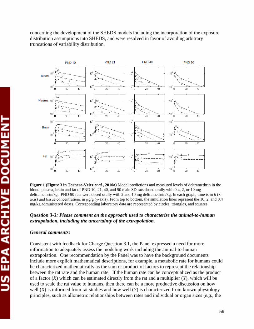
59

concerning the development of the SHEDS models including the incorporation of the exposure distribution assumptions into SHEDS, and were resolved in favor of avoiding arbitrary truncations of variability distribution.

Figure 1 (Figure 3 in Tornero-Velez et al., 2010a) Model predictions and measured levels of deltramethrin in the blood, plasma, brain and fat of PND 10, 21, 40, and 90 male SD rats dosed orally with 0.4, 2, or 10 mg deltramethrin/kg. PND 90 rats were dosed orally with 2 and 10 mg deltramethrin/kg. In each graph, time is in h (x-axis) and tissue concentrations in μg/g (y-axis). From top to bottom, the simulation lines represent the 10, 2, and 0.4 mg/kg administered doses. Corresponding laboratory data are represented by circles, triangles, and squares. Question 3-3: Please comment on the approach used to characterize the animal-to-human extrapolation, including the uncertainty of the extrapolation. General comments: Consistent with feedback for Charge Question 3.1, the Panel expressed a need for more information to adequately assess the modeling work including the animal-to-human extrapolation. One recommendation by the Panel was to have the background documents include more explicit mathematical descriptions, for example, a metabolic rate for humans could be characterized mathematically as the sum or product of factors to represent the relationship between the rat rate and the human rate. If the human rate can be conceptualized as the product of a factor (X) which can be estimated directly from the rat and a multiplier (Y), which will be used to scale the rat value to humans, then there can be a more productive discussion on how well (X) is informed from rat studies and how well (Y) is characterized from known physiology principles, such as allometric relationships between rates and individual or organ sizes (e.g., the

60

¾ power relationship). In addition, as noted in Charge Question 3.2, the Panel recommended that the Agency conduct a sensitivity analysis to determine which parameters in the model are drivers, and what additional empirical data are needed to fill gaps that have the greatest impacts on the model. The Panel recommended that the Agency apply methods to assess the gamma parameter used for the rat to human in vitro and in vivo extrapolations. A rigorous review of the published literature should identify biological properties relevant to the species differences, which could then assist EPA in filling some data gaps until empirical rat or human data (in vivo and in vitro) can be collected. These data could then be used to place bounds on the uncertainty by evaluating the distributions of the parameters used in the analysis. Specific comments: The Panel discussed several specific aspects of the animal-to-human extrapolations in the modeling.

1) Oral absorption. The Panel commented that there is a lack of information on how the oral absorption rate was extrapolated across species, as well as from in vitro to in vivo scenarios. These parameters may be important for estimating dose-metrics, but they will require careful consideration and data prior to inclusion in the PBPK model. See also the previous discussion in Charge Question 3.1 on the importance and limitation of the modeling with respect to oral absorption.

2) Tissue distribution-diffusion limitation (i.e., permeability-surface area coefficients). One particular area of uncertainty discussed by the Panel was how the diffusion limitation was included in the model with regard to human versus rat values for the permeability-surface area coefficients of the various tissues. In more traditional PBPK models transfers of the modeled toxicant to tissues are predicted assuming that full equilibrium is achieved between the tissue and the blood flowing through the tissue. In models assuming a diffusion limitation, the “permeability-surface area coefficient appears to be defined as the reduced fraction of the transfer expected under a perfusion model, which actually occurs (see also comments to Charge Question 3.1). One panelist pointed out that the current model assumes that all tissues are diffusion-limited, and there are some physiological conditions that could impact the distribution of a pyrethroid (or metabolites) into tissues in humans, which will not be captured by the values used to represent diffusion into the standard 70-kg male in the PBPK model. For example, the rates of obesity/diabetes in the American population are increasing, which would result in a different set of human of permeability-surface area coefficients than the typical values included in the model. The diseases would affect tissue surface area, the blood flow to each compartment and the relative tissue lipid percentiles. The Panel stated that these scenarios will not be modeled in a standard rat to human extrapolation. Another panelist explained that there is little basis for treating permeability-area coefficients from animals or humans differently, and recommended adopting the values estimated from the rodent data directly into the human model. As size increases, volumes

61

increase relative to surface areas. Therefore, diffusion parameters would be expected to decrease for humans relative to rodents. One might consider sensitivity analysis for a body weight (1/3) correction based on human/animal relative body weights. However, this difference may already be implicitly accounted for in the decrease of perfusion per unit tissue volumes, if the diffusion parameter is effectively a multiplicative modification of the transport expected from perfusion.

3) Lactational exposure. The Panel indicated that additional empirical data on lactational exposure in rodents should be collected. These data are necessary to determine the metabolic species of pyrethroid contained in the urine and feces of very young animals. This would also allow the role of Phase II enzymes (and de-glucuronidation in the gastrointestinal tract to be better understood in young animals. This is critical, since the parent substance (e.g., permethrin, deltamethrin) is understood to be the toxic species. Currently there is a lack of knowledge concerning enterohepatic recirculation in young animals.

4) Low tissue concentrations below the Km. The Panel also raised a concern with the assumption of low tissue concentrations of pyrethroids, particularly at concentrations that are below the Km of the metabolic enzymes in all tissues, e.g., in the placenta of a pregnant woman and in a young child (i.e., nursing or post weaning). In addition, the Panel noted that literature support was not provided for this assumption. Information supporting this assumption should be clearly demonstrated so that the model is defensible.

5) Piperonyl butoxide impact. As mentioned in the response to Charge Question 3.1, many

pyrethroid formulations contain piperonyl butoxide or other Phase I enzyme inhibitors. The inhibitors are included in the formulation to increase the pesticides’ efficacy in the insect by slowing down the breakdown of the pesticide. The Panel commented that if piperonyl butoxide is able to inhibit or modify the human enzyme systems, then it is plausible that the rates and amounts of parent and metabolites would be different than in the case of neat compound alone.

Question 3-4: Please comment on the plausibility and limitations of model-predicted dose-metrics, such as area under the curve (AUC), peak tissue values, time above a toxicological threshold, or AUC above a toxicological threshold, in analyzing animal dose-response data and in extrapolation to humans.

Panel Response

The Panel recommended flexibility in the model structure and in the dose-metric chosen. A carefully calibrated and validated pyrethroid PBPK model could be used to estimate any of the proposed dose-metrics. The Panel considered the array of dose-metric options listed by the Agency and expressed preference for either “simple peak concentrations” or “AUC” as dose-metrics. T here was not enough information about the mode(s) of action of pyrethroids to postulate specific a “toxicological threshold” or “the time over the threshold” values. The “correct” dose-metric is dependent on the pharmacodynamics. Therefore, multiple dose-metrics

62

are recommended for studying extrapolation of data from animals to humans. The Panel stated that it was not sufficient to rely on a small set of dose-metrics for cross-species extrapolation until an integrated pharmacokinetic/pharmacodynamic model has been developed. The model should be constructed to be flexible enough to incorporate a wide array of potential dose-metrics and should retain the ability to generate time-dependent variation. As pointed out by one Panel member, the endpoints will determine the correct dose-metric. Before any specific dose-metric (or set of dose-metrics) can be chosen, the Panel indicated that the limitations in the PBPK model outlined in Charge Question 3.1 will need to be addressed, including the effects of age, diseases such as obesity and diabetes, gender, pregnancy and body weight. Use of the 70-kg male human may not be appropriate to assess internal exposure to pyrethroid pesticides across the population. Many Panel members considered the AUC to be the most robust dose-metric among the options because AUC integrates all the events that occur during the time period of the PBPK simulation. In addition, AUC has been used widely as the closest estimate for the effective internal dose for a variety of applications, such as in pharmaceutical research. In terms of a pyrethroid-specific application, the Panel considered AUC to be the most plausibly useful single dose-metric. While there are several proposed target sites of action for pyrethroids, e.g., sodium channel and calcium channel disruption, the AUC would provide a measure of exposure (and hence, disruption) of all of them. Whole animal toxicity (measured as secondary lesions) depends on the number of target sites disrupted, and the time for which disruption is maintained. If this is the endpoint of interest, then AUC would also be a useful dose-metric. The Panel recommended using a time-dose-response data set to evaluate the relationship between the AUC and time of onset of symptoms in the rat. The use of “peak tissue value” was discussed as a potential dose-metric; however, the Panel thought it would likely underestimate the true overall dosage under those circumstances when there are multiple high tissue values associated with the simulated exposure scenarios. This situation would be rather common in the simulation of pesticide exposure that occurs in daily sporadic events. Also, the “peak” tissue value would still need to be integrated in order to take into account the “time” component (which defines the shape of the peak, and under these conditions this exercise is similar to the AUC, but takes into account only part of the data. One panelist was unconvinced that the data supported the use of brain concentrations of parent compound or metabolite(s) as the correct metric. This conclusion is based on the influence of the chemical on non-CNS structures. Evidence is accumulating in the literature that identifies the interaction of chemicals with targets in which effects on endocrine systems appear to be critical for low dose effects (and for which non-linear dose-response curves are relevant). For example, Prater et al. (2002) demonstrated the effects of permethrin on the thymus in a relevant dose-range. By using the AUC and peak levels of parent pyrethroids, this information can be used to inform further iterations of this PBPK model. Question 3-5: The presentation described methods for addressing uncertainty in model parameters and extrapolation from animals to humans. What other important sources of uncertainty need to be addressed for either the SHEDS exposure model or the PBPK model?

63

The Panel outlined several areas of uncertainty in the data used for model development, e.g., the influence of censored data on parameter estimates, pharmacodynamic differences among species and individuals, and techniques for addressing individual uncertainty and distributions in various age groups. In addition, the Panel pointed out that there is also uncertainty in the “form of the model” that should be considered. As new information becomes available some of the PBPK model compartments might need to be expanded. This may be particularly important as the generic model grows in utility to accommodate more chemicals or the need to incorporate more complexity in specific compartments. The approach for uncertainty analysis currently involves the aggregation of results from SHEDS-Residential (or SHEDS-Dietary) for each individual, and using them as inputs and parameters for doing PBPK simulation. The Panel indicated that of the various sources of uncertainty currently not addressed by the SHEDS and the PBPK model, the two major types are:

1) Uncertainty due to a limited number of samples. Specifically, the tails of the distributions may not be adequately captured by a small number of uncertainty samples (typically of the order of 100 used in the SHEDS simulations). The sampling approach used in SHEDS involves sampling along a large number of dimensions (with each dimension corresponding to one independent random variable). The number of points to adequately sample from a high-dimensional space increases exponentially because the corresponding sampling space becomes “vastly empty” as the dimensions increase (Tarantola, 2005).

2) Model/structural uncertainties. These uncertainties will occur when multiple alternative formulations are available. One approach to reduce this uncertainty involves the application of Bayesian model selection and model averaging techniques (Toni and Stumpf, 2010).

The approach for uncertainty analysis currently involves the aggregation of results from SHEDS-residential for each individual, and using them as inputs and parameters for doing PBPK simulation. All the uncertainty parameters are sampled during the SHEDS simulation and passed on to the PBPK model. This means that two samples that share the same exposure parameters probably will have different PBPK model parameters. This process involves repeat simulations. A nested approach (Xue et al., 2006) has been used with SHEDS to characterize uncertainty and variability separately. This same approach can be used to characterize separately the uncertainty and variability due to PBPK model parameters and due to SHEDS exposure model parameters. Using the nested approach to uncertainty analysis can result in substantial computational efficiencies by simply fine-tuning the sampling process. Currently, outputs of uncertainty analyses are further analyzed by linear regressions to identify important parameters. However, other tools and approaches for computationally efficient sensitivity analyses and for identifying contributions of individual parameters to overall uncertainty are widely available (e.g., Saltelli, 2008). The Panel recommended that other approaches be employed in addition to the simple regression approach currently used by EPA. One Panel member stated that it was not clear whether human variability in pharmacokinetics was incorporated within the PBPK portion of the model as it was within the exposure portion of the model. There is considerable earlier literature on uncertainty in pharmacokinetic parameters (e.g., see Hattis and Lynch, 2007). There was some mention in the background material of

64

truncation of the variability parameters at two or three standard deviations. One panelist noted that it was generally inadvisable to do so because of the possibility of neglecting extreme percentiles of the real distribution of exposures, giving rise to understatement of the real likelihood of extreme values of resulting internal dose distributions consistent with possible toxicity. One additional area of uncertainty was with the use of the urinary markers, e.g., DCCA. One Panel member explained that this urinary metric is a useful metric for comparison with SHEDS output, but not for total body load. The half-life of permethrin is biphasic – urine can be used if collected over the course of days, but spot urine or 1/day urine samples will necessarily miss some of the body load. Excretion studies in Table 2 of the Agency’s background document on PBPK models of pyrethroids (Tornero-Velez et al., 2010a) identify the excretion patterns from dermal exposure as under-represented in the urine (% dose). Therefore, there is a need to consider non-first pass mechanisms and non-urinary excretion. As a consequence, the Panel indicated that urine is not a good metric for total body load. Issue 4: Model Evaluation BACKGROUND: Model evaluation is an important component of model development that helps ensure that the quality of the model meets the regulatory needs of OPP and other end-users. In performing its model evaluation, the Agency compared SHEDS model output – specifically exposure and urinary concentration estimates – with both output from other exposure assessment models and data from observational studies. These comparisons permit the SHEDS development team and model end-users to compare and contrast outputs among different models, to compare estimates with measured real-world data, to explore and investigate reasons for any differences, and to evaluate and better understand the reasons behind these differences. As part of the model evaluation procedure for SHEDS, the Agency has attempted to evaluate the SHEDS model in a number of ways. These include:

1) comparison of SHEDS-Dietary cross-sectional output to DEEM-FCIDTM; the DEEM-FCIDTM model is commonly used by OPP in its regulatory decisions and was reviewed by the SAP in 2007 (see SHEDS-Dietary Technical Manual (Section.2.8.1) and EPA 2010 Response to Comment (p.10)).

2) comparison of (a) SHEDS-Dietary arsenic and permethrin estimates against duplicate diet data and (b) the predicted urinary concentrations from the SHEDPBPK linked model with the measured arsenic concentrations in urine from the 2003-2004 NHANES biomonitoring program (see SHEDS-Dietary Technical Manual and link to Xue et al. 2010 article provided in background materials).

3) comparison of SHEDS-Residential outputs with outputs from other models or calculation methods (ORD’s Draft Protocol, OPP’s Residential Standard Operating Procedures (1997), Calendex, CARES, and ConsExpo) which was originally organized as a day-long symposium at the annual meeting of ISEA in 2008 held in Pasadena, CA (see slides in background materials).

65

4) following the model quality assurance procedures as detailed in Chapter 8 of the SHEDS-Residential Technical Manual and EPA’s SHEDS-Multimedia Quality Assurance Project Plan (QAPP) these included EPA-contractor cross-checking of the code and hand-calculation verification on a subset of data for a simulated individual to ensure the SHEDS-Residential algorithms were implemented and performing as intended.

Question 4: Please comment on the process used to evaluate SHEDS. Are the above listed ways in which SHEDS was evaluated appropriate? In what ways could they be improved? Are there other methods through which the model should or can be evaluated? Are there other data (e.g., biomonitoring data, duplicate diet data) that the Panel is aware of through which the SHEDS model can be compared?

General comments:

Panel Response

The Panel agreed that linking a probabilistic exposure model (SHEDS) with a PBPK model provides a unifying approach that will potentially furnish a way of assessing new compounds of concern or combinations of compounds. Ideally, the performance of SHEDS in the simulation of exposures should be evaluated against sound external data and modelling that can provide a gold-standard benchmark; however, in the opinion of the Panel, such a gold-standard is not currently available. Rather than focussing on whether the approaches are appropriate or not, the Agency should use this opportunity to examine the results from the evaluation to examine in detail where discrepancies and agreement exist. Further analyses would provide greater clarity in the understanding of the outcomes of the various comparisons. The Panel encouraged the Agency to continue their ongoing efforts to evaluate the model system, and to define the reliability of the model.

In general, the PBPK model comparisons described by the Agency provided useful information on the application of the full model. In the case of permethrin, the Agency concluded that the model evaluation provided confidence in the SHEDS-Dietary model. However, in some areas, there is a lack of similarity between the model prediction and the measured data, and these disparities should be examined in detail.

Specific comments:

1) General principles of model evaluation In general, model evaluation of a complex system such as SHEDS linked with a PBPK model is difficult, but necessary. The Panel stated that model evaluation is a five-part process that attempts to answer a number of important questions. The Panel went through the following stages in its discussion of the Charge Question:

a) Quality Assurance: Provides a check on the extent to which the model, as implemented in code, reflects the conceptual model. The Panel agreed that the SHEDS-Multimedia Quality Assurance Project Plan (QAPP) being used appears to be sound and emphasized that it is of the utmost importance that all steps of the QAPP be followed rigorously in all phases of model development and coding.

66

b) Calibration: Provides a check on how well the model reflects the trends or relationships that are known empirically or theoretically, and that the model predictions are reasonable. The check examines the overall model fits, e.g., R-square statistics, observed-predicted plots, and prior-posterior distribution comparisons (Q-Q plots) for key model parameters.

c) Validation: Usually carried out in two parts: 1) comparison of predictions with those of other similar models (benchmarking) [performed by EPA] and 2) prediction of data not used in model development or calibration. The Panel recommended the latter to the Agency. [Note: no information on the latter process was available to the Panel.]

d) Sensitivity analysis: Identifies the model parameters or components that are particularly important in determining model outputs, and assesses the reasonableness of the measured sensitivities.

e) Extrapolation: Used to assess how well the model works when translated to another scenario or chemical, how well it handles extreme scenarios, and how well it works for acute versus chronic exposures.

2) Checking the code and algorithms

The Panel stated that checking the code and functionality by hand, as specified in the QAPP, is a major undertaking but worthwhile, since hand calculation is an excellent way of checking the structure of the SHEDS model and assuring that the conceptual model is truly replicated. This is especially applicable when there are many factors, possibly interacting, that significantly affect the model’s outcome. This part of the evaluation process is easier to carry out than checking the validity of the assumptions, model structure, and results. The latter is necessary, but difficult to achieve, in part, because of the lack-of-fit when benchmarking the model.

The Panel found the algorithms in the SHEDS model are relatively straightforward, use simple algebraic calculations that involve random samples, summations over multiple time steps, and a large number of virtual individuals. Therefore, diagnostic analysis of the model, focusing on the impact of variations in different inputs on model outputs is an appropriate approach. The comparative evaluation of SHEDS has focused so far on relative estimates of population variability without presenting the impact of the underlying uncertainty. A comparison of the cumulative frequency distributions of different models along with the corresponding “uncertainty clouds” would provide more insight into the results of individual models. A global sensitivity and uncertainty analysis with a large number of model simulations (of the order of 1000 uncertainty runs with 1000 individuals that focus on a small number of simulation days) would help to identify the inputs and parameters that have the most impact on outputs. In general, comparisons among distributions should be made with both tabular presentations of the comparative percentiles of the distributions, and probability plotting methods. This point was illustrated by one Panel member who used the assessment of the results of the SHEDS-PBPK permethrin case study discussed in Issue 5. The current comparative plots of cumulative distributions are generally uninformative and it was recommended that they should not be used in the future. Generally there is a need for enhanced visualization of model outputs, especially when studying the tails of the distributions predicted by a single simulation or when comparing multiple model simulations. For any future SAP meetings, the Panel recommended that EPA

67

provide the Panel members with the full model outputs of a comprehensive sensitivity/uncertainty simulation, then interested Panel members could explore the model outputs with visualization tools without having to run time-consuming simulations.

3) Model robustness and evaluation: Comparison of SHEDS to CARES, Calendex, ConsExpo

In general, the model comparisons described in the Agency’s background materials and presented at the SAP meeting provided useful information on the application of the full model. In the case of permethrin, the Agency concluded that the model evaluation provided confidence in the SHEDS-dietary model. However, in some areas there was a lack of similarity between the model prediction and the measured data; these differences should be examined in detail. Greater clarity in the understanding of the outcomes of the various comparisons may be gained from further analysis. The SHEDS Dietary Model Technical Manual presents an example highlighting the negligible impact of outliers on the 99.9th percentile. This robustness can be misleading. Two factors have the potential to produce this result: 1) the insufficient sampling of a particular entry and 2) the compensation of errors in one dimension by similar factors in another dimension in a large pool of samples.

To date, the Agency has spent a lot of effort comparing SHEDS to other models whose validity may not have been so closely checked, and thus, may not be good benchmarks, and certainly not gold standards. The SHEDS model has been evaluated by comparison of the variability distribution of the model with that of other probabilistic exposure models such as CARES, Calendex and ConsExpo, but agreement among some of these models is not a strong basis for judging whether SHEDS model performance is satisfactory. That is, similar results among models do not equate to increased confidence in the appropriateness of the assumptions used in the model. When models based on similar assumptions produce similar results then this provides some level of confidence in the functioning of the model at the level of input, coding, and internal connections. Since most of the models used in the Agency’s comparisons use similar probabilistic algorithms and have a large input data requirement (including pesticide use profiles and demographic information) agreement among these models is mathematically necessary, but not a sufficient condition for acceptance of the robustness of the model. They could all be equally right or wrong. One Panel member noted that the simpler models predating SHEDS tended to make conservative assumptions whenever simplifying assumptions were needed. Therefore, it is not surprising that a more refined model like SHEDS can lead to less conservative conclusions such as lower values for upper percentiles, as was observed in many of the ISEA symposium presentation examples.

An additional evaluation step for model performance is the comparison of combined distributions of uncertainty and variability (i.e., adding uncertainty clouds around the currently shown variability distributions in, for example, Slides #6 and #7 of EPA's Presentation on SHEDS-Multimedia Model Evaluation Efforts, see Regulations.gov, OPP Docket: EPA-HQ-OPP-2010-0383). This additional comparison will provide insight into how much uncertainty is present in the estimates of each model.

The Panel expressed some reservations concerning the quality of some of the published data sets (see examples provided below). One potential problem with complex multi-parameter models is that if there are correlations between parameters or sets of parameters, then changes in one

68

parameter can be matched by equivalent shifts in the values of other parameters, and the same output can be achieved with different sets of parameter values. A small deviation between models could be due to large differences in the relative values of sets of parameters between models. For instance, although total daily exposure in a 365-day time series is similar for CARES and SHEDS, the proportions attributed to dermal and oral routes are markedly different between the two models. Therefore, the Panel stated it would be worthwhile to examine in detail the extent to which the various models agree or disagree, rather than just looking at the final outcomes. [Note: Some of these comparisons have already been done and presented to the SAP for its review and comment.]

The Panel stated that a gold-standard benchmark for the evaluation of the performance of SHEDS against sound external data and modelling is not currently available. Rather than focussing on whether the approaches are appropriate or not, the Panel suggested that the Agency examine the results from the evaluation to examine in detail where discrepancies and agreement exist. For instance, comparisons of permethrin residues between SHEDS and duplicate food samples collected in the Children’s Total Exposure to Persistent Pesticides and Other Persistent Organic Pollutants study (CTEPP) reveal some differences. A notable example is in the comparison of the 50th and 99th percentile cis/trans ratios of permethrin in SHEDS with measured data. The Agency concluded that there was a good match between isomer ratios of mean measurements. However, the permethrin data generated by CTEPP do not seem to be consistent with the usually observed cis/trans isomer ratio (1:2 to 2:3) of permethrin. Although the upper percentile predictions appeared to “match well” with the CTEPP data, the comparison at the 50th percentile did not show close similarity. This could be due to important differences between the ways in which samples (such as liquid versus solid) and data from samples below the level of detection were handled in the two studies. The Agency speculated that in this case the lack of agreement was most likely to be due to the use of zero residue level for samples that fell below the level of detection in the CTEPP database. While this may be the case, this explanation should be further explored and substantiated with additional model runs, since comparisons of central tendencies are pertinent to model evaluation. Comparisons between SHEDS and CTEPP would benefit from a more in depth analysis. The Panel recommended that the Agency should critically review the CTEPP data before using it to inform the future development of the SHEDS-PBPK model.

Another illustration of discrepancies among models is the comparison that was made between the relative contributions of various commodities to dietary exposure within SHEDS with the contributions based on either CSFII or NHANES consumption data. There was poor agreement between the contributions of the two most important commodities, spinach and lettuce, in the two model predictions. Assuming that the total exposure estimated from these two consumption databases are similar, it would be helpful to know what factors might have contributed to the substantial difference in the percentage of contribution by the two top-contributing commodities. Furthermore, since it is not entirely obvious that 3-5 year-old children are generally high eaters of spinach and lettuce; it would be helpful to provide the context for these high-end exposures by providing the levels of consumption for these commodities. Since exposure is a product of consumption and residue level, it may well be reasonable that these high-end exposures are due to a combination of a high level of consumption (e.g., children of vegetarian families) and high residue. The Panel noted that it would have been helpful in the examination of the data to have the total exposure tabulated at various percentiles in addition to the graphical presentation.

69

Another area where caution should be exercised is the combination of survey data from multiple years for use as model input. Factors may be operating that substantially reduce the resolution of model predictions and comparisons, and these should be further investigated. For example, the yearly residue data distribution may not be random, but rather reflective of factors such as pest infestation patterns, or trends in patterns of food consumption. Changes in food consumption data (e.g., CSFII versus NHANES) can provide realistic representations of changes in dietary behavior over time. A more careful study of patterns inherent in the various databases could provide greater clarity in comparison exercises. Evaluations which use only the NHANES data are not sufficient, since these data provide but a snapshot at a large, general population level. Since the SHEDS model is intended for application in regulatory settings, it should be robust and accurate for subpopulations of highly exposed individuals.

4) Field Data

The Panel stated that sound field data (not used in the development of the SHEDS-PBPK model) were needed to test the model and to identify areas of strength and weakness. The addition of biomarker production was a key recommendation of the August 2007 SAP (SAP, 2007). The Panel commended EPA for implementing this recommendation through the introduction of a scheme to predict biomarkers. The feasibility of model evaluation has been greatly enhanced by this addition. The Panel commented that the biomonitoring data should be of the same quality as those collected in the National Agricultural Workers Survey (NAWS) study. It may be necessary to obtain the data may need to be obtained from designed studies that could be linked with the development of biomonitoring equivalents (Hays et al., in press; Hays et al., 2009; Hays et al., 2008).

5) Use Published Data

The Panel commented that there were many pharmacokinetic and biomonitoring data sets that cover a range of exposure scenarios, and that are available in the literature (e.g., Berger-Preiss et al., 2009). The Panel suggested that it would be worthwhile to review these published data to examine the changes in biomarkers that occur for particular known-dose exposure scenarios, even if they do not match exactly the exposure scenarios in SHEDS. These sources of information may provide checks on the outcomes of the PBPK model for particular measured exposures. Several examples were provided by the Panel.

a) A number of studies (Fortin et al., 2008; Naeher et al., 2008, 2009), albeit with small numbers of subjects [e.g., 120 adults, 120 children (aged 6 to 12 years) in the Fortin study] provide an indication of the potential impact of factors such as the use of pyrethroids in the treatment of head louse infestations. This can lead to extreme exposures (and matching high levels of urinary biomarkers) that may cause some deviations from the levels predicted by the SHEDS model.

b) Studies (e.g., Appela, et al., 2008) on the exposure to pyrethroid-impregnated uniforms provide useful pharmacokinetic and biomonitoring data that could be used to assess the dermal absorption part of the PBPK model.

c) Data from the longitudinal Children’s Pesticide Exposure Study (CPES) could be used by the Agency to further evaluate SHEDS, particularly for the dietary component (Lu et al., 2006a-b, 2008, 2009). CPES collected multiple consecutive daily dietary

70

consumption information for a 12-month period (separated by seasons) from a group of 46 children ages 3-11 living in two different geographical locations. Along with the consumption data, CPES also analyzed selected organophosphates, pyrethroids, and metabolites in daily urine samples.

d) The Metro Atlanta Cohort (MAC) study (Riederer et al., 2010), similar to CPES, could also be used by the Agency for the same objective. The MAC study enrolled participants ages 12-65 who lived in three counties in the metropolitan Atlanta area and used a random statistical sampling method based on the 2000 Census data for the three counties. MAC collected 6 daily urine samples in each of the 12 months, as well as the daily dietary consumption information. Both MAC and CPES studies also measured pesticide residues in the 24-hour duplicate food samples of the participants once during the study period. Most of the CPES data have been published in peer-review journals, and are (or will be) available to the Agency.

e) Good quality, comprehensive data sets are available from earlier studies for some compounds (e.g., chlorpyrifos) with reliable biomonitoring data (Barr and Angerer, 2006; Timchalk et al., 2002; Timchalk and Poet, 2008). These could be used to measure the reliability of specific components of the PBPK model.

The Panel issued a note of caution. Do not modify or re-calibrate SHEDS on the basis of a lack of agreement between predicted outcomes and published data without a thorough examination of the quality of the published data. For instance, the Agency applied an adjustment factor in order to reduce the difference between SHEDS predicted TCP levels in urine and the measured levels in the Jacksonville study (Naeher et al., 2010). In the opinion of some Panel members this was neither necessary nor advisable.

6) Suggestions of other ways in which the model could be evaluated

The Panel suggested some other ways in which the model could be evaluated, and commented upon ways in which the presentation of the data could be improved to facilitate the interpretation and evaluation of the model output. There were several suggestions for ways in which to test the general reliability of the model inputs. Diagnostic model evaluation could be achieved by comparing the input values sampled by the model with corresponding distributions of the input variables. Comparison of full model outputs with simple predictions based on, for instance, total pesticide production/application and average consumption patterns, could also be helpful. Given the stochastic nature of the draws that are made in the SHEDS model, it should be possible to estimate the number of specific meals that are consumed in the U.S. in a year. These national estimates could be compared with the consumptions of commodities predicted by the SHEDS simulation for specific proportions of meals or commodities. The Panel suggested that it may also be useful to compare overall exposure through residues with records of pesticide usage. The approaches outlined in this paragraph would provide quantitative measures of the value of additional information available in the risk assessment.

Another approach to testing the SHEDS model would be to create a large artificial data set for which the statistical structure and model outcome are known, and use this to test the model. This could also be applied to the simulation of exposure, where the use of a diagnostic data set with known distributions, and seeded with some artificial extreme values for both dietary and dermal

71

routes would provide useful checks. This could be achieved by adding one or two entries (e.g., dietary records or food products containing a large amount of contaminants of concern) and studying how frequently the uncertainty and variability propagation is able to capture these records accurately. Failure to capture them would indicate the false robustness. This approach would also enable an examination of defined areas of the total data space. Additional analysis of the tails of the distribution is needed because the model simulations appear to produce very long tails compared with available biomonitoring data. In this general context, it would be useful to assess the ability of SHEDS, which is geared to modelling chronic exposure, to deal with acute exposure scenarios. Exposure data from the latter would facilitate testing of the PBPK model since other pharmacokinetic models designed to model acute exposures are available to provide comparisons.

Issue 5: SHEDS-PBPK Permethrin Case Study

Question 5-1: EPA has used a pyrethroid insecticide, permethrin, as a case study to link the SHEDS exposure model with PBPK modeling in order to be able to better interpret and understand exposure data in terms of dose and target-organ dose and assist in refining exposure estimates and associated risk. Please comment on the approaches and offer alternatives and suggestions for:

1) linking dietary consumption diaries and residential activity information (e.g., key factors used for matching food consumption and activity pattern diaries such as caloric consumption);

2) quantification of dietary vs. residential contribution, including relative contribution of residential exposure pathways (dermal, inhalation, hand-to-mouth, object-to mouth);

3) D[iversity] and A[utocorrelation][D & A] longitudinal diary assembly approach (Glen et al., 2007, reviewed for residential module by 2007 SAP);

4) identifying significant contributors at upper percentiles of dietary exposure; and 5) techniques and utility of bootstrapping approaches for quantifying uncertainty and its

interpretation.

Panel Response

General comments: The Panel agreed that the permethrin case study to link the SHEDS exposure model with PBPK modeling was useful and indicated an overall correspondence of predicted and observed biomarker values that were better than could usually be expected (see the discussion in the response to Charge Question 5-2 below).

The Panel concluded that the overall accuracy of the SHEDS/PBPK predictions for high percentiles seemed to be good when compared with existing lab and survey-based databases; however, further research is needed where the agreement between model predictions and empirical data was not as good. For rats (Figure 3, Tornero-Velez et al., 2010a), the agreement among predicted peak tissue concentrations was very good (generally within about a factor of two), while the agreement among 48-hour brain levels was not (often under-predicting by about a factor of 10). The Panel indicated that an investigation of whether the weaker match at longer

72

times is important depends on how the modeled data will be used by EPA. The mean and upper percentiles of the urinary excretion predicted for humans shown in Figures 10-11 of the Agency background document (Tornero-Velez et al., 2010a) generally match NHANES data within even less than a factor of two. The Panel commented that many of the results presented by the Agency of multiple exploratory approaches to assess the validity and robustness of this model were illuminating; however, the variations in the assumptions or modifications made to accommodate these approaches (e.g., the handling of dietary residues less than the LOD, skin loading and absorption, and the amount and permeability of clothing) can give the impression of an ad hoc process used to inform the modeling. The Panel indicated that the Agency should strive to rationalize the differences among the various test conditions and assumptions to make them more uniform (or thoughtfully assess the impact of unavoidable differences).

Specific comments:

1) Linking dietary consumption diaries and residential activity information

The Panel supported the Agency’s basic approach to use caloric consumption as a link between dietary and residential exposures is reasonable. However, the degree to which a simulated individual was actually linked to both the dietary and residential components of SHEDS and between SHEDS and PBPK within the various studies presented to the Panel was not completely clear. The Agency stated that such linkages are “not a standard component or feature of SHEDS at this time.” Clearly the gender and age of individuals were linked both within SHEDS and on to PBPK. The Panel encouraged the Agency to incorporate linking caloric consumption as a correlate for metabolic activity as a standard feature of future versions of these models. With or without that linkage, the degree and direction of cross-correlation between activity, exposure, and metabolism needs to be explored further; in particular, the influence of cross-correlations on the validity of the two-stage Monte Carlo simulations that are currently being run needs to be explored. If exposures are positively correlated with metabolism, then the two independently run simulations (first via SHEDS, then via PBPK) will over-estimate the variability that would result from one properly linked simulation; alternatively, negative correlations will under-estimate the variability from a properly linked simulation.

2) Quantification of dietary vs. residential contribution The Panel agreed that it was reasonable for the Agency to use SHEDS to explore relative contributions to exposure, but that more validation of this issue is needed. While the ability to use such approaches is another unique aspect of the SHEDS-PBPK model, concerns about these contributions were a frequent topic during discussion of other Charge Questions to this Panel. Specifically, concerns are described within this report in regard to the role of drinking water and breast feeding of infants (specific comment #2 to Charge Question 2-1, limitation #3 to Charge Question 3-1, and specific response #3 to Charge Question 3-3), to the role of seasonality and climate (specific comment #3 to Charge Question 2-1), to the variability in oral absorption (specific comment #1 in response to Charge Question 3-3), and to the modeling of clothing and skin loading (specific comment #2 to Charge Question 2-1, limitation #8 to Charge Question 2-2, and specific comment #2 to Charge Question 3-3). The Panel recommended that in the future that the Agency should evaluate the proportion of exposure attributed to intake through the diet, and residential environmental exposure through the use of other datasets, such as NHANES,

73

CPES, and MAC (as described in Panel’s response to Charge Question 4). Clearly the predicted relative contributions of particular exposure pathways are dependent upon model assumptions and may not be straightforward reflections of input data. As noted above, several panelists questioned the accuracy of some modeled exposure processes that could affect the relative contribution of some routes of exposure. For instance, dermal exposures are likely to be underestimated (see discussion of technical merits under Charge Question 2.2 and in Tomalik-Schartei (2005) and Kissel (2010). If the description of dermal absorption is improved, then the relative contributions of the various routes of exposure will shift. In addition, dermal exposures from lice shampoos (see Naeher et al., 2009) and the potential for exposure via permethrin-impregnated clothing should also be considered (see Rossbach et al., 2010 and U.S. Army data regarding these exposures in Army personal). While pyrethroids are relatively non-volatile, pyrethroid residues do adhere to dust particles and have a longer indoor environmental half life; thus, resuspended dust particles (e.g., after dusting, vacuuming) should be considered as a component of inhalation exposure. In the process, data specific to certain carpet types (e.g., wool versus polymer-based) should also be considered (see Butte and Heinzow, 2002) and Bradman and Whyatt, 2005). Finally cross-pathway comparisons should be made on a consistent basis (i.e., absorbed dose vs. absorbed dose, not potential dose – see response to Charge Question 2-2).

3) D[iversity] and A[utocorrelation] [D & A ]longitudinal diary assembly approach: The Panel concluded that the use of D & A approach is reasonable for assembling the longitudinal diary for food consumption in light of the practical difficulties of collecting longitudinal data. However, this approach has its shortcomings (as described below). In addition to the steps suggested below, the Panel recommended that the Agency seek additional data to further refine the estimations of the D & A values as the current D & A values were estimated from a single small study. The simulated distribution should be able to mimic the true patterns in the population. However, because the D & A approach samples and combines a large number of diaries for each individual (at least in the eight (8)-diary sampling approach), its simulated result will have less overall variability than the original diaries but will also lead to a particularly rapid decrease in rare diets. Mathematically, the prevalence of each unique diet [P] will decrease when it is combined in a group of some number [N] of diets to i. While the prevalence of vegetarians in the U.S. population is not known precisely, a 2003 Harris poll indicates it might comprise about 3% of the population. If vegetarians also comprise 3% of the sampled diaries used by SHEDS, a vegetarian diet will comprise only 0.032 = 0.09% of two such diets combined at random (or only one out of one thousand simulated persons) and 7x10-13 of eight such diets (would virtually never be a part of an 8-diet simulation). As a result, other high-end ("ever eat") and low-end ("never eat") exposure scenarios will also not be captured adequately (e.g., vegetarians who consume large amounts of spinach that contain pesticide residues or people that never eat some types of foods that often contain pesticide residues). The effect of the size [N] of such combined samples and of autocorrelation on this outcome should be investigated.

74

Now this effect might be particularly important for some dose-metrics and not for others; however, the more critical scenarios have not been explored and those metrics are not defined. One option to avoid this problem is to use an approach based on a combination of multiple sampling options in order to characterize the population variability adequately. These options can include some sets of individuals whose dietary information is sampled based on a one- and 8-diary repetition (to capture the tails of the exposure distributions) as well as a large set of individuals whose dietary information is sampled by the D & A approach (which will allow for more “intra-individual variability”). Another option is to utilize food preference (food frequency) survey data that describes population fractions that eat certain commodities or groups of products, e.g., Tooze et al. (2006). Combining some form of Bayesian estimation that incorporates food frequency information with limited food diary information could create simulated diary patterns that replicate broader population trends. The food frequency information might, for example be used to inform correlations in the assembly of longitudinal diaries, ensuring that enough patterns of vegetarian diaries are combined to match the sample fraction of vegetarian diets to the population estimates.

4) Identifying significant contributors at upper percentiles of dietary exposure Many Panel members agreed that identification of upper percentile contributors to exposure is a very useful tool for assessing risk, especially for multiple routes and multiple chemicals analysis. An example is provided by the SHEDS-Dietary model’s prediction that children less than one year of age have the highest dietary exposure from spinach, lettuce, and cabbage. On the other hand, it is possible that the random sampling approaches will result in scenarios where some high-end exposure scenarios may not be captured adequately (e.g., vegetarians consuming large amounts of spinach that contains pesticide residue, as discussed in Charge Question 5-1b). In order to capture special subpopulations (e.g., high fish eaters, vegetarians), the algorithms should potentially use only one or two diaries, especially because it is unlikely that one can find multiple records matching both the age group and special eating profiles (even in the case of 8-diary aggregations). Moreover (as discussed in response to question 5-2 below), the simulations more often than not produce a more varied distribution than is observed in the reference database. A better understanding of the cause of this discrepancy would increase the confidence of some Panelists in the ability of this model to adequately characterize upper percentiles in other pesticide exposure scenarios. Another important tool for characterizing the high end of exposure from commodities that have a relatively small number of high end eaters is the “eaters-only report” shown in Table 2-6 of SHEDS-dietary Technical Manual. This eater-only exposure distribution is especially useful to ensure that these exposures are captured and retained separately, instead of being lost through shifting to the far right of a much larger sample distribution for the entire population that have many low contributors from other commodities also containing the pesticide of interest. Permethrin exposures through the diet are generally believed to be primarily chronic but exposures via residential applications or for use on head lice are primarily intermittent, acute

75

exposures. Thus, one additional issue to be explored is the different effects on the outcome caused by changes in short term versus changes in long-term exposures. In other words, how well is SHEDS equipped to handle exposure spikes?

5) Techniques and utility of bootstrapping approaches The Panel agreed that the bootstrapping approach is important to illuminate the influence of assumptions on the outcomes of the model and is useful for identifying simple metrics of the underlying distributions (e.g., the sample mean). However, the interpretations should not be generalized, especially when a relatively small number of model simulations is considered. In general, bootstrapping approaches should utilize as many samples as feasible; otherwise, minor inconsistencies may occur. For example, Table 2-7 of the SHEDS Dietary Technical Manual shows some irregular variations in the metric of concern (ratio of 97.5th to 2.5th percentile); whereas, in principle, a monotonic behavior of the data is expected across each row and each column. One area that deserves more investigation is the influence of the number of diaries chosen to characterize each simulated person (as discussed in Charge Question 5-1b). The bootstrapping approach is also important to risk assessment because the upper percentiles of dietary exposure are often the values of interest. At least one panelist expressed some reservation on how the outcomes of bootstrapping would adequately address the uncertainty issue at the upper percentile values when the majority of dietary residue values used in the bootstrapping process are very low, or non-detectable. Under this circumstance, the bootstrapping outcome may over-estimate the uncertainty at the upper percentiles. Question 5-2: Please comment on whether the model evaluation approach comparing the linked SHEDS-PBPK dose predictions and NHANES (National Health and Nutrition Exams Survey) biomonitoring data is reasonable. Are there other model evaluation methods that the Panel would like to see the Agency perform? The Panel concluded that the comparison between SHEDS-PBPK dose predictions and NHANES biomonitoring data is reasonable, but pointed out numerous caveats based on limitations and nuances within the existing databases (especially, but not exclusively, for NHANES) that make them less than a “gold standard.” Some obvious limitations are the impact of censoring that prevents the accurate prediction of dietary 50th percentiles and the fact that the censoring cut-points are not a constant across groups. Less obvious limitations include the sampling schedule, choice of biomarkers of exposure, artifact contamination, preformed metabolites in the environment, and short half-lives of pyrethroids. The Panel recommended that the raw data from NHANES be used rather than the Center for Disease Control’s (CDC’s) Report on Human Exposure to Environmental Chemicals (www.cdc.gov/exposurereport) because the summary data have several limitations. For example, when varying levels of detection (LODs) exist, the percentile estimates given in the summary data must be lower than the highest single limit of detection (LOD). And LODs can vary even for one pesticide and media because an analyte’s LOD in a given sample is adjusted for the recovery of the internal standard in that sample. An example of another limitation, the probable reason that pesticide concentrations in children within the NHANES data are almost

76

always about two times higher than in adults or adolescents is an artifact of the inherently lower creatinine excretion in children. The Panel also urged caution when assuming NHANES data are reflective of average US population-based exposures over all seasons. The “North” is sampled in the summer and the “South” is sampled in the winter. Permethrin use in residential, home garden and commericial crops is likely to be lower in the winter than in the summer. Although the contribution of residues from crops shipped globally or from sub-tropical climates is likely to be similar year-round, the concentrations of permethrin metabolites in urine from residential and locally grown crops are likely to be lower in the South than they would be if they were collected there in the summer; similarly, they are likely to be higher in the North than they would be if they were collected there in the winter. Overall, the NHANES sampling schedule may cause the observed data to be more uniform than it may be if a more stratified-random sampling plan were used. This pattern puts a different perspective on the conclusion of Riederer et al. (2008) that dietary variables seem to predict 3-PBA concentrations more accurately than do non-dietary variables. The Panel discussed the findings of Barr et al. (2010) regarding predictors or correlates of pyrethroid metabolite (e.g., 3-PBA) concentrations within NHANES. Two fasting variables (Y/N and time of fasting) are recorded and available within the NHANES data. Time of fasting is sometimes as small as 30 min, but the limit of what constitutes a significant fasting time is unknown. Perhaps as a result, fasting (whether considered as a continuous variable or as a dichotomous variable with a distinct hour cut-point) did not appear to correlate with pyrethroid metabolite concentrations. However, the time of collection of urine (the recorded variable is either morning, afternoon, or evening) was significantly correlated with pyrethroid metabolite concentrations (Barr et al., 2010). Both fasting and collection time analyses were corrected for covariates. As reported in Barr et al. (2010), cis- and trans-DCCA were highly correlated (although their ratios vary from 0.001 to 5800 (see Figure 2a below), and both of these structural isomers of DCCA were highly correlated with 3-PBA (see Figure 2b below). Both 3-PBA and trans-DCCA had higher detection frequencies than cis-DCCA, and so more usable data should result if one of these two metabolites were used for model validation. The variation in the ratios of cis- and trans-DCCA suggest that the approach used by Woollen et al. (1992) to differentiate among routes of exposure based upon the cis-/trans-DCCA ratios is not valid. Some panelists indicated that because limited production figures suggest that permethrin and cypermethrin are the dominant pyrethoids in use (or were at the time available biomarker data were collected), that DCCA and 3-PBA could be assumed to come from the same parent compounds. In this case, the observed strong correlation between DCCA and PBA shown by Barr et al. (2010) suggest that comparing the DCCA and 3-PBA data in NHANES to a parallel attempt to model those data could be very informative. However, preformed 3-PBA in the environment (and the cis and trans-DCCA that can be assumed to also co-exist with it) should be accounted for in such a model (e.g., see Morgan et al., 2007). As long as the Agency can

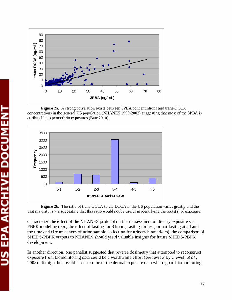
77

0102030405060708090

0 10 20 30 40 50 60 70 80

3PBA (ng/mL)

tran

s-D

CC

A (n

g/m

L)

Figure 2a. A strong correlation exists between 3PBA concentrations and trans-DCCA concentrations in the general US population (NHANES 1999-2002) suggesting that most of the 3PBA is attributable to permethrin exposures (Barr 2010).

0

500

1000

1500

2000

2500

3000

3500

0-1 1-2 2-3 3-4 4-5 >5

trans-DCCA/cis-DCCA

Freq

uenc

y

Figure 2b. The ratio of trans-DCCA to cis-DCCA in the US population varies greatly and the vast majority is > 2 suggesting that this ratio would not be useful in identifying the route(s) of exposure. characterize the effect of the NHANES protocol on their assessment of dietary exposure via PBPK modeling (e.g., the effect of fasting for 8 hours, fasting for less, or not fasting at all and the time and circumstances of urine sample collection for urinary biomarkers), the comparison of SHEDS-PBPK outputs to NHANES should yield valuable insights for future SHEDS-PBPK development.

In another direction, one panelist suggested that reverse dosimetry that attempted to reconstruct exposure from biomonitoring data could be a worthwhile effort (see review by Clewell et al., 2008). It might be possible to use some of the dermal exposure data where good biomonitoring

78

data are available to test this option. If this is feasible, then look at the NHANES data and try to reconstruct the exposure and compare this with exposure generated by SHEDS. Although two different urinary concentration predictions were compared with measured values (the average excreted versus that predicted for 24 hours and that predicted for 0.5 to 2 h after a prior void time), the level of detail provided in the Agency’s presentation and subsequent discussion was insufficient even for those on the Panel with deep expertise in PBPK modeling to be certain if the comparisons of the data were reasonable. Access to the actual PBPK model prior to the meeting would have helped to critically evaluate the work and to provide more useful feedback on the work to date as well as on future directions. There were some differences in the information presented at the meeting and provided as background on the PBPK modeling that also made evaluating the work challenging. For example, the Appendix states that the partition coefficients were estimated from Schmitt et al. (2008); however, the values for deltamethrin appear to be from other sources (Tornero, 2008; Mirfazaelin, 2006). The reason for the difference in the trans- versus cis-permethrin was not given, nor was the reason for assuming a difference in permethrin and deltamethrin for the fat but not for other tissues. Nonetheless, Panelists generally support the EPA’s plans as outlined in their presentations to compare the modeling predictions with other studies such as the Child Care Centers, American Healthy Homes Survey, and the Jacksonville Florida study (Naeher et al., 2010). Another panelist suggested that the use of selected SHEDS output percentiles as inputs to PBPK would yield large computational efficiencies. For instance, if the user knew at the outset that s/he was interested in analyzing 95th percentile results from PBPK, there would be no need to use all of percentile results from SHEDS as input to the PBPK model. However, evaluation with just the NHANES data is not sufficient because it provides only a snapshot at a large, general population level. Since the SHEDS model is intended for application in regulatory settings, it should also be robust and accurate for subpopulations of highly exposed individuals (as well as the population distributions discussed in response to Charge Question 5-1c). The numerous model evaluation processes that the Panel recommends in response to Charge Question 4 are applicable here. Recommended model evaluation steps include:

1) Assessing whether the dietary model adequately captures the percentage of vegetarians as a fraction of general population (using available national-level statistics).

2) Extend Step 1 above to assess whether the dietary model adequately captures classes of different “never eat” surveys as a fraction of total general population (utilizing available dietary databases.

3) Assessing whether the statistical properties of the virtual individuals created within the model adequately capture the statistics of the input distributions.

The mechanics of sampling for comparisons seems to have value. In general, just being able to plot the NHANES observations and the model predictions on the same graph indicates that the modelers have done well and/or been very fortunate. However, the cumulative distribution plots that are currently presented in the Agency paper are far from ideal for making clear the similarities and differences between the observations and predictions. What the Panel could not determine from the Agency’s figures was whether the variability in response matches the comparison data. While the comparison of the upper percentiles provided to the Panel as Figures

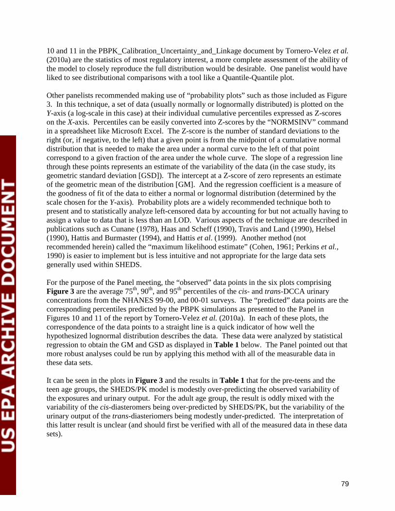
79

10 and 11 in the PBPK_Calibration_Uncertainty_and_Linkage document by Tornero-Velez et al. (2010a) are the statistics of most regulatory interest, a more complete assessment of the ability of the model to closely reproduce the full distribution would be desirable. One panelist would have liked to see distributional comparisons with a tool like a Quantile-Quantile plot. Other panelists recommended making use of “probability plots” such as those included as Figure 3. In this technique, a set of data (usually normally or lognormally distributed) is plotted on the Y-axis (a log-scale in this case) at their individual cumulative percentiles expressed as Z-scores on the X-axis. Percentiles can be easily converted into Z-scores by the “NORMSINV” command in a spreadsheet like Microsoft Excel. The Z-score is the number of standard deviations to the right (or, if negative, to the left) that a given point is from the midpoint of a cumulative normal distribution that is needed to make the area under a normal curve to the left of that point correspond to a given fraction of the area under the whole curve. The slope of a regression line through these points represents an estimate of the variability of the data (in the case study, its geometric standard deviation [GSD]). The intercept at a Z-score of zero represents an estimate of the geometric mean of the distribution [GM]. And the regression coefficient is a measure of the goodness of fit of the data to either a normal or lognormal distribution (determined by the scale chosen for the Y-axis). Probability plots are a widely recommended technique both to present and to statistically analyze left-censored data by accounting for but not actually having to assign a value to data that is less than an LOD. Various aspects of the technique are described in publications such as Cunane (1978), Haas and Scheff (1990), Travis and Land (1990), Helsel (1990), Hattis and Burmaster (1994), and Hattis et al. (1999). Another method (not recommended herein) called the “maximum likelihood estimate” (Cohen, 1961; Perkins et al., 1990) is easier to implement but is less intuitive and not appropriate for the large data sets generally used within SHEDS. For the purpose of the Panel meeting, the “observed” data points in the six plots comprising Figure 3 are the average 75th, 90th, and 95th percentiles of the cis- and trans-DCCA urinary concentrations from the NHANES 99-00, and 00-01 surveys. The “predicted” data points are the corresponding percentiles predicted by the PBPK simulations as presented to the Panel in Figures 10 and 11 of the report by Tornero-Velez et al. (2010a). In each of these plots, the correspondence of the data points to a straight line is a quick indicator of how well the hypothesized lognormal distribution describes the data. These data were analyzed by statistical regression to obtain the GM and GSD as displayed in Table 1 below. The Panel pointed out that more robust analyses could be run by applying this method with all of the measurable data in these data sets. It can be seen in the plots in Figure 3 and the results in Table 1 that for the pre-teens and the teen age groups, the SHEDS/PK model is modestly over-predicting the observed variability of the exposures and urinary output. For the adult age group, the result is oddly mixed with the variability of the cis-diasteromers being over-predicted by SHEDS/PK, but the variability of the urinary output of the trans-diasteriomers being modestly under-predicted. The interpretation of this latter result is unclear (and should first be verified with all of the measured data in these data sets).

80

Figure 3. Six probability plots of only the 75th, 90th, and 95th percentile of NHANES observed and Tornero-Velez et al. (2010a) predicted urinary concentrations of permethrin metabolites. Plots of data for the cis isomer are on the left, while plots of data for the trans isomer are on the right. From top to bottom, the plots show data for preteen, teen, and adult age groups.

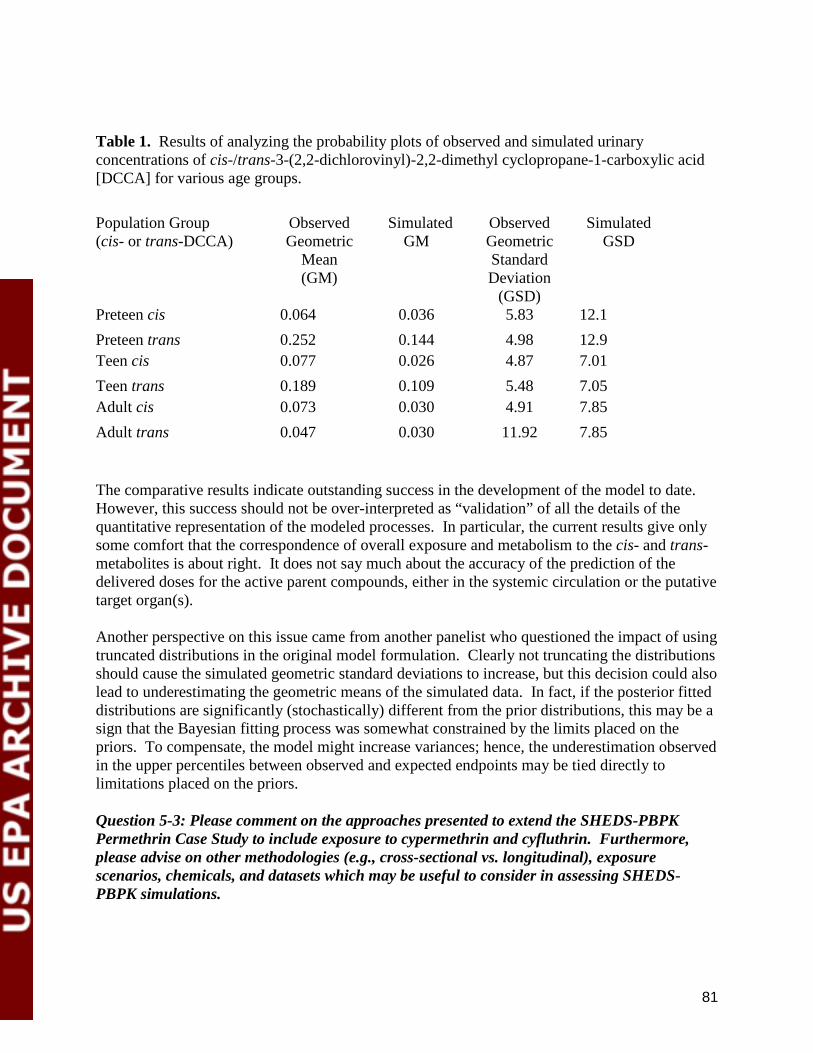
81

Table 1. Results of analyzing the probability plots of observed and simulated urinary concentrations of cis-/trans-3-(2,2-dichlorovinyl)-2,2-dimethyl cyclopropane-1-carboxylic acid [DCCA] for various age groups.

Population Group (cis- or trans-DCCA)

Observed Geometric

Mean (GM)

Simulated GM

Observed Geometric Standard Deviation

(GSD)

Simulated GSD

Preteen cis 0.064 0.036 5.83 12.1 Preteen trans 0.252 0.144 4.98 12.9 Teen cis 0.077 0.026 4.87 7.01 Teen trans 0.189 0.109 5.48 7.05 Adult cis 0.073 0.030 4.91 7.85 Adult trans 0.047 0.030 11.92 7.85 The comparative results indicate outstanding success in the development of the model to date. However, this success should not be over-interpreted as “validation” of all the details of the quantitative representation of the modeled processes. In particular, the current results give only some comfort that the correspondence of overall exposure and metabolism to the cis- and trans- metabolites is about right. It does not say much about the accuracy of the prediction of the delivered doses for the active parent compounds, either in the systemic circulation or the putative target organ(s). Another perspective on this issue came from another panelist who questioned the impact of using truncated distributions in the original model formulation. Clearly not truncating the distributions should cause the simulated geometric standard deviations to increase, but this decision could also lead to underestimating the geometric means of the simulated data. In fact, if the posterior fitted distributions are significantly (stochastically) different from the prior distributions, this may be a sign that the Bayesian fitting process was somewhat constrained by the limits placed on the priors. To compensate, the model might increase variances; hence, the underestimation observed in the upper percentiles between observed and expected endpoints may be tied directly to limitations placed on the priors. Question 5-3: Please comment on the approaches presented to extend the SHEDS-PBPK Permethrin Case Study to include exposure to cypermethrin and cyfluthrin. Furthermore, please advise on other methodologies (e.g., cross-sectional vs. longitudinal), exposure scenarios, chemicals, and datasets which may be useful to consider in assessing SHEDS-PBPK simulations.

82

The Panel concluded that the Agency’s underlying concept and the tools (i.e., PBPK model in combination with SHEDS) were fundamentally sound. However, further extending the PBPK-SHEDS model to fit other pyrethroids will require adding increased complexity to the model to cope with a myriad of issues. While most panelists agreed that such an expanded model would be of great value, such an expansion may be feasible only for levels of exposure sufficiently low such that interactions, saturation, and induction are avoided. To model exposures beyond the normal low chronic levels to include high percentiles or acute effects, then the complexity of the model will increase the challenge of developing it. The Panel indicated that the Agency provided a case study of a simple, single chemical analysis of a model that is both elegant and parsimonious, and able to utilize SHEDS output as a separate component to its modeled clearance. On the one hand, the Agency’s plans to extend this PBPK model for mixtures of chemicals assessed simultaneously is to be applauded since ultimately this represents real-world environmental exposure-ADME considerations. On the other hand, the Panel identified a number of issues that should be considered further before the model can be used for mixtures. To begin with, there is no consideration of the possible effects of reversible inhibition through the use of multiple chemicals that utilize the same metabolic pathways. Primarily, the Agency should consider very carefully the potential of competitive metabolic inhibition and its affect on the predicted total clearance of each compound. Other paths that may cause saturation of enzyme capacity (such as noncompetitive or slow-tight inhibition) are rarer, but may also occur. There are several examples of drugs and chemicals that alter each other’s metabolism within relatively short periods, either contributing to or altering toxicity (e.g., alcohol potentiation of acetaminophen toxicity) at both the protein and transcriptional levels. The above points are to be taken doubly seriously in the case of infants and young children (particularly under two years of age) due to the inadequacy of several CYP detoxification enzymes (notably CYP3A4) that are major paths of clearance metabolism for these compounds. Furthermore, Phase II metabolism has not been considered and at least for the UDP-glucuronosyl transferases, a similarly delayed developmental profile also exists for infants. Further, the model currently does not have ability to take into account polymorphisms and their very real potential to affect clearance. Polymorphism is extremely important for the pyrethroids where CYP paths of metabolism include CYP2C and CYP3A isoforms. Polymorphic individuals with low metabolism capacity of these enzymes likely represent a small but distinct population with increased risk. Additionally, while animal data is commonly extrapolated to humans, caution must be exercised where there are known differences in metabolic pathways between species (Cao et al., 2006). Many examples of this exist for drugs and environmental toxicants. An example is for the drug methamphetamine. The Phase I metabolism of methamphetamine is performed by cytochromes P450 1A2, 2D6 and 3A4 in humans and CYP1A2, 2D1 and 3A2 in rodents (de la Torre, 2004) Additionally, important sex and species differences in conjugation have been reported such that in rodents the glucuronide pathway predominates and females show higher UGT activity, while in humans sulfonylation is the major detoxicative pathway (Sever, 1976). This is a concrete example where the extrapolation of metabolic data from rodents to humans may be inaccurate; therefore proposals to inform these models with non-human metabolic data need to be carefully evaluated.

83

And finally, there is the complication that the presence of enantiomers causes the number of submodels (and their parameters) required within such a model to multiply rapidly. In addition to differences in the metabolism of enantiomers of the parent compound, there is the difference in the metabolism of each of these enantiomers and the potential for preformed enantiomers to be created within the environmental residue. Enantiomer-specific information has been derived from air samples (Williams et al., 2006). The Panel agreed that because a wide range of pharmacokinetic profiles has been observed among the pyrethroids, it will probably be necessary to develop models for each compound. Parameterizing each model would be onerous and very complex given the number of pyrethroids, isomers, and enantiomers. If the intention is to generalize the SHEDS-PBPK model to a wider range of pyrethroids, then it might be worthwhile to use a quantitative structure property relationship approach to predict some of the parameters. Should interactions occur between compounds (as described above), then this would be a problem irrespective of the approach to modeling the mixtures. If the effects of the compounds (in a mixture) are additive, then both modeling and interpretation would be simpler as shown in the work of Timchalk and Poet (2008) on a mixture of chlorpyrifos and diazinon. Many precautions for addressing multiple chemical exposures were discussed. One possible approach to incorporate many pyrethroids into future SHEDS-PBPK modeling development is to adapt the Relative Potency Factor (RPF) approach that is being used for the Agency’s organophosphate cumulative risk assessment. Understanding that there is a lack of a single parameter to characterize the common toxicological mechanism applicable to pyrethroid exposure, the implementation of the RPF approach for pyrethroids might be problematic. For a cumulative risk scenario, the option of applying the RPF before the linkage of exposure from SHEDS to the PBPK model was suggested. However, due to the unique pharmacokinetic characteristics of each pyrethroid, it would be more logical to apply RPF after accounting for these factors. The Panel noted that simply incorporating three pyrethroids into the SHEDS-PBPK model (as proposed) is not adequate to predict overall pyrethroid exposure at the population level. The use pattern of pyrethroids both in agricultural and residential environments is constantly changing, and the use of other pyrethroids may become common in the future, whereas the use of the three pyrethroids being proposed may diminish due to insect resistance or other reasons. For instance, the use of bifenthrin in agriculture and in residential pest control applications has gained in popularity since 2007. The addition of deltamethrin in outdoor wood preservatives and other pyrethroids in paints are other examples of uses that have emerged. The structure of the present PBPK model could be adapted for multi-chemical pharmacokinetics. An integrated model structure that utilizes simple parameterizations of metabolic interactions (both inhibition as well as induction of metabolism) would allow for a systematic refinement of a mixture’s pharmacokinetics. The current focus of evaluation processes on chronic exposures to the general population is necessary, but clearly not sufficient. The Panel recommended that additional evaluations be performed on field study data based on populations in geographic areas

84

corresponding to high exposures (e.g., the Jacksonville study). Eventually, the model should be evaluated for its ability to model acute occupational exposures.

85

REFERENCES

Anderson BJ, Holford NH. 2009. Mechanistic basis of using body size and maturation to predict clearance in humans. Drug Metab Pharmacokinet 24(1):25-36.

Appela, K., Gundert-Remya, U, Fischera H., Fauldeb M., Mrossc KG, Letzeld S, Rossbachd B. 2008. Risk assessment of Bundeswehr (German Federal Armed Forces)permethrin-impregnated battle dress uniforms (BDU). Int J Hyg Environ Health 211:88-104.

ATSDR (Agency for Toxic Substances and Disease Registry). 2003. Toxicological profile for pyrethins and pyrethroids. Atlanta, GA. Available at: http://www.atsdr.cdc.gov/toxprofiles/tp155.pdf)

Barr DB, Angerer J. 2006. Potential uses of biomonitoring data: A case study using the organophosphorous pesticides chlorpyrifos and malathion. Environ Health Perspect 114:1763-1769.

Barr DB, Olsson AO, Wong LY, Udunka S, Baker SE, Whitehead RD, Magsumbol MS,

Williams BL, Needham LL. 2010. Urinary concentrations of metabolites of pyrethroid insecticides in the general U.S. population: National Health and Nutrition Examination Survey 1999-2002. Environ Health Perspect 118(6):742-748.

Bradman A, Whyatt RM. 2005. Characterizing exposures to nonpersistent pesticides during

pregnancy and early childhood in the National Children's Study: A review of monitoring and measurement methodologies. Environ Health Perspect 113(8):1092-1099.

Butt CM, Diamond ML, Truong J, Ikonomou MG, ter Schure AF. 2004. Spatial distribution of

polybrominated diphenyl ethers in southern Ontario as measured in indoor and outdoor window organic films. Environ Sci Technol 38(3):724-31.

Butte W, Heinzow B. 2002. Pollutants in house dust as indicators of indoor contamination. Rev

Environ Contam Toxicol 175:1-46. Cao X, Gibbs ST, Fang L, Miller, HA, Landowski CP, Shin H-C, Lennernas H., Zhong Y,

Amidon G., Yu LX, Sun D. 2006. Why is it challenging to predict human intestinal drug absorption and oral bioavailability in human using rat model. Pharm Res 23:1675-1686.

Clewell HJ, Tan YM, Campbell JL, Andersen ME. 2008. Quantitative interpretation of human

biomonitoring data. Toxicol Appl Pharmacol 231:122-133. Cohen AC. 1961.Tables for maximum likelihood estimates: Singly truncated and singly

censored samples, Technometrics 3(4):535-541.

Cunnane C. 1978. Unbiased plotting positions--A review. J Hydrol 37:205-222.

86

de la Torre R, Farré M, Roset PN, Pizarro N, Abanades S, Segura M, Segura J, Camí J. 2004. Human pharmacology of MDMA: pharmacokinetics, metabolism, and disposition. Ther Drug Monit 26(2):137-44.

Fortin M-C, Bouchard M, Carrier G, Dumas P. 2008. Biological monitoring of exposure to pyrethrins and pyrethroids in a metropolitan population of the Province of Quebec. Canada Environ. Res 107:343-350.

Haas C N, Scheff PA. 1990. Estimation of averages in truncated samples. Environ Sci Technol 24(6):912-919.

Hattis D, Banati P, Goble R, Burmaster D. 1999. Human interindividual variability in parameters related to health risks. Risk Anal 19:705-720.

Hattis D Burmaster DE. 1994. Assessment of variability and uncertainty distributions for practical risk analyses. Risk Anal 14:713-730.

Hattis D., Lynch MK. 2007. Empirically observed distributions of pharmacokinetic and pharmacodynamic variability in humans—implications for the derivation of single point component uncertainty factors providing equivalent protection as existing RfDs. In: Toxicokinetics in Risk Assessment, J. C. Lipscomb and E. V. Ohanian, eds., Informa Healthcare USA, Inc., pp. 69-93.

Hays SM, Aylward LL, Gagné M, Nong A, Krishnan K. 2010. Biomonitoring equivalents for inorganic arsenic. RegulToxicol Pharmacol 58(1):1-9.

Hays SM, Aylward LL, Gagné M, Krishnan K. 2009. Derivation of biomonitoring equivalents for cyfluthrin. RegulToxicol Pharmacol 55:268-275.

Hays SM, Aylward LL, LaKind JS, Bartels MJ, Barton, HA, Boogaard PJ, Brunk C, DiZio S, Dourson M, Goldstein DA, Lipscomb J, Kilpatrick ME, Krewski D, Krishnan K, Nordberg,M, Okino M, Tan Y-M, Viau C,Yager J. 2008. Guidelines for the derivation of biomonitoring equivalents: Report from the biomonitoring equivalents expert workshop. RegulToxicol Pharmacol 51:S4-S15.

Helsel DR. 1990. Less than obvious: Statistical treatment of data below the detection limit. Environ Sci Technol 24(12):1766-1774.

Kim K-B, Anand SS, Muralidhara S, Kim HJ,Bruckner JV. 2007. Formulation-dependent toxicokinetics explains differences in the GI absorption, bioavailability and acute neurotoxicity of deltamethrin in rats. Toxicology 234: 194–202.

Kissel JC. 2010. The mismeasure of dermal absorption. J Expo Sci Environ Epidemiol 2010 Apr 28. [Epub ahead of print doi:10.1038/jes.2010.22]

Lu C, Barr DB, Pearson M, Bartell S, Bravo R. 2006a. A longitudinal approach to assessing urban and suburban children's exposure to pyrethroid pesticides. Environ Health Perspect 114(9):1419-23. PMID: 16966099.

87

Lu C, Toepel K, Irish R, Fenske RA, Barr DB, Bravo R. 2006b. Organic diets significantly lower children's dietary exposure to organophosphorus pesticides. Environ Health Perspect 114(2): 260-263. PMID: 16451864.

Lu C, Barr DB, Pearson MA, Waller LA. 2008. Dietary intake and its contribution to the longitudinal organophosphorus pesticide exposure in urban and suburban children. Environ. Health Perspect 116(4)537:542. PMID: 18414640.

Lu C, Barr DB, Pearson MA, Waller LA. 2009. The attribution of urban and suburban children’s exposure to synthetic pyrethroid pesticides: a longitudinal assessment. J Exp Sci Environ Epidemiol 19(1):69-79. PMID: 18766203.

Mirfazaelian A, Kim KB, Anand SS, Kim HJ, Tornero-Velez R, Bruckner JV, Fisher JW.2006. Development of a physiologically based pharmacokinetic model for deltamethrin in the adult male Sprague-Dawley rat. Toxicol Sci 93:432 – 442.

Morgan MK, Sheldon LS, Croghan CW, Jones PA, Chuang JC, Wilson NK. 2007. An observational study of 127 preschool children at their homes and daycare centers in Ohio: environmental pathways to cis- and trans-permethrin exposure. Environ Res 104(2):266-274.

Naeher LP, Barr DB, Rithmire N, Edwards J, Holmes AK, Needham LL, Rubin CS. 2009. Pesticide exposure resulting from treatment of lice infestation in school-aged children in Georgia. Environ Int 35:358–362.

Naeher LP, Tulve NS, Egeghy PP, Barr DB, Adetona O, Fortmann RC, Needham LL, Bozeman E, Hilliard A, Sheldon LS. 2010. Organophosphorus and pyrethroid insecticide urinary metabolite concentrations in young children living in a southeastern United States city. Sci Total Env 408:1145–1153.

Oakley J, O’Hagan A. 2004. Probabilistic sensitivity analysis of complex models: a Bayesian approach. Journal of Royal Statistical Society Series B - Statistical Methodology 66:751–769.

Perkins JL, Cutter GN, Cleveland, MS. 1990. Estimating the mean, variance, and confidence limits from censored (< limit of detection), lognormally-distributed exposure data. Amer Ind Hyg Assoc J 51(8):416-419.

Prater MR, Gogal Jr RM, Blaylock BL, Longstreth J, Holladay SD. 2002. Single-dose topical exposure to the pyrethroid insecticide, permethrin in C57BL/6N mice: effects on thymus and spleen. Food Chem Toxicol 40: 863-1873.

Özkaynak H, Xue J, Zartarian V, Glen G, Smith L. 2010. Modeled estimates of soil and dust ingestion rates for children. Risk Analysis, In Press.

Popendorf W. 1990. The effects of organophosphate insecticide residue variability upon reentry intervals. Amer J Ind Med 18(3):313-319.

88

R Development Core Team. 2009. R: A language and environment for statistical computing. R Foundation for Statistical Computing,Vienna, Austria. ISBN 3-900051-07-0, URL http://www.R-project.org.

Riederer AM, Bartell SM, Barr DB, Ryan PB. 2008. Diet and nondiet predictors of urinary 3-phenoxybenzoic acid in NHANES 1999-2002. Environ Health Perspect 116(8):1015-1022. Erratum in: Environ Health Perspect 116(8):1021.

Rossbach B, Appel KE, Mross KG, Letzel S. 2010. Uptake of permethrin from

impregnated clothing. Toxicol Lett 15:192(1):50-55.

Saltelli A, Ratto M, Andres T, Campolongo F, Cariboni J, Gatelli D, Saisana M.Tarantola S. 2008. Global Sensitivity Analysis. The Primer, John Wiley and Sons.

SAP (FIFRA Scientific Advisory Panel) 2007. A Set of Scientific Issues Being Considered by the Environmental Protection Agency Regarding: Review of EPA/ORD/NERL's SHED-Multimedia Model Aggregate version 3, August 14-15, 2007, Arlington, VA.

Sever PS, Dring LG, Williams RT. 1976. Urinary metabolites of p-hydroxyamphetamine in man, rat and guinea-pig. Xenobiotica 6(6):345-353.

Smith NS, Campbell JA, Busby-Hjerpe AL, Lee S, Poet TS, Barr DB.Timchalk C. 2009. Comparative chlorpyrifos pharmacokinetics via multiple routes of exposure and vehicles of administration in the adult rat. Toxicology 261:47-58.

Sobol IM, Tarantola S, Gatelli D, Kucherenko S and Mauntz W. 2007. Estimating the approximation error when fixing unessential factors in global sensitivity analysis . Reliability Engineering and System Safety 92:957–960.

Timchalk C, Nolan RJ, Mendrala, AL, Dittenber DA, Brzak KA, Mattsson JL. 2002. A physiologically based pharmacokinetic and pharmacodynamic model for the organophosphate insecticide chlorpyrifos in rats and humans. Toxicol Sci 66:34-53.

Timchalk C, Poet TS. 2008. Development of a physiologically based pharmacokinetic and pharmacodynamic model to determine dosimetry and cholinesterase inhibition for a binary mixture of chlorpyrifos and diazinon in the rat. Neurotox 29:428-443.

Tomalik-Scharte D, Lazar A, Meins J, Bastian B, Ihrig M, Wachall B, Jetter A, Tantcheva-Poór I, Mahrle G, Fuhr U. 2005. Dermal absorption of permethrin following

topical administration. Eur J Clin Pharmacol 61(5-6):399-404.

Toni T, Stumpf MPH. 2010 Simulation-based model selection for dynamical systems in systems and population biology. Bioinformatics 26:104-110.

Tornero-Velez R, Davis J, Xue J, Setzer RW. 2010a. Physiologically-Based Pharmacokinetic Models of Pyrethroids: Bayesian Calibration and Their Use in Interpreting Probabilistic Exposure Data. Agency background document found in Regulations.gov, Docket: EPA-HQ-OPP-2010-0383.

89

Tornero-Velez R, Mirfazaelian A, Kim KB, Anand SS, Kim HJ, Haines WT, Bruckner JV, Fisher JW. 2010b. Evaluation of deltamethrin kinetics and dosimetry in the maturing rat using a PBPK model. Toxicol Appl Pharmacol 244:208-217.

Travis CC, Land, ML. 1990. Estimating the mean of data sets with nondetectable values. Environ Sci Technol 24(7):961-962.

USEPA (United States Environmental Protection Agency). 2010. August 2007 FIFRA Scientific Advisory Panel Recommendations for SHEDS-Dietary and SHEDS-Residential Modules (Summarized) and EPA Responses, Background Material for July 20-22 2010 FIFRA Scientific Advisory Panel Meeting. Agency background document found in Regulations.gov, Docket: EPA-HQ-OPP-2010-0383.

Williams MK, Barr DB, Camann DE, Cruz LA, Carlton EJ, Borjas M, Reyes A, Evans D, Kinney PL, Whitehead RD Jr, Perera FP, Matsoanne S, Whyatt RM. 2006. An intervention to reduce residential insecticide exposure during pregnancy among an inner-city cohort. Environ Health Perspect 114(11): doi:10.1289/ehp.9168.

Woollen BH, Marsh JR, Laird WJ, Lesser JE. 1992. The metabolism of cypermethrin in man: differences in urinary metabolite profiles following oral and dermal administration. Xenobiotica 22(8):983-91.

Xu Y, Hubal EA, Clausen PA, Little JC. 2009. Predicting residential exposure to phthalate plasticizer emitted from vinyl flooring: a mechanistic analysis. Environ Sci Technol 43(7):2374-80.

Xu Y, Cohen Hubal EA, Little JC. 2010. Predicting residential exposure to phthalate plasticizer emitted from vinyl flooring: sensitivity, uncertainty, and implications for biomonitoring. Environ Health Perspect 118(2):253-8.

Zhang X, Diamond ML, Ibarra C, Harrad S. 2009. Multimedia modeling of polybrominated diphenyl ether emissions and fate indoors. Environ Sci Technol 43(8):2845-50.

Zheng J, Frey HC. 2004. Quantification of variability and uncertainty using mixture distributions: Evaluation of sample size, mixing weights, and separation between components. Risk Anal 24: 553-71.

90

Appendix I : Editorial Comments regarding the use of “Scenario” in the SHEDS-Residential User Manual One Panel member discussed three different variations in the meaning of “scenario” used in the SHEDS-Residential User Manual. The first use of the term “scenario” is clearer because there is more information to determine its specific meaning. The second use of the term “scenario” is in conjunction with “application,” i.e., application scenario or scenario application method. The third use of the term “scenario” is in conjunction with “type” or “category,” i.e., “scenario type” or “scenario category.” Use of “scenario” in the second and third cases is less specific than in the first case. A detailed list of each of the “scenario” cases is found below [scenario is underlined for emphasis]

, page numbers are from the SHEDS-Residential User Manual.

page 2: SHEDS version 4 allows consideration of multiple chemicals per model run. The

user may also select several scenario categories (each containing one or more of the different chemicals) to be analyzed together in the same run. The model permits the use of co-occurrence factors that control the likelihood of the various scenarios being applied at the same house at the same time. The human exposure results are automatically aggregated across the scenarios

used in the given model run. The cumulative exposure results for all chemicals in the simulation are also determined.

page 3: The user has the ability and the responsibility to configure SHEDS to a particular scenario(s) of interest. This includes specifying the target population, the simulation period, the chemical and application method(s) of interest, and the distributions for many model parameters. The model allows the user to select one or more scenario application methods

from a pre-determined list in the GUI.

page 6: Some sections will need to be revisited a number of times to enter all information. In particular, the sections defining application details and dates, and those defining media concentrations will need to be defined for each application or scenario type

being simulated.

page 25: Specify Application Scenarios: Specify the application scenarios

to be used in the run. Define the dates and times of applications, reentry times, and relationships between application dates.

page 35: There are three options to generate residues and concentrations for scenario-relevant media

:

page 38: The user must also select Specify Parameters before clicking the Specify Inputs button on the Specify Application Scenario Details screen for each scenario

for which co-occurrence inputs are to be specified.

page 41: 5.7 Specify Application Scenarios Simulated. Clicking on “Specify Application Scenarios” on the main screen begins a series of screens through which the user

91

must navigate in their entirety before returning to the main screen. The exact screens vary depending on options selected. See Figure 2.1 for an overview of the screens in this section. The following screens may be visited: The first screen is used to identify the scenarios to be simulated. [Several lines with multiple uses of "scenario

" follow this paragraph within the User Guide.]

page 42: 5.7.1 Specify Application Scenarios. The specific scenarios or applications

to be simulated are specified on this screen (Figure 5.17).

page 42-3: There are nine pre-defined application scenarios

available in SHEDS. These appear in the Scenario Library. The available scenarios and their locations are as follows: [a list is provided in the document]

page 44: 5.7.2 Specify Exposure Scenario Details. Once all application scenarios for a run have been selected, the user proceeds to the Specify Exposure Scenario

Details screen (Figure 5.19).

page 55: The following are the required distributions for each type of scenario

: [list provided in text]

page 57: The user must define these four distributions for each medium affected by each scenario for each chemical. Once an application is made for a scenario, these distributions will determine the concentrations on each medium. When another application is made in the same scenario, the first distribution is used once again; there is no persistence of chemical from the previous application. The concentrations on a medium from different scenarios are added when determining exposure of an individual. The background values are assumed to be included in the distributions; the user cannot define background concentrations on media not included in the scenarios

.