Are Housing Prices Pulled Down or Pushed Up by Fracked Oil and Gas Wells?

A Hedonic Price Analysis of Housing Values in Weld County, Colorado

Ashley Bennett John Loomis

Dept of Agricultural and Resource Economics Colorado State University

Fort Collins, CO 80523-1172 August 22, 2014

Accepted for Publication in Society & Natural Resources

Running Head: House Prices and Fracking Please address correspondence to: Dr. John Loomis, Professor John.Loomis@colostate.edu Acknowledgements

We would like to thank Courtney Anaya, Weld County Assessor’s Office for providing the sales data. Comments and suggestions were provided by Dr. Costanigro, Dr. Reich, Dr. Haefele and Brian Quay. Of course none of these individuals are responsible for the content. The responsibility for the analysis and conclusions lies with the authors. The findings represented are those of the authors and do not necessarily represent those of Colorado State University.

[1]

Introduction

Hydraulic fracturing, also commonly known as “fracking,” has made possible oil and gas

production in geographic areas that have not traditionally seen such oil and gas drilling.

Fracking involves pumping fracking fluids – a mixture of water and chemicals – into the well at

a high pressure to fracture the shale formation (EPA, 2011). Given that widespread use of these

techniques, particularly in and around urban areas, is still relatively new there is little existing

literature on the costs and benefits of fracking on property values.

Perhaps due in part to the lack of peer-reviewed research on the subject, there has been a

noteworthy amount of public debate about potential risks to public health and water sources

taking place in the media. As fracking has moved into suburban and urban areas of

Pennsylvania, Ohio, and Colorado, citizens have mobilized into active opposition. This resulted

in voter referenda ranging from five year time outs to outright bans in towns in Ohio and in

Colorado, several of which passed in November 2013’s elections. For example, Fort Collins,

Colorado passed a “time out” in order for studies of the effects of fracking “on property values

and human health” to be conducted (Coloradoan, 11-7-2013).

However, one issue that has been brought up in the debate on fracking is that there are

beneficial economic impacts of oil/gas exploration on local economies in the form of increased

employment in oil and gas sectors. The increased workforce and subsequent increased demand

for housing in the area may be driving housing values up as it has in areas of North Dakota

(Platt, 2013).

Alternatively, environmental and health risks associated with hydraulic fracturing,

including water quality and quantity issues and air and noise pollution, may be capitalized into

housing prices of homes located near drilling sites pushing housing prices down. There has been

little peer reviewed research of this net effect.

[2]

Exactly what are these environmental and health impacts of major concern? These

impacts include noise and nighttime lights associated with the round the clock drilling of a well

and associated truck traffic bringing water/drilling fluid to the site. In addition there are concerns

about air quality and potential risks to water sources. McKenzie et al. (2012) studied health

effects resulting from air emissions generated in the process of unconventional natural gas

development; they found that those living within a half-mile or less of unconventional natural

gas development are at greater risk for negative health effects than are those living farther than a

half-mile from it. This half-mile radius is useful in this study to help guide spatial delineation of

the effects of fracking on housing prices.

A consensus as to whether shale exploration will help or harm the communities in which

it is taking place has not yet been reached, indicating that further research in on the topic is

imperative in order to construct informed policy on the issue. This is especially true since most

studies have not compared the impacts of drilling in urban and rural areas.

The goal of this study is to expand the literature on the effects oil and gas activity on

property values in the leading Colorado county for fracking, Weld County. With the largest share

of both active and permitted wells in the state, and given its mix between urban and rural areas

paired with a relatively high number of housing transactions, Weld County provides an

interesting opportunity to look at the effects fracking is having on those residing near the drilling

sites. Weld County is a very large county in northeastern Colorado bordered by Kansas and

Nebraska with a relatively large city (Greeley), surrounded by a suburban area, and a spread of

many rural towns. An analysis comparing the influx of drill sites on sale values of homes in the

surrounding area is something that has the potential to be useful to policy makers, local

government officials, and the general voting public as it deliberates votes on bans or “time outs”

on fracking.

[3]

Literature Review

Hedonic Price Model

A standard economic model to determine the economic effects of changes in

environmental quality near residential housing areas is the Hedonic Price Model (HPM). The

intuition behind this method is as follows. High amenity areas are both desirable places to live

and scarce in supply. Those properties with access to these desirable attributes find their house

prices bid up by competing buyers willing to pay more to live near high environmental

amenities. Likewise, in order to get households to accept living near a less desirable environment

(e.g., oil/gas well), households have to be compensated by lower house prices. As noted in this

journal, positive amenities such as forests (Kim and Johnson, 2002) and natural amenities such

as lakes (White and Leefers, 2007) have a positive effect on house prices, while flammable

building materials on houses located in WUI areas had a negative effect on property values

(Champ, et al. 2010).

Inter-regional wage differentials can also signal differences in amenities and disamenities

associated with living in a particular area (Roback, 1982, 1988). The logic is just the same as the

housing price model, but in the opposite direction. Since few workers want to live in a less

desirable area, wages have to be made higher to attract them. This is one of the bases of the wage

hedonic model (See Freeman 2003 for more discussion).

Thus, ideally, if one were interested in explaining interurban wage differentials and house

price differentials, the study would analyze both markets. Such a model is beyond the scope of

our paper (and the existing literature on effects of oil and gas production) but would be an

important advancement in this area. This is especially true for areas experiencing oil and gas

“booms” since the sudden abundance of employment often pushes wages up, attracting workers,

which in turn increases demand for, and thus the price of housing despite the arguable

disamenities associated with the drilling boom.

[4]

Due to space constraints, we just summarize the essential elements of the hedonic price

model. The details of the utility theory underlying the hedonic model are discussed by Freeman

(2003) and by Taylor (2003). Let Z represent a house with a bundle of attributes, Z = z1, z2, z3,

… zn. Hedonic models start with the assumption that a consumer (j) derives utility (U) from the

differentiated good (Z) and the composite commodity (X) that symbolizes all other goods.

(2.1) Uj =( X; z1, z2, z3, … zn)

The budget constraint is: yj = x + P(Z), where P(Z) represents the hedonic price function.

The consumer maximizes utility by choosing the amounts of X and zi subject to his or her budget

constraint. Amounts of X and zi are chosen such that the marginal rate of substitution between

any attribute, zi, and X is equal to the implicit price ratio for zi.

(2.2) ∂U/∂zi ∂P(Z) = [P(zi)] ∂U/∂X = ∂zi

Utility derived from housing is a function of the house’s structural and property

characteristics (H1…Hh), demographics and neighborhood characteristics (N1…Nn), and

location-based characteristics such as proximity to certain amenities or disamenities (L1…LL).

Housing is an increasing function of structural and property characteristics (i.e. UH > 0), an

increasing function of proximity to amenities UL >0, and a decreasing function of proximity to

disamenities UL < 0 (Loomis, 2004; Taylor, 2003). The hedonic price function in its general

form:

The simplified linear functional form is:

By regressing the attributes from the right-hand side of equation (2.4) on the dependent

variable, sales price, the implicit prices for each attribute are obtained. The regression

[5]

coefficients, βi, yielded by the regression with a linear functional form, measure the incremental

change in housing sales price due to a change in one characteristic while holding all others

constant. Thus the βi’s are the implicit prices for one more or one less unit of the particular

attribute of the house, neighborhood or local environment (amenity or disamenity).

For these implicit prices to reflect marginal willingness to pay, several assumptions are

required (Freeman, 2003). A key one for this study is that the housing market is in equilibrium.

As one might suspect, changes in future expectations about the housing market can affect the

amount a household will pay today for a house. Freeman (2003: 367) notes that “Divergences

from full equilibrium of the housing market in many circumstances will only introduce random

noise into the estimates of the MWTPs” (marginal willingness to pay). However, Freeman

indicates that there can be systematic effects on MWTP’s if existing property owners have

systematic future expectations that are not reflected in the current levels of the attribute

variables. In our case, property owners might expect oil and gas employment will push up house

prices in the future. Since neither Freeman nor others have proposed a model to incorporate

systematic future expectations into hedonic pricing models, such a model would be an important

area for significant methodological advancement, but is well beyond the scope of this applied

paper. In absence of such a model, Freeman suggests the analyst be “cautious” when using cross

section data when market forces may be changing “rapidly” (though he comments that “rapidly”

is a rather imprecise term). In our case study, we attempt to control for any systematic trends in

the housing market by including year fixed effect dummies in our model.

Applications of HPMs to similar topics

Numerous previous studies exist that investigate the impact that local disamenities have

on housing prices (see Taylor (2003) or Freeman (2003) for more discussion). However, very

few HPM studies on the impact of proximity to oil and gas wells have been done (Boxall et al.,

2005; BBC, 2006; Gopalkrishnan and Klaiber, 2014; Muehlenbachs et al., 2014). These four

[6]

studies all find negative impacts on housing values across the different types of model

specification and estimation techniques.

Boxall et al. (2005) examined the impact of small and medium-sized oil and gas facilities

on residential property values in rural areas of Alberta, Canada. Count variables for the number

of wells within four kilometers of a property were used in addition to a continuous distance

variable for the nearest sour gas plant to the house to explore whether proximity to oil and gas

facilities affects housing values. Measures of hazard and disamenity were found to have

statistically significant, negative effects on housing values, reducing the value by between 4%

and 8% at the mean level of facilities within four kilometers.

BBC (a consulting firm in Denver) conducted a hedonic price study of oil and gas wells

in Garfield County, Colorado. This county is a fairly arid rural area, with mostly ranching in

rugged country along a major east-west interstate highway. The area had undergone an oil and

gas boom during the mid 2000’s. Their simple hedonic price analysis shows that for a typical 40

acre parcel there was between a 7% and 15% reduction in house price due to the presence of a

well on the property itself. This situation is different from the concern in many areas where the

well is adjacent to residential properties, but their study does provide an estimate of the upper

bound of effects.

Gopalkrishnan and Klaiber (2014) utilized a hedonic model to assess whether any

potential negative externalities associated with fracking are capitalized into the values of

surrounding residential properties in Washington County, PA. They assessed the potential

negative effects of the information revelation that occurs between the permit approval and actual

drilling of the well. They found that using a spatial buffer of 0.75 miles and a time window six

months prior to sale that drilling had a statistically significant but small (-1.4% to -2.1%)

negative effect on properties not on well water that persists on into the six-month time window.

They indicated that the effect of drilling seemed to disappear if the drill site was two miles or

[7]

farther from the house, even if the house relied upon well water. Overall, their results show that

housing values are negatively impacted in the short term, and that those dependent upon well

water and surrounded by agricultural land are disproportionally negatively (as large as -22%)

impacted by drilling.

Muehlenbachs et al. (2014) examined the negative externalities associated with shale gas

development across different drinking water sources in a hedonic analysis of the same county in

PA. Their study focused on the interaction between groundwater and hydraulic fracturing, and

the potential risks associated with this interaction. Their estimator is based on whether the house

is located within 2 km of a shale gas well (treatment group) or outside 2 km (control group), and

one based on whether a house is dependent on groundwater (treatment group) or not (control

group) and is within 2 km of a shale gas well. This study found that the risk of groundwater

contamination leads to a statistically significant and large reduction in the price of a house,

depending on what type of water source the house uses.

These four studies all have found negative effects from oil and gas drilling on housing

values. However, these negative values reflected a particular range of distance (e.g. 2 kilometers

used by Muehlenbachs et al. 2014 or 4 kilometers used by Boxall et al. 2005), or whether a home

that received its water from a domestic water well (Muehlenbachs et al. 2014). One of these

studies looked at the effect in rural Alberta, Canada (Boxall et al., 2005) and two looked at

Washington County, Pennsylvania (Gopalkrishnan and Klaiber 2014; Muehlenbachs et al.,

2014); one study has looked at fracking on large rural properties in remote Colorado towns, but

no studies involved urban areas on the Colorado “Front Range” with its relatively flat

topography of eastern Colorado. Although Alberta has a fairly flat topography, it lacks the high

population density of Weld County, Colorado, making a direct comparison difficult. This study

adds to the existing literature by applying a hedonic price model to Weld County, Colorado, and

then separate analyses of urban and rural parts of the County.

[8]

Empirical Specification of Hedonic Price Model

Hedonic Price Function General Specification

Equation 5 shows the general linear specification that includes drill-activity variables. As

discussed below we also estimate a semi log (logging dependent variable).

(5) HPi= β0 + β1(# Drillingt)+ β2 (#Producingt)+ β3 (O/GEmpt) + +β4 (Dist-to-Wellt)+∑(βj’sSj)+∑(βk’sNk)+e Where:

# Drillingt is the number of wells being drilled within half mile of the house at the 60 day

time period when housing purchase decisions are made 1

#Producingt is the number of already producing wells within half mile of the house at the 60

day time period when housing purchases decisions are made.

O/GEmpt is oil and gas employment in our study county at the 60 day time period when

housing purchase decisions are made

Dist-to-Wellt is the distance a house is to a well

∑(βj’sSj) are the structural characteristics of the house such as square footage, year the house

was built, whether it has a garage, etc.

∑(βk’sNk) are the neighborhood characteristics such as percent with college degrees, percent

Hispanic, percentage of the houses that are rentals, etc.

Year dummy variables are added for years 2010, 2011, and 2012 to attempt to control for any

year-to-year trends in the housing market.

1 A time period of 60 days prior to the recorded sale date (the date of the official “closing on the housing”) is

chosen to capture activity that may be taking place at the time the house purchase decision is made. As McKenzie et al. (2012) report that the disturbance of a well is highest when it is within one half mile of a house, a count variable of the number of wells being drilled within 60 days and a half mile radius of house was created, # being drilled.

[9]

As suggested by a reviewer, we include spatial fixed effects in the form of town level dummy

variables. The purpose of these is to control for unobservable differences between towns that

might not already be captured in the demographic characteristics included in the model.

Functional Form of the Hedonic Price Function

The existing literature on hedonic price functions and regression analyses tend to favor a

semi-log (i.e. a log-linear) functional form for estimating the price function (Muehlenbachs et al.,

2014; Lewis & Acharya, 2006). In addition, the analysis of functional form from Cropper et al.

(1998) also suggests the semi-log model is more robust than the more general Box-Cox

functional form in the face of common econometric problems. However, a Box-Cox test for

functional form is also run. This allows us to see if either of the linear or semi-log functional

forms are appropriate. We also calculate the marginal values from the more general Box-Cox

functional form. See Cropper et al. or Taylor for more discussion on the Box-Cox test for

functional form.

However, estimating both a linear and a semi-log non linear functional form also allows

for post-estimation testing of the sensitivity of coefficient estimates to different types of

functional forms. Linear hedonic price functions, for example, have the advantage that the βi’s on

the regression slope coefficients provide implicit prices for an incremental increase of one unit in

that specific attribute. However, this assumes that the marginal value of an additional unit of

characteristic zi is constant across all houses in the sample, which may not be true for some

characteristics. To allow for non-constant marginal prices for housing characteristics, the log of

the dependent the variable is often recommended (Cropper, et al. 1998).

Statement of Hypotheses

Theory and the results of previous studies guide the hypotheses made. Most structural

characteristics of a house are expected to have a positive effect on housing prices with the

exclusion of age, because buyers prefer new/newer houses to older homes. Lot size and

[10]

residential square footage are expected to have a non-linear relationship with price, because

housing prices are thought to increase with these variables at a decreasing rate.

Discerning the expected relationship between well-activity variables and housing sale

prices is the focus of this study. For all of the count variables – #Drilling and #Producing – the

expected relationship is negative. As the density of wells being drilled or producing wells within

a half-mile of a home increases, it is expected that the house would lose value, suggesting a

negative relationship. Distance to the nearest well being drilled within two miles and the nearest

producing well within a half-mile are also included in the model. It is expected that having a well

within that distance range has a negative impact on housing values, thus since distance is used in

the linear and semi-log specifications, the estimated coefficient should have a positive sign. As

distance to the nearest well being drilled within two miles increases, housing prices should

theoretically increase. The same logic is applied to the distance to the nearest well in production,

although the scope is smaller at one half-mile. These expectations are primarily based on the

results of Boxall et al. (2005) and Muehlenbachs et al. (2014), both of whom found negative

effects of drilling on housing values within a specified distance band.

Data

Several data sets were collected from various sources and joined together to form a

database comprising housing sales date and price, housing characteristics, location, census tract

demographics, and proximity to wells being drilled and producing wells. Data on housing sales

and characteristics used in this study were obtained through the Weld County Office of the

Assessor. The sample for this study is all single-family residential homes sold between 2009 and

2012 in Weld County, Colorado. GIS data containing geographical information, sale date, and

price were provided directly by the Office of the Assessor, while data on property characteristics

[11]

were downloaded from the office of the assessor’s website and merged with the GIS data based

on the housing account number.

Housing Sales Data

Information about all properties sold in Weld County, Colorado from 2009 to 2012 is

provided in the housing data. The original housing transaction data set, provided directly as a

GIS layer by the Office of the Assessor, contains 23,117 observations available for sampling.

Sales price data are deflated (2009 = 100) using the annual Housing Price Index for the Denver-

Boulder-Greeley area.

Demographic & Neighborhood Data

Colorado Department of Local Affairs, website has downloadable GIS shape files that

contain data on demographics from the 2010 US Census by census block, census tract, county,

place, school district, and zip code. As past literature has suggested (Taylor, 2003) and

implemented (Muehlenbachs et al., 2014; Lewis and Acharya, 2006; Klaiber and

Gopalakrishnan, 2012), census tracts were chosen as the appropriate level to be used for

demographics data. Data on mean household income were obtained from the American

Community Survey estimates2, and matched to each census tract by the number of the tract.

Dummy variables were generated to control for a few location characteristics associated

with the houses sold. Those living in a house located within one mile of a major interstate may

derive some benefit from this proximity. A dummy variable (Greeley) was created to indicate

whether the house was within the City of Greeley city limits (the urban area of Weld County). In

the county model, for any house located outside of city the City of Greeley and outside of the

few small towns in the county, the dummy variable (Rural) is set equal to one. The omitted

2 5-year mean estimates are used because they are recommended for this type of study under the ACS’s

“Guidance for Data Users” available on their site (http://www.census.gov/acs/www/guidance_for_data_users/estimates/)

[12]

condition is small towns. In the models with spatial fixed effects, there are 23 town specific

dummy variables to capture any unobservable characteristics of each town not controlled for

with demographics.

Data on total employment in the oil and gas sector were obtained from the Bureau of

Labor Statistics. In particular, O/G employment is a variable collected on a monthly basis that

captures the total number of hours employees (in thousands) worked in the oil and gas sector in

Weld County in that month. These data were matched to housing sales data based on the date the

house was sold. Year fixed effects are included to test for, and if necessary control for any trends

in the housing market over the three years of our data. As will be noted later in the paper,

unfortunately, there is a high correlation between year fixed effects and oil and gas employment

in two out of the three years (r=.53 and .86).

Well Data

All data on hydraulically fractured wells was downloaded from the website of the

Colorado Oil and Gas Conservation Commission (COGCC). In order to capture the effects

different stages in the drilling and natural gas extraction process might have on housing prices, it

is imperative to include data on wells in the process of being drilled (sometimes called spuds)

and wells in production. The noise, lights, and truck traffic associated with 24 hour a day drilling

operations is more readily visible than once the well is in production. Two data sets, one for

producing wells and one for wells being drilled, are created by merging COGCC’s well

completion data with GIS files that include the geographical references of wells.

The data set including information on wells in the process of being drilled (by date) was

created by merging the completion data with the GIS well point data. The well completion data

provides the date on which the drilling process for a given well began. The well data set had

4,035 observations after the repeated API numbers were removed from the data set.

[13]

The first oil/gas-drilling variable was a count of the number of wells being drilled in and

around the residence. Since McKenzie et al. (2012) reported that the disturbance of a well is

highest when it is within one half mile of a house, a count variable of the number of wells being

drilled within 60 days and a half mile radius of house was created in ArcGIS (# Drilling).

Continuous distance variables (i.e. distDrillingWell) were calculated by spatially joining

the well data with housing sales data using ArcGIS. Here a two-mile radius for wells being

actively drilled was chosen for two reasons. First, it kept the size of the data set manageable.

Second, that distance fell between the distance of two kilometers (1.24 miles) to the nearest shale

well used by Muehlenbachs et al. (2014) and the four-kilometer (2.49 miles) radius around a

property used by Boxall et al. (2005) to get a count of the number of wells within that distance to

a house.

To create the wells in production data set, a similar process to the wells in the process of

being drilled was used. Due to the volume of producing wells relative to wells being drilled and

the perceived lower level of disturbance associated with a well in production compared to the

drilling process3, a smaller distance to the nearest well in production we used distance of a half

mile.

Summary statistics for the final sample are provided in Table 1. (Table 1 about here).

Results To evaluate the robustness of our analysis twelve different regression models were run.

The specifications include: (a) linear versus a semi-log functional form; (b) separation of rural

versus urban areas; (c) with and without time fixed effects; (d) with and without spatial fixed

effects. Due to space constraints in the journal, detailed statistical regression results tables for all

twelve models cannot be presented. We have chosen not to display the four spatial fixed effects

3 The level of truck traffic and the amount of visual disturbance decreases significantly once a well is finished

being drilled and it is moved into production.

[14]

models as they have 23 town fixed effects and the tables are rather lengthy. However, the

statistical significance and implicit prices for these four spatial fixed effects models are discussed

below and presented in Table 3. Detailed spatial fixed effects statistical regression results are

available from the second author.

The parameter estimates, their standard errors, and level of significance are reported in

Table 2 for the countywide models with and without year fixed effects. Oil and gas activity

treatment variables were tested for cross-correlations between these variables themselves to

determine whether they might cause multicollinearity issues in the regression analysis. The

cross-correlations between the three oil/gas activity variables were low for the large sample size,

therefore all of them were included in the regressions. However, as noted previously, there were

high correlations between the O/G Employment and year fixed effects, so one model is run with

and without the year fixed effects.

Table 2 presents four countywide regression results. As can be seen on the second page

of Table 2, the linear specification performs well with an adjusted R2 of .70, which is reasonably

good as it explains 70% of the variation in house prices. The semi-log model explains 78% of the

variation in house prices. There is almost no change in R square by including the year fixed

effects in the linear and semi-log models. Box-Cox functional form tests were run on the model

with and without year fixed effects. In both models the results indicated the semi-log model was

better supported than the linear model. To conserve space, we do not present the regression

results from the Box-Cox model, but they are available from the second author. However, we do

present the marginal implicit prices with the Box-Cox model in the text below to show the

robustness of our valuation results.

The inclusion of spatial fixed effects for 23 towns resulted in only a small increase in the

R2 of the linear and semi-log models. Thirteen of the 23 town effects were statistically

significant.

[15]

Table 2 about here.

Marginal Implicit Prices for County-wide Models

Table 3 presents the implicit prices for the statistically significant fracking related

attributes (NS in Table 3 indicates that a coefficient was not statistically significant). With the

linear model, the effect on house prices or marginal implicit price of each variable is simply the

coefficient on the variable from Table 2. The number of wells being drilled at the time the buyer

is deciding on the house is statistically significant at the 95% confidence level, and has the

expected [negative] sign in all the linear models but is significant in only one of the four semi-

log models. In Table 3 below, the implicit price associated number of wells being drilled within a

half mile of the house at the time the purchase decision is made varies from -$1,342 to -$1,936,

representing about a 1% reduction in house prices per well. Thus if two wells were being drilled

in the half mile around the house at the time of the sale it would reduce house prices by 2%.

These values are in the same range as those calculated from the Box-Cox model ($1512 with out

year fixed effect dummies and $1598 with year fixed effect dummies).

However, distance to wells being drilled has a negative sign, meaning that houses further

from the well have lower prices, the opposite of what was is normally expected for a disamenity.

As suggested by a reviewer this may be due to houses further away from the drilling being much

less likely to have any mineral rights associated with the drilling. Unfortunately we were not able

to obtain data on whether the homeowner held the mineral rights (and hence entitled to a share of

the royalties) or not to separate these influences.

The number of producing wells is not significant in either the linear model or the semi-

log model. This could imply that once the drilling is done, and the well goes into production

(with far less visual and noise impacts than drilling) there may be a recovery of house prices.

In the four models without year fixed effects, another 1,000 hours of O/G Emp in Weld

County in a month adds between $476 to $525 or .2% to the price of a house. Another 1,000

[16]

hours of O/G employment would represent about 4-5 workers depending on the hours worked

per week. However, in models with year fixed effects the positive coefficient on year fixed

effects picks up county wide rising house prices and results in insignificance of the O/G

employment coefficient. This lack of significance is likely due to high correlation (.53 to .86)

between the time fixed effects and O/G employment.

One policy implication of these results is that fracking may have localized effects on

houses that happen to be near active drilling at the time of sale, but that the overall county wide

effect on house prices may be upward, perhaps due to the current and future expected increases

in oil and gas employment. Thus there are differential distributional effects on property owners.

Those not nearby active drilling at the time of sale may benefit from the fracking boom, while

those near wells being actively drilled at the time of sale suffer a loss in property value.

Separating Rural and Urban Housing Markets

To capture any differences in the effects of oil and gas development on rural versus urban

households, two sets of linear and semi log models were run, one for rural areas and one for

urban areas. Weld County is a diverse county that is comprised of a small urban area including

the City of Greeley, other incorporated townships, and rural agricultural land. Thus, accounting

for the differences in these areas may provide further insight into the effects of drilling on types

of residents of the county. Greeley and its surrounds are growing rapidly; most of the single-

family residential housing transactions between 2009 and 2012 occurred in or around Greeley,

and other incorporated townships in Weld County.

The results of these regressions in Table 4 show that oil and gas development does appear

to affect rural residents in Weld County differently than those residing in Greeley and small-

incorporated townships. In particular, statistical significance and coefficient magnitude varied

across the rural and urban transactions. The coefficient on O/GEmp was positive and

[17]

statistically significant at the p<0.001 level in the urban model and statistically insignificant in

the rural model, under both the linear and semi-log specifications. Regression coefficient

estimates for the other oil and gas variables obtained in the urban linear and semi-log

specifications matched up closely to the original parameter estimates from the full regression that

pooled these geographic areas together. This is not true of the parameter estimates obtained from

the rural models in which the sign on each of the drill variables switched from the full model. Of

these variables, only Distance to Drilling was estimated to be statistically different from zero,

and of the hypothesized positive sign – indicating that for every meter farther away from a house

the drilling occurs, the value increases by $12.21 – much larger in magnitude than in all other

specifications. The adjusted R-squared values from the urban linear and semi-log models were

0.736 and 0.795; from the rural models they were lower at 0.640 and 0.728.

(Table 4 about here).

Implicit prices, evaluated at the relative housing sale price mean for that subsection of the

data, for all statistically significant oil and gas sector activity variables are reported in Table 5.

(Table 5 about here)

As can be seen, drilling activity within a half mile of the house during the time a buyer is

deciding on a house results in a measurable negative effect on house prices in urban areas but no

effect in rural areas. However, the effect in the urban area is still quite small at -1% of the house

price for each well being drilled at the time of house sale. While a producing well near a house in

an urban area has a significant but small positive effect on house prices in the semi-log model,

the effect on house price is far less than 1% (about one-tenth of one percent per producing well

within a half mile). Increase in house prices due to increased oil and gas employment is also far

less than 1% as well. In rural areas being further away from drilling activity increases house

[18]

values by a statistically significant amount. However, in urban areas, increasing distance from

drilling activity slightly, but statistically significantly, reduces house prices.

Limitations of the Study

Limitations of this study should be noted. While other studies analyzing the effects of

fracking and/or oil and gas activity on housing values looked at the effects depending on the

water source serving the house (Muehlenbachs et al., 2014; Gopalakrishnan and Klaiber (2014),

these data do not appear to be available for Weld County. Since water issues are some of the

most prevalent issues associated with fracking in Colorado, the absence of data on household

water supply may be masking some of the effects of fracking that might be hypothesized to be

capitalized into housing values. More detailed data and analysis is needed in future studies.

Another refinement to this study would be to include days on the market as a variable. It may be

that some effects of fracking turn up as changes in length of time it takes to sell a house. A

substantial improvement in our study, and the hedonic pricing literature to date on effects of oil

and gas activities, would be to incorporate not just the effect on house prices but also the effects

of the oil and gas industry on wage rates. While environmental disamenities would tend to

reduce wages associated with living in such an area, the same increase in demand for labor that

pushes up house prices would also push up wages, leading to theoretically an ambiguous effect.

What the net effect is empirically would be an important advancement in the literature in this

area. Further, the absolute magnitude of our implicit prices on oil/gas employment and effects of

drilling on house prices should be viewed with a degree of caution to the extent that the housing

market in Weld County is not in equilibrium due to fracking’s effect on employment and

environmental quality.

Finally, as noted earlier Weld County has had a long history of oil and gas activity, so the

acceleration of oil and gas activity, and encroachment into urban areas, might have less influence

[19]

on property values than in a community where there was previously no oil and gas activity.

However, to apply the hedonic price method in such communities would take several years of

market transactions to accumulate enough data to test the effects of the hedonic price model in

such communities. Thus Weld County provided the best opportunity to study the issue of oil/gas

fracking on house prices at this time.

Conclusion

Despite the limitations in our data, our hedonic price regression models of house prices

had substantial explanatory power. Our models explain 70% to 78% of the variation in house

prices, suggesting there were not a substantial number of omitted variables from our models. Our

R-squared values are also comparable to those from similar hedonic price studies of fracking.

Gopalkrishnan and Klaiber (2014) reported R-squared values from their regression analyses of

around 79%. Boxall et al. (2005) reported a similar R-squared of 67% for the linear regression

run in their study.

Our study finds that hydraulically fractured oil and gas wells have different impacts on

rural housing values than urban housing values in Weld County. Breaking the data up based on

whether the house sold was a in a rural location or located in an urban area (or incorporated

township) had statistical implications that a full regression including all geographic areas of the

county did not. For rural housing values, the volume of drill sites within a half mile radius of the

house did not have a statistically significant effect on housing values. However, in rural areas

increasing the distance a house was away from the nearest well increased house prices by about

$12 per meter. This is relatively small effect considering that the mean sale price of rural Weld

County houses between 2009 and 2012 was $257,085, suggests a relatively low economic impact

of fracked oil and gas wells on rural housing values. In urban areas or incorporated townships the

number of wells being drilled at the time of the house sale did have a statistically significant

negative effect on house prices, although again the effect was quite small at less than a 1%

[20]

decrease in house price for each well being drilled within a half mile of a house at the time of

sale. This effect is smaller than the 4%-8% decline in house prices for sour gas wells in Alberta,

Canada (Boxall et al. (2005)). However, are effects are on a par with what Gopalakrishnan and

Klaiber (2014) found for houses not on well water.

Greeley and Weld County are also home to numerous feedlots and a large meat packing

plants. Thus it is interesting to note that our disamenity effect of oil and gas drilling is somewhat

smaller than what Eyckmans, et al (2014) found for animal waste odor (about -5%). The

presence of Confined Animal Feeding Operations (CAFO’s) and their associated odor have been

well studied in terms of their effects property values. This literature generally finds a -2% to -6%

change in house prices in three North Carolina and Iowa towns (Keeney, 2008), somewhat larger

than the effects of fracked wells. If these values apply to Greeley and Weld County then, it

appears that fracking may not be as large of a disamenity as the large number of feedlots in Weld

County.

One element of our case study has particular policy implications. The discrepancies in effect

of oil/gas on house prices between rural and urban have policy implications that suggest that

policies are needed to target each group accordingly. To protect home owners in urban areas,

policies may be needed to regulate the maximum number of drill sites within a certain distance

from another drill site. Minimum distances from residential properties may need to be re-

examined. Horizontal drilling techniques allow the number of well pads to be kept down while

increasing the efficiency of extraction. The use of more horizontal drilling in higher population

density areas may help minimize the total amount of disamenity effects.

Overall, the results of our analysis for Weld County, Colorado suggest there are not major

effects of fracked oil and gas wells on house prices in a county with prior oil and gas activity.

There is some evidence that active drilling in the vicinity (within a half mile) of a house during

the time the buyer is deciding upon buying a house does reduce the price of the house, the price

[21]

reduction is about 1% per well. Once the well moves out of active drilling and into becoming a

producing well, all our models show there is no statistically significant negative effect on house

prices. Employment in the oil and gas industry has a statistically significant but very small

positive effect on house prices of less than 1% of the purchase price. However, this effect

disappears with year fixed effects that reflect the time trend in housing prices.

[22]

References

BBC. 2006. Garfield County Land Values and Solutions Study. BBC Research and Consulting, Denver,

Colorado.

Boxall, P. C., Chan, W. H., & McMillan, M. L. (2005). The impact of oil and natural gas facilities on

rural residential property values: a spatial hedonic analysis. Resource and Energy Economics,

27, 248-269.

Brown, S. P.A., & Krupnick, A. J. (2010). Abundant Shale Gas Resources: Long-Term Implications For

U.S. Natural Gas Markets. RFF DP 10-41. Resources For the Future, Washington DC.

Champ, P., G. Donovan and C. Barth. 2010. Homebuyers and Wildfire Risk: A Colorado Springs Case

Study. Society and Natural Resources 23: 58-70.

Colorado Department of Local Affairs - GIS Data. (n.d.). Colorado.gov: The Official State Web Portal.

Retrieved April 9, 2013, from http://www.colorado.gov/cs/Satellite/DOLA-

Main/CBON/1251595720248

Cropper, M. L., Deck, L. B., & McConnell, K. E. (1988). On the Choice Functional Form for Hedonic

Price Functions. The Review of Economics and Statistics, 70(4), 668-675.

Davis, C. (2012). The Politics of "Fracking": Regulating Natural Gas Drilling Practices in Colorado and

Texas. Review of Policy Research, 2, 177-191.

Eyckmans, J., S. DeJaeger and S. Rousseau. (2013). A Hedonic Valuation of Odor Nuisance Using Field

Measurements: A Case Study of an Animal Waste Processing Facility in Flanders. Land

Economics89(1): 76-100.

Freeman, M. (2003). The Measurement of Environmental and Resource Values, 2nd Edition. Resources

for the Future Press. Washington DC.

Hydraulic Fracturing: The Process | FracFocus Chemical Disclosure Registry. (n.d.). Home | FracFocus

Chemical Disclosure Registry. Retrieved October 13, 2012, from http://fracfocus.org/hydraulic-

fracturing-how-it-works/hydraulic-fracturing-process

Kerr, T. (2013, February 20). Colorado Oil and Gas Conservation Commission (COGCC). Personal email

communication.

Kim, Y-S and R. Johnson. 2002. The Impact of Forests and Forest Management on Neighboring Property

Values. Society and Natural Resources 15: 887-901.

Gopalakrishnan, S. & Klaiber, A. (2014). Is the Shale Energy Boom a Bust for Nearby Residences:

Evidence from Housing Values in Pennsylvania. American Journal of Agricultural Economics

96(1): 43-66. .

[23]

Jaffe, M. (2011, January 17). Colorado suburban homeowners face invasion of oil and gas wells. The

Denver Post . Retrieved October 26, 2012, from

http://www.denverpost.com/commented/ci_18493742?source=commented-business

Keeney, R. 2008. Community Impacts of CAFOs: Property Values. Social/Economic Issues, Purdue

Extension, ID-363, Purdue University. https://www.extension.purdue.edu/extmedia/ID/ID-363-

W.pdf

Koch, W. (2012, December 5). U.S. forecasts rising energy independence. USA Today. Retrieved

February 1, 2013, from http://www.usatoday.com/story/news/nation/2012/12/05/usa-energy-

independence-renewable/1749073/

Krupnick, A et al. (n.d.). Shale Maps. Resources for the Future - RFF.org . Retrieved December 15,

2012, from http://www.rff.org/centers/energy_economics_and_policy/Pages/Shale_Maps.aspx

Lewis, L. Y., & Acharya, G. (2006). Environmental Quality and Housing Markets: Does Lot Size Matter?

Marine Resource Economics, 21, 317-330.

Loomis, J. (2004). Do nearby forest fires cause a reduction in residential property values? Journal of

Forest Economics, 10, 149-157.

Magill, B. (2012, November 8). Could fracking use less water? CSU wants to find out. the Coloradoan.

Retrieved January 14, 2013, from

http://www.coloradoan.com/article/20121108/NEWS01/311080036/Could-fracking-use-less-

water-CSU-wants-find-out?gcheck=1

Marcus, P. (2012, December 14). Controversy over fracking in Colorado runs deep. The Colorado

Statesman. Retrieved January 5, 2013, from http://www.coloradostatesman.com/content/993907-

controversy-over-fracking-colorado-runs-deep

Matthews, V. (2011, Spring). Rock talk: Colorado’s new oil boom - the Niobrara. Colorado. Geological

Survey Newsletter, 13(1).

McKenzie, L.M., et al. (2012). Human Health Risk Assessment of Air Emissions From Development of

Unconventional Natural Gas Resources. The Science of the Total Environment, May 1;424:79-87.

doi: 10.1016/j.scitotenv.2012.02.018. Epub 2012 Mar 22.

Muehlenbachs, L., Spiller, E., & Timmins, C. (2014). The Housing Market Impact of Shale Gas

Development. NBER Working Paper 19796.

Mueller, J.M., & Loomis, J.B. (2008) Spatial Dependence in Hedonic Property Models:Do Different

Corrections for Spatial Dependence Result in Economically Significant Differences in Estimated

Implicit Prices? Journal of Agricultural and Resource Economics, 33(2):212-231

"NaturalGas.org." NaturalGas.org. N.p., n.d. Web. 4 Sept. 2012.

<http://www.naturalgas.org/overview/unconvent_ng_resource.asp>.

Platt, J. (2013, May 9). Oil and fracking booms creating housing busts | MNN - Mother Nature Network.

Environmental News and Information | MNN - Mother Nature Network. Retrieved May 16, 2013,

[24]

from http://www.mnn.com/earth-matters/energy/stories/oil-and-fracking-booms-creating-

housing-busts

Roback, J. (1982). Wages, Rents and the Quality of Life. Journal of Political Economy 90(6): 1257-

1278.

Roback, J. (1988). Wages, Rents and Amenities. Economic Inquiry 26(1): 23-41.

Rogers, H. (2011). Shale gas--the unfolding story. Oxford Review of Economic Policy, 27(1), 117 - 143.

Taylor, L.O. (2003) The hedonic method. In P.A. Champ, Boyle K.J., & Brown T.C. (Eds.), A Primer on

Nonmarket Valuation (pp. 331-393). Norwell, MA: Kluwer Academic Publishers.

U.S. Bureau of Labor Statistics. (n.d.). Consumer Price Index - All Urban Consumers. Retrieved February

24, 2013, from http://data.bls.gov/cgi-bin/dsrv

US Environmental Protection Agency. (2011, November). Plan to Study the Potential Impacts of

Hydraulic Fracturing on Drinking Water Resources (EPA/600/R-11/122). Washington DC:

Office of Research and Development.

US Energy Information Administration. (2012, December 5). Annual Energy Outlook 2013 Early Release

(DOE/EIA-0383ER(2013)). Washington, DC: U.S. Government Printing Office.

Weber, J. G. (2012). The effects of a natural gas boom on employment and income in Colorado, Texas,

and Wyoming. Energy Economics, 34, 1580-1588.

White, E. and L. Leefers. 2007. Influence of Natural Amenities on Residential Property Values

in a Rural Setting. Society and Natural Resources 20: 659-667.

[25]

Table 1. Summary statistics and descriptions for all variables

n = 13531; ** = has 4035 observations

Variable Mean Std. Dev. Min/max Units Description

Salep_Real 215230 120543. 30,174 2,413,959

USD ($) Real sale price of property (base = 2009)

Lotsize 0.46 1.437 .07 40

Acres Size of the land associated with the residential structure

Baths 2.62 0.924 1 8

Count Number of bathrooms

Age 16.56 20.01 0 147

Years Age of residential structure at time of sale

Ressf 1708 646.51 520 7774

ft2 Area of residential structure

Outbuildingsf 88.20 582.66 0 22092

ft2 Area of any outbuildings on the property

Porchsf 264.46 256.17 0 4824

ft2 Area of porch

Garage 0.95 0.211 0 1

DV; =1 if house has a garage

Finish_Bsmnt 0.39 0.488 0 1

DV; =1 if house has a finished basement

Greeley 0.28 0.448 0 1

DV; =1 if house is located in City of Greeley

Rural 0.09 0.284 0 1

DV; =1 if house is located in no city or town

Hwy_Mile 0.41 0.493 0 1

DV; =1 if nearest interstate is farther than 100 yards and less than 1 mile

Pct_Hisp 0.22 0.156 .07 .86

% Percentage Hispanic in census tract

Pct_Own 0.77 0.135 .06 .96

% Percentage of houses owned in census tract

Hh_Inc 78,940 21925 23052 157490

USD ($) Mean income of census tract

Pct_Bachlr 0.29 0.123 .02 .6

% Percentage of 25+ population with college degree

O/G Emp 170.53 12.31 156 192

1,000 Hours Oil & Gas employees worked that month

Dist Well Drilling** 2029 777.4 56 3219

Meters Distance to nearest well drilled within 2 miles and up to 60 days prior to the sale

# Drilling 0.072 .579 0 11

Count Number of wells being drilled within a half mile of a house within 60 days of sale

# Producing 4.857 5.77 0 39

Count Number of wells in production within a half mile of a house at the time of sale

[26]

Table 2. Results for the linear, semi-log, and double-log hedonic pricing models

Linear No Year Dummies

Linear with Year Dummies

Semi-log No Year Dummies

Semi-log with Year Dummies

Dep. Var. Sale price_ ln_Sale Price

Lotsize 14884.4*** 14745.6 0.0555*** .0549086

(2635.6) (1396.792) (0.008) (.0052214)

(Lotsize)2 -337.5*** -335.6054 -0.00134*** -.0013296

(70.1) (42.38857) (0.00025) (.0001858)

Baths 4047.9+ 3938.969 0.00902 .0084547

(2395.2) (1565.907) (0.0067) (.0058536)

Age -780.0*** -781.4221 -0.00510*** -.005111

(92.9) (66.48529) (0.00038) (.0002485)

ResSqFt 18.42 18.26955 0.000574*** .0005741

(23.1) (7.296983) (4.3E-05) (.0000273)

(ResSqFt)2 0.0175** .0175623 -5.01e-08*** -5.00e-08

(0.0057) (.00455) (9.80E-09) (5.79e-09)

Outbuilding SqFt 7.796** 7.846979 0.0000548*** .0000553

(2.89) (1.955476) (1.1E-05) (7.31e-06)

Porch SqFt 45.41*** 45.2505 0.000149*** .0001481

(9.78) (4.077153) (0.00002) (.0000152)

Remodel -2453.4 -2314.077 0.0171 .0176161

(2808.3) (3163.491) (0.014) (.0118256)

Garage 12853.2** 12753.11 0.118*** .1184498

(4905.1) (5115.166) (0.027) (.0191213)

Finish_bsmnt 30595.5*** 30835.21 0.142*** .1441159

(2613.7) (2342.631) (0.0092) (.0087571)

Greeley -25837.1*** -25871.4 -0.102*** -.1021593

(2568.1) (2734.351) (0.0097) (.0102218)

Rural 7210.1 7780.846 0.00869 .0117761

(6439.5) (4271.709) (0.022) (.0159683)

Hwy_mile 4301.8* 3916.641 0.0102 .0079389

(2120.8) (2007.991) (0.0078) (.0075062)

Pct_hisp -62408.5*** -62744.87 -0.604*** -.6039176

(10835.6) (11665.16) (0.046) (.0436063)

Pct_own -48621.0*** -48550.01 -0.138** -.135732

(11815.6) (11838.47) (0.047) (.0442541)

hh_inc 0.467*** .4670355 0.00000129*** 1.29e-06

(0.072) (.0735712) (2.6E-07) (2.753-07)

Pct_bachlr 104763.3*** 104244.8 0.405*** .400492

(12311.2) (12931.07) (0.044) (.0483385)

O/G Emp 490.9*** -340.0676 0.00247*** -.0006357

(77.6) (288.5889) (0.00029) (.0010788)

[27]

# Drilling -1856.0* -1936.561 -0.00571 -.0062369

(876.8) (998.7588) (0.0038) (.0037335)

# Producing -151.9 -130.7963 0.000236 .0003988

(170.7) (161.418) (0.00061) (.0006034)

Dist to Drilling -2.633+ -2.704215 -5.5E-06 -6.41e-06

(1.36) (1.335161) (5E-06) (4.99e-06)

Year 2010 465.1518 .0062992

(2767.246) (.0103444)

Year 2011 8361.822 .0158306

(4770.115) (.0187315)

Year 2012 25031.63 .0980968

(8190.564) (.306177)

Intercept -6073.9* 126718.2*** 10.80*** 11.29287***

(29425) (48839.42) (0.088) (.1825697)

N 4035 4035 4035 4035

adj. R2 0.702 0.7027 0.778 0.7796

F-statistic 365*** 382.35*** 563.6*** 571.91***

Standard errors in parentheses + p < 0.10, * p < 0.05, ** p < 0.01, *** p < 0.001

[28]

Table 3. Implicit prices for statistically significant parameters4

O/G Emp # Drilling # Producing Distance Drilling

Linear $ 491 -$1,856 N.S. -$2.63

Linear with Year Dummies N.S. -$1,936 N.S. -$2.70

Linear with Spatial F.E. $476 -$1,598 N.S. -$2.78

Linear with Spatial F.E. & Year Dummies

N.S. -$1,650 N.S. -$2.84

Semi Log $525 N.S. N.S. N.S.

Semi Log with Year Dummies N.S. -$1,342 N.S. N.S.

Semi Log with Spatial F.E. $495 N.S. N.S. N.S.

Semi Log with Spatial F.E. & Year Dummies

N.S. N.S. N.S. N.S.

1. N.S. is not significantly different from zero.

[29]

4 N.S. is reported if the coefficient estimate was not statistically different from zero.

Table 4. Results of the linear and semi-log hedonic pricing models by rural vs. urban

Urban semi log Rural semi log Urban linear Rural linear

Dep. var Ln_Sale Price ln_Sale Price Sale Price Sale Price

Lotsize 0.295*** 0.0462*** 102757.7*** 8694.3**

(0.022) (0.0091) (5515.2) (2724.6)

(Lotsize)2 -0.0396*** -0.00109*** -14353.0*** -198.3*

(0.0044) (0.00026) (1114.2) (78.5)

Baths 0.00334 0.0747* 2132.5 27889.5**

(0.0057) (0.029) (1450.5) (8618.6)

Age -0.00612*** -0.00146 -1052.4*** 62.28

(0.00025) (0.00092) (64.5) (274.2)

Res SqFt 0.000463*** 0.000963*** -15.76* 142.4***

(0.000028) (0.00011) (7.00) (32.0)

(Res SqFt)2 -3.05e-08*** -.00000013*** 0.0234*** -0.00817

(5.9e-09) (0.000000021) (0.0015) (0.0062)

OutbuildingSFt 0.0000443+ 0.0000471*** -13.43* 9.295**

(0.000025) (0.000011) (6.40) (3.37)

PorchSqFt 0.000117*** 0.0000723 37.96*** -1.535

(0.000016) (0.000056) (3.99) (16.8)

Remodel -0.00235 0.0725+ -5741.0+ -3376.8

(0.012) (0.043) (3053.7) (12962.7)

Garage 0.117*** 0.0241 3690.2 -1296.6

(0.022) (0.051) (5526.0) (15333.2)

Finish_bsmnt 0.111*** 0.213*** 20389.0*** 49229.2***

(0.0085) (0.043) (2154.6) (12991.6)

Hwy_mile -0.00232 -0.000576 197.0 6015.7

(0.0072) (0.038) (1836.7) (11488.8)

Pct_Hisp -0.773*** 0.160 -101544*** 24069.4

(0.042) (0.24) (10639.8) (70785.6)

Pct_own -0.0878* 0.340 -31140.9** 46653.2

(0.041) (0.34) (10502.6) (100779.0)

HH_Inc 0.00000103*** 0.00000381* 0.374*** 0.803

(0.00000026) (0.0000017) (0.067) (0.51)

Pct_bachlr 0.264*** 0.792* 73146.5*** 168969.5+

(0.044) (0.32) (11189.7) (94219.0)

O/GEmp 0.00274*** 0.00139 545.4*** 409.7

(0.00028) (0.0015) (70.9) (435.5)

# Drilling -0.00650+ 0.0110 -1804.5+ 3742.2

(0.0036) (0.018) (924.6) (5458.3)

# Producing 0.00139* -0.00137 244.8 -1357.0

(0.00059) (0.0030) (149.8) (883.4)

Dist to Drilling -0.0000126** 0.0000475+ -3.714** 6.776

(0.0000049) (0.000025) (1.23) (7.35)

[30]

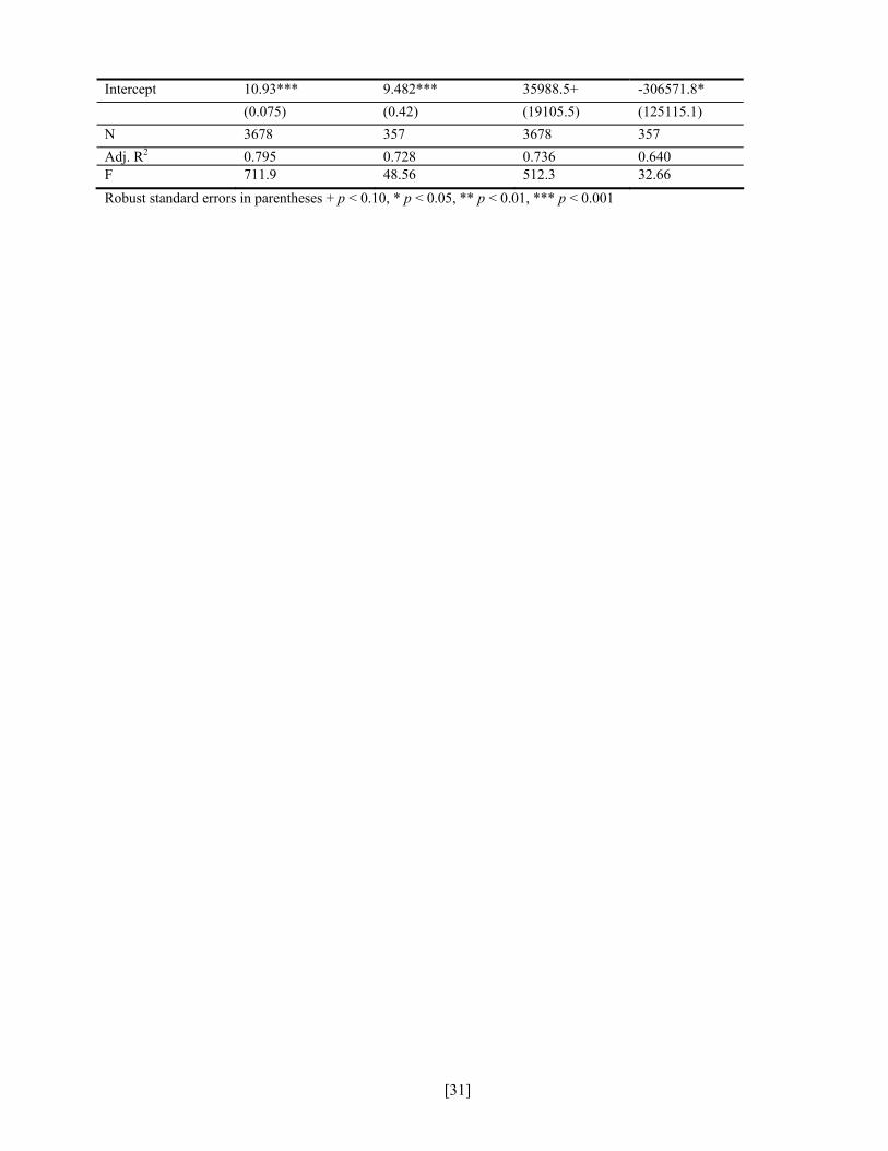
Intercept 10.93*** 9.482*** 35988.5+ -306571.8*

(0.075) (0.42) (19105.5) (125115.1)

N 3678 357 3678 357

Adj. R2 0.795 0.728 0.736 0.640 F 711.9 48.56 512.3 32.66

Robust standard errors in parentheses + p < 0.10, * p < 0.05, ** p < 0.01, *** p < 0.001

[31]

Table 5. Implicit prices for statistically significant parameters*

* N.S. is not significantly different from zero.

Rural Linear Rural Semi Log Urban Linear Urban Semi Log O/GEmp N.S. N.S. $545 $ 571

# Drilling N.S. N.S. - $1,805 - $ 1,354

# Producing N.S. N.S. N.S. $ 289

Dist Drilling N.S. $ 12.21 - $3.71 - $2.62

[32]