Medical Image Segmentation

Xiaolei Huang

Computer Science and Engineering Department, Lehigh University

Gavriil Tsechpenakis

Center for Computational Sciences, University of Miami

Image data is of immense practical importance in medical informatics. Medical images, such as Computed

Axial Tomography (CAT), Magnetic Resonance Imaging (MRI), Ultrasound, and X-Ray, in standard DICOM

formats are often stored in Picture Archiving and Communication Systems (PACS) and linked with other clin-

ical information in EHR clinical management systems. Research efforts havebeen devoted to processing and

analyzing medical images to extract meaningful information such as volume, shape, motion of organs, to detect

abnormalities, and to quantify changes in follow-up studies.

Automated image segmentation, which aims at automated extraction of object boundary features, plays a

fundamental role in understanding image content for searching and mining inmedical image archives. A chal-

lenging problem is to segment regions with boundary insufficiencies, i.e., missing edges and/or lack of texture

contrast between regions of interest (ROIs) and background. To address this problem, several segmentation

approaches have been proposed in the literature, with many of them providing rather promising results.

In this chapter we focus on two general categories of segmentation methodswidely used in medical vision,

namely the deformable models- and the machine learning-based classification approaches. We first review these

two categories of methods and discuss the potential of integrating the two approaches, and then we detail on two

of the most recent methods for medical image segmentation: (i) the Metamorphs,a semi-parametric deformable

model that combines appearance and shape into a unified space, and (ii) the integration of geometric models with

a collaborative formulation of CRFs in a probabilistic segmentation framework.We show different examples

of medical data segmentation, we draw general conclusions from the methods described in this chapter, and we

give future directions for solving challenging and open problems in medicalimage segmentation.

1

Figure 1:(a) Example Dicom header for a CT medical image. (b) Display of one cross-section slice of the CT volume.

1 Introduction

Recent advances in a wide range of medical imaging technologies have revolutionized how we view func-

tional and pathological events in the body and define anatomical structuresin which these events take place.

X-ray, CAT, MRI, Ultrasound, nuclear medicine, among other medical imaging technologies, enable 2D or to-

mographic 3D images to capture in-vivo structural and functional information inside the body for diagnosis,

prognosis, treatment planning and other purposes.

To achieve compatibility and to improve workflow efficiency between imaging systems and other infor-

mation system in healthcare environments worldwide, the Digital Imaging and Communications in Medicine

(DICOM) standard is created as a cooperative international standard for communication of biomedical diagnos-

tic and therapeutic information in disciplines that use digital images and associated data. The DICOM standard,

which includes a file format definition and a network communications protocol, isused in handling, storing,

printing, and transmitting information in medical imaging. Between two entities that arecapable of receiving

image and patient data in DICOM format, DICOM files can be exchanged. An example DICOM file header is

shown in Figure 1(a), and raw image intensities (Figure 1(b)) are stored following the header in the DICOM file.

DICOM also addresses the integration of information produced by variousspecialty applications in the patient’s

Electronic Health Record (EHR). It defines the network and media interchange services allowing storage and

access to these DICOM objects for EHR systems. The National Electrical Manufacturers Association (NEMA)

holds the copyright to the DICOM standard.

Medical images in their raw form are represented by arrays of numbers inthe computer, with the numbers

indicating the values of relevant physical quantities that show contrast between different types of body tissue.

Processing and analysis of medical images are useful in transforming rawimages into a quantifiable symbolic

2

form for ease of searching and mining, in extracting meaningful quantitative information to aid diagnosis, and

in integrating complementary data from multiple imaging modalities.

One fundamental problem in medical image analysis is image segmentation, which identifies the boundaries

of objects such as organs or abnormal regions (e.g. tumors) in images. Having the segmentation result makes it

possible for shape analysis, detecting volume change, and making a precise radiation therapy treatment plan. In

the literature of image processing and computer vision, various theoretical frameworks have been proposed for

segmentation. Among some of the dominant mathematical models are Thresholding [51], region growing [52],

edge detection and grouping [53], Markov Random Fields (MRF) [54],active contour models (or deformable

models) [28], Mumford-Shah functional based frame partition [34], level sets [3, 31], graph cut [24], and mean

shift [9]. Significant extensions and integrations of these frameworks [55, 56, 57, 18, 50, 47, 49] improve their

efficiency, applicability and accuracy.

Despite intensive research, however, segmentation remains a challengingproblem due to the diverse image

content, cluttered objects, occlusion, image noise, non-uniform object texture, and other factors. Particularly,

boundary insufficiencies (i.e. missing edges and/or lack of texture contrast between regions of interest (ROIs)

and background) are common in medical images. In this chapter, we focus on introducing two general categories

of segmentation methods—the deformable models and the learning-based classification approaches—which

incorporate high-level constraints and prior knowledge to address challenges in segmentation. In Section 2,

we aim at giving the reader an intuitive description of the two categories of image segmentation approaches.

We then detail on two specific medical image segmentation methods, theMetamorphsand theCRF Geometric

Models, in Section 3 and Section 4, respectively. We show additional medical image segmentation results in

Section 5, and conclude the chapter in Section 6.

2 Related Work and Further Readings

2.1 Deformable Models for segmentation

Deformable modelsare curves or surfaces that deform under the influence of internal (shape) smoothness and

external image forces to delineate object boundary. Compared to local edge-based methods, deformable models

have the advantage of estimating boundary with smooth curves or surfacesthat bridge over boundary gaps.

The model evolution is usually driven by a global energy minimization process, where the internal and external

energies (corresponding to the smoothness and image forces) are integrated into a model total energy, and the

optimal model position/configuration is the one with the minimum total energy. When initialized far away from

object boundary, however, a model can be trapped in local energy minimacaused by spurious edges and/or

3

(a)

tumor region

A B

C

(b)

Figure 2:Two examples of segmentation using parametric deformable models (active contours). (a) Edge-based modelfor the segmentation of the left and right ventricles (LV,RV) in a cardiac MRI; from left two right: original image, ground-truth boundaries, edge map (Canny edge detection) with the final model solution superimposed (in yellow), ground-truth(red) and final solution (yellow), magnified view of LV and RV along with the ground-truth (red) and the final solution(yellow). (b) Cross-sectional Optical Coherence Tomography (OCT) [20] image showing a tumor in a mouse retina;panel A: original image indicating the tumor inside the box (green dashed line); panel B: five instances (in yellow) of theevolution of a region-based deformable model; panel C: finalsegmentation result (in yellow) for the retinal tumor.TheOCT image is courtesy of S. Jiao, Bascom Palmer Eye Institute, University of Miami.

high noise. Deformable models are divided into two main categories, theparametricand thegeometricmodels.

Among these two classes, there are methods that use edges as image features to drive the model towards the

desired boundaries, and methods that exploit region information for the model evolution.

2.1.1 Parametric Deformable Models

The first class of deformable models is theparametricor explicitdeformable models [28, 8, 33, 48], also known

as active contours, which use parametric curves to represent the modelshape. Edge-based parametric models use

edges as image features, which usually makes them sensitive to noise, while region-based methods use region

information to drive the curve [39, 49, 19]. A limitation of the latter methods is thatthey do not update the region

statistics during the model evolution, and therefore local feature variationsare difficult to be captured. Region

updating is proposed in [13], where active contours with particle filtering isused for vascular segmentation.

Fig. 2 illustrates two examples of medical image segmentation using a parametric deformable model. In the

first example (a), the goal is to segment the left and right ventricle (LV andRV) regions in an MR cardiac image.

The leftmost image shows the original grayscale image, while the second fromleft image shows theground-

4

truth, i.e., the actual boundaries of RV and LV, with two red closed lines; these boundaries were obtained

by manual segmentation. The third (from left) image shows the image edges obtained with the Canny edge

detector; the yellow closed contours superimposed on the edge image show the segmentation result of the

deformable model (initialized around RV and LV), which, in this case, uses edge information as external image

forces [28]. In the next image we show both the ground-truth (in red) and the estimated (in yellow) boundaries.

In the rightmost image, which shows a magnification of the ventricles, one can observe that the deformable

model converges to edges that do not correspond to the actual region boundaries, which is caused by a local

minimum of the model’s energy.

The second example in Fig. 2(b) shows an ultra-high resolution Optical Coherence Tomography (OCT)

[20] cross-sectional image of a mouse retina (panel A): the region insidethe box (green dashed line) is a cross-

section of a retinal tumor, which is the slightly brighter region. In this example, one can understand that the

tumor boundaries are not determined by edges, as in the previous example,but by the texture contrast. Therefore,

the external forces that drive the deformable model are defined by a region-based feature, namely the intensity

distribution: panel B shows five instances of the model evolution, with the circle in the center of the tumor

being the model initialization. Panel C shows the final solution i.e., the configuration/position where the model

converges.

2.1.2 Geometric Models

The second class of deformable models is thegeometricor implicit models [34, 36, 31], which use the level-

set based shape representation, transforming the curves into higher dimensional scalar functions, as shown in

Fig. 3: the1D closed lines of (a) and (c) (evolving fronts) are transformed into the2D surfaces of (b) and

(d) respectively, using the scalar distance function that is mathematically defined in the following sections.

According to this representation, the evolving front corresponds to the cross section of the2D distance function

with the zero level, shown with the gray colored planes in (b) and (d). Moreover, the model interior, i.e., the

region of interest can be implicitly determined by the positive values of the distance surface, as described below.

This distance-based shape representation has two main advantages: (i) the evolving interface can be described

by a single function, even if it consists of more than one closed curves, (ii)the model shape is formulated with a

function of the same dimensionality with the data; that is, for the case of the image segmentation (2D data), the

model shape is also a2D quantity. The latter, and in contrast to using1D parametric curves, enables for more

direct mathematical description of a deformable model.

In [34], the optimal function is the one that best fits the image data, it is piecewise smooth and presents dis-

continuities across the boundaries of different regions. In [36], a variational framework is proposed, integrating

5

(a) (b) (c) (d)

Figure 3:Deformable model shape representation using a distance transform: the shape of the1D closed curves of (a)and (c), that are evolving in the image domain, can be implicitly described by the2D distance functions of (b) and (d)respectively.

boundary and region-based information in PDEs that are implemented using alevel-set approach. These meth-

ods assume piecewise or Gaussian intensity distributions within each partitioned image region, which limits

their ability to capture intensity inhomogeneities and complex intensity distributions.

Fig. 4 illustrates an example of segmentation using a geometric deformable model [43]. The leftmost image

(a) shows anen facefundus image of the human retina obtained with Spectral-Domain Optical Coherence

Tomography (SDOCT) [25]; the bright region in the center of the image is clinically calledGeographic Atrophy

(GA) [42], which corresponds to the atrophy of the retinal pigment epithelium (RPE), common in dry age-

related macular degeneration. Fig. 4(b) shows the result of the GA segmentation (in red); (c) and (d) illustrate

the distance function (colored surface) as shape representation of thedeformable model, for the initialization

and the final configuration of the model respectively. The cross sectionof the surface with the image plane (zero

level) is the evolving boundary. Panel (e) shows eight instances of the deformable model evolution: the red grid

points correspond to the model interior during the evolution (the leftmost image corresponds to the initialization

shown in (c) and the rightmost image shows the final model interior corresponding to (d)).

2.1.3 Edge vs. Region-based Image Features

Although the parametric and geometric deformable models differ in formulation and in implementation, both

traditionally use primarily edge (or image gradient) information to derive external image forces that drive a

shape-based model. In parametric models, a typical formulation [28] for theenergy term deriving the external

image forces is as follows:

Eext(C) = −∫ 1

0

∣

∣∇I(

C(s))∣

∣

2ds (1)

HereC represents the parametric curve model parameterized by curve lengths, I = Gσ ∗ I is the imageI after

smoothing with a Gaussian kernel of standard deviationσ, and∇I(C) is the image gradient along the curve.

Basically by minimizing this energy term, the accumulative image gradient along the curve is maximized, which

6

(a) (b) (c) (d)

(e)

Figure 4: Segmentation of anen facefundus image of the human retina [43], obtained with Spectral-Domain OpticalCoherence Tomography (SDOCT) [25]: the bright region in thecenter is clinically calledGeographic Atrophy(GA)[42], which corresponds to the atrophy of the retinal pigment epithelium (RPE), common in dry age-related maculardegeneration. (a) Originalen faceimage; (b) final position of the deformable model capturing the GA boundaries; (c)-(d)model shape representation of the initialization and the final solution: the cross-section of the surfaces with the imageplane (zero plane) correspond to the model boundary in the image domain; (e) eight instances of the model interior duringthe evolution. The OCT data are courtesy of G. Gregori, B. Lujan, and P.J. Rosenfeld, Bascom Palmer Eye Institute,University of Miami.

means that the parametric model is attracted by strong edges that correspond to pixels with local-maxima image

gradient values.

In geometric models, a typical objective function [3] that drives the frontpropagation of a level set (distance)

function is:

E(C) =

∫ 1

0g(∣

∣∇I(C(s))∣

∣

)∣

∣C′(s)∣

∣ds, where g(∣

∣∇I∣

∣

)

=1

1 +∣

∣∇I∣

∣

2 (2)

Here C represents the front (i.e. zero level set) curve of the evolving level set function. To minimize the

objective function, the front curve deforms along its normal directionC′′(s), and its speed is controlled by the

speed functiong(∣

∣∇I∣

∣

)

. The speed function definition,g(∣

∣∇I∣

∣

)

, depends on image gradient∇I, and it is

positive in homogeneous areas and zero at ideal edges. Hence the curve moves at a velocity proportional to its

curvature in homogeneous regions and stops at strong edges.

The reliance on image gradient information in both parametric and geometric deformable models, however,

makes them sensitive to noise and spurious edges so that the models often need to be initialized close to the

boundary to avoid getting stuck in local minima. Geometric models, in particular, mayleak through boundary

gaps or generate small holes/islands. In order to address the limitations in these deformable models, and develop

more robust models for boundary extraction, there have been significant efforts to integrate region information

into both parametric and geometric deformable models.

7

Along the line of parametric models, region analysis strategies have been proposed [39, 49, 26, 6, 19] to

augment the “snake” (active contour) models. Assuming the partition of an image into an object region and

a background region, a region-based energy criterion for active contours is introduced in [39], which includes

photometric energy terms defined on the two regions. In [49], a generalized energy function that combines

aspects of snakes/balloons and region growing is proposed and the minimization of the criterion is guaranteed

to converge to a local minimum. This formulation still does not address the problem of unifying shape and ap-

pearance however, because of the large difference in representation for shape and appearance. While the model

shape is represented using a parametric spline curve, the region intensity statistics are captured by parameters of

a Gaussian distribution. This representation difference prevents the useof gradient descent methods to update

both region parameters and shape parameters in a unified optimization process, so that the two sets of parame-

ters are estimated in separate steps in [49] and the overall energy functionis minimized in an iterative way. In

other hybrid segmentation frameworks [6, 26], a region based module is used to get a rough binary mask of the

object of interest. Then this rough boundary estimation serves as initializationfor a deformable model, which

will deform to fit edge features in the image using gradient information.

Along the line of geometric models, the integration of region and edge information[50, 40, 47, 36] has been

mostly based on solving reduced cases of the minimal partition problem in the Mumford and Shah model for seg-

mentation [34]. In the Mumford-Shah model, an optimal piecewise smooth function is pursued to approximate

an observed image, such that the function varies smoothly within each region, and rapidly or discontinuously

across the boundaries of different regions. The solution representsa partition of the image into several regions.

A typical formulation of the framework is as follows:

FMS(u, C) =

∫

Ω(u − u0)

2dxdy + a

∫

Ω\C|∇u|2dxdy + b|C| (3)

Hereu0 is the observed, possibly noisy image, andu is the pursued “optimal” piecewise smooth approximation

of u0. Ω represents the image domain,∇u is the gradient ofu, andC are the boundary curves that approximate

the edges inu0. One can see that the first term of the function minimizes the difference betweenu andu0, the

second term pursues the smoothness within each region (i.e. outside the setC), and the third term constraints

the boundary curvesC to be smooth and have the shortest distance.

Although the above framework nicely incorporates gradient and region criteria into a single energy function,

no practical globally-optimal solution for the function is available, most notablybecause of the mathematical

difficulties documented e.g. in [34]. In the recent few years, progresshas been made and solutions for several

reduced cases of the Mumford-Shah functional have been proposedin the level set framework. One approach

8

in [50] is able to segment images that consist of several regions, each characterizable by a given statistics such

as the mean intensity and variance. Nevertheless the algorithm requires known a priori the number of segments

in the image and its performance depends upon the discriminating power of the chosen set of statistics. Another

approach in [40] applies a multi-phase level set representation to segmentation assuming piece-wise constant

intensity within one region. It is considered as solving a classification problem because it assumes the mean

intensities of all region classes are knowna priori, and only the set of boundaries between regions is unknown.

In the works presented by [4, 47], piece-wise constant and piece-wise smooth approximations of the Mumford-

Shah functional are derived for two-phase (i.e. two regions) [4] or multiphase (i.e. multiple regions) [47] cases

in a variational level set framework. The optimization of the framework is based on an iterative algorithm that

approximates the region mean intensities and level-set shape in separate steps. Geodesic Active Region[36] is

another method that integrates edge and region based modules in a level setframework. The algorithm consists

of two stages: a modeling stage that constructs a likelihood map of edge pixels and approximates region/class

statistics using Mixture-of-Gaussian components, and a segmentation stage that uses level set techniques to

solve for a set of smooth curves that are attracted to edge pixels and partition regions that have the expected

properties of the associated classes. In summary of the above approaches, they all solve the frame partition

problem, which can be computationally expensive when dealing with busy images that contain many objects

and clutter. Their assumptions of piece-wise constant, piece-wise smooth, Gaussian, or Mixture-of-Gaussian

intensity distributions within regions can also limit their effectiveness in segmenting objects whose interiors

have textured appearance and/or complex multi-modal intensity distributions.

2.2 Learning-based classification for segmentation

Learning-based pixel and region classificationis among the popular approaches for image segmentation. This

kind of methods exploit the advantages of supervised learning (training from examples) to assign probabilities

of belonging to the region of interest to image sites. Graphical models are commonly used to incorporate neigh-

borhood interactions and contextual information, and they can be characterized as eithergenerativeor discrim-

inative. Generative models are commonly used in segmentation/recognition problems where the neighboring

property is well defined among the data, and they are robust to compositionality (variations in the input features),

without having to see all possibilities during training. However, generativemodels can be computationally in-

tractable since they require representations of multiple interacting features or long-range dependencies. On

the other hand, discriminative models, such as Support Vector Machines (SVMs) and logistic regression, infer

model parameters from training data and directly calculate the class posteriorgiven the data (mapping); they

are usually very fast at making predictions, since they adjust the resultingclassification boundary or function

9

approximation accuracy, without the intermediate goal of forming ageneratorthat models the underlying distri-

butions during testing. However, discriminative models often need large training sets in order to make accurate

predictions, and therefore they cannot be used for data with relatively high rates of ambiguities in a straightfor-

ward way. To address this problem, some approaches integrate discriminative with generative models, where

the parameters of a generative approach are modeled and trained in a discriminative manner. Also, for the same

purpose, discriminative methods are used in active learning frameworks,to select the most descriptive examples

for labeling, in order to minimize the model’s entropy without increasing the size of the training set.

2.2.1 Markov Random Fields (MRFs)

A representative example of learning-based region classification is the Markov Random Fields (MRFs) [16].

According to MRFs, the image is divided intosites, either at the pixel level or at the level of patches of pre-

determined spatial scale (size). Each site corresponds to: (i) a hidden node, or label node, which is the desired

label to be calculated for the specific site: in region segmentation, this label can be eitherregion of interest

or background, and (ii) the observation, or feature node, which corresponds to the site’s feature set directly

estimated from the image.

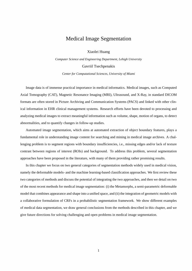
Fig. 5 illustrates the idea of learning-based classification of image sites using acommon MRF. Panel (a)

shows the original image of the example of Fig. 2(b) , and panel (b) showsin magnification the region indicated

by the yellow box in (a). The yellow patches in (b) indicate the sites, which, in this case, correspond to single

pixels. Fig. 5(c) shows the graphical representation of the MRF. The upper level is the label field to be calcu-

lated, where each node corresponds to the (unknown) label of each pixel. The lower level is the observation set,

where each node (usually indicated with a box) corresponds to the feature vector of each site; here, the feature

vector contains a single value, which is the grayscale value of the pixel. Specifically in MRFs, the label of each

site depends on (i) the corresponding observation and (ii) the labels of its neighboring sites; we illustrate these

dependencies with the solid and dashed lines. The segmentation result is obtained as a global optimization prob-

lem, i.e., estimating the optimal label field, given the observations. In contrast totraditional deformable models

that follow deterministic energy minimization approaches, learning-based classification methods are usually

based on a probabilistic solution, i.e., they are driven by the maximization of a probability. Fig. 5(d) illustrates

the probabilities of all pixels belonging to the region of interest, i.e., the tumor: bright regions correspond to

high probabilities, while darker regions denote the least likely sites to belong tothe tumor. The label field of the

image (tumor vs. background) is derived by thresholding these probabilityvalues.

10

Label field

Observations

(a) (b) (c) (d)

Figure 5: Image segmentation for the example of Fig. 2(b): probability field estimated by a MRF. Panel (b) showsa magnification of the region inside the yellow box in (a): theyellow grid shows the image sites, which in this casecorrespond to pixels. Panel (c) shows the graphical representation of the MRF, where each feature (gray box) correspondsto the intensity value of a pixel. Panel (d) shows the probability field for the entire image: the bright regions indicate highprobability of belonging to the ROI (tumor); by thresholding these probabilities we obtain the ROI.

2.2.2 Conditional Random Fields (CRFs)

Intuitively, the common MRF formulation assumes that neighboring image sites should have similar labels,

and this (markovian) property results to smooth probability fields. To obtain better probability smoothing,

Conditional Random Fields (CRFs) were introduced in computer vision by Laffert et al. [30]. Although CRFs

were first used to label sequential data, extensions of them are used for image segmentation [29, 15, 46, 45,

43, 44]. The main advantage of CRFs is that they handle the known label bias problem [30], avoiding the

conditional independence assumption among the features of neighboring sites (the labels neighboring property

is driven by the corresponding features). In [29] the Discriminative Random Fields (DRFs) are presented, which

allow for computationally efficient MAP inference. Also, in [15], CRFs areused in different spatial scales to

capture the dependencies between image regions of multiple sizes. A potentiallimitation of CRFs is that they

do not provide robustness to unobserved or partially observed features, which is a common problem in most

discriminative learning models.

2.3 Integration of Deformable Models with Learning-based Classification

The integration of deformable models with learning-based classification is a recently introduced framework for

propagating deformable models in a probabilistic manner, by formulating thetraditional energy minimization

as amaximum a posteriori probability(MAP) estimation problem. The main advantages of such integration

are: (i) the model evolution provides a framework for updating the region statistics in a learning-based region

classification, (b) the probabilistic formulation can provide the desired robustness to data (region) ambiguities,

and (c) the final solution is a locally smooth boundary around the region of interest, due to the deformable model

formulation. In the survey of [33], methods that use probabilistic formulations are described. In the work of [19]

11

the integration of probabilistic active contours with MRFs in a graphical framework is proposed to overcome the

limitations of edge-based probabilistic active contours. In [16], a framework that tightly couples 3D MRFs with

deformable models is proposed for the 3D segmentation of medical images. To exploit the superiority of CRFs

compared to common first-order MRFs, a coupling framework is proposed in[46, 44], where a CRF and an

implicit deformable model are integrated in a simple graphical model. More recently, in [43, 45] the integration

of geometric models with CRFs were used for medical image segmentation.

3 The Metamorphs Model

In this section, we describe a new class of deformable models, termed “Metamorphs”, which integrates edge-

and region-based image features for robust image segmentation. A Metamorphs model does not requirea

priori off-line learning, yet enjoys the benefit of having appearance constraints by online adaptive learning of

model-interior region intensity statistics. The basic framework of applying a Metamorphs model to boundary

extraction is depicted in Fig. 6. The object of interest in this example is the corpus callosum structure in an

MRI image of the brain. First, a simple-shape (e.g. circular) model is initialized inside the corpus callosum

(see the blue circle in Fig. 6(a)). Considering the model as a “disk”, it hasa shape and covers an area of the

image which is the interior of the current model. The model then deforms towardedges as well as toward the

boundary of a region that has similar intensity statistics as the model interior. Fig. 6(b) shows the edges detected

using a canny edge detector; note that the edge detector with automatically-determined thresholds gives a result

that has spurious edges and boundary gaps. To counter the effect of noise in edge detection, we estimate a

region of interest (ROI) that has similar intensity statistics with the model interior.To find this region, we first

estimate the model-interior probability density function (p.d.f.) of intensity, then a likelihood map is computed

which specifies the likelihood of a pixel’s intensity according to the model-interior p.d.f. Fig. 6(c) shows the

likelihood map computed based on the initial model interior; and we threshold the likelihood map to get the

ROI. The evolution of the model is then derived using a gradient descentmethod from a unified variational

framework that consists of energy terms defined on edges, the ROI boundary, and the likelihood map. Fig. 6(d)

shows the model after 15 iterations of deformation. As the model deforms, themodel interior and its intensity

statistics change, and the new statistics lead to the update of the likelihood map andthe update of the ROI

boundary for the model to deform toward. This online adaptive learning process empowers the model to find

the boundary of objects with non-uniform appearance more robustly. Fig. 6(e) shows the updated likelihood

map given the evolved model in Fig. 6(d). Finally, the model converges taking a balance between the edge and

region influences, and the result is shown in Fig. 6(f).

12

(a) (b) (c) (d) (e) (f)

Figure 6: Metamorphs segmentation of a brain structure. (a) An MRI image of the brain; the initial circular model isdrawn on top. (b) Edges detected using canny edge detector. (c) The intensity likelihood map computed according to theintensity probability density function of the initial model interior. (d) Intermediate evolving model after 15 iterations. (e)The intensity likelihood map according to the intermediatemodel’s interior statistics. (f) Final converged model after 38iterations.

The key property of Metamorphs is that these new models have both shape and appearance, and they nat-

urally integrate edge information with region statistics when applied to segmentation. By doing so, these new

models generalize the two major classes of deformable models in the literature, namely theparametricmod-

els and thegeometricmodels, which are traditionally shape-based, and take into account only edge or image

gradient information.

3.1 The Metamorphs Shape Representation

The model’s shape is embedded implicitly in a higher dimensional space of distance transforms. The Euclidean

distance transform is used to embed the boundary of an evolving model as the zero level set of a higher dimen-

sional distance function [35]. In order to facilitate notation, we consider the 2D case. LetΦ : Ω → R+ be

a Lipschitz function that refers to the distance transform for the model shapeM. By definitionΩ is bounded

since it refers to the image domain. The shape defines a partition of the domain: the region that is enclosed by

M, [RM], the background [Ω−RM], and on the model, [∂RM] (a very narrow band around the model shape

M). Given these definitions the following implicit shape representation forM is considered:

ΦM(x) =

0, x ∈ ∂RM

+D(x,M), x ∈ RM

−D(x,M), x ∈ [Ω −RM]

(4)

whereD(x,M) refers to the minimum Euclidean distance between the image pixel locationx = (x, y) and the

modelM.

Such implicit embedding makes the model shape representation a distance map “image”, which greatly fa-

cilitates the integration of shape and appearance information. It also provides a feature space in which objective

functions that are optimized using a gradient descent method can be conveniently used. A sufficient condition

for convergence of gradient descent methods requires continuous first derivatives, and the considered implicit

13

(1)

(2)(a) (b) (c)

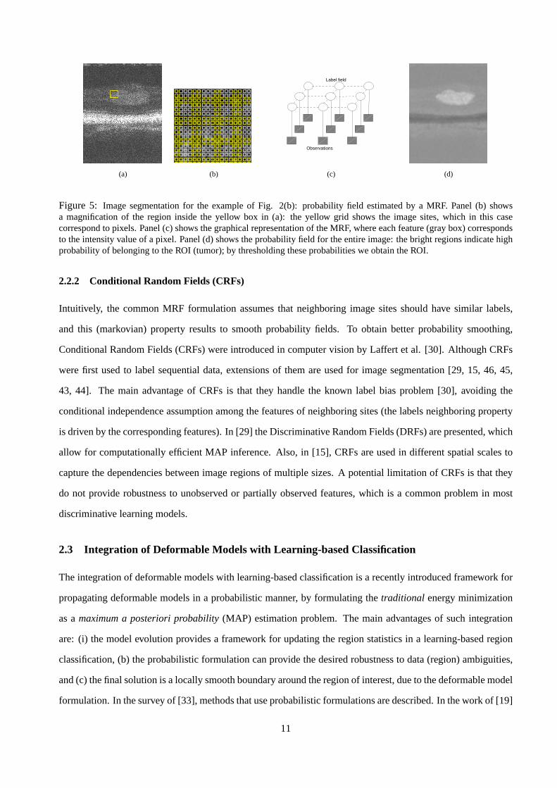
Figure 7:Shape representation and deformations of Metamorphs models. (1) The model shape. (2) The implicit distancemap “image” representation of the model shape. (a) Initial model. (b) Example FFD control lattice deformation to expandthe model. (c) Another example of the free-form model deformation given the control lattice deformation.

representation satisfies this condition. In fact, one can prove that the gradient of the distance function is a unit

vector in the normal direction of the shape. This property will make our modelevolution fast. Examples of the

implicit representation can be found in Figs. 3 and 4(c)-(d).

3.2 The Model’s Deformations

The deformations that a Metamorphs model can undergo are defined usinga space warping technique, the Free

Form Deformations (FFD) [41, 12], which is a popular approach in graphics and animation. The essence of

FFD is to deform the shape of an object by manipulating a regular control lattice F overlaid on its volumetric

embedding space. The deformation of the control lattice consists of displacements of all the control points in the

lattice, and from these sparse displacements, a dense deformation field forevery pixel in the embedding space

can be acquired through interpolation using interpolating basis functions such as the Cubic B-spline functions.

One illustrative example is shown in Fig. 7. A circular shape [Fig. 7(1.a)] is implicitly embedded as the zero

level set of a distance function [Fig. 7(1.b)]. A regular control lattice is overlaid on this embedding space. When

the embedding space deforms due to the deformation of the FFD control lattice as shown in Fig. 7(b), the shape

undergoes an expansion. Fig. 7(c) shows another example of free-form shape deformation given a particular

FFD control lattice deformation. In Metamorphs, we consider an Incremental Free Form Deformations (IFFD)

formulation using the cubic B-spline basis functions for interpolation [17].

Compared with optical-flow type of deformation representation (i.e. pixel-wisedisplacements inx andy

directions) commonly used in the literature, the IFFD parameterization we use allows faster model evolution and

convergence, because it has significantly fewer parameters. A hierarchical multi-level implementation of IFFD

[17], which uses multi-resolution control lattices according to a coarse-to-fine strategy, can account for defor-

14

mations of both large and small scales. The advantages of coarse-to-fineoptimization have been demonstrated

in deformable contour frameworks in the literature [1]. Another property of IFFD is that it imposes implicit

smoothness constraints, since it guaranteesC1 continuity at control points andC2 continuity everywhere else.

Therefore there is no need to introduce computationally-expensive regularization components on the deformed

shapes. As a space warping technique, IFFD also integrates naturally withthe implicit shape representation

which embeds the model shape in a higher dimensional space.

3.3 The Model’s Texture

To approximate the intensity distribution of the model interior, we model the distribution using a nonparametric

kernel-based density estimation method, also known as the Parzen windows technique [10], which is a popular

nonparametric statistical method. Recently this technique has been applied to imaging and computer vision,

most notably in modeling the varying background in video sequences [11],and in approximating multi-modal

intensity density functions of color images [9]. Here, we use this representation to approximate the intensity

probability density function (p.d.f.) of the model interior.

Suppose the model is placed on an imageI, the image region bounded by current modelΦM is RM,

then the intensity p.d.f. of the model interior region can be represented usinga Gaussian kernel-based density

estimation:

P(i∣

∣ΦM) =1

V (RM)

∫∫

RM

1√2πσ

e−(i−I(y))2

2σ2 dy (5)

wherei = 0, ..., 255 denotes the pixel intensity values,V (RM) denotes the volume ofRM, y represents pixels

in the regionRM, andσ is a constant specifying the width of the Gaussian kernel.

One example of this nonparametric density estimation can be seen in Fig. 8. The zero level set of the

evolving modelsΦM are drawn on top of the original image in Fig. 8(a). The model interior regionsRM are

cropped and shown in Fig. 8(b). Given the model interiors, their nonparametric intensity p.d.f.sP(i∣

∣ΦM) are

shown in Fig. 8(c), where the horizontal axis denotes the intensity valuesi = 0, ..., 255, and the vertical axis

denotes the probability valuesP ∈ [0, 1]. Finally, over the entire imageI, we evaluate the probability of every

pixel’s intensity, according to the model interior intensity p.d.f., and the resultingprobability (or likelihood)

map is shown in Fig. 8(d).

Using this nonparametric estimation, the intensity distribution of the model interior gets updated automat-

ically while the model deforms to cover a new set of interior pixels; and it avoids having to estimate and keep

a separate set of intensity parameters such as the mean and variance if a Gaussian or Mixture-of-Gaussian

15

(1) 0 50 100 150 200 2500

0.05

0.1

0.15

0.2

0.25

0.3

(2) 0 50 100 150 200 2500

0.05

0.1

0.15

0.2

0.25

0.3

(3) 0 50 100 150 200 2500

0.05

0.1

0.15

0.2

0.25

0.3

(a) (b) (c) (d)

Figure 8: Left Ventricle endocardium segmentation, demonstrating Metamorphs appearance representation. (1) Initialmodel. (2) Intermediate result after 4 iterations. (3) Final converged result after 10 iterations. (a) The evolving modeldrawn on original image. (b) Interior region of the evolvingmodel. (c) The intensity p.d.f. of the model interior. (d) Theimage intensity probability map according to the p.d.f. of the model interior.

model was used. Moreover, this kernel-based estimation in Eq. 5 is a continuous function, which facilitates the

computation of derivatives in a gradient-descent based optimization framework.

3.4 The Metamorphs’ Dynamics

In order to fit to the boundary of an object, the motion of the model is driven by two types of energy terms

derived from the image: the edge data termsEE , and the region data termsER. So the overall energy functional

E is defined by [18]:

E = EE + kER (6)

wherek is a constant balancing the contributions from the two types of terms. In this formulation, we are able

to omit the model smoothness term, since this smoothness is implicit by using Free Form Deformations.

3.4.1 The edge termEE

The Metamorphs model is attracted to edge features with high image gradient. Weencode the edge information

using a “shape image”Φ, which is the un-signed distance transform of the edge map of the image. Theedge

map is computed using Canny Edge Detector with default parameter settings. InFig. 9(c), we can see the “shape

image” of an example MR heart image.

Intuitively, this edge term encourages deformations that map the model boundary pixels to image locations

16

(a) (b) (c)

Figure 9: Effects of small spurious edges on the “shape image”. (a) An MRI image of the heart; the interested objectboundary is the endocardium of the left ventricle. (b) Edge map of the image. (c) The derived “shape image” (distancetransform of the edge map), with edges drawn on top. Note how the small spurious edges affect the “shape image” valuesinside the object.

7 8 8 8 8 8 9 9 8 8 7 7 6 6 5 5 4 4 3 2 1 1 0 1 2 3 2 1 0 1 28 8 9 9 9 9 9 109 9 8 8 7 7 6 6 5 4 4 3 2 1 0 1 2 3 2 1 0 1 19 9 101010101011109 9 9 8 8 7 6 5 4 4 3 2 1 0 1 2 3 2 1 1 0 19 101111111111111110109 8 7 6 5 4 4 3 2 1 1 0 1 2 3 3 2 1 0 1101111121212121111109 9 8 7 6 5 4 3 2 1 1 0 1 1 2 3 3 2 1 0 11112121313121111109 9 8 8 7 6 5 4 3 2 1 0 1 1 2 3 4 3 2 1 0 112131313121111109 8 8 7 7 6 6 5 4 3 2 1 0 1 2 3 4 4 3 2 1 0 1131313121111109 8 8 7 6 6 5 5 5 4 3 2 1 0 1 1 2 3 4 3 2 1 0 11413131211109 8 8 7 6 6 5 4 4 4 4 3 2 1 1 0 1 2 3 4 3 2 1 0 114131211109 9 8 7 6 6 5 4 4 3 3 3 3 3 2 1 0 1 2 3 4 3 2 1 0 114131211109 8 7 6 6 5 4 4 3 2 2 2 2 3 2 1 0 1 2 3 4 3 2 1 1 0131211109 9 8 7 6 5 4 4 3 2 1 1 1 1 2 2 1 1 1 2 3 4 4 3 2 1 0131211109 8 7 6 5 4 4 3 2 1 1 0 0 1 2 3 2 2 2 3 4 4 4 3 2 1 0131211109 8 7 6 5 4 3 2 1 1 0 1 1 1 2 3 3 3 3 4 4 4 4 3 2 1 0131211109 8 7 6 5 4 3 2 1 0 1 1 2 2 3 4 4 4 4 4 5 4 3 2 1 1 0121111109 8 7 6 5 4 3 2 1 0 1 2 3 3 4 4 5 5 5 5 5 4 3 2 1 0 11211109 8 8 7 6 5 4 3 2 1 0 1 2 3 4 4 5 6 6 6 6 5 4 3 2 1 0 111109 9 8 7 6 5 4 4 3 2 1 0 1 2 3 4 5 6 6 7 7 6 5 4 3 2 1 0 111109 8 7 6 6 5 4 3 2 1 1 0 1 2 3 4 5 6 7 7 6 5 4 4 3 2 1 0 1109 8 8 7 6 5 4 4 3 2 1 0 1 1 2 3 4 5 6 7 7 6 5 4 3 2 1 1 0 19 8 8 7 6 5 4 4 3 2 1 1 0 1 2 3 4 4 5 6 7 6 5 4 4 3 2 1 0 1 18 8 7 6 6 5 4 3 2 1 1 0 1 1 2 3 4 5 6 7 6 6 5 4 3 2 1 1 0 1 27 7 6 6 5 4 4 3 2 1 0 1 1 2 3 4 4 5 6 7 6 5 4 4 3 2 1 0 1 1 26 6 5 5 4 4 3 2 1 1 0 1 2 3 4 4 5 6 7 6 5 4 4 3 2 1 1 0 1 2 35 5 4 4 4 3 2 1 1 0 1 1 2 3 4 5 6 6 6 6 5 4 3 2 1 1 0 1 1 2 34 4 4 3 3 2 1 1 0 1 1 2 3 4 4 5 6 6 6 5 4 4 3 2 1 0 1 1 2 3 43 4 3 2 2 1 1 0 1 1 2 3 4 4 5 6 6 6 5 4 4 3 2 1 1 0 1 2 3 4 42 3 2 1 1 1 0 1 1 2 3 4 4 5 6 6 6 5 4 4 3 2 1 1 0 1 1 2 3 4 51 2 1 1 0 0 1 1 2 3 4 4 5 6 6 5 5 4 4 3 2 1 1 0 1 1 2 3 4 4 51 2 1 0 1 1 1 2 3 4 4 5 6 6 5 4 4 4 3 2 1 1 0 1 1 2 3 4 4 4 41 1 1 0 1 2 2 3 4 4 5 6 5 5 4 4 3 3 2 1 1 0 1 1 2 3 4 3 3 3 3

(a) (b) (c) (d)

Figure 10:At a small gap in the edges, the edge data term constraints themodel to go along a path that coincides with thesmooth shortest path connecting the two open ends of the gap.(a) Original Image. (b) The edge map, note the small gapinside the square. (c) The “shape image”. (d) Zoom-in view ofthe region inside the square. The numbers are the “shapeimage” values at each pixel location. The red dots are edge points, the small blue squares indicate a path favored by theedge term for a Metamorphs model.

closer to edges, so that the underlying “shape image” values are as small (or as close to zero) as possible.

During optimization, this term will deform the model along the gradient direction of the underlying “shape

image” toward edges. Thus it will expand or shrink the model accordingly,serving as a two-way balloon force

implicitly and making the attraction range of the model large.

One additional advantage of this edge term is that, at an edge with small gaps,this term will constrain the

model to go along the “geodesic” path on the “shape image”, which coincideswith the smooth shortest path

connecting the two open ends of a gap. This behavior can be seen from Fig. 10. Note that at a small gap on an

edge, the edge term favors a path with the smallest accumulative distance values to the edge points.

3.4.2 The Region Data TermER

An attractive aspect of the Metamorphs is that their interior intensity statistics are learned dynamically, and

their deformations are influenced by forces derived from this dynamically-changing region information. This

region information is very important in helping the models out of local minima, and converge to the true object

boundary. In Fig. 9, the spurious edges both inside and around the object boundary degrade the reliability of

17

(1)

(2) 0 50 100 150 200 2500

0.1

0.2

0.3

0.4

0.5

0.6

0.7

0.8

0.9

1

(3) 0 50 100 150 200 2500

0.1

0.2

0.3

0.4

0.5

0.6

0.7

0.8

0.9

1

(4) 0 50 100 150 200 2500

0.1

0.2

0.3

0.4

0.5

0.6

0.7

0.8

0.9

1

(a) (b) (c) (d)

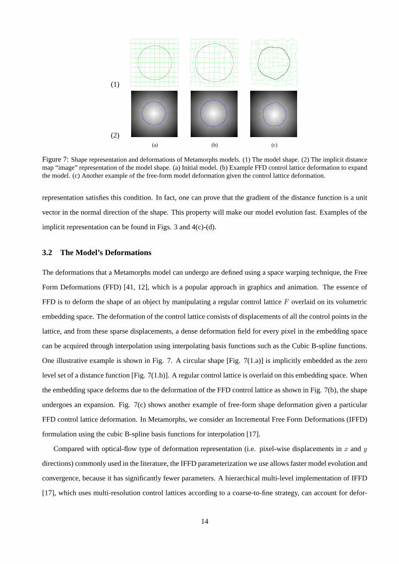
Figure 11:Segmentation of the Left Ventricle endocardium in an MRI image. (1.a) the original image. (1.b) the edgemap; note that a large portion of the object boundary is missing in the edge map. (1.c) the “shape image”. (2) initialmodel. (3) intermediate model. (4) converged model. (a) zero level set of the current model drawn on the image. (b)model interiors. (c) the interior intensity p.d.f.s. (d) intensity probability maps.

the “shape image” and the edge data term. Yet the intensity probability maps computed based on model-interior

intensity statistics, as shown in Fig. 8(d), give a consistent and clear indication on where the rough boundary

of the object is. In another MR heart image shown in Fig. 11(1.a), a large portion of the object boundary

(LV endocardium) is missing during computation of the edge map using default canny edge detector settings

[Fig. 11(1.b)]. Relying solely on the “shape image” [Fig. 11(1.c)] and theedge data term, a model would

have leaked through the large gap and mistakenly converged to the outer epicardium boundary. In this situation,

the probability maps [Fig. 11(2-4.d)] computed based on model-interior intensity statistics become the key to

optimal model convergence.

In our framework, we define two region data terms – a “Region Of Interest”(ROI) based balloon termERl

and a Maximum Likelihood termERm, so the overall region-based energy functionER is:

ER = ERl+ bERm

(7)

The ROI based Balloon TermERl. We determine the “Region Of Interest” (ROI) as the largest possible

18

(a) (b) (c)

Figure 12: Deriving the ROI based region data term. (a) The model shown on the original image. (b) The intensityprobability map computed based on the model interior statistics. (c) The “shape image” encoding boundary informationof the ROI.

region in the image that overlaps the model and has a consistent intensity distribution as the current model

interior. The ROI-based balloon term is designed to efficiently evolve the model toward the boundary of the

ROI.

Given a modelM on imageI [Fig. 12(a)], we first compute the image intensity probability mapPI [Fig.

12(b)], based on the model interior intensity statistics (see Eq. 5 in section 3.3). A threshold (typically the mean

probability over the entire image domain) is applied onPI to produce a binary imagePB. More specifically,

those pixels that have probabilities higher than the threshold inPI are given the value1 in PB, and all other

pixels are set to the value0 in PB. We then apply a connected component analysis algorithm based on run-length

encoding and scanning [21] onPB to extract the connected component that overlaps the model. Considering

this connected component as a “disk” that we want the Metamorphs model to match, it is likely that this disk

has small holes due to noise and intensity inhomogeneity, as well as large holesthat correspond to real “holes”

inside the object. How to deal with compound objects that potentially have holes using Metamorphs is an

interesting question that we will discuss briefly in Section 6. Here, we assumethe regions of interest that we

apply Metamorphs to segment are without interior holes. Under this assumption, the desired behavior of the

model is to evolve toward the ROI border regardless of small holes in the ROIconnected component. Hence

we take the outer-most border of the selected connected component as thecurrent ROI boundary. We encode

this ROI boundary information by computing its “shape image”, which is its un-signed distance transform [Fig.

12(c)].

Within the overall energy minimization framework, the ROI-based balloon term is the most effective in

countering the effect of un-regularized or inhomogeneous region intensities such as that caused by speckle

noise and spurious edges inside the object of interest (e.g. in Fig. 9 and Fig. 13). This is because the ROI term

deforms the model toward the outer-most boundary of the identified ROI, disregarding all small holes inside.

Although this makes the assumption that the object to be segmented has no holes,it is a very effective measure

to discard incoherent pixels and make noise and intensity inhomogeneity not toinfluence model convergence.

19

(1)

(2) 0 50 100 150 200 2500

0.05

0.1

0.15

0.2

0.25

0.3

(3) 0 50 100 150 200 2500

0.05

0.1

0.15

0.2

0.25

0.3

(4) 0 50 100 150 200 2500

0.05

0.1

0.15

0.2

0.25

0.3

(a) (b) (c) (d)

Figure 13:Tagged MRI heart image example. (1.a) Original image. (1.b)Edge map. (1.c) “shape image” derived fromthe edge map. (2) Initial model. (3) Intermediate result. (4) Converged model (after 12 iterations). (2-4)(a) The evolvingmodel. (2-4)(b) Model interior. (2-4)(c) Model interior intensity p.d.f. (2-4)(d) Intensity probability map according to thep.d.f. in (c).

Moreover, the ROI term generates adaptively changing balloon forcesthat expedite model convergence and

improve convergence accuracy, especially when the object shape is elongated, or has salient protrusions or

concavities.

The Maximum Likelihood Term ERmThe previous ROI term is efficient in deforming the model toward

object boundary when the model is still far away. When the model gets closeto the boundary, however, the ROI

may become less reliable due to intensity changes in the boundary areas. To achieve better convergence, we

design another Maximum Likelihood (ML) region-based data term that constrains the model to deform toward

areas where the pixel intensity probabilities of belonging to the model-interior intensity distribution are high.

This ML term is formulated by maximizing the log-likelihood of pixel intensities in a narrow band around the

model [18]. During model evolution, when the model is still far away from theobject boundary, this ML term

generates very little force to influence the model deformation. When the modelgets close to the boundary, the

ML term helps the model to converge and is particularly useful in preventingthe model from leaking through

large gaps (e.g. in Fig. 11).

20

4 The CRF-driven Geometric Model

In this section, we describe Conditional Random Field-driven Geometric Model, a method that integrates de-

formable models with learning-based classification.

A topology independent solution is presented for segmenting regions of interest with texture patterns of any

scale, using an implicit deformable model driven by Conditional Random Fields (CRFs). This model integrates

region and edge information as image driven terms, whereas the probabilisticshape and internal (smoothness)

terms use representations similar to the level-set based methods. The evolutionof the model is solved as a

maximum a posteriori probability(MAP) estimation problem, where the target conditional probability is de-

composed into the internal term and the image-driven term. For the later, we use discriminative CRFs in two

scales, pixel- and patch-based, to obtain smooth probability fields based onthe corresponding image features.

In this method, (i) we use the shape representation of known level-set based approaches, to achieve topology

independence, (ii) we integrate edge and region information, which is beingupdated during the model evolution,

to handle local feature variations, (iii) we avoid the problem of getting trapped in local minima, which most of

the energy minimization driven models suffer from, (iv) we exploit the superiority of CRFs compared to MRFs

for image segmentation, coupling a CRF-based scheme with the deformable model,and (v) we capture higher

scale dependencies, using pixel- and patch-based CRFs. We use the two-scale CRF model in a tightly coupled

framework with the deformable model, such that the external (image-driven) term of the deformable model

eventually corresponds to the smooth probability field estimated by the CRF. We use a modified version of

the discriminative CRFs presented in [29], where the MAP inference is computationally tractable using graph

min-cut algorithms.

4.1 Deformable Model Shape and Energy

In a similar way as in Metamorphs (see 3.1, eq. (4)), the model’s shape is embedded in a higher dimensional

space of distance transforms, such that the zero-level of the scalar (Euclidean distance) functionΦM corresponds

to the evolving front. The modelM (interface) defines two regions in the image domainΩ, namely the region

RM enclosed by the modelM and the background[Ω −RM].

The internal energy of the model consists of three individual terms, namelythe smoothness constraint

Esmooth, the distance from the target shapeEshape, and a partitioning energy termEpart,

Eint(ΦM) = Esmooth(ΦM) + Epart(ΦM) + Eshape(ΦM) (8)

21

The smoothness termEsmooth. We define the energy term that enforces smoothness along the model

boundary as,

Esmooth(ΦM) = ε1A(RM) + ε2

∫ ∫

∂RM

‖∇ΦM(x)‖dx (9)

whereε1 andε2 are weighting constants,∂RM denotes a narrow band around the model boundary, andA(RM)

denotes the area of the model interiorRM. The minimization of this energy forces the model to the position

with the minimum area enclosed and the maximum first-order smoothness along the model boundary;∇ΦM

is defined on∀x ∈ Ω, and is used similarly as in the Mumford-Shah formulation [34], i.e., determines the 1st

order smoothness along the boundary.

The partitioning energy Epart. The partitioning energyEpart(ΦM) [43] forces the regionΦM ≥ 0

(model interior, including the pixels on the interface) towards a connected form. It can be also seen as a term

that minimizes the entropy of a set of particles, where the particles are assumed to be the connected components

of ΦM ≥ 0. The minimization of this energy forces the model towards the minimum distances between the

connected components (interior particles), i.e., forces different regions (curves) on the image plane to merge.

Fig. 4 illustrates an example of the effect of this energy term: the model is initialized in three different positions

on the image plane, and during the evolution, the model is forced towards a connected form. Intuitively, merging

different regions (model interior) competes the data driven terms, and therefore, sometimes the image features

do not allow for this merging.

The shape-based energyEshape. The role of the shape-based energy term is to force the evolving model

towards a desired shape, in cases where we have a prior knowledge about the ROI in terms of its shape. This

is a common approach in medical image analysis, since in many applications the goal is to segment ROIs with

specific anatomic features. Introducing this term in the model energy, we combine the bottom-up approach (use

image features to find a region) with a top-down methodology (use prior knowledge about the ROI to detect it

in an image). This shape-based term is defined in a similar way as in [37, 5], interms of the distance between

the model and the target shape.

4.2 The Model Dynamics

According to the CRF-driven geometric model, the goal is to find the optimal model position on the image

plane, as well as the optimal probability field of all pixels/regions. Therefore, we formulate the deformable

model evolution as a joint maximum a posteriori probability (MAP) estimation problem for the model position

and the image label field,

〈Φ∗M,L∗〉 = arg max

(ΦM,L)P (ΦM,L|F ), (10)

22

Figure 14:Graphical model for the integration of the CRF scheme in the deformable model.

whereΦM is the deformable model configuration,L is the sites’ (pixels or image patches) labels, i.e.,L =

−1, 1, with −1 and1 denotingbackgroundandmodel interiorrespectively, andF is the observations set, i.e.,

the image features.

To solve the problem of eq. (10), we use the simple graphical model of Fig.14, which integrates the de-

formable model with learning-based classification, namely the Conditional Random Field (CRF). The posterior

probabilityP (ΦM,L|F ) is then estimated (using the Bayes rule) as,

P (ΦM,L|F ) ∝ P (F |L) · P (L|ΦM) · P (ΦM)

∝ P (ΦM) · P (F ) · P (L|ΦM) · P (L|F ),(11)

whereP (ΦM) is the model prior, which corresponds to the model internal energy, andP (F ) is the data prior;

P (L|ΦM) is defined below as a softmax function ofΦM, and represents the uncertainty between the classifica-

tion and the deformable model position; finally,P (L|F ) represents the pixel/region classification (CRF).

The data prior P (F ). In a pixel-wise probability field estimation, where sites indicate pixels and the

observations are the pixel intensities, we define the data prior in terms of a gaussian distribution around the

observedpixel intensity value. In a patch-wise probability field estimation, where insteadof pixels we use

spatially higher-scale sites, we define the data prior using directly the pixel intensity distribution inside each

site.

The model prior P (ΦM). We use the model energy definition of eq. (8) to define the model prior in terms

of a Gibbs functional,

P (ΦM) = (1/Zint) exp−Eint(ΦM), (12)

whereEint(ΦM) is calculated from the energy terms described above, andZint is a normalization constant. The

maximization of this prior forces the model towards a position with the minimum enclosed area and maximum

smoothness along the boundary, with the smallest distance to the target shape, and the minimumentropy.

The likelihood P (L|ΦM). In our framework, and according to eq.(11), we introduce the uncertainty be-

tween the classification results (object vs. background) obtained using the deformable model configuration

(ΦM) and the learning-based site labeling (label fieldL), at each instance of the model evolution. We represent

23

10 5 0 −5 −100

0.5

1

k=0.5

Boundary

model exteriormodel interior

Distance function

uncertainty model−labelk=1.5k=1

(a) (b)

Figure 15:Uncertainty between the learning-based classification andthe deformable model position: (a) plot ofP (li|ΦM)(eq. (13))using an 1D distance functionΦ; (b) 2D representation ofP (li|ΦM) for the model boundaryM being circle(yellow line).

this uncertainty with the likelihood termP (L|ΦM), which is formulated as the softmax (sigmoid) function,

P (li|ΦM) =1

1 + exp−κΦM(xi), (13)

whereli = −1, 1 is the label of thei-th pixel or regionxi. This term indicates that the probability of a site

belonging to the model interior rapidly increases asΦM(x) > 0 increases, and converges to zero asΦM(x) < 0

decreases; alsoP (li|ΦM) = 0.5 ∀xi ∈ Ω : ΦM(xi) = 0. The parameterκ > 0 regulates the slope (rate) of this

change, and we usually set it equal to 1. Also, ifxi is a region, we consider its center to estimate this probability,

since for the estimation of patch-wise probability fields we assume rectangularimage patches of fixed size. In

Fig. 15 we describe this uncertainty term and we show how this conditional probability varies with the values

of the distance functionΦM: in panel (a) we illustrate the case whereP (li|ΦM) is derived from an 1D distance

function ΦM, for κ = 0.5, 1, 1.5 while in panel (b) we show the same likelihood functional (forκ = 1)

calculated using the shape representation of a circle (yellow line) in the image domain (green plane).

The remaining termP (L|F ) in eq. (11) is calculated using the Conditional Random Field described below.

4.3 The Collaborative CRF

We use a Conditional Random Field (CRF) formulation [43, 32] to calculate theprobability fieldP (L|F ) that

drives the deformable model evolution, according to eqs. (10) and (11). In the collaborative formulation of

this CRF, we implementinteractionsthat enforce similar class labels (“ROI” or “background”) between sites

containing similar features. We also usecorrelativeinformation between neighboring sites, by extracting com-

plimentary features for classification in instances of ambiguous features. Complimentary features are consid-

ered to be features from neighboring sites, which when considered together, instead of individually, can better

describe the appearance of a single region of interest.

24

Labels

Features

imagesite

(a)

0 0.1 0.2 0.3 0.4 0.5 0.6 0.7 0.8 0.9 10

0.2

0.4

0.6

0.8

1

joint intensity distributioni−th site distributionneighboring site distribution

0 0.1 0.2 0.3 0.4 0.5 0.6 0.7 0.8 0.9 10

0.2

0.4

0.6

0.8

1

joint intensity distributioni−th site distributionneighboring site distribution

(b) (c) (d)

Figure 16:(a) Graphical representation of the CoCRF. (b) Two different site neighborhoods for the example of Fig. 2(a):some sites in A belong to the ROI and some belong to the background, while B belongs entirely to the ROI. The plots of(c) and (d) illustrate the intensity distributions and joint intensity distributions for two sites inside the neighborhoods of Aand B respectively (see text for explanation).

Fig. 16(a) shows a graphical representation of our CoCRF. The label(ROI or background) of each site of

the examined image is associated with its feature set, namely its intensity value (site=pixel) or its intensity

distribution (site=image patch); such associations (association potentials) are shown in red lines. Also, the

unknown label node of each site interacts with the corresponding label nodes of its neighboring sites; these

interactions (interaction potentials) are shown in blue lines. The neighboring (markovian) property of the image

sites is also applied at the observation level, i.e., between the features of neighboring sites (green lines). Finally,

the interactions between labels and features are governed by a third potential, what we callcorrelative potential

(not shown in this figure), which enforces interactions between complimentary sites. For the mathematical

formulation of this Conditional Random Field, we encourage the reader to consult the references [43, 32].

Fig. 16(b) shows two different site neighborhoods (in red outlines) forthe example image in Fig. 2(a).

The neighborhoodNi (outlined with green) of thei-th site consists of the 8 immediate (1st order) neighbors.

In neighborhood A, some sites belong to the ROI (right ventricle) and some belong to the background, while

neighborhood B belongs entirely to the ROI (right ventricle). The plots of 16(c) and (d) illustrate the intensity

distributions (features) of the sites of A and B respectively: the dashed lines show the distributions of the central

25

distance~class probability

confidence (radius)~probability interval

decision boundary

support vector

support vector support vector

decision boundary

support vector

distance~class probability = = classification confidence

(a) (b)

Figure 17:Classification confidence: (a) probability interval (circle radius), (b) degeneration of the meaning of confidence(confidence = class posterior probability). (See text for explanation.)

site and one of its neighbors; the solid lines illustrate the joint distributions between these two sites. In (c) the

two sites belong to different regions, while in (d) the two sites are part of thesame region (since B is chosen

from the ROI). Intuitively, and in contrast to the case in (c), the joint distribution in (d) supports the assumption

that the two sites are complimentary.

4.4 The Classification Confidence

According to the above CRF framework, and along with the probabilities assigned to the image sites, one

can also use the classification confidence, i.e., how confidently a probabilityis assigned to a site, for one main

reason: we enforce interactions from sites classified with high confidence to neighboring sites classified with low

confidence. In such probabilistic approach, “strong” classification indicates very high probability (low feature

ambiguity) or very low probability (high feature ambiguity) of a site belonging to the ROI. On the other hand,

high (low) confidence does not indicate low (high) ambiguity but high confidence of assigning a probability. In

other words, a site that is ambiguous, i.e., its probability of belonging to the ROI isaround the value0.5, may

be confidently assigned this probability. Therefore, in case of a probabilistic classification, confidence indicates

the upper and lower values that a probability can take for a specific site.

Fig. 17(a) illustrates the difference between the classification confidenceand the class probability using a

Support Vector Machine [7]. In the feature space, two classes are shown in different colors (red and blue); in

each class, the sites that are strongly classified are marked with dots, while the ambiguous sites (close to the

decision boundary and between the support vectors) are marked with circles. In our case, some sites from both

classes are close to the decision boundary due to the noise of the feature vector, namely the pixels intensities.

According to our original CRF framework in [32, 43], the classification confidence indicates the high and low

26

(1)

(2)(a) (b) (c) (d) (e)

Figure 18: Segmenting lesions in ultrasound breast images. (a) The original ultrasound image, with the initialmodel drawn on top, (b) The shape image derived from the edge map, (c)Intensity likelihood map, (d) Interme-diate model after 4 iterations for example (1), and 13 iterations for example (2), (e) Final converged model after11 iterations for (1) , and 20 iterations for (2).

boundaries of the class probability: in the feature space the probability interval can be represented with a circle

around the site, and the confidence is the radius of the circle.

For simplicity, we can assume that the classification confidence indicates how strongly the classifier assigns

labels, i.e., for a given site with unknown labelli and featurefi, it is Ki = P (li|fi). Fig. 17(b) illustrates this

simplification.

5 Examples

In this section, we show some more examples of applying Metamorphs and Collaborative CRF-driven models

to medical image segmentation.

To test the ability of Metamorphs in coping with objects whose interiors have a high level of speckle noise,

we apply the algorithm to breast lesion segmentation in ultrasound images. Fig. 18 shows two such examples.

Because of the nature of ultrasound images, there is no clear contrast edges that separate a lesion from its

surrounding normal tissue. The criterion in locating a lesion is usually that a lesion contains less speckle than

its surroundings. One can see from Fig. 18(1.c) and 18(2.c) that the likelihood map computed based on model-

interior intensity distribution captures pretty well the difference in speckle density between a lesion and its

surroundings. This appearance-based region information is the key for the model to converge to the accurate

boundary (Fig. 18(e)) despite very noisy speckle edges (Fig. 18(1.b)) inside the lesion.

Compared with region-based segmentation methods such as region growing [23], Markov Random Fields

[2], and graph cuts [24], Metamorphs is similar in the grouping property, which groups pixels whose intensities

follow consistent statistics so as to be less sensitive to localized image noise thanedges. The main difference

27

(a) (b) (c)

(d) (e) (f)

Figure 19: Comparing Markov Random Fields (MRF) with Metamorphs. (a) &(d) two-class initialization for MRF:object-class sample patches are enclosed by white rectangles, and background-class sample patches are enclosed by blackrectangles. (b) & (d) MRF segmentation results using the algorithm described in [2]. The main connected component ofthe object class is rendered in white, and the background class is rendered in black. (c) & (f) Metamorphs segmentationresults for comparison.

is that Metamorphs is an efficient model-based approach that includes implicitsmoothness constraints on the

model surface and thus directly generates smooth boundary, without the need for additional post-processing

steps to extract boundary from pixel clusters and to smooth the boundary. Furthermore, Metamorphs is particu-

larly good at segmenting an object that has gradually changing and nonuniform intensity or texture appearance.

In Fig. 19, we compare the results from Markov Random Fields (MRF) with that from Metamorphs, using a

synthetic example which contains an object with gradually-changing intensity from left to right (Fig. 19(a)-

(c)), and an ultrasound image with speckle noise (Fig. 19(d)-(f)). TheMRF implementation is based on the

supervised Bayesian MRF image classification algorithm described in [2]. We specified the images consisting

of two classes: theobjectclass and thebackgroundclass. Given a sample patch for each class (Fig. 19(a)

and Fig. 19(d)), the algorithm computes the intensity mean and variance for each class and applies MRF to

perform classification. For the synthetic image, the MRF segmentation result after 268 iterations (with final

temperature valueT = 0.018) is shown in Fig. 19(b), and the result after 346 iterations (with final temperature

valueT = 0.019) for the breast ultrasound image is shown in Fig. 19(e). The temperature values and number of

iterations are automatically determined by the MRF algorithm. Note that we only display the main connected

component of theobjectclass from the MRF result for fair comparison with Metamorphs. One can see that

the MRF segmentation did not succeed on the synthetic image because of the heavily inhomogeneous intensity.

MRF also failed on the ultrasound image since it did not separate the lesion object from part of the background

that has similar statistics and it generated small holes/islands inside the object. Incomparison, the Metamorphs

model-based method can accurately locate the object boundaries by combining edge information, adaptive ob-

ject appearance learning and model smoothness constraints; the clean boundaries found by Metamorphs can be

28

(a)

(b)

Figure 20:Segmentation of the lesions in the ultrasound images of Fig.18, using the CoCRF-driven deformable model:(a) and (b) show five instances of the model evolution for the examples of Fig. 18(1) and (2) respectively.

seen in Fig. 19(c) and Fig. 19(f).

Another way to overcome the limitations oftraditional MRF-based segmentation is to exploit the superiority

of the collaborative CRF in terms of providing probability fields taking into account the spatial neighboring

property of the image features. Moreover, when the CRF drives a geometric model, as we describe in paragraph

4.2, we can directly update the desired region statistics and therefore we can capture local feature variations,

in an online learning manner. In Fig. 20 we illustrate the segmentation result forthe two ultrasound image

examples described above. The model is initialized inside the lesion region andan initial probability field is

estimated by the CRF, using the intensity distribution of the model interior. In eachstep of the model evolution,

new pixels are included in the model interior and new probability fields are estimated using the updated model

interior statistics, while the model’s shape local smoothness is preserved by the internal energy. Note that in

each iteration we solve the MAP estimation problem of eq. (10) inside a narrowband around the previous

model position. After 13 iterations for example (a) and 16 iterations for (b),the model converges at the image

locations where the posterior probability of eq. (11) is maximized and the nextiteration results to the same

solution (convergence).

6 Chapter Summary

In this chapter, we have introduced medical image segmentation methods, particularly deformable model based

methods, machine learning based classification methods, and methods that successfully integrate models and

classification for robust image content interpretation. Understanding imagecontent and extracting useful image

features are critical to medical image search and mining. The introduced automated methods can be run off-line

on medical image archives to partition images into regions and to extract image features. Image features can

29

then serve indexing mechanisms for efficient search. A challenge is to partition the images in a way that is

close to segmenting real-world objects. The Metamorphs and Collaborative CRF model based methods are both

efforts along this line since they integrate learned prior information with raw image observations.

In both Metamorphs and Collaborative CRF-driven model, there are smoothness constraints that smooth out

or discard pixels with incoherent appearance statistics so that the segmentation is more robust in the presence

of noise and intensity inhomogeneity. The assumptions, however, sometimes make difficult the segmentation of

compound objects with holes. One possible solution is to keep a probabilistic maskthat records which pixels

inside the model have low likelihood values in the intensity probability maps. If these pixels have consistently

low likelihood values for a number of iterations and they connect to cover a relatively large area inside the model,

they are likely part of a hole in the model. If a hole is detected, its interior will be excluded from computing the

intensity statistics of the model and the hole boundary will not affect the modelevolution.

Several types of priors such as data priors and shape priors are introduced in the frameworks. Important

questions remain however, regarding whether or not to use prior or what types of prior are appropriate, given

specific image segmentation and search tasks.

References

[1] Y. S. Akgul and C. Kambhamettu, “A coarse-to-fine deformable contour optimization framework,”IEEE

Trans. on Pattern Analysis and Machine Intelligence, vol. 25, no. 2, pp. 174–186, 2003.

[2] M. Berthod, Z. Kato, S. Yu, and J. Zerubia, “Bayesian image classification using Markov Random Fields,”

Image and Vision Computing, vol. 14, pp. 285–295, 1996.

[3] V. Caselles, R. Kimmel, and G. Sapiro, ‘Geodesic active contours,’IEEE Int’l Conference on Computer

Vision, 1995.

[4] T. Chan and L. Vese, “Active contours without edges,”IEEE Trans. on Image Processing, vol. 10, no. 2, pp.

266–277, 2001.

[5] T. Chan and W. Zhu, ‘Level Set Based Shape Prior Segmentation,’IEEE Conf. on Computer Vision and

Pattern Recognition, 2005.

[6] T. Chen and D. Metaxas, ‘Image Segmentation based on the Integrationof Markov Random Fields and De-

formable Models,’Int’l Conf. on Medical Imaging Computing and Computer-Assisted Intervention, 2000.

30

[7] N. Cristianini and J. Shawe-Taylor. An Introduction to Support Vector Machines and other kernel-based

learning methods. Cambridge University Press, 2000.

[8] L. D. Cohen and I. Cohen, ‘Finite-element Methods for Active Contour Models and Balloons for 2-D and

3-D Images,’IEEE Trans. on Pattern Analysis and Machine Intelligence, 15, pp. 1131-1147, 1993.

[9] D. Comaniciu and P. Meer, “Mean shift: A robust approach toward feature space analysis,”IEEE Trans. on

Pattern Analysis and Machine Intelligence, vol. 24, no. 5, pp. 603–619, 2002.

[10] R. O. Duda and P. Hart,Pattern Classification and Scene Analysis. Wiley, 1973.

[11] A. Elgammal, R. Duraiswami, and L. S. Davis, “Efficient kernel density estimation using the Fast Gauss

Transform with applications to color modeling and tracking,”IEEE Trans. on Pattern Analysis and Machine

Intelligence, vol. 25, no. 11, pp. 1499–1504, 2003.

[12] P. Faloutsos, M. van de Panne, and D. Terzopoulos, “Dynamic free-form deformations for animation syn-

thesis,”IEEE Trans. Visualization and Computer Graphics, vol. 3, pp. 201–214, 1997.

[13] C. Florin, J. Williams, and N. Paragios, ‘Globally Optimal Active Contours, Sequential Monte Carlo and

On-line Learning for Vessel Segmentation,’European Conf. on Computer Vision, 2006.

[14] D.S. Friedman, B.J. O’Colmain, B. Muoz, S.C Tomany, C. McCarty, P.T.de Jong, B. Nemesure, P.

Mitchell, and J. Kempen, ‘Prevalence of age-related macular degeneration in the United States,’Arch. Oph-

thalmol., 122(4), pp. 564-572, 2004.

[15] X. He, R. Zemel, and M. Carreira-Perpinan, ‘Multiscale ConditionalRandom Fields for Image Labeling,’

IEEE Conf. on Computer Vision and Pattern Recognition, 2004.

[16] R. Huang, V. Pavlovic, and D. Metaxas, ‘A Tightly Coupled Region-Shape Framework for 3D Medical

Image Segmentation,’IEEE Int’l Symposium on Biomedical Imaging, 2006.

[17] X. Huang, N. Paragios, and D. Metaxas, “Shape registration in implicit spaces using information theory

and free form deformations,”IEEE Trans. on Pattern Analysis and Machine Intelligence, vol. 28, no. 8, pp.

1303–1318, 2006.

[18] X. Huang, D. Metaxas, and T. Chen, ‘Metamorphs: Deformable Shape and Texture Models,’IEEE Conf.

on Computer Vision and Pattern Recognition, 2004.

[19] R. Huang, V. Pavlovic, and D. Metaxas, ‘A Graphical Model Framework for Coupling MRFs and De-

formable Models,’IEEE Conf. on Computer Vision and Pattern Recognition, 2004.

31

[20] D. Huang, E.A. Swanson, C.P. Lin, J.S. Schuman, W.G. Stinson, W. Chang, M.R. Hee, T. Flotte, K.

Gregory, C.A. Puliafito, and J.G. Fujimoto, ‘Optical Coherence Tomography,’ Science, 254, pp. 1178-1181,

1991.

[21] R. M. Haralick and L. Shapiro,Computer and Robot Vision. Addison-Wesley, 1992.

[22] M. Ibrahim, N.M. John, M.R. Kabuka, and A.A. Younis, ‘Hidden Markov Models-based 3D MRI Brain

Segmentation,’Image and Vision Computing, 24(10), pp. 1065-1079, 2006.

[23] M. Sonka, V. Hlavac, and R. Boyle,Image Processing, Analysis and Machine Vision. Second Edition,

PWS Publishing, 1999.

[24] J. Shi and J. Malik, “Normalized cuts and image segmentation,”IEEE Trans. on Pattern Analysis and

Machine Intelligence, vol. 22, no. 8, pp. 888–905, 2000.

[25] S. Jiao, R. Knighton, X. Huang, G. Gregori, and C. Puliafito, ‘Simultaneous acquisition of sectional and

fundus ophthalmic images with spectral-domain optical coherence tomography,’ Optics Express, 13(2), pp.

444-452, 2005.

[26] T. Jones and D. Metaxas, ‘Automated 3D Segmentation using Deformable Models and Fuzzy Affinity,’

Information Processing in Medical Imaging, 1997.

[27] A. Kapoor, K. Grauman, R. Urtasun, and T. Darrell, ‘Active Learning with Gaussian Processes for Object

Categorization,’IEEE Int’l Conf. on Computer Vision, 2007.

[28] M. Kass, A. Witkin, and D. Terzopoulos, ‘Snakes: Active contour models,’ Int’l Journal of Computer

Vision, 1:321-331, 1987.

[29] S. Kumar and M. Hebert, ‘Discriminative Fields for Modeling Spatial Dependencies in Natural Images,’

Advances in Neural Information Processing Systems, 2004.

[30] J. Lafferty, A. McCallum, and F. Pereira, ‘Conditional Random Fields: Probabilistic Models for Segment-

ing and Labeling Sequence Data,’Int’l Conf. on Machine Learning, 2001.

[31] R. Malladi, J. Sethian, and B. Vemuri, ‘Shape Modeling with Front Propagation: A Level Set Approach,’

IEEE Trans. on Pattern Analysis and Machine Intelligence, 17(2), pp. 158-175, 1995.

[32] O. Martinez, and G. Tsechpenakis, ‘Integration of Active Learning in a Collaborative CRF,’IEEE Online

Learning for Classification, Computer Vision and Pattern Recognition, Anchorage, AK, Jun. 2008.

32

[33] T. McInerney and D. Terzopoulos, ‘Deformable Models in Medical Image Analysis: A Survey,’Medical

Image Analysis, 1(2), 1996.

[34] D. Mumford and J. Shah, ‘Optimal Approximations by Piecewise Smooth Functions and Associated Vari-

ational Problems,’Communications on Pure and Applied Mathematics, 42(5):577-685, 1989.

[35] S. Osher and J. Sethian, “Fronts propagating with curvature-dependent speed: Algorithms based on the

Hamilton-Jacobi formulation,”J. of Computational Physics, vol. 79, pp. 12–49, 1988.

[36] N. Paragios and R. Deriche, ‘Geodesic Active Regions and Level Set Methods for Supervised Texture

Segmentation,’Int’l Journal of Computer Vision, 46(3):223247, 2002.

[37] N. Paragios, M. Rousson, and V. Ramesh, ‘Matching Distance Functions: A Shape-to-Area Variational

Approach for Global-to-Local Registration,’European Conf. on Computer Vision, 2002.

[38] J.C. Platt, ‘Probabilistic outputs for support vector machines and comparisons to regularized likelihood

methods,’ Advances in Large Margin Classifiers, A. Smola, P. Bartlett, B. Schlkopf, D. Schuurmans, eds.,

MIT Press, pp. 61-74, 1999.

[39] R. Ronfard, ‘Region-based strategies for active contour models,’ Int’l Journal of Computer Vision,

13(2):229251, 1994.

[40] C. Samson, L. Blanc-Feraud, G. Aubert, and J. Zerubia, ‘A Level Set Model for Image Classification,’Int’l

Journal of Computer Vision, 40(3), pp. 187-198, 2000.

[41] T. W. Sederberg and S. R. Parry, “Free-form deformation of solid geometric models,” inProc. of the 13th

Annual Conf. on Computer Graphics, 1986, pp. 151–160.

[42] W. Smith, J. Assink, R. Klein, P. Mitchell, C.C. Klaver, B.E. Klein, A. Hofman, S. Jensen, J.J. Wang, and

P.T. de Jong, ‘Risk factors for age-related macular degeneration: Pooled findings from three continents,’

Ophthalmology, 108(4), pp. 697-704, 2001.

[43] G. Tsechpenakis, B. Lujan, O. Martinez, G. Gregori, and P.J. Rosenfeld, ‘Geometric Deformable Model

Driven by CoCRFs: Application to Optical Coherence Tomography,’Int’l Conf. on Medical Image Com-

puting and Computer Assisted Intervention, NYC, NY, Sept. 2008.

[44] G. Tsechpenakis, and J. Wang, ‘CRF-based Segmentation of Human Tear Meniscus Obtained with Optical

Coherence Tomography,’IEEE Int’l Conf. on Image Processing, 2007.

33

[45] G. Tsechpenakis, J. Wang, B. Mayer, and D. Metaxas, ‘Coupling CRFs and Deformable Models for 3D

Medical Image Segmentation,’IEEE Mathematical Methods in Biomedical Image Analysis, 2007.

[46] G. Tsechpenakis, and D. Metaxas, ‘CRF-driven Implicit Deformable Model,’ IEEE Conf. on Computer

Vision and Pattern Recognition, 2007.

[47] L. A. Vese and T. F. Chan, “A multiphase level set framework for image segmentation using the Mumford

and Shah model,”Int’l Journal of Computer Vision, vol. 50, no. 3, pp. 271–293, 2002.

[48] C. Xu and J.L. Prince, ‘Snakes, Shapes and Gradient Vector Flow,’ IEEE Trans. on Image Processing,

7(3), pp. 359-369, 1998.

[49] S. Zhu and A. Yuille, ‘Region Competition: Unifying snakes, region growing, and Bayes/MDL for multi-

band image segmentation,’IEEE Trans. on Pattern Analysis and Machine Intelligence, 18(9), pp. 884-900,

1996.

[50] A. J. Yezzi, A. Tsai, and A. Willsky, “A statistical approach to snakes for bimodal and trimodal imagery,”

in Proc. of IEEE Int’l Conf. on Computer Vision, vol. 2, 1999, pp. 898–903.

[51] L. G. Shapiro and G. C. Stockman.Computer Vision. Prentice Hall, Upper Saddle River, NJ, 2001.

[52] R. Adams and L. Bischof. Seeded region growing.IEEE Trans. on Pattern Analysis and Machine Intelli-

gence, 16(6):641–647, 1994.

[53] J. Canny. A computational approach to edge detection.IEEE Trans. on Pattern Analysis and Machine

Intelligence, 8:679–714, 1986.

[54] B. Manjunath and Chellapa R. Unsupervised texture segmentation using markov random field models.

IEEE Trans. on Pattern Analysis and Machine Intelligence, 13:478–482, 1991.

[55] S. Z. Li. Markov random field modeling in computer vision. Springer-Verlag, London, UK, 1995.

[56] L. H. Staib and J. S. Duncan. Boundary finding with parametrically deformable models.IEEE Trans. on

Pattern Analysis and Machine Intelligence, 14(11):1061–1075, 1992.

[57] D. Metaxas.Physics-based Deformable Models. Kluwer Academic Publishers, Norwell, MA, 1996.

[58] W. E. Lorensen and H. E. Cline. arching cubes: A high resolution 3d surface construction algorithm.ACM

Trans. on Computer Graphics, 21(4):163–169, 1987.

34

[59] Y. Ohtake, A. Belyaev, M. Alexa, G. Turk, and H. Seidel. Multi-level partition of unity implicits. ACM

Trans. Graph., 22(3):463–470, 2003.

35