Mechanisms of Up-Valley Winds - Ohio Wesleyan...

15 DECEMBER 2004 3097R A M P A N E L L I E T A L .

q 2004 American Meteorological Society

Mechanisms of Up-Valley Winds

GABRIELE RAMPANELLI AND DINO ZARDI

Dipartimento di Ingegneria Civile ed Ambientale, Universita degli studi di Trento, Trento, Italy

RICHARD ROTUNNO

National Center for Atmospheric Research,* Boulder, Colorado

(Manuscript received 27 March 2003, in final form 9 July 2004)

ABSTRACT

The basic physical mechanisms governing the daytime evolution of up-valley winds in mountain valleys areinvestigated using a series of numerical simulations of thermally driven flow over idealized three-dimensionaltopography. The three-dimensional topography used in this study is composed of two, two-dimensional topog-raphies: one a slope connecting a plain with a plateau and the other a valley with a horizontal floor. The presenttwo-dimensional simulations of the valley flow agree with results of previous investigations in that the heatedsidewalls produce upslope flows that require a compensating subsidence in the valley core bringing downpotentially warmer air from the stable free atmosphere. In the context of the three-dimensional valley–plainsimulations, the authors find that this subsidence heating in the valley core is the main contributor to the valley–plain temperature contrast, which, under the hydrostatic approximation, is the main contributor to the valley–plain pressure difference that drives the up-valley wind.

1. Introduction

Thermally driven wind in mountain valleys has beenthe subject of many observations and theoretical inves-tigations. Insolation of valley areas during the day in-duces heating of air layers close to the ground and ther-mally driven upslope flows; likewise, radiative coolingof valley areas during the night produces downslopeflows. When a valley has little variation in width alongits axis, the cross-valley circulation induced by the‘‘slope flow’’ can be considered essentially two-dimen-sional in the cross-valley plane. However, when thereis a strong variation of valley width with distance alongthe valley axis, a three-dimensional circulation, knownas the ‘‘valley wind,’’ is induced. Using a combinationof idealized numerical simulations and analysis we re-consider here the basic mechanisms responsible for thevalley wind.

Pioneering work by early Austrian and German me-teorologists provided the basic observational results andconcepts regarding the valley wind. These contributions

* The National Center for Atmospheric Research is sponsored bythe National Science Foundation.

Corresponding author address: Dr. Dino Zardi, Dipartimento diIngegneria Civile ed Ambientale, Universita degli studi di Trento, viaMesiano 77, I-38050 Trento, Italy.E-mail: [email protected]

were clearly summarized and brought to a unified andconsistent theory in the extensive and thorough reviewby Wagner (1938). The understanding based on this ear-ly work is summarized in the well-known schematicdiagram of Defant (1949, reproduced in Fig. 1), whichshows the basic features of slope and valley winds pro-duced in a typical diurnal cycle. More recent reviewson the subject have been provided by Whiteman (1990)concerning observations of the valley wind and by Eg-ger (1990) concerning modeling and theory. Accordingto Fig. 1, the basic requirement for producing a valleywind is for the valley to widen to a degree where it canbe considered a plain. Various field measurements (e.g.,Nickus and Vergeiner 1984; Vergeiner and Dreiseitl1987) have shown that there are larger daily temperatureranges within a valley than there are in the adjacentplain at any height within the valley. The associatedvariation of hydrostatic pressure between the valley andthe plain provides the basic force that produces the val-ley wind. Hence knowledge of the factors responsiblefor the enhanced temperature variation of the valleyatmosphere occupies a central role in the theory of val-ley winds. Wagner (1932) suggested that the key factoris the smaller amount of air within the valley volume(i.e., the volume defined by the valley topped by a hor-izontal surface at the ridge top) than that within a vol-ume of the same height over the adjacent plain. As aresult, the same solar radiation flux through the equalareas topping the valley and the plain, respectively, re-

3098 VOLUME 61J O U R N A L O F T H E A T M O S P H E R I C S C I E N C E S

FIG. 1. Diurnal cycle of valley winds (after Defant 1949, 1951).(a) Sunrise: onset of upslope winds (white arrows); continuation ofmountain wind (black arrows). Valley is cold, plains are warm. (b)Forenoon (about 0900): strong slope winds, transition from mountainwind to valley wind. Valley temperature is same as plain. (c) Noonand early afternoon: diminishing slope winds; fully developed valleywind. Valley is warmer than plains. (d) Late afternoon: slope windshave ceased, valley wind continues. Valley is still warmer than plain.(e) Evening: onset of downslope winds, diminishing valley wind.Valley is slightly warmer than plains. (f ) Early night: well developeddownslope winds, transition from valley wind to mountain wind.Valley and plains are at same temperature. (g) Middle of the night:downslope winds continue, mountain wind fully developed. Valleyis colder than plains. (h) Late night to morning: downslope windshave ceased, mountain wind fills valley. Valley is colder than plain.

sults in stronger warming of the smaller valley air vol-ume. Under the above-stated assumptions, one can de-rive a formula in which the ratio of volume-averagedvalley to plain temperature (called the topographic am-plification factor) is proportional to the ratio of plain tovalley volume (Whiteman 1990, 9–12; Vergeiner 1982;Neininger 1982; Steinacker 1984).

In the present work we report on numerical simula-tions of the thermally driven flow produced using ide-alized valley–plain topographies in the spirit of that de-picted in Fig. 1. Consistent with the early studies, thesimulations indicate that there is a strong difference intemperature between the valley air and that of the ad-jacent plain. Analysis of the valley–plain simulationsindicates the important role of the cross-valley circu-lation in elevating central-valley temperatures duringthe day, as found in purely two-dimensional (valley

only) calculations (e.g., Kondo et al. 1989; Egger 1990;Noppel and Fiedler 2002). Our analysis further showsthat the drop in hydrostatic pressure associated with thesubsidence warming in the valley drives the valley windfrom the plain (where there is no valley circulation and,hence, no subsidence warming).

The foregoing explanation, based on the cross-valleycirculation, is naturally outside the reach of the volumeeffect theory, which does not require detailed knowl-edge of the interior valley flow other than that it mustnot transport heat through the valley top. To the authors’knowledge, there has not yet been a quantitative eval-uation (from either observations or numerical simula-tions) of the extent to which the latter condition holds.The present simulations afford us the opportunity tomake such an evaluation. Analysis of the present sim-ulations suggests that the heat fluxes associated with theabove-described cross-valley circulations reach well be-yond the valley top and that the temperature excess inthe valley center is mostly a consequence of subsidencewarming associated with the cross-valley circulation.

2. Modeling of valley winds

To investigate the factors that produce the thermallydriven wind from a plain to a valley (Figs. 1b–d), weperformed numerical simulations based on an idealizedversion of a typical valley–plain system shown in Fig.2, which is similar to the one used in McNider andPielke (1981, their Fig. 9) and, more recently, by Li andAtkinson (1999, their Fig. 1c). The topography andcomputational domain shown in Fig. 2 were chosen tosatisfy the following criteria. First and foremost is thecriterion that the bottom of the valley has the sameelevation as that of the adjacent plain so that there couldbe no contribution to the valley flow from an upslopewind. The second criterion is that the valley–plain do-main be long enough to contain completely the along-valley wind system so that there could be no questionabout the possibly uncertain effects of numerical bound-ary conditions in the along-valley direction. Third, thevalley slopes, while realistically steep, are not so steepas to cause numerical inaccuracy in the flow representedby the terrain-following grid system used in the nu-merical simulations.

The analytical expression for the topography used inthis study satisfying these criteria is given by

z 5 h(x, y) 5 h h (y)h (x),P Y X (1)

where

1 1 yh (y) 5 1 tanh and (2)Y 1 22 2 Sy


FIG. 2. View of the three-dimensional idealized valley–plain topography and domain adoptedin this paper.

1, |x | . S 1 Vx x1 1 |x | 2 Vxh (x) 5 2 cos p , V , |x | , S 1 VX x x x1 22 2 Sx0, |x | , V . x

(3)

Notice that the topography h(x, y) is the product of twosimpler ones: a slope connecting two plateaus hY(y) andan infinitely long valley hX(x); each will be consideredindividually in section 3.

We present here simulations of winds occurring in avalley of medium size with Sx 5 6 km (sloping sidewallwidth) and Vx 5 0.5 km (valley floor half width), re-sulting in a crest-to-crest width between ridge topheights at the valley sidewalls 2(Sx 1 Vx) 5 13 km.Beyond the ridge tops there are plateaus extending 1km to the edges of the computational domain locatedat x 5 67.5 km. In the along-valley, or y direction, wetake Sy 5 8 km and let y 5 0 define the ‘‘mouth’’ ofthe valley [i.e., hY(0) 5 1/2]; the computational domainextends from y 5 280 to 120 km. Conditions at bothx and y boundaries are discussed below. For all simu-lations the valley depth hP 5 1 km. Maximum valuesfor the slopes can be calculated from (2) and (3), yield-ing 0.5hP/Sy 5 0.0625 for the plateau and 0.5phP/Sx 50.2618 for the valley.

To simulate thermally forced winds, the Weather Re-search and Forecasting (WRF) model has been adopted(Michalakes et al. 2000). The WRF model is a general-purpose model that can be used for operational numer-ical weather prediction as well as for research. Here we

describe a research application of WRF to the study ofthe valley wind. For simplicity of interpretation we willview the flow in Cartesian coordinates and neglect theCoriolis effect. With these restrictions, the WRF modelcan be configured to solve the following equations.

Equation of state:

p 5 rR T; (4)d

Conservation of mass:

]r ]U ]V ]W1 1 1 5 0; (5)

]t ]x ]y ]z

Conservation of momentum:

]U ]p ]Uu ]Vu ]Wu1 c Q 5 2 2 2 1 F , (6)p x]t ]x ]x ]y ]z

]V ]p ]Uy ]Vy ]Wy1 c Q 5 2 2 2 1 F , (7)p y]t ]y ]x ]y ]z

and

]W ]p ]Uw ]Vw ]Ww1 c Q 1 gr 5 2 2 2 1 F ; (8)p z]t ]z ]x ]y ]z

and

Conservation of energy:

]Q ]Uu ]Vu ]Wu1 1 1 5 rQ. (9)

]t ]x ]y ]z

In the above set of equations,

U 5 ru, V 5 ry, W 5 rw, Q 5 ru, (10)


where (u, y, w) are the velocity components in the (x,y, z) directions, u is the potential temperature, and r isthe air density. The other variables appearing above arethe absolute temperature T and the Exner function p 5(p/p0) , where p is the pressure and p0 5 1000 hPaR /cd p

is a reference value. The specific heat at constant pres-sure for dry air is given by cp 5 1004.5 J K21 kg21,and Rd 5 (2/7)cp is the gas constant for dry air; Fx, Fy,and Fz are friction terms.

In order to satisfy the fundamental boundary condi-tion of no flow through the topography, the model usesterrain-following coordinates as described in Michalak-es et al. (2000).

The computational domain of the simulations is 200km in the y (along valley) direction and 15 km in thex (across valley) direction and is covered by a rectan-gular grid of 200 3 15 equally spaced points (Dy 5Dx 5 1 km). The computational domain extends to 5km in the vertical direction and is covered by 100 equal-ly spaced grid points, starting from the ground (thus Dz5 40 m over the plateau and Dz 5 50 m over the valleyfloor). The time step adopted is 12 s for the advectionterms with a 1.2-s time step to compute the acousticmodes. A third-order-accurate Runge–Kutta scheme isused for the time integration, and third- and fifth-order-accurate spatial discretization schemes are used for thevertical and horizontal advection schemes, respectively(Wicker and Skamarock 2002).

A reasonable compromise between realism and sim-plicity leads to the following choices for the boundaryconditions: as mentioned, the terrain-following coor-dinate is specifically designed to enforce the imper-meability condition at the lower coordinate surface; inaddition we let the stress be zero there simply to min-imize the number of effects that may modify, but cannotproduce, the valley wind. At the upper domain bound-ary, a rigid lid (w 5 0) is employed since we have foundthat there is little or no vertically propagating gravitywaves produced in the present simulations. At the north-ern and southern ends of the valley–plain system (y 5280 and 1120 km, respectively), we place vertical im-permeable walls; since the heating cycle lasts only afinite time (6 h), the along-valley circulation has onlya finite extent, and we have found through trial and errorthat the solution features of interest here are not sensitiveto these walls as long they are located roughly 80 kmor more from the valley mouth. Finally, the choice ofboundary condition in the x directions presents two in-teresting possibilities: periodic conditions would meanthat simulations pertain to an infinite series of repeatinghills and valleys. However, our intention here is to studythe valley in isolation from other valleys and hence wechoose ‘‘open’’ boundary conditions (at x 5 67.5 km),which allow disturbances to pass through them withminimal reflection and ideally should produce the so-lution for an infinite domain. (For the open boundarycondition, the fifth-order advection scheme used here

goes to third order at the third point from the boundaryand second order at the second point.)

The present study is concerned with the fundamentalcauses of the valley wind and, accordingly, we chooseto study the evolution of a motionless (u 5 y 5 w 50), stably stratified atmosphere (a hypothetical morningcondition) defined by

u 5 u 1 Gz,00 (11)

where G 5 3.2 K km21 and u00 5 300 K. To producemotion from a state of rest, a simple heating is appliedalong z 5 h(x, y) specified by

Q 5 Q sin(vt),max (12)

where v 5 2p/(24 h), Qmax 5 200 W m22, and themodel is integrated forward for one-quarter of a diurnalcycle. Again, in the interest of arriving at the clearestexplanation for the valley wind, effects such as varyingsun angle, shading, etc., have been neglected.

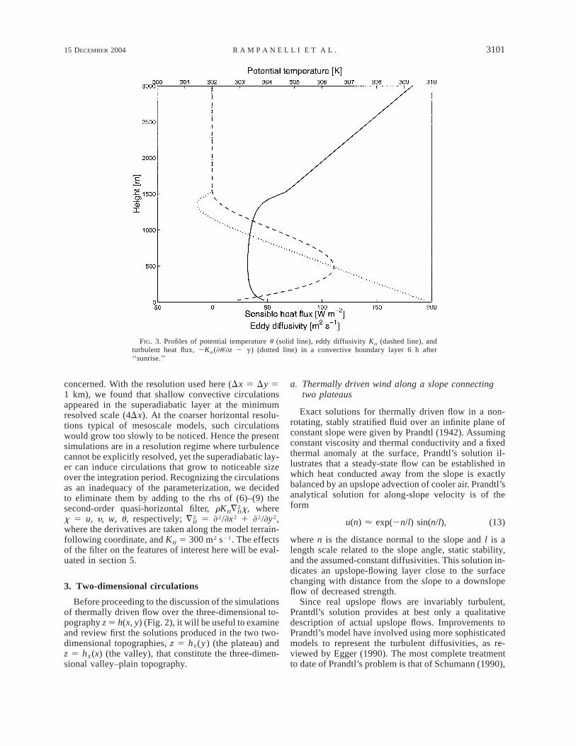
The first thing that happens when a realistically largeheating is applied to the ground surface is that a su-peradiabatic layer forms. Since the resolution used here(Dx 5 Dy 5 1 km and 100 z levels up to H 5 5000m) is far too coarse to simulate directly the ensuingturbulent motions, recourse must be made to a param-eterization. Hence the philosophy of this model and oth-ers of its type (e.g., McNider and Pielke 1981) is thatthe domain and resolution are chosen to resolve the flowfeatures that are on the scale of the topography, but theeffects of vertical turbulent heat transfer must be some-how represented. Therefore, a fundamental buildingblock for understanding the valley wind is a knowledgeof the behavior of the convective boundary layer.

In keeping with the philosophy of the present workof using simple but realistic models, we use the schemedeveloped by Troen and Mahrt (1986, hereafter referredto as TM) in the WRF model to represent the effects ofconvective heat transfer in the vertical direction. Thereis a wealth of knowledge on the simple case of thegrowth of the mixed layer under light wind conditionsover flat horizontally homogeneous terrain (see, e.g.,Stull 1988), and the simple TM model provides an ex-cellent first approximation to the behavior of the con-vective boundary layer. Figure 3 shows the solution forpotential temperature u (5Tp) from the WRF modelsimulating the case of an atmosphere over flat, uniformterrain using the TM boundary model and heating spec-ified as in (12). As explained in TM, the basic featuresof the convective boundary layer are captured by theparameterization, such as a vertical heat flux profile thatis a nearly linear function of height and, consequently,a vertical profile of u that is nearly constant (‘‘wellmixed’’) in a boundary layer capped by an inversion atthe top.

Although the profiles shown in Fig. 3 are realisticrepresentations of the convective boundary layer, theshallow superadiabatic layer produced near the groundis an unstable situation as far as a mesoscale model is


FIG. 3. Profiles of potential temperature u (solid line), eddy diffusivity Km (dashed line), andturbulent heat flux, 2Km(]u/]z 2 g ) (dotted line) in a convective boundary layer 6 h after‘‘sunrise.’’

concerned. With the resolution used here (Dx 5 Dy 51 km), we found that shallow convective circulationsappeared in the superadiabatic layer at the minimumresolved scale (4Dx). At the coarser horizontal resolu-tions typical of mesoscale models, such circulationswould grow too slowly to be noticed. Hence the presentsimulations are in a resolution regime where turbulencecannot be explicitly resolved, yet the superadiabatic lay-er can induce circulations that grow to noticeable sizeover the integration period. Recognizing the circulationsas an inadequacy of the parameterization, we decidedto eliminate them by adding to the rhs of (6)–(9) thesecond-order quasi-horizontal filter, rKH x, where2¹H

x 5 u, y, w, u, respectively; 5 ]2/]x2 1 ]2/]y2,2¹H

where the derivatives are taken along the model terrain-following coordinate, and KH 5 300 m2 s21. The effectsof the filter on the features of interest here will be eval-uated in section 5.

3. Two-dimensional circulations

Before proceeding to the discussion of the simulationsof thermally driven flow over the three-dimensional to-pography z 5 h(x, y) (Fig. 2), it will be useful to examineand review first the solutions produced in the two two-dimensional topographies, z 5 hY(y) (the plateau) andz 5 hX(x) (the valley), that constitute the three-dimen-sional valley–plain topography.

a. Thermally driven wind along a slope connectingtwo plateaus

Exact solutions for thermally driven flow in a non-rotating, stably stratified fluid over an infinite plane ofconstant slope were given by Prandtl (1942). Assumingconstant viscosity and thermal conductivity and a fixedthermal anomaly at the surface, Prandtl’s solution il-lustrates that a steady-state flow can be established inwhich heat conducted away from the slope is exactlybalanced by an upslope advection of cooler air. Prandtl’sanalytical solution for along-slope velocity is of theform

u(n) ø exp(2n/l) sin(n/l), (13)

where n is the distance normal to the slope and l is alength scale related to the slope angle, static stability,and the assumed-constant diffusivities. This solution in-dicates an upslope-flowing layer close to the surfacechanging with distance from the slope to a downslopeflow of decreased strength.

Since real upslope flows are invariably turbulent,Prantdl’s solution provides at best only a qualitativedescription of actual upslope flows. Improvements toPrandtl’s model have involved using more sophisticatedmodels to represent the turbulent diffusivities, as re-viewed by Egger (1990). The most complete treatmentto date of Prandtl’s problem is that of Schumann (1990),


FIG. 4. Solution at t 5 6 h in the case of a two-dimensional plateau for the (a) along-slope windcomponent, (b) vertical wind component, (c) eddy diffusivity, and (d) potential temperature.

who used a large eddy simulation (LES) model to sim-ulate turbulent heat transfer over an infinitely long slopeand found that for small slope angles (#108) a well-mixed layer is formed, which causes a strong temper-ature inversion and a strong downslope flow at the outeredge of the unstable boundary layer.

A further significant complication to Prandtl’s modelis that real slopes are of finite horizontal extent. Theinfinitely long and constant slope of Prandtl’s problempermits the simple rotation of coordinates that allowsPrandtl’s analytical solutions and makes feasible Schu-mann’s (1990) LES calculation. Further progress towardunderstanding the factors affecting real slope flows hasdepended on analytical (Egger 1987a,b) and numericalsimulations of flows over finite-extent slopes such asrepresented by (2), but using a parameterization for theturbulent transfers since LES over such large domainsis not viable (e.g., McNider and Pielke 1981; Segal etal. 1987). Such is the approach adopted here.

Figure 4 illustrates the flow produced at t 5 6 h byimposing the heat flux described by (12) along the to-pography represented by (2). The structure of the up-slope flow is similar to the classical infinite-slope so-lutions described above with a maximum upslope ve-locity near the ground and return flow aloft (Fig. 4a).The vertical structure of the slope flow can be charac-terized as a well-mixed layer of upslope flow topped bya return flow stronger than expected from Prandtl’s so-lution, consistent with Schumann’s (1990) LES calcu-lation. However, as can be seen in Fig. 4, the mostimportant departure from the Prandtl model is the pres-ence of the plateaus. Far from the slope region, well-mixed layers grow (Fig. 4d) since there is no balancing

tendency provided by along-slope cold-air advection.Consistent with the latter is the fact that the mixed layeris shallower over the slope (Figs. 4c,d). Further resultson solution sensitivity to the initial stability, slope, andheating intensity can be found in Ye et al. (1987) andKuwagata and Kondo (1989). Incidentally, the local up-draft maximum located near y 5 20 km in Fig. 4b is atransient feature associated with the leading edge of thecool air that has risen up the slope during the previous6 h.

b. Thermally driven flow in a valley with a horizontalfloor

With the valley topography (3) there is now the ad-ditional effect of two slope flows drawing air from acommon central location, producing a compensatingsubsidence in the valley. This effect is illustrated in Fig.5, where the solutions are shown at t 5 6 h, producedas in the previous case with the heat flux (12) but nowapplied along the valley topography (3). Figure 5 showsthat the flow is upslope along the valley sidewalls; thereis compensating subsidence in the core of the valley,with a vertical velocity of 0(20.1 m s21). Notice thatthe subsidence region extends well above the height ofthe sidewalls (Fig. 5b). The thermal structure inside thevalley displays a mostly stable core region, with twolayers near the sidewalls where the slope flow has de-veloped. This behavior is in agreement with previousexperimental and numerical studies (Bader and McKee1983, 1985; Rampanelli and Zardi 2004). Figure 5dshows that in the valley a well-mixed layer can be iden-tified only in its lower part. In fact, comparing the field


FIG. 5. As in Fig. 4 except for a two-dimensional valley.

of Km(x, z) (Fig. 5c) with that of u(x, z) (Fig. 5d) showsthat u has been modified below z ø 2000 m for all x,even though the layer in which Km ± 0 in the valleycenter only extends to z ø 1400 m. This comparisonsuggests that the advective heat transport plays a crucialrole in producing the observed thermal structure, es-pecially in the core region of the valley (Kondo et al.1989; Noppel and Fiedler 2002). This advective heattransport will be further investigated in section 5c. Atthis display time of 6 h two transient updraft features,analogous to that seen in Fig. 4b, have propagated outof the domain and hence are not evident in Fig. 5b.

4. Thermally driven wind in a valley–plain system

In this section we describe the numerical solution withheating (12) applied along the full valley–plain topog-raphy h(x, y) shown in Fig. 2. By design h(x, y) is theproduct of the slope connecting two plateaus hY(y) andthe two-dimensional valley hX(x) for which the two-dimensional solutions were discussed in the previoussection. As a consequence the three-dimensional solu-tions can be mostly understood as a composite of thetwo-dimensional plateau and valley solutions (Figs. 4–5) individually considered. However, as we shall dem-onstrate below, the valley wind is a uniquely three-di-mensional feature of the solution in the valley–plaincase.

Figures 6–8 show the solution at t 5 6 h in cross-valley planes located at three along-valley positions.Starting from the valley end (Fig. 6), one observes thatthe wind field is nearly identical to the two-dimensionalvalley simulation (Fig. 5). Moving closer to the valley

mouth at y 5 20 km, Fig. 7 shows that, while the cross-valley circulation is similar to that at the valley end,there is now an up-valley flow for all x, and for z ap-proximately less than 1 km; there is down-valley flowat higher altitudes. The along-valley wind speed is high-est near the ground and shows a clear negative minimumin the region of the valley mouth (Fig. 8b). The sub-sidence region in the valley core occurs throughout thevalley atmosphere, from the mouth to the end, and thesubsequent downward heat transfer produces a stableboundary layer throughout the entire valley core, as inthe two-dimensional case (Fig. 5). This effect is evidentwhen comparing panels (e) and (f ) of Figs. 6–8, showingthat the upward turbulent heat transfer from the groundis limited to the lower part of the boundary layer andthat in the upper part, where the subsidence effect isstronger, a different mechanism is at work, as discussedin relation to Fig. 5.

Figures 9–10 show the solution at t 5 6 h in along-valley planes located on the side of the domain locatedat x 5 27.5 km and at the valley center (x 5 0), re-spectively. The solution at the side of the domain (Fig.9) is very similar to the two-dimensional solution forthe plateau (Fig. 4) except that, owing to the valleycirculation, there is outflow (inflow) at low (upper) lev-els over the upper plateau (Fig. 9a). The solution alongthe valley center (Fig. 10) is unlike either of the two-dimensional solutions shown in Figs. 4–5. Figures 10band 10d show the up-valley wind reaching 2 m s21 atthe ground at low levels with a slightly stronger returnflow aloft. The subsidence shown in Fig. 10c beginsnear the valley mouth (y 5 0) and is clearly associatedwith divergence in the cross-valley plane (Figs. 6–8).


FIG. 6. Cross-valley sections at y 5 120 km (valley end) at t 5 6 h in the case of the three-dimensionalplain–valley topography of the (a) cross-valley wind component; (b) along-valley wind component; (c) verticalwind component, the region with w $ 10.005 m s21 is indicated with a dotted line; (d) wind vectors; (e)eddy diffusivity; and (f ) potential temperature.

This subsidence affects the thermal structure of theboundary layer, as may be seen by comparing Figs. 9fand 10f: The boundary layer in Fig. 9f is mainly co-incident with the layer in Fig. 9e where Km ± 0; theboundary layer in Fig. 10f also coincides with the layerwhere Km ± 0 over the plain; however, in the valley itis strongly influenced by the subsidence effect. Thissignificant potential temperature anomaly above the val-ley-top level (z 5 1 km) means that any attempt tocalculate the mean temperature of air within the valleyvolume by simple estimates (such as the topographicalamplification factor, discussed in section 1) must cometo terms with the possibility of a significant heat fluxthrough the top of the valley volume.

5. Explanation of the valley wind

a. Acceleration of the wind along the valley

Because the valley floor along the valley center ishorizontal, the only effect that could produce an along-valley wind there from a state of rest is the along-valley

pressure gradient ]p/]y at x 5 0. Assuming hydrostaticbalance in (8), using the last relation of (10), integratingin z, and then differentiating the result in y leads to

H]p ]p g ] 1ø 1 dz9. (14)E)]y ]y c ]y upz5H z

Analysis of the results indicates that the horizontal pres-sure gradient at z 5 H is negligible; therefore neglectingthe first term on the rhs of (14) we can estimate thepressure gradient term in (7) as

H]p 1 ]u2c Q ø gQ dz9. (15)p E 2]y u ]yz

The solid line in Fig. 11 shows the term on the lhs of(15) as a function of y evaluated at x 5 z 5 0; it ispositive and reaches a maximum near the valley mouth.This structure is consistent with that of the up-valleywind seen along z 5 0 in Fig. 10b. The dots in Fig. 11show the term on the rhs of (15); the near overlap ofthe dots with the solid curve in Fig. 11 confirms thatthe flow occurs under hydrostatic balance and shows


FIG. 7. As in Fig. 6 except for y 5 20 km.

the central importance of understanding the verticalstructure of the along-valley potential temperature dis-tribution in explaining the valley wind.

Also included in Fig. 11 are the pressure gradientterm and its hydrostatic evaluation at x 5 0 and z 51200 m. The reversal of the sign of the pressure gradientat this upper level is consistent with the occurrence thereof the down-valley wind. This reversal displays a qual-itative similarity with that found in the above-discussedstudies of Prandtl (1942) and Schumann (1990), evenin the absence of any upsloping valley floor. Howeverthe physical mechanisms producing these apparentlysimilar features are quite different. The mechanism forthe elevated layer of downslope flow in Prandtl’s(1942) laminar solution (and its extension to the tur-bulent case) is straightforward: the viscous (turbulent)stress exerted by the thermally driven upslope flow onthe layer above it induces adiabatic cooling there; cool-ing through diffusion of yet higher layers must even-tually be balanced at steady state by downslope-flowadiabatic warming. In the present case there is zeroground slope along the valley axis and, as shown with(15), all along-valley motions must be driven by thevertical integral of ]u/]y. Figure 10f indicates that, for

z . 1800 m, ]u/]y , 0, which, as shown by (15) andFig. 11, contributes to a down-valley pressure gradientacceleration at upper levels. Through an analysis of theheat budget below, we demonstrate that the temperaturedistribution shown in Fig. 10f, which drives both theup- and down-valley winds, is a unique feature of thethree-dimensional valley–plain circulation.

b. Comparison with observations

Figure 12 shows vertical profiles of u on the valleyaxis (x 5 0) over the plain (y 5 280 km) and withinthe valley (y 5 120 km). As shown in Fig. 12, thereare significant differences between the classical verticalprofile of potential temperature over plain (cf. Fig. 12with Fig. 3) and that within the valley. The depth-av-eraged temperature difference (difference between ini-tial and final) over the plain is roughly 2.08C, while thatwithin the valley is roughly 3.38C. Table 3 of Vergeinerand Dreiseitl (1987) indicates that the barometric meantemperature difference (in summer) is 2.18C in Munich(the plain) while it is 4.08C at Innsbruck (the valley).Since the measured difference is for the entire heatingperiod (9 h) and our simulations were carried out only


FIG. 8. As in Fig. 6 except for y 5 0 km (valley mouth).

for 6 h, the relative weakness of the simulated excess(3.38 2 2.08C) might be explained. Consistent with thisweakness in the simulated temperature excess in thevalley is the fact that the simulated maximum up-valleywind is only 2 m s21, while the observations in Fig. 3of Vergeiner and Dreiseitl (1987) show values closer to6 m s21. We have carried out our simulations for a periodof 9 hours and find that the depth-averaged temperatureexcess does not increase much after the initial 6 h, andthe averaged temperature of the valley atmosphere re-mains roughly 1.48C warmer than over the plain. In factthe two depth-averaged temperatures’ differences reach3.68C over the plain and 5.08C in the valley. Due to thisnearly constant temperature unbalance between valleyand plain, the maximum up-valley wind does not in-crease much after the initial 6 h of simulation, reaching2.1 m s21, but the region where the up-valley wind isblowing becomes wider in the along-valley direction.

The obtained values are still on the low side; however,it should be kept in mind that the Inn Valley has a sloperoughly 1 in 500. We carried out simulations with avalley slope of 1 in 500 and found in a 6-h simulationthat the depth-averaged temperature excess increased to(4.28 2 2.08C) and the maximum up-valley wind in-

creases to 2.6 m s21. Hence we believe that the presentsimulations are at least roughly consistent with the ob-servations.

Finally, contemporaneosly with the present work,analysis of observations in the Riviera Valley (Rotachet al. 2004) is showing that subsidence heating is a majorcontributor to heating in that valley.

c. Heat budget

Although it is qualitatively clear form Fig. 10 thatsubsidence is a strong contributor to the warming of thevalley core, a quantitative evaluation of the effect isdesirable and is given here. The thermodynamic energybudget within the model atmosphere is given by (9),which can be rewritten as

]u ]u ]u ]u ] ]u5 2u 2 y 2 w 1 K 2 gm1 2[ ]]t ]x ]y ]z ]z ]z

21 K ¹ u. (16)H H

The terms on the rhs of (16) can be separately evaluatedin order to assess the differences between the evolutionof the atmosphere over the plain and that within the


FIG. 9. Along-valley sections at x 5 27.5 km (left side of valley) at t 5 6 h in the case of the three-dimensional plain–valley topography of the (a) cross-valley wind component, (b) along-valley wind com-ponent, (c) vertical wind component, (d) wind vectors, (e) eddy diffusivity, and (f ) potential temperature.

valley. Figure 13a shows the vertical profiles of theterms providing the major contributions to (16) at y 5240, 0, and 80 km, along the valley axis x 5 0. Sinceu 5 0 at x 5 0, only four of the five terms on the rhsof (16) can contribute. In addition, Fig. 13a shows thatat all three locations the along-valley temperature ad-vection is small, so only the latter three terms on therhs side need be considered in the following discussion.

Over the plain (y 5 240 km), Fig. 13a shows thatthe divergence of the turbulent heat flux ]/]z[Km(]u/]z2 g)] is the main contributor to the potential temper-ature tendency and that the remaining terms are negli-gible. In the valley (y 5 0, 80 km), Fig. 13a shows thatthe vertical-advection term is dominant in the upper partof the boundary layer and the turbulent transport is themost important term in the lower part of the layer, wherethe effect of heating from the ground is stronger. Thecombined effect of the vertical advection and the ver-tical turbulent flux of heat produces the modification ofthe vertical structure of the boundary layer shown inFig. 12. Hence vertical advection of potentially warmerair downward from the free atmosphere is the most im-

portant contributor to warming in the upper layers with-in and above the valley region.

As discussed at the end of section 5a, at heights abovez ø 1800 m, Fig. 10f indicates that the valley atmo-sphere is relatively cool with respect to that of the plain.Here we take a closer look at both this relative coolingand the reasons for it. Figure 12 provides a comparisonbetween vertical profiles of potential temperature takenover the plain (y 5 280 km) with those well within thevalley (y 5 120 km) at the mature stage of the valleywind (t 5 6 h); Fig. 12 shows that the valley becomescooler than that over the plane above z ø 1800 m. Thisfigure, together with the u distribution shown in Fig.10f, implies that ]u/]y changes from positive to negativenear z ø 1800 m. The heat budget at the same location(Fig. 13a) shows that the cool air aloft is due to risingmotion there. The rising motion at upper levels in thevalley core is induced by the meeting of the return flowsof the opposing slope flows occurring on the valley walls(Figs. 6–8). The height of the latter is to a first ap-proximation the height of the boundary layer over theplateaus surrounding the valley. With the establishment


FIG. 10. As in Fig. 9 except for x 5 0 km (valley center).

FIG. 11. Along-valley pressure gradient acceleration at the valleycenter, 2cpQ]p/]y (solid lines) from the model output along withgQ (1/u2)]u/]y dz9, which is the pressure gradient accelerationH#z

assuming hydrostatic balance (dots). Upper and lower curves referto evaluation at z 5 0 and 1200 m, respectively.

FIG. 12. (a) Vertical profiles of potential temperature along thevalley axis (x 5 0 m) over the plain (y 5 280 km, solid line) andin the valley region (y 5 120 km; bullet line) at t 5 6 h. The darksolid line shows the initial profile.


FIG. 13. Vertical profiles of the terms in the energy budget (16) (a) at y 5 260, 0, 80 km in themiddle of the valley: turbulent heating, ]/]z[Km(]u/]z 2 g )] (solid line); vertical advection w]u/]z(dotted line); along-valley advection y]u/]y (diamond line); and the numerical filter KH u (bullet2¹H

line) and (b) at y 5 80 km and x 5 3, 6 km. Labeling convention is the same as in (a), exceptadvection represents vertical and along-slope contributions.


of a region of ]u/]y , 0 along the valley axis, we cansee through (15) and Fig. 11 the reasons for a down-valley wind at upper levels along the valley center.

It is interesting to note here that the occurrence ofsuch an upper counterflow and the governing physicalmechanisms have been the subject of a long and con-troversial debate between scientists at the early stagesof valley wind studies. Wagner (1938, his section 5),commenting on the upper-level down-valley wind, iden-tified as a contributing factor (among others) the exis-tence of potentially cooler air above the relatively warmvalley boundary layer; he further speculated that thepotential cool air is produced there by upward verticalmotion resulting from the convergence of the two op-posing return flows associated with the upslope flowson the valley walls. Hence Wagner’s (1938) explanationis in substantial agreement with the present findings.

Figure 13a shows that the effect of the numerical filteris to cool the valley center; this cooling is consistentwith the fact that the effects described above tend toproduce maximum u in the valley center [panel (f ) ofFigs. 6–10]. Hence the effect of the filter is simply toreduce the horizontal gradient of u and, through (16),reduce the magnitude of the simulated valley wind, butotherwise does not effect the fundamental interpretationof the valley wind given here.

The heat budgets within the valley at y 5 80 km onthe slope and at the valley top are shown in Fig. 13b.The heat budget at x 5 3 km (midslope) indicates anear balance between turbulent heating and along-slopeadvection, reminiscent of the Prandtl model; the heatbudget at x 5 6 km (valley top) also indicates a roughbalance between turbulent heating and along-slope ad-vection. In all cases there is a net positive tendencysince the heating is still in progress at 6 h.

6. Conclusions

In the present work we have reconsidered the basicphysical mechanisms governing the daytime evolutionof up-valley winds in mountain valleys. Using a seriesof numerical simulations of thermally driven flow overidealized three-dimensional topography, we have beenable to evaluate the mechanisms of excess valley heat-ing, which, through the hydrostatic law, implies an up-valley acceleration of air from an adjacent plain. Inparticular, our analysis of the numerical solutions showsthat the compensating subsidence in the valley centeris the most important contributor to this excess heating.This mechanism in which subsidence in the valley pro-duces the valley–plain temperature contrast improveson the current textbook description based on bulk ther-modynamics arguments.

The understanding of valley winds developed herehas several important implications. For example, thestability of the atmosphere above the valley is expectedto be an important factor since it will effect the subsi-dence heating within the valley. Another implication is

that the up-valley wind can occur even in a valley withvertical sidewalls (valley volume 5 plain volume), sinceit is to be expected that there would still be compen-sating subsidence at the valley center in such a valley.The results here suggest that the subsidence effect willproduce noticeable differences in the observed verticalstructure of the convective boundary layer within andoutside of a valley (Rampanelli and Zardi 2004; Rotachet al. 2004).

Since the desire here was to deepen our understandingof the dynamics of the up-valley wind, we have inten-tionally limited this study to a topography based on pa-rameters that approximately describe typical mountain–valley situations. An important following step would beto carry out a systematic and more comprehensive seriesof numerical solutions varying the topographical param-eters over the range of observed values.

Perhaps the most fundamental limitation of the pres-ent study is its reliance on a parameterization to simulatethe turbulent convective heat transfer from the groundinto the atmosphere. A simulation of the thermally driv-en flow using the technique of large eddy simulation asin Schumann (1990) would require a grid with muchfiner horizontal resolution (;50 m) and, accordingly, amuch smaller time step (1.2 s); such a calculation wouldbe about 8000 times more costly than the three-dimen-sional computation reported on here. While costly, suchcalculations are presently possible and should be pur-sued in order to cover the gap between the smallestmesoscale phenomena, which can be explicitly resolvedby numerical weather prediction models, and smaller-scale phenomena such as turbulence, which can be ex-plicitly treated only by large eddy simulation models.

Finally we state again that, in order to isolate themechanisms of up-valley winds in their purest form, anumber of practically important effects have been ne-glected, such as the occurrence of an initial stably strat-ified layer capped by a ground-based inversion (cf.Whiteman 1982; Whiteman and McKee 1982; Bader etal. 1987), surface stress, an upward-sloping valley floor,the Coriolis effect, nonuniform insolation depending onthe orientation of the valley axis with respect to sunangle (Whiteman et al. 1989a,b) as well as on shadingby surrounding mountains’ shape (Colette et al. 2003).The relative importance of those effects to the one stud-ied here needs to be determined in future work.

Acknowledgments. This work has been partly sup-ported by the Provincia Autonoma di Trento under theproject PAT-UNITN 2001 and by granting a leave ofabsence to G. Rampanelli for completing his Ph.D. pro-gram. We acknowledge the Mesoscale and MicroscaleMeteorology Division for its support of a visit by D.Zardi to NCAR, and the Department of Civil and En-vironmental Engineering for its support of a visit by R.Rotunno to the University of Trento, which made thiswork possible.


REFERENCES

Bader, D. C., and T. B. McKee, 1983: Dynamical model simulationsof the morning boundary layer development in deep mountainvalleys. J. Climate Appl. Meteor., 22, 341–351.

——, and ——, 1985: Effects of shear, stability and valley charac-teristics on the destruction of temperature inversions. J. ClimateAppl. Meteor., 24, 805–815.

——, ——, and G. J. Tripoli, 1987: Mesoscale boundary layer evo-lution over complex terrain. Part I: Numerical simulation of thediurnal cycle. J. Atmos. Sci., 44, 2823–2837.

Colette, A., F. Katopodes, and R. L. Street, 2003: A numerical studyof inversion-layer breakup and the effects of topographic shadingin idealized valleys. J. Appl. Meteor., 42, 1255–1272.

Defant, F., 1949: Zur theorie der Hangwinde, nebst Bemerkungen zurTheorie der Berg- und Talwinde. Arch. Meteor. Geophys. Biok-lim., A1, 421–450. [English translation: Whiteman, C. D., andE. Dreiseitl, 1984: Alpine Meteorology: Translations of ClassicContributions by A. Wagner, E. Ekhart and F. Defant. PNL-5141/ASCOT-84-3, Pacific Northwest Laboratory, 95–121.]

——, 1951: Local winds. Compendium of Meteorology, T. M. Ma-lone, Ed., Amer. Meteor. Soc., 655–672.

Egger, J., 1987a: Simple models of the valley–plain circulation. PartI: Minimum resolution model. Meteor. Atmos. Phys., 36, 231–242.

——, 1987b: Simple models of the valley–plain circulation. Part II:Flow resolving model. Meteor. Atmos. Phys., 36, 243–254.

——, 1990: Thermally forced flows theory. Atmospheric Processesover Complex Terrain, Meteor. Monogr., No. 45, Amer. Meteor.Soc., 43–57.

Kondo, J., T. Kuwagata, and S. Haginoya, 1989: Heat budget analysisof nocturnal cooling and daytime heating in a basin. J. Atmos.Sci., 46, 2917–2933.

Kuwagata, T., and J. Kondo, 1989: Observation and modeling ofthermally induced up-slope flow. Bound.-Layer Meteor., 49,265–293.

Li, J. G., and B. W. Atkinson, 1999: Transition regimes in valleyairflows. Bound.-Layer Meteor., 91, 385–411.

McNider, R. T., and R. A. Pielke, 1981: Diurnal boundary layerdevelopment over sloping terrain. J. Atmos. Sci., 38, 2198–2212.

Michalakes, J., S. Chen, J. Dudhia, L. Hart, J. Klemp, J. Middlecoff,and W. Skamarock, 2000: Development of a next-generationregional weather research and forecast model. Proc. NinthECMWF Workshop on the Use of Parallel Processors in Me-teorology, ANL/MCS-P868-0101, Reading, United Kingdom,Argonne National Laboratory, 105–107.

Neininger, B., 1982: Mesoklimatische Messungen im Oberwallis(Mesoclimatic measurements in the Upper Valais). Ann. Meteor.,19, 105–107.

Nickus, U., and I. Vergeiner, 1984: The thermal structure of the InnValley atmosphere. Arch. Meteor. Geophys. Bioklim., A33, 199–215.

Noppel, H., and F. Fiedler, 2002: Mesoscale heat transport over com-plex terrain by slope winds—A conceptual model and numericalsimulations. Bound.-Layer Meteor., 104, 73–97.

Prandtl, L., 1942: Fuhrer durch die Stromungslehre. BraunschweighVieweg und Sohn, 407 pp. [English translation: Prandtl, L., 1952:Essentials of Fluid Dynamics. Hafner, 452 pp.]

Rampanelli, G., and D. Zardi, 2004: A method to determine the cap-

ping inversion of the convective boundary layer. J. Appl. Me-teor., 43, 925–933.

Rotach, M. W., M. Andretta, P. Calanca, A. P. Weigel, and R. Vogt,2004: On the turbulence structure over highly terrain: Key find-ings from the MAP-Riviera Project. Extended Abstracts, 11thConf. on Mountain Meteorology, Mt. Washington Valley, NH,Amer. Meteor. Soc., CD-ROM, 6.1.

Schumann, U., 1990: Large-eddy simulation of the up-slope boundarylayer. Quart. J. Roy. Meteor. Soc., 116, 637–670.

Segal, M., Y. Ookuchi, and R. A. Pielke, 1987: On the effect of steepslope orientation on the intensity of daytime upslope flow. J.Atmos. Sci., 44, 3587–3592.

Steinacker, R., 1984: Area–height distribution of a valley and itsrelation to the valley wind. Beitr. Phys. Atmos., 57, 64–71.

Stull, R. B., 1988: An Introduction to Boundary Layer Meteorology.Kluwer Academic, 670 pp.

Troen, I., and L. Mahrt, 1986: A simple model of the atmosphericboundary layer: Sensitivity to surface evaporation. Bound.-LayerMeteor., 37, 129–148.

Vergeiner, I., 1982: Eine energetische theorie der hangwinde (Anenergetic theory of slope winds). Proc. Int. Tagung Alpine Me-teorologie, Tagungsbericht, Berchtesgaden, Germany, 102–105.

——, and E. Dreiseitl, 1987: Valley winds and slope winds—Ob-servations and elementary thoughts. Meteor. Atmos. Phys., 36,264–286.

Wagner, A., 1932: Der taegliche Luftdruck- und Temperaturgang inder freien Atmosphaere und in Gebirgstaelern (The daytime airpressure and temperature variation in the free atmosphere andin mountain valleys). Gerl. Beitr. Geophys., 37, 315–344.

——, 1938: Theorie und Beobachtung der periodischen Gebirgswinde(Theory and observation of periodic mountain winds). Gerl.Beitr. Geophys., 52, 408–449. [English translation: Whiteman,C. D., and E. Dreiseitl, 1984: Alpine Meteorology: Translationsof Classic Contributions by A. Wagner, E. Ekhart and F. Defant,PNL-5141/ASCOT-84-3, Pacific Northwest Laboratory, 11–43.]

Whiteman, C. D., 1982: Breakup of temperature inversion in Colo-rado mountain valleys. Part I: Observations. J. Appl. Meteor.,21, 270–289.

——, 1990: Observations of thermally developed wind systems inmountainous terrain. Atmospheric Processes over Complex Ter-rain, Meteor. Monogr., No. 45, Amer. Meteor. Soc., 5–42.

——, and T. B. McKee, 1982: Breakup of temperature inversion inColorado mountain valleys. Part II: Thermodynamic model. J.Appl. Meteor., 21, 290–302.

——, K. J. Allwine, L. J. Fritschen, M. M. Orgill, and J. R. Simpson,1989a: Deep valley radiation and surface energy budget micro-climates. Part I: Radiation. J. Appl. Meteor., 28, 414–426.

——, ——, ——, ——, and ——, 1989b: Deep valley radiation andsurface energy budget microclimates. Part II: Energy budget. J.Appl. Meteor., 28, 427–437.

Wicker, L. J., and W. C. Skamarock, 2002: Time-splitting methodsfor elastic models using forward time schemes. Mon. Wea. Rev.,130, 2088–2097.

Ye, Z. J., M. Segal, and R. A. Pielke, 1987: Effects of atmosphericthermal stability and slope steepness on the development of day-time thermally induced upslope flow. J. Atmos. Sci., 44, 3341–3354.

Mechanisms of Up-Valley Winds - Ohio Wesleyan...

Documents

Transcript of Mechanisms of Up-Valley Winds - Ohio Wesleyan...