Mechanics of Materials 56 (2013) 23–37

Contents lists available at SciVerse ScienceDirect

Mechanics of Materials

journal homepage: www.elsevier .com/locate /mechmat

Derivation of strain gradient length via homogenizationof heterogeneous elastic materials

Antonios Triantafyllou a,b, Antonios E. Giannakopoulos b,⇑a Laboratory of Reinforced Concrete Technology and Structures, Department of Civil Engineering, University of Thessaly, Volos 38334, Greeceb Laboratory for Strength of Materials and Micromechanics, Department of Civil Engineering, University of Thessaly, Volos 38334, Greece

a r t i c l e i n f o

Article history:Received 31 October 2011Received in revised form 6 June 2012Available online 27 September 2012

Keywords:Strain gradient elasticityHomogenizationMechanical properties

0167-6636/$ - see front matter � 2012 Elsevier Ltdhttp://dx.doi.org/10.1016/j.mechmat.2012.09.007

⇑ Corresponding author. Tel.: +30 24210 74179; faE-mail address: agiannak@uth.gr (A.E. Giannakop

a b s t r a c t

We present explicit upper bound estimates of the microstructural length used in simplegradient elasticity. Our model is a two dimensional composite made of circular hard inclu-sions randomly dispersed in a soft matrix. Both inclusions and matrix are described byisotropic linear elastic constitutive laws. The composite, however, is described by an isotro-pic gradient elastic law. The elastic modulus and the Poisson’s ratio are given by the exactclassic analysis of Christensen. The in-plane microstructural length is estimated by energyoptimization, based on solutions of the gradient elastic hollow cylinder. It was shown thatthe microstructural length decreases with the composition of the particles, taking high val-ues at low particle composition. Naturally, the microstructural length is proportional to theparticle diameter and increases with the stiffness of the particles. It was shown that therecan be no microstructural prediction for particles that are softer than the matrix. This inter-esting result seems to be complementary to the result of Bigoni and Drugan who foundthat, for the couple-stress composite model, there can be no prediction for the microstruc-tural length when the particles are stiffer than the matrix.

� 2012 Elsevier Ltd. All rights reserved.

1. Introduction

The novelty of gradient elasticity theories is theinclusion of an intrinsic length parameter or internallength in the constitutive equations that describe themechanical behavior of the material. The inclusion of thisnew parameter allows these theories to explain the size ef-fect that has been shown experimentally to exist in heter-ogeneous materials. The two simplest and well studiedgradient elasticity theories are the couple stress elasticity(or constraint Cosserat theory) (Mindlin and Tiersten,1962; Koiter, 1964) and the dipolar elasticity theory (orgrade-two theory) (Toupin, 1962; Mindlin, 1964). Themain difference between the two is that in the strain-en-ergy density function that they assume: the first associates

. All rights reserved.

x: +30 24210 74169.oulos).

the internal length with the gradient of the rotations,whereas the second with the gradient of the strains.However, in both theories the internal length is associatedwith the microstresses that are developed due to themicrostructure of the material. In the present work, weemploy the simplest possible dipolar model of just oneadditional length parameter. This choice is based on thefact that one length parameter is enough for predicting sizeeffect and furthermore models with more internal lengthsare both unpractical and difficult to verify experimentally.

A typical composite material consists of a matrix andinclusions. The macroscopic material properties of thecomposite depend on the individual properties of thesetwo phases. The aim of homogenization is to replace thecomposite material with an equivalent material of uniformmacroscopic properties. Micro-mechanical models havebeen developed for both cases of particulate and fiberreinforcement. Among the many homogenization methodsthat have been proposed are the Mori–Tanaka method

24 A. Triantafyllou, A.E. Giannakopoulos / Mechanics of Materials 56 (2013) 23–37

(Mori and Tanaka, 1973), the Self Consistent method(Budiansky, 1965; Hill, 1965), the Generalized Self Consis-tent method (Christensen and Lo, 1979) and the Differen-tial method (McLaughlin, 1977; Norris, 1985). All thesemethods aim at deriving the material properties of elastic-ity which in the case of isotropy are the modulus of elastic-ity and the Poisson ratio. However, when gradient theoriesare considered, an additional material parameter, theinternal length, must be added. Nevertheless, the samestrategy of homogenization can be used, only this time,to yield an estimate for this new parameter.

In the present paper, the elastic energy of the heteroge-neous Cauchy-elastic material will be compared with thatof the homogeneous strain gradient elastic material andthe characteristic length will be estimated as function ofthe inclusion radius, volume fraction and elastic constants.The analysis will be limited to the two-dimensional (2D)case of circular inclusions.

The paper is structured as follows: In Section 2 we pres-ent the classic results for the in-plane effective elasticmoduli (the shear modulus l and the Poisson’s ratio m).In Section 3 we present the elastic energies for the variouscomposite cylinder cases. In Section 4 we present thegradient elasticity solutions for the corresponding compos-ite problem. In Section 5 we give the methodology for theestimation of the internal length and some important re-marks concerning the model are given in Section 6. Finallyin Section 7, we apply our model to an example of steelfiber reinforced concrete mixture and we compare ourestimate with the only other model in the literature thatpredicts the strain gradient internal length parameter.

2. Effective material properties of transversely isotropiccomposites

The following relationships for the effective materialproperties are derived with the generalized self consistentmethod for the specific case cylindrical inclusions, as pre-dicted in Christensen (1990). It is noted that the subscriptm stands for the heterogeneous matrix material and thesubscript i stands for the inclusion. The symbols withoutsubscript are the effective material properties of the homo-geneous material. The overall elastic behavior is that of atransversely isotropic homogeneous material, requiringfive material constants: two of them (l,m) describe theisotropy of the plane (x2, x3) which is of interest in thispaper.

The in-plane shear modulus l, is given by:

Allm

� �2

þ 2Bllm

� �þ C ¼ 0 ð2:1Þ

with

A ¼ 3cð1� cÞ2 li

lm� 1

� �li

lmþ ni

� �

þ li

lmnm þ nmni �

li

lmnm � ni

� �c3

� �

� cnmli

lm� 1

� �� li

lmnm þ 1

� �� �

B ¼ �3cð1� cÞ2 li

lm� 1

� �li

lmþ ni

� �

þ 12

nmli

lmþ li

lm� 1

� �c þ 1

� �

� ðnm � 1Þ li

lmþ ni

� �� 2

li

lmnm � ni

� �c3

� �

þ c2ðnm þ 1Þ li

lm� 1

� �li

lmþ niþ

li

lmnm � ni

� �c3

� �ð2:2Þ

C ¼ 3cð1� cÞ2 li

lm� 1

� �li

lmþ ni

� �

þ nmli

lmþ li

lm� 1

� �c þ 1

� �

� li

lmþ ni þ

li

lmnm � ni

� �c3

� �

nm ¼ 4� 3mm

ni ¼ 4� 3mið2:3Þ

where c is the volume fraction of the inclusions and m de-notes the Poisson ratio.

The in-plain bulk modulus K is:

K ¼ Km þlm

3þ c

1Ki�Kmþð1=3Þðli�lmÞ

þ 1�cKmþð4=3Þlm

ð2:4Þ

The axial modulus E1 (in the x1 direction, normal to the(x2,x3) plane) is:

E1 ¼ cEi þ ð1� cÞEm þ4cð1� cÞðmi � mmÞ2lm

ð1� cÞ lmKiþli=3

� �þ c lm

Kmþlm=3

� �þ 1

ð2:5Þ

The axial Poisson ratio m1 is:

m1 ¼ cmi þ ð1� cÞmm þcð1� cÞðmi � mmÞ lm

Kmþlm=3�lm

Kiþli=3

h ið1� cÞ lm

Kiþli=3

� �þ c lm

Kmþlm=3

� �þ 1

ð2:6Þ

The in-plain Poisson ratio, m, is given by Hashin and Rosen(1964):

m ¼ K � wlK þ wl

ð2:7Þ

where

w ¼ 1þ 4Km21

E1ð2:8Þ

The above solution can be simplified for the two extremecases of rigid inclusions and porous materials. The limitingcase of a porous material can be derived directly fromthe general case represented by (2.2)–(2.8), if we setli = mi = 0.

For the case of fibers much stiffer than the matrix, onlythe coefficients of the li terms in A, B, C of (2.2) need be re-tained with the other being vanishing small. Hence, the A,B, C coefficients, when inclusions are much stiffer than thematrix, take the form:

1.0

1.5

2.0

2.5

3.0

3.5

4.0

4.5

5.0

0% 10% 20% 30% 40% 50% 60% 70% 80% 90% 100%

Composition, c

15/10/5/5.2/2/5.1/

======

mi

mi

mi

mi

mi

mi

μμμμμμμμμμμμ

Shea

r mod

uli r

atio

, μ/μ

m

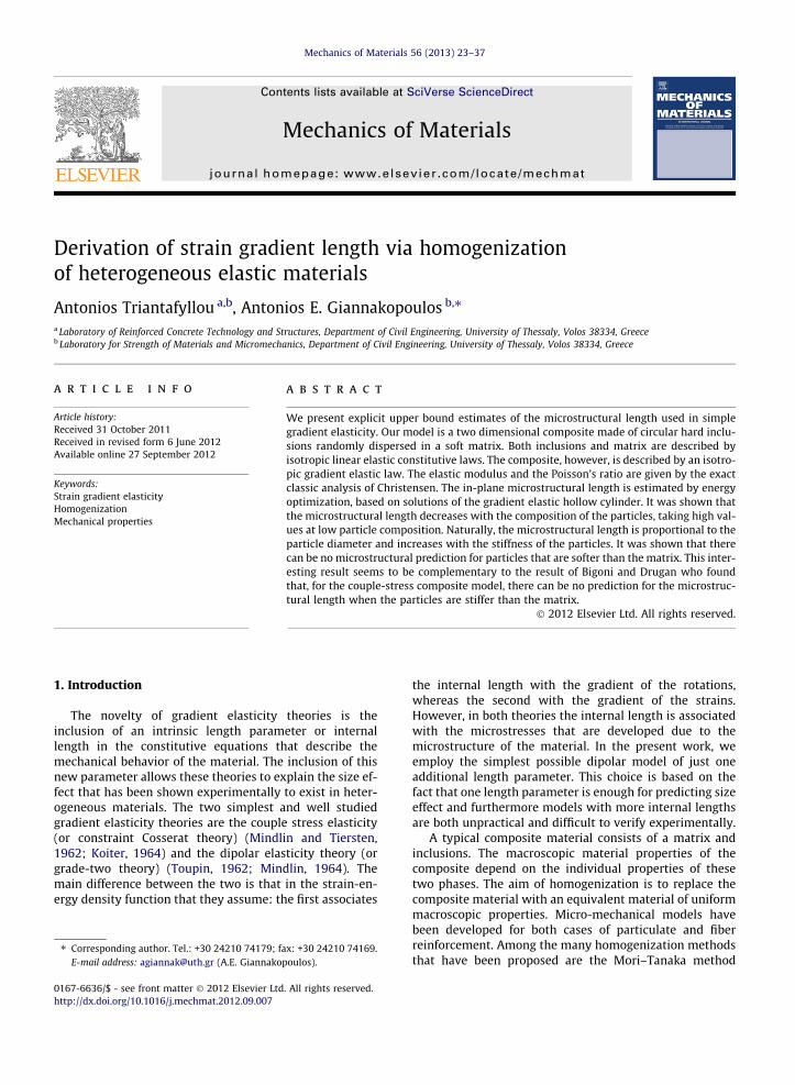
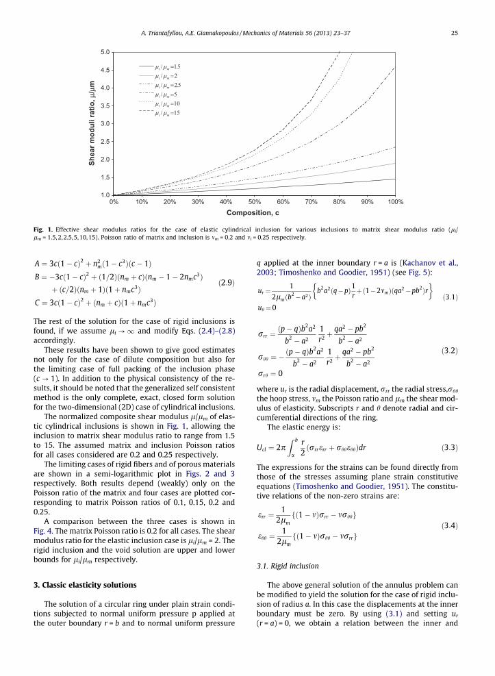
Fig. 1. Effective shear modulus ratios for the case of elastic cylindrical inclusion for various inclusions to matrix shear modulus ratio (li/lm = 1.5,2,2.5,5,10,15). Poisson ratio of matrix and inclusion is mm = 0.2 and mi = 0.25 respectively.

A. Triantafyllou, A.E. Giannakopoulos / Mechanics of Materials 56 (2013) 23–37 25

A ¼ 3cð1� cÞ2 þ n2mð1� c3Þðc � 1Þ

B ¼ �3cð1� cÞ2 þ ð1=2Þðnm þ cÞðnm � 1� 2nmc3Þþ ðc=2Þðnm þ 1Þð1þ nmc3Þ

C ¼ 3cð1� cÞ2 þ ðnm þ cÞð1þ nmc3Þ

ð2:9Þ

The rest of the solution for the case of rigid inclusions isfound, if we assume li ?1 and modify Eqs. (2.4)–(2.8)accordingly.

These results have been shown to give good estimatesnot only for the case of dilute composition but also forthe limiting case of full packing of the inclusion phase(c ? 1). In addition to the physical consistency of the re-sults, it should be noted that the generalized self consistentmethod is the only complete, exact, closed form solutionfor the two-dimensional (2D) case of cylindrical inclusions.

The normalized composite shear modulus l/lm of elas-tic cylindrical inclusions is shown in Fig. 1, allowing theinclusion to matrix shear modulus ratio to range from 1.5to 15. The assumed matrix and inclusion Poisson ratiosfor all cases considered are 0.2 and 0.25 respectively.

The limiting cases of rigid fibers and of porous materialsare shown in a semi-logarithmic plot in Figs. 2 and 3respectively. Both results depend (weakly) only on thePoisson ratio of the matrix and four cases are plotted cor-responding to matrix Poisson ratios of 0.1, 0.15, 0.2 and0.25.

A comparison between the three cases is shown inFig. 4. The matrix Poisson ratio is 0.2 for all cases. The shearmodulus ratio for the elastic inclusion case is li/lm = 2. Therigid inclusion and the void solution are upper and lowerbounds for li/lm respectively.

3. Classic elasticity solutions

The solution of a circular ring under plain strain condi-tions subjected to normal uniform pressure p applied atthe outer boundary r = b and to normal uniform pressure

q applied at the inner boundary r = a is (Kachanov et al.,2003; Timoshenko and Goodier, 1951) (see Fig. 5):

ur ¼1

2lmðb2�a2Þ

b2a2ðq�pÞ1rþð1�2mmÞðqa2�pb2Þr

�

uh ¼0ð3:1Þ

rrr ¼ðp� qÞb2a2

b2 � a2

1r2 þ

qa2 � pb2

b2 � a2

rhh ¼ �ðp� qÞb2a2

b2 � a2

1r2 þ

qa2 � pb2

b2 � a2

rrh ¼ 0

ð3:2Þ

where ur is the radial displacement, rrr the radial stress,rhh

the hoop stress, mm the Poisson ratio and lm the shear mod-ulus of elasticity. Subscripts r and h denote radial and cir-cumferential directions of the ring.

The elastic energy is:

Ucl ¼ 2pZ b

a

r2ðrrrerr þ rhhehhÞdr ð3:3Þ

The expressions for the strains can be found directly fromthose of the stresses assuming plane strain constitutiveequations (Timoshenko and Goodier, 1951). The constitu-tive relations of the non-zero strains are:

err ¼1

2lmfð1� mÞrrr � mrhhg

ehh ¼1

2lmfð1� mÞrhh � mrrrg

ð3:4Þ

3.1. Rigid inclusion

The above general solution of the annulus problem canbe modified to yield the solution for the case of rigid inclu-sion of radius a. In this case the displacements at the innerboundary must be zero. By using (3.1) and setting ur

(r = a) = 0, we obtain a relation between the inner and

1

10

100

0% 10% 20% 30% 40% 50% 60% 70% 80% 90% 100%Composition, c

25.0

20.0

15.0

10.0

====

m

m

m

m

νννν

Shea

r mod

uli r

atio

, μ/μ

m

Fig. 2. Effective shear modulus ratio for the case of cylindrical inclusions much stiffer than the matrix for various matrix Poisson ratio values(mm = 0.1,0.15,0.2,0.25).

0.0

0.1

0.2

0.3

0.4

0.5

0.6

0.7

0.8

0.9

1.0

0% 10% 20% 30% 40% 50% 60% 70% 80% 90% 100%

Porosity, c

0.100.150.200.25=

===

m

m

m

m

νννν

Shea

r mod

uli r

atio

, μ/μ

m

Fig. 3. Effective shear modulus ratio for the case of porous material (lf = mf = 0) for various matrix Poisson ratios (mm = 0.1, 0.15,0.2,0.25).

26 A. Triantafyllou, A.E. Giannakopoulos / Mechanics of Materials 56 (2013) 23–37

outer pressures that satisfies this condition. The innerpressure q must be:

q ¼ 2b2ð1� mmÞpb2 þ a2ð1� 2mmÞ

ð3:5Þ

If we feed this specific value of q back to (3.1) and (3.2), wewill have the solution for the problem of a circular ringcontaining a rigid inclusion.

The elastic energy Ucl1 would then be:

Ucl1 ¼pð1� cÞp2a2 1� mm � 2m2

m

�2lmð1þ mmÞcð1þ c � 2cmmÞ

ð3:6Þ

where c is the composition and is equal to c = a2/b2 for the2D case.

We can rearrange (3.6) to become:

Ucl1 ¼pð1� cÞp2‘2 b

‘

�21� mm � 2m2

m

�2lmð1þ mmÞð1þ c � 2cmmÞ

¼ p� ‘2 � p2 � f1 lm; mm; c;b‘

� �ð3:7Þ

where ‘ is an internal length used to normalize the expres-sion of elastic energy. The addition of this parameter mightappear unnecessary at the moment since it does not affectthe solution but it will become apparent later.

The first derivative of ur at r = b is:

@ur

@r

����r¼b

¼ � ð1þ cÞpð1� 2mmÞ2lmð1þ cð1� 2mmÞÞ

¼ u0rrr ð3:8Þ

3.2. Porous material (voids)

The general solution for the case of pores is directly ob-tained from the general results (3.1) and (3.2), if we setq = 0. The elastic energy is then:

0.0

0.5

1.0

1.5

2.0

2.5

3.0

50%40%30%20%10%0%Volume fraction, c

Shea

r mod

uli r

atio

, μ/μ

m

Rigid inclusion

Elastic inclusion

Void

Fig. 4. Comparison between the cases of porous material and elastic matrix material with rigid or elastic inclusions (li/lm = 2) for mm = 0.2.

Fig. 5. Circular ring subjected to normal uniform external and internalpressures.

A. Triantafyllou, A.E. Giannakopoulos / Mechanics of Materials 56 (2013) 23–37 27

Ucl2 ¼pp2b2ð1þ c � 2mmÞ

2lmð1� cÞ ð3:9Þ

and if we normalize the expression of the elastic energywith the internal length ‘, we obtain:

Ucl2 ¼‘2pp2 b

‘

�2ð1þ c � 2mmÞ2lmð1� cÞ

¼ p� ‘2 � p2 � f2 lm; mm; c;b‘

� �ð3:10Þ

The first derivative of ur at r = b is in this case:

@ur

@r

����r¼b

¼ � pð1� c � 2mmÞ2lmð1� cÞ ¼ u0

rrr ð3:11Þ

3.3. Elastic inclusions

The solution for this case can be obtained by superim-posing the solution of two sub-problems following the wellknown Eshelby methodology (Eshelby, 1957). We firstremove the inclusion and assume an internal pressure qacting at the inner boundary (r = a). By solving this prob-lem we obtain the displacement u(r = a) = u1. We then as-sume a solid circle with the inclusion properties of radiusa under normal pressure q. By solving this problem, we ob-tain the displacement u(r = a) = u2. The two sub-problemsare shown in Fig. 6. The solutions to both these problemscan be easily obtained from the general solution repre-sented by (3.1) and (3.2) by applying the necessary simpli-fications for the second sub-problem.

The radial displacement u1 at r = a of the sub-problem 1,is:

u1 ¼a½qð1þ c � 2cmmÞ � 2pð1� mmÞ�

2lmð1� cÞ ð3:12Þ

The radial displacement u2 at r = a of the sub-problem 2, is:

u2 ¼ �qað1� 2miÞ

2lið3:13Þ

The boundary condition of the generic problem demandsu1 = u2. Using (3.12) and (3.13), we obtain the value of qas a function of the outer pressure p and the material prop-erties of the matrix and inclusion. The pressure q must be:

q ¼ 2plið1� mmÞlmð1� cÞð1� 2miÞ þ lið1þ c � 2cmmÞ

ð3:14Þ

If we feed this value of q back to the solution of the twosub-problems, we obtain the solution of the annulus witha circular inclusion.

The elastic energy of the matrix would then be:

Ucl3 m¼a2ð1�cÞp2p

2clm½ð1�cÞlmð1�2miÞþlið1þc�2cmmÞ�2

� l2mð1�2miÞ2ð1þc�2mmÞþ2ð1�cÞlilm

hð1�2miÞð1�2mmÞþl2

i ð1�2mmÞð1þcð1�2mmÞið3:15Þ

Fig. 6. Superposition of sub-problems 1 and 2 to yield the generic case of an annulus with elastic circular inclusions.

28 A. Triantafyllou, A.E. Giannakopoulos / Mechanics of Materials 56 (2013) 23–37

and, if we normalize the expression of the elastic energywith the internal length ‘, we obtain:

Ucl3 m¼b‘

�2ð1�cÞp2‘2p2lm ð1�cÞlmð1�2miÞþlið1þc�2cmmÞ

�2

� l2mð1�2miÞ2ð1þc�2mmÞþ2ð1�cÞlilm

hð1�2miÞð1�2mmÞþl2

i ð1�2mmÞð1þcð1�2mmÞ�

¼p� ‘2�p2� f3 m lm;mm;li;mi;c;b‘

� �ð3:16Þ

The elastic energy of the inclusions is:

Ucl3 i ¼2a2p2plið1� 2miÞð1� mmÞ2

½ð1� cÞlmð1� 2miÞ þ lið1þ c � 2cmmÞ�2ð3:17Þ

and, if we normalize the expression of the elastic energywith the internal length ‘, we obtain:

Ucl3 i ¼2c b

‘

�2‘2p2plið1� 2miÞð1� mmÞ2

ð1� cÞlmð1� 2miÞ þ lið1þ c � 2cmmÞ �2

¼ p� ‘2 � p2 � f3 i lm; mm;li; mi; c;b‘

� �ð3:18Þ

Therefore, the total elastic energy of an annulus with anelastic circular inclusion is:

Ucl3 ¼ Ucl3 m þ Ucl3 i

¼ p� ‘2 � p2

� f3 m lm; mm;li; mi; c;b‘

� �þ f3 i lm; mm;li; mi; c;

b‘

� �� �ð3:19Þ

and the first derivative of ur at r = b is:

@ur

@r

����r¼b

¼�p ð1þ cÞlið1� 2mmÞ þ lmð1� 2miÞð1� c � 2mm �2lm½ð1� cÞlmð1� 2miÞ þ lið1þ c � 2cmmÞ�

¼ u0rrr

ð3:20Þ

Note that (3.20) gives (3.11) in the case of porous material(li = 0,mi = 0). Also, in the limit of a rigid inclusion(li ?1), (3.20) gives (3.8).

4. Gradient elasticity solution for the annulus problem

Eshel and Rosenfeld (1975) were the first to provide theoutline of the gradient elasticity solution for the annulusproblem. The problem was solved analytically by Aravas(2011) and Gao and Park (2007) for plain strain conditions.The key points of the solution of the annulus problem (seeFig. 2) are presented below.

The material is an in-plane isotropic, compressible,homogeneous, linear elastic material and is described byan elastic strain energy density function W that incorpo-rates strain gradient effects:

Wðe;jÞ ¼ l eijeijþm

1� 2meijeijþ‘2 jijkjijkþ

m1� 2m

jijjjikk

� �h ið4:1Þ

where is ‘ is a material length, e is the infinitesimal straintensor and j the strain gradient 3rd order tensor. Note thatthe deformation in the out-of-plane direction x3 is zero(u3 = 0) and also e33 = 0, j33k = 0.

The Cauchy stress and double stress quantities s and k

are defined as follows:

sij ¼@W@eij¼ 2l eij þ

m1� 2m

eijdij

h iand kijk ¼

@W@jijk

¼ 2l‘2 jijk þm

1� 2mjippdjk

h ið4:2Þ

The following relations also hold true:k ¼ ‘2rsðkijk ¼ ‘2@sij=@xkÞ and j ¼ reðjijk ¼ @eij=@xkÞ

ð4:3ÞThe dynamic boundary conditions required by the princi-pal of virtual work, are the Cauchy (Pr) and the doublestress tractions (Rr) in the radial direction:

PrðrÞ ¼ �c1

2� c6

2r2 � c2‘

rmK1

r‘

� �� ð1� 2mÞK2

r‘

� �h i�

þc3‘

rmI1

r‘

� �� ð1� 2mÞI2

r‘

� �h i� c6

2‘2

r4

)ð4:4Þ

RrðrÞ ¼ �c2‘ ð1� mÞK1r‘

� �þ ð1� 2mÞK2

r‘

� �h i

þ c3‘ ð1� mÞI1r‘

� �� ð1� 2mÞI2

r‘

� �h ið4:5Þ

A. Triantafyllou, A.E. Giannakopoulos / Mechanics of Materials 56 (2013) 23–37 29

where K and I are modified Bessel functions of the first andsecond kind (the subscript shows the order) and c1, c2, c3

and c6 are unknown constants to be determined from thefollowing boundary conditions:

PrðaÞ ¼ �q; RrðaÞ ¼ 0 at r ¼ a

PrðbÞ ¼ �p; RrðbÞ ¼ 0 at r ¼ bð4:6Þ

The radial displacements are:

urðrÞ ¼1

2lð1� 2mÞc1

2r þ c6

2r� ð1� 2mÞ‘

�

� c2K1r‘

� �� c3I1

r‘

� �h ið4:7Þ

and the rest of the solution is:

srrðrÞ ¼ s0rrðrÞ þ

12

c7 �c8

r2

� �þ c2

2K0

r‘

� �þ ð1� 2mÞK1

r‘

� �h i

þ c3

2I0

r‘

� �þ ð1� 2mÞI1

r‘

� �h ið4:8Þ

shhðrÞ ¼ s0hhðrÞ þ

12

c7 þc8

r2

� �þ c2

2K0

r‘

� �� ð1� 2mÞK1

r‘

� �h i

þ c3

2I0

r‘

� �� ð1� 2mÞI1

r‘

� �h ið4:9Þ

and

errðrÞ ¼ e0rrðrÞ þ

12l

ð1� 2mÞ2

c7 �c8

2r2 þ ð1� 2mÞ�

� c2 K0r‘

� �þ ‘

rK1

r‘

� �� �þ c3 I0

r‘

� �� ‘

rI1

r‘

� �� ��

ð4:10Þ

ehhðrÞ ¼ e0hhðrÞ þ

12l

ð1� 2mÞ2

c7 þc8

2r2 � ð1� 2mÞ ‘r

�

� c2K1r‘

� �� c3I1

r‘

� �h ioð4:11Þ

where s0rr ; s0

hh; e0rr and e0

hh represent the classical linear iso-tropic elasticity solution, (i.e. ‘ = 0).

s0rr ¼ Aþ B

r2 ; s0hh ¼ A� B

r2 and u0rr

¼ 12lð1� 2mÞAr � B

r

� �ð4:12Þ

with

A ¼ qa2 � pb2

b2 � a2; B ¼ ðp� qÞ a2b2

b2 � a2ð4:13Þ

and

c1 ¼ c7 þ 2A; c6 ¼ c8 � 2B ð4:14Þ

We are interested in the solution for a ? 0. The constantsc2 and c6 must be zero in order for the displacements tobe finite and zero at r = 0. Therefore, the unknown con-stants reduce to just two, c3 and c7. However, when tryingto calculate the values of these two constants from tractiontype boundary conditions, they both vanish and the gradi-ent solution reduces to the classical elasticity solution. Thisis not surprising because in order for the gradient effects toparticipate in the solution, they must be triggered some-how by the boundary conditions. This is in agreement withthe finding of Bigoni and Drugan (2007) who consideredcorresponding results for Cosserat materials.

In order to overcome this, a kinematic boundary condi-tion is assumed at r = b:

@ur

@r

����r¼b

¼ u0rrr ð4:15Þ

This condition implies that the two dimensional gradientelastic material that represents the composite, assumes ahomogeneous gradient of the radial displacement. We willuse (4.15) together with the traction type condition Pr(b) =�p. In this way we load the gradient material with trac-tions and displacements gradients that are the same withthese of the inhomogeneous classic composite system.

The constants now become:

c8 ¼ c2 ¼ B ¼ 0; A ¼ �p ð4:16Þand

c3 ¼2b½ð1�2mÞpþ2l�u0

rrr �ð1�2mÞ b I0

b‘

�þ I2

b‘

� ��2‘ I2

b‘

�þmI1

b‘

��2mI2

b‘

� � � ð4:17Þ

c7 ¼�4‘ I2

b‘

�þmI1

b‘

��2mI2

b‘

� �ð1�2mÞpþ2l�u0

rrr

�ð1�2mÞ b I0

b‘

�þ I2

b‘

� ��2‘ I2

b‘

�þmI1

b‘

��2mI2

b‘

� � � ð4:18Þ

The elastic energy of the gradient solution Ugr is:

Ugr ¼ pZ b

0r srrerr þ shhehh þ krrrjrrr þ khhhjhhhð Þdr ð4:19Þ

or

Ugr ¼ p‘2Z b=‘

0

r‘

srrerr þ shhehh þ krrrjrrr þ khhhjhhhð Þd r‘

The values of j and k are obtained after substituting (4.8)–(4.11) into (4.3).

After substituting all the quantities and integrating, thegradient elastic energy becomes:

Ugr ¼pð�1þ2mÞp2‘2

4l�1

2c7

p�2

� �2 b‘

� �2(

�12

c3

p

� �2 b‘

� �2

� I20

b‘

� �� I2

1b‘

� �� ��1

2c3

p

� �2 b‘

� �2

� I21

b‘

� �� I0

b‘

� �I2

b‘

� �� �� c3

pc7

p�2

� �b‘

� �2

�HGC 2;14

b‘

� �2" #

þ12

c3

p

� �2

�1þHG12

� ;f1;1g; b

‘

� �2" # !

� c3

p

� �2

�1þHG12

� ;f1;2g; b

‘

� �2" # !

�3c3

p

� �2 b‘ð1þ2mÞHG

12

� ;f2;2g; b

‘

� �2" #

þ c3

p

� �2 b‘ð1�2mÞHG

12

� ; 2;3f g; b

‘

� �2" #

þ2c3

p

� �2 b‘ð1�2mÞHG

12;12

� ; 1;1;

32

� ;

b‘

� �2" #

�13

c3

p

� �2 b‘

� �3

ð1þ2mÞHG32;32

� ; 2;2;

52

� ;

b‘

� �2" #

þ14

c3

p

� �2 b‘

� �3

ð1�2mÞHG32;32

� ; 2;

52;3

� ;

b‘

� �2" #)

ð4:20Þ

30 A. Triantafyllou, A.E. Giannakopoulos / Mechanics of Materials 56 (2013) 23–37

or

Ugr ¼ p� ‘2 � p2 � g l; m; c3; c7; c;b‘

� �

where HG is a generalized hypergeometric function andHGC is a regularized confluent hypergeometric function(Abramowitz and Stegun, 1970). Both functions aredescribed as:

HG½fa1; . . . ; apg; fb1; . . . ; bqg; x� ¼ pFqða; b; xÞ

¼X1k¼0

ða1Þk . . . ðapÞk=ðb1Þk . . . ðbqÞkxk

k!

HGC½a; x� ¼ 0F1ða; xÞ=CðaÞ;

where C(a) is the Euler gamma function.Alternatively, the gradient elastic energy can be found

from the external work. The elastic energy is then equal to:

Ugr ¼ pbfPrðbÞurðbÞ þ RrðbÞu0rðbÞg ð4:21Þ

where primes denote derivatives with respect to r.Substituting the value of u0

rrr from (3.20) into (4.17) and(4.18), we can connect the gradient elasticity solutionswith the classic elasticity solutions for the three cases ofrigid inclusion, porous material and elastic inclusionsdiscussed in Section 3. This approach is similar to that ofBigoni and Drugan (2007) for Cosserat gradient elasticmaterials. We obtain the constants c3 and c7 for each caseseparately:

For the case of rigid inclusions (Fig. 7), the constantsbecome:

c3 1 ¼2b‘p ð1�2mÞ� l

lm

ð1þcÞð1�2mmÞ1þcð1�2mmÞ

h ið1�2mÞ b

‘I0

b‘

�þ I2

b‘

� ��2 I2

b‘

�þmI1

b‘

��2mI2

b‘

� � � ð4:21Þ

c7 1 ¼�4p I2

b‘

�þmI1

b‘

��2mI2

b‘

� �ð1�2mÞ� l

lm

ð1þcÞð1�2mmÞ1þcð1�2mmÞ

h ið1�2mÞ b

‘I0

b‘

�þ I2

b‘

� ��2 I2

b‘

�þmI1

b‘

��2mI2

b‘

� � � ð4:22Þ

For the case of porous materials (Fig. 8), the constantsbecome:

c3 2 ¼2b‘p ð1�2mÞ� l

lm

ð1�c�2mmÞð1�cÞ

h ið1�2mÞ b

‘I0

b‘

�þ I2

b‘

� ��2 I2

b‘

�þmI1

b‘

��2mI2

b‘

� � � ð4:23Þ

c7 2 ¼�4p I2

b‘

�þmI1

b‘

��2mI2

b‘

� �ð1�2mÞ� l

lm

ð1�c�2mmÞð1�cÞ

h ið1�2mÞ b

‘I0

b‘

�þ I2

b‘

� ��2 I2

b‘

�þmI1

b‘

��2mI2

b‘

� � � ð4:24Þ

For the case of elastic inclusions(Fig. 9), the constantsbecome:

c3 3 ¼2

b‘

p ð1� 2mÞ �l ð1þ cÞlið1� 2mmÞ þ lmð1� 2miÞð1� c lm ð1� cÞlmð1� 2miÞ þ lið1þ c � 2cm

"

ð1� 2mÞ b‘

I0b‘

�þ I2

b‘

� �� 2 I2

b‘

�þ mI1

b‘

�� 2mI2

b‘

�

c7 3 ¼�4p I2

b‘

� �þ mI1

b‘

� �� 2mI2

b‘

� �� �ð1� 2mÞ �

l ð1þ cÞlið lm ð1�

"

ð1� 2mÞ b‘

I0b‘

�þ I2

b‘

� �� 2 I2

b‘

�þ m

Note that for all expressions of the constants c3 and c7, theinternal length appears only in the normalized form b/‘. Bysubstituting c3_i and c7_i, with i = 1, 2, 3 to (4.20), we obtainthree expressions for the gradient elastic energy Ugr1, Ugr2

and Ugr3 respectively.

5. Estimation of internal length

The energy of the heterogeneous material calculated inSection 3 and the energy of the gradient homogeneousmaterial calculated in Section 4 were determined for thesame boundary conditions. By equating the two energies,we can derive an estimation of the internal length of thegradient material as a function of the inclusion radiusa,the composition ratio c and the elastic material constantsof the matrix and the inclusion (li/lm,mi,mm). However,before proceeding, we must face the problem of how tosettle the other two material properties of the gradientmaterial which in the general case will not be equal tothe matrix material properties. The problem has three un-knowns, namely, the internal length ‘, the in-plane shearmodulus l and the in-plane Poisson ratio m and we onlyhave one equation to work with, which is:

Ucl ¼ Ugr ð5:1Þ

If the solution is limited to dilute concentration of inclu-sions one can assume that the material properties of thematrix and composite material remain the same. It is notedthat the results of Bigoni and Drugan (2007) were derivedusing this assumption. In this work the two material prop-erties, i.e. the shear modulus and Poisson ratio, wereextracted from a classic composite model suitable to ourconsidered problem. By doing so, the unknowns arereduced to just one, the internal length ‘, which can thenbe estimated. This approach is justified by the fact thatthe gradient material should always reduce to the classicmaterial if the gradient effect is neglected, i.e. ‘ = 0. There-fore the effective material properties predicted by theclassical homogenization schemes hold true for the com-posite gradient material as well. Estimates of the effectivematerial properties of the homogeneous gradient materialthat correspond to our problem are given in Section 2.

The expression of Ugr is highly non-linear and can not besolved explicitly with respect to ‘. It can however be solvednumerically through an iteration process for differentvalues of all the parameters. The solution path is shown

� 2mm�

m�

#��

ð4:25Þ1� 2mmÞ þ lmð1� 2miÞð1� c � 2mm

�cÞlmð1� 2miÞ þ lið1þ c � 2cmmÞ

�#

I1b‘

�� 2mI2

b‘

���ð4:26Þ

Fig. 7. Homogenization procedure of a material containing rigid inclusions: (a) Heterogeneous Cauchy material; (b) Homogeneous gradient material.

Fig. 8. Homogenization procedure of a porous material: (a) Heterogeneous Cauchy material; (b) Homogeneous gradient material.

Fig. 9. Homogenization procedure of a material containing elastic inclusions: (a) Heterogeneous Cauchy material; (b) Homogeneous gradient material.

A. Triantafyllou, A.E. Giannakopoulos / Mechanics of Materials 56 (2013) 23–37 31

Fig. 10. Iteration process to estimate the internal length as a function of the composition, c, and the inclusion radius, a.

Table 1Variation of the normalized gradient internal length for the case of rigid inclusions.

c b/‘ ‘/aa

mm = 0.1 mm = 0. 15 mm = 0.2 mm = 0.25 mm = 0.1 mm = 0.15 mm = 0.2 mm = 0.25

0.1% 4.6 4.5 4.5 4.7 6.802 7.088 7.058 6.7071% 7.2 5.4 4.9 5.0 1.390 1.844 2.028 2.0175% 17.1 9.6 7.0 6.1 0.262 0.468 0.640 0.73210% 27.8 14.7 10.2 7.8 0.114 0.214 0.309 0.40820% 47.9 26.4 16.7 12.0 0.047 0.085 0.134 0.18630% 71.7 42.0 26.7 18.6 0.025 0.043 0.068 0.09840% 106.2 66.1 43.1 29.6 0.015 0.024 0.037 0.05350% 163.0 107.3 72.3 50.0 0.009 0.013 0.020 0.02860% 268.2 186.3 130.2 91.7 0.005 0.007 0.010 0.01470% 495.5 362.2 263.6 191.0 0.002 0.003 0.005 0.00680% 1140.7 875.8 664.8 498.6 0.001 0.001 0.002 0.00290% 4583.1 3685.0 2921.5 2277.0 0.000 0.000 0.000 0.000

a For the 2D case, the composition is: c = a2/b2.

0

1

2

3

4

5

6

7

8

100.0%10.0%1.0%0.1%Composition, c

Gra

dien

t int

erna

l len

gth

to in

clus

ion

radi

us

rat

io, ℓ

/α

25.020.015.010.0

====

m

m

m

m

νννν

Fig. 11. Variation of the gradient internal length to the inclusion radius ratio ‘/a, with respect to the composition c, for the case of rigid cylindricalinclusions.

32 A. Triantafyllou, A.E. Giannakopoulos / Mechanics of Materials 56 (2013) 23–37

schematically in Fig. 10. Throughout the calculations, a5-digit accuracy was maintained. The numerical integra-tion of the curves presented below converges as the inter-polation order is increased.

5.1. Rigid inclusions

Estimation for the internal length for rigid inclusions isderived by equating the two associated energies, Ucl1 = Ugr1

0

1

2

3

4

5

6

7

100.0%10.0%1.0%0.1%

Composition, c

Gra

dien

t int

erna

l len

gth

to in

clus

ion

radi

us

r

atio

, ℓ/ α

∞→=====

mi

mi

mi

mi

mi

mi

μμμμμμμμμμμμ

/

15/

10/

5/

2.5/

2/

Fig. 12. Variation of the gradient internal length divided by the inclusion radius with respect to the composition c for the case of elastic cylindricalinclusions (mm = 0.2,mi = 0.25).

Table 2Variation of the normalized gradient internal length for the case of elastic inclusions.

c b/‘a ‘/ab

li/lm = 2 li/lm = 2.5 li/lm = 5 li/lm = 10 li/lm = 15 li/lm = 2 li/lm = 2.5 li/lm = 5 li/lm = 10 li/lm = 15

0.1% 52.5 44.1 16.6 9.4 7.5 0.602 0.717 1.909 3.350 4.1931% 55.5 36.8 16.4 9.8 8.0 0.180 0.272 0.611 1.018 1.2525% 54.6 38.5 18.6 12.0 10.2 0.082 0.116 0.240 0.372 0.44010% 57.3 41.7 21.8 15.0 13.1 0.055 0.076 0.145 0.210 0.24120% 64.3 49.4 29.4 22.4 20.3 0.035 0.045 0.076 0.100 0.11030% 72.5 58.9 39.6 32.5 30.5 0.025 0.031 0.046 0.056 0.06040% 82.5 70.7 54.0 47.9 46.1 0.019 0.022 0.029 0.033 0.03450% 93.9 85.4 74.9 72.4 72.0 0.015 0.017 0.019 0.020 0.02060% 106.7 103.5 106.0 113.6 117.7 0.012 0.012 0.012 0.011 0.01170% 121.2 125.4 153.1 187.4 205.7 0.010 0.010 0.008 0.006 0.00680% 136.4 152.1 227.2 332.6 398.5 0.008 0.007 0.005 0.003 0.00390% 164.5 185.9 – 674.2 938.2 0.006 0.006 – 0.002 0.001

a The Poisson ratio of the matrix and inclusion is 0.2 and 0.25, respectively.b For the 2D case, the composition is: c = a2/b2.

A. Triantafyllou, A.E. Giannakopoulos / Mechanics of Materials 56 (2013) 23–37 33

(see Fig. 7). The variation of the gradient internal length, ‘,normalized by the radius of the inclusion,a, with the com-position ratio c is shown in Fig. 11 in a semi logarithmicplot for mm values of 0.1, 0.15, 0.2 and 0.25. The resultsare also presented in Table 1. We note that the internallength increases with the matrix Poisson ratio.

5.2. Elastic inclusions

Estimation for the internal length for the case of elasticinclusions is derived by equating the two associated ener-gies, Ucl3 = Ugr3 (see Fig. 9). The variation of the gradientinternal length, ‘, normalized by the radius of the inclu-sion, a, with the composition ratio c is shown in Fig. 12in a semi logarithmic plot for inclusion to matrix shearmodulus ratio, li/lm values of 2, 2.5, 5, 10 and 15(mm = 0.2,mi = 0.25). For comparison purposes, the rigid case

with mm = 0.2 is plotted as well. These results are also pre-sented in Table 2. The rigid inclusion case li/lm ?1 givesthe upper bound of ‘/a and ‘/a increases monotonicallywith li/lm > 1. The internal length ‘/a is a decreasing func-tion of composition c, with ‘/a ? 0 as c ? 1, as expected. Itis noted that in all cases, when c ? 0, ‘/a ?1 withR 1

0 ‘=adc finite. Note also that when the ratios li/lm andmi/mm was assumed to be equal to one, no physically mean-ingful prediction was recovered from the problem as itshould, because this case is essentially the case of a homo-geneous material. The same was found to be true when theinclusion is less stiff than the matrix.

5.3. Porous material

Estimation for the internal length for the case of voidsis derived by equating the two associated energies,

34 A. Triantafyllou, A.E. Giannakopoulos / Mechanics of Materials 56 (2013) 23–37

Ucl2 = Ugr2, (see Fig. 8). The normalized internal length(b/‘) estimate for this case is of the order 10�8, for themajority of c values, and for some values of c the estimateof b/‘ becomes negative. These results can not be accept-able since they lack physical justification. In other words,there can be no realistic prediction for the internal lengthfor the case of porous materials or generally when theinclusions are less stiff than the matrix. When inclusionsare less stiff than the matrix, the micro-structural loadpath changes and strain gradient theories may be no longerapplicable because microstructure with voids introducesgradients mostly in the antisymmetric part (rotations)than in the symmetric part (strains) of the deformationsgradient. This is in agreement with Bigoni and Drugan(2007) who used a couple-stress (constaint Cosserat) mod-el that emphasize on the rotation gradient. They provedthat there can be no prediction for the microstructurallength when particles are stiffer than the matrix. We couldargue that the present results are complementary to thoseof Bigoni and Drugan (2007).

6. Remarks

6.1. Micromechanical explanation of the results

The predictions presented in Section 5 showed that asthe composition is increased, the internal length esti-mates decreases. The internal length is associated withthe microstresses that develop due to the microstructureof the composite. However when composition increasesthe distance between particles, decreases. Instead of hav-ing an inclusion embedded in a continuum, the problemresembles that of a particle with a thin layer around it.It has been shown (Budiansky and Carrier, 1984) thatwhen this happens, the strain gradients reducedrastically.

6.2. Influence of the loading system

The estimates of Section 5 were based on an axi-symmetric type of loading. In order to verify that thesepredictions hold true for other loading cases, we con-sidered a different loading system that removes thissymmetry. The second loading case corresponds to aremote uniaxial tension and the details of the solutionsare presented in Appendix A. We consider the limitingcase of rigid inclusions only and found that the mate-rial length prediction obtained from both loading casesis the same.

7. Application to fiber-reinforced concrete

A hooked end steel fiber reinforced concrete mixture(Papatheocharis, 2007) used currently by Lafarge for retro-fitting structures has the following properties: Em = 40 GPa,mm = 0.2, Ei = 210 GPa, mi = 0.3 and c = 0.8%. The fibers have acircular cross section and the diameter is 5 mm. The shearmodulus ratio of fibers and matrix is: li/lm = 4.85. Thedensity of the matrix is qm = 2350 kg/m3 and the densityof the inclusion/fiber is qi = 7850 kg/m3

In order to obtain the estimate of the internal length,one can use either the assumption of elastic or rigid inclu-sion. The internal length estimate for each case is:

Rigid fiber assumption ?‘/a = 2.3) ‘ = 5.75 mmElastic fiber assumption ?‘/a = 0.6) ‘ = 1.50 mm

It is noted that this specific fiber-reinforced mixturewas designed to be used as an outside jacket to existingreinforced concrete column and this jacket has typically athickness between 3 cm and 5 cm.

7.1. Ben–Amoz estimate of the internal length parameter

The Ben–Amoz model (Ben-Amoz, 1976) for predictingthe internal length parameter is based on a dynamic anal-ysis of the micro and macro-structure. It is noted that inthe absence of the dynamic conditions imposed onproblem, the validity of model becomes questionable. Nev-ertheless, the Ben–Amoz model is the only other model inthe literature that predicts the strain gradient internallength parameter and for this reason it is interesting tocompare the two predictions. The key points of the modelare presented below.

A normalized scale parameter, L/d, is introduced whichcan be seen as a measure of the strength of inhomogeneity.It is noted that this scale parameter is derived by assumingthat the strain energy and kinetic energy are of the sameorder of magnitude but this assumption however is notalways true.

The normalized scale parameter is:

L=d ¼ qtðkþ 2lÞt=qRðkþ 2lÞR �1=2 ð7:1Þ

where, d = 2b for the 2D case.and subscripts t and R denotethe Voigt and Reuss averaging quantities respectively,which are defined as follow:

ðÞt ¼ cmðÞm þ ciðÞi1ðÞR¼ cm

ðÞmþ ci

ðÞið7:2Þ

where c is volume fraction and subscript m and i denotesthe matrix and inclusion/fiber material.

The internal length parameters, ‘1 and ‘2, of Midlin’swork for the long wave-length approximation (Mindlin,1964, pp.69) are then associated with the scale parameterL by the following equations for the shear and dilatationmodes:

‘21 ¼

L2

41� li � lm

ltðci � 4IiÞ

� �

‘22 ¼

L2

41� ðkþ 2lÞi � ðkþ 2lÞm

ðkþ 2lÞtðci � 4IiÞ

� � ð7:3Þ

where for the 2D case Ii ¼ ða=bÞ4 ¼ c2i

By applying the simplifications of the simplified straingradient theory used throughout in this paper (see Mind-lin, 1964, pp. 73, a

_

1 ¼ a_

3 ¼ a_

5 ¼ 0, a_

2 ¼ ðk=2Þ‘2 anda_

4 ¼ l‘2), the Mindlin’s internal length parametersbecome ‘1 = ‘2 = ‘. Hence, the Ben–Amoz model gives twodifferent estimates for the internal length parameter,

A. Triantafyllou, A.E. Giannakopoulos / Mechanics of Materials 56 (2013) 23–37 35

which however for small values of the composition c areapproximately the same. The Ben–Amoz predictions, forthe specific fiber reinforced concrete mixture consideredhere, are:

Shear mode ? ‘/a = 11.28) ‘ = 28.2 mmDilatation mode ? ‘/a = 11.22) ‘ = 28.05 mm

8. Conclusions

The homogenization of a plane-strain heterogeneousCauchy-elastic material was performed and the internallength parameter used in strain gradient theory was esti-mated for the cases of elastic inclusion stiffer than thematrix. Upper bound estimates for the internal length werefound when inclusions much stiffer than the matrix wereconsidered. The internal length was found to be between0.5 and 7 times the inclusion radius for very small valuesof c(c ffi 0.1%) depending on the inclusion to matrix shearmodulus ratio. The internal length decreases rather rapidlyas the composition is increased and is approximately zerofor c > 70%. No prediction was possible for inclusions lessstiff than the matrix and for the extreme case which corre-sponds to porous materials.

Acknowledgments

The current work is part of the ‘‘Hrakleitos II’’ projectof the Greek Ministry of National Education for basicresearch on size effect phenomena. The authors wouldalso like to thank Professor F. Perdikaris for his usefulcomments and Professor N. Aravas for sharing hisfindings.

Appendix A. Remote uniaxial tension case

We consider the problem of a circular inclusion ofradius a inserted into an infinite isotropic body underremote uniaxial tension P as shown in Fig. A.1.

The plain-strain gradient solution for the radial andangular displacements outside the inclusion has been pro-duced by Aravas (Private communication):

Fig. A.1. Inclusion of radius a inserted into an

urðr; hÞ ¼

P4l rð1� 2mþ cosð2hÞÞ

þ Pl

A1ar þ A3

ar þ A5

a‘K1

r‘

� �þ A1

ar þ A2

‘r K2

r‘

�þ A4

ar

�3hþA6

ar K2

r‘

�þ a

2‘ K1r‘

� ��cosð2hÞ

8>><>>:

9>>=>>;

8>>>>><>>>>>:

ðA:1Þ

uhðr; hÞ ¼

� P4l r sinð2hÞ

þ Pl � 1�2m

2ð1�mÞA1ar þ A2

‘r K2

r‘

�þ 1

2 K1r‘

� �nþA4

ar

�3 þ A6ar K2

r‘

�osinð2hÞ

8>>><>>>:

ðA:2Þ

where Ai (i = 1..6) are unknown coefficients.The classical expressions of the displacements outside

the inclusion for the case of rigid inclusions (Kachanovet al., 2003) are:

u0r ðr; hÞ ¼

Pa8l

ðt� 1Þ raþ 2c

ar

h i�

þ 2raþ bðtþ 1Þ a

rþ 2d

ar

� �3� �

cosð2hÞ

ðA:3Þ

u0hðr; hÞ ¼

Pa8l

�2ra� bðtþ 1Þ a

rþ 2d

ar

� �3�

sinð2hÞ ðA:4Þ

where b = �2/t, c = (1 � t)/2, d = 1/t and t = 3 � 4m.Note that both the gradient and classical solutions have

the same dependence on the angle h.We demand that at r = a and r = b (b > a), the gradient

displacements to be equal to the classical prediction:

urða; hÞ ¼ u0r ða; hÞ8h

uhðb; hÞ ¼ u0hðb; hÞ8h

ðA:5Þ

Eq. (A.5) describe a system of six equations that can besolved for the six unknowns Ai. The coefficients thatbecome zero are:

A2 ¼ A5 ¼ A6 ¼ 0 ðA:6Þ

Therefore, the gradient solution reduces to the classicsolution but this however does not mean that the gradienteffect disappears as in the case of axisymmetric loading.In essence we apply the same kinematic admissiblefield to the gradient homogeneous material and classic

infinite body under uniaxial tension P.

0

1

2

3

4

5

6

7

10.0%1.0%0.1%Composition, c

Gra

dien

t int

erna

l len

gth

to in

clus

ion

radi

us

ratio

, ℓ/ α

Loading case 1

Loading Case 2

Fig. A.2. Variation of the gradient internal length to the inclusion radius ratio ‘/a, with respect to the composition c, for the case of rigid cylindricalinclusions, obtained for two different loading cases (mm = 0.2).

36 A. Triantafyllou, A.E. Giannakopoulos / Mechanics of Materials 56 (2013) 23–37

heterogeneous material. Therefore, the boundary condi-tions for the two systems at r = a and r = b are the same.Obviously, this kinematic field is the same only for r P a,but for the case of dilute composites (a < <b), the total elas-tic energy calculated for b P r P a is approximately thesame with the total elastic energy calculated for b P r P 0.

The expression for the total elastic energy for the heter-ogeneous classic material is:

Ucl ¼ 4Z p=2

0

Z b

a

12

r srrerr þ shhehh þ 2srherhð Þdrdh ðA:7Þ

The expression of the total elastic energy for the homoge-neous gradient material is:

Ugr ¼ 4Z p=2

0

Z b

a

12

rsrrerr þ shhehh þ 2srherh

þkrrrkrrr þ krhhkrhh þ 2krrhkrrh

þkhrrkhrr þ khhhkhhh þ 2khrhkhrh

0B@

1CAdrdh

ðA:8Þ

It is reminded that the double stress k and the third orderstrains k are defined by Eq. (4.3) accounting that:

r ¼ er@

@rþ eh

1r@

@h;

rs ¼ @srr@r errr þ @shh

@r ereheh þ @srh@r erðereh þ eherÞ

þ 1r

@srr@h � 2srh �

eherer þ 1r

@shh@h þ 2srh �

eheheh

þ 1r

@srh@h þ srr � shh

�ehðereh þ eherÞ

ðA:9Þ

where e is the base vector.Under the assumption of dilute composition, we can de-

mand equality of the two energies since both systems havethe same boundary conditions and the gradient energypart neglected i.e. a P r P 0 is very small if b > > a, i.e.c < < 1. The other two material properties, i.e. in-planeshear modulus and Poisson ratio for the gradient materialare again extracted from the Cristensen predictions (seeSection 2).

The variation of the gradient internal length, ‘, normal-ized by the radius of the inclusion, a, with the compositionratio c is shown in Fig. A.2 for the case of rigid inclusionsand assuming that the matrix Poisson ratio is mm = 0.2.The solid line corresponds to the loading case 1 (seeFig. 7) and the diamond symbols correspond to loadingcase 2 (see Fig. A.1). The prediction for the second loadingcase was derived under the assumption of dilute concen-tration of inclusions and hence we plot only the predic-tions for c < 10%. As can be seen in Fig. A.2, the matchbetween the two estimates is very good at low values ofc and as c increases the two predictions differ as expectedsince the dilute composition assumption is compromised.Nevertheless, the results clearly show that a different load-ing system did not affect the prediction of the internallength parameter.

References

Abramowitz, M., Stegun, A.I., 1970. Handbook of Mathematical Functions,7th ed. Dover Publications, INC., New York.

Aravas, N., 2011. Plane-stain problems for a class of gradient elasticitymodels-a stress function approach. J. Elast. 45, 100–110.

Aravas N. Private communication.Ben-Amoz, M., 1976. A dynamic theory for composite materials. J Appl.

Math. Ph. (ZAMP) 27, 83–99.Bigoni, D., Drugan, W.J., 2007. Analytical derivation of Cosserat moduli via

homogenization of heterogeneous materials. J. App. Mech. 74, 741–753.

Budiansky, B., 1965. On the elastic moduli of some heterogeneousmaterials. J. Mech. Phys. Solids 13, 223–227.

Budiansky, B., Carrier, G.F., 1984. High shear stresses in stiff fibercomposites. J. Appl. Mech. 51, 733–735.

Christensen, M.R., 1990. A critical evaluation for a class of micro-mechanics models. J. Mech. Phys. Solids 38, 379–404.

Christensen, R.M., Lo, K.H., 1979. Solution for the effective shearproperties in three phase sphere and cylindrical models. J. Mech.Phys. Solids 27, 315–330, Erratum 34: 639.

Eshel, N.N., Rosenfeld, G., 1975. Axi-symmetric problems in elasticmaterials of grade two. J. Franklin Institute 299, 43–51.

Eshelby, J.D., 1957. The determination of the elastic field of an ellipsoidalinclusion, and related problems. Proc. R. Soc. A241, 376–396.

A. Triantafyllou, A.E. Giannakopoulos / Mechanics of Materials 56 (2013) 23–37 37

Gao, X.L., Park, S.K., 2007. Variational formulation of a simplified straingradient elasticity theory and its application to a pressurized thick-walled cylinder problem. Int. J. Solids Stuct. 44, 7486–7499.

Hashin, Z., Rosen, B.W., 1964. The elastic moduli of fiber-reinforcedmaterials. J. Appl. Mech. 31, 223–232.

Hill, R., 1965. A self-consistent mechanics of composite materials. J. Mech.Phys. Solids 13, 213–222.

Kachanov, M., Shafiro, B., Tsukov, I., 2003. Handbook of ElasticitySolutions. Kluwer Academic Publishers, Dordrecht.

Koiter WT. Couple-stresses in the theory of elasticity. Part I, In:Proceedings of Ned. Akad. Wet. B67, 17-29:II 1964, pp. 30–44.

McLaughlin, R., 1977. A study of the differential scheme for compositematerials. Int. J. Eng. Sci. 15, 237–244.

Mindlin, R.D., 1964. Micro-structure in linear elasticity. Arch. Ration.Mech. Anal. 16, 51–78.

Mindlin, R.D., Tiersten, H.F., 1962. Effects of couple-stresses in linearelasticity. Arch. Ration. Mech. Anal. 11, 415–448.

Mori, T., Tanaka, K., 1973. Average stress in matrix and average elasticenergy of materials with misfitting inclusions. Acta Metall. 21, 571–574.

Norris, A.N., 1985. A differential scheme for the effective moduli ofcomposites. Mech. Metall. 21, 1–16.

Papatheocharis T. Experimental study of fiber-reinforced concrete beamsresponse to static and cyclic bending, MSc Thesis, University ofThessaly, Dept. of Civil Engineering, Volos, Greece, 2007.

Timoshenko, S., Goodier, J.N., 1951. Theory of Elasticity, 2nd ed. McGraw-Hill Book Company, New York.

Toupin, R.A., 1962. Perfectly elastic materials with couple stresses. Arch.Ration. Mech. Anal. 11, 385–414.