Mechanical Vibrations - Sites at Penn State · Mechanical Vibrations A mass m is suspended at the...

© 2008 Zachary S Tseng B-3 - 1

Mechanical Vibrations

A mass m is suspended at the end of a spring, its weight stretches the spring

by a length L to reach a static state (the equilibrium position of the system).

Let u(t) denote the displacement, as a function of time, of the mass relative

to its equilibrium position. Recall that the textbook’s convention is that

downward is positive. Therefore, u > 0 means the spring is stretched beyond

its equilibrium length, while u < 0 means that the spring is compressed. The

mass is then assumed to be set in motion (by any one of several means).


The equations that govern a mass-spring system

At equilibrium: (by Hooke’s Law)

mg = kL

While in motion:

m u″ + γ u′ + k u = F(t)

This is a second order linear differential equation with constant coefficients.

It usually comes with two initial conditions: u(t0) = u0, and u′(t0) = u′0.

Summary of terms:

u(t) = displacement of the mass relative to its equilibrium position.

m = mass (m > 0)

γ = damping constant (γ ≥ 0)

k = spring (Hooke’s) constant (k > 0)

g = gravitational constant

L = elongation of the spring caused by the weight

F(t) = Externally applied forcing function, if any

u(t0) = initial displacement of the mass

u′(t0) = initial velocity of the mass


Undamped Free Vibration (γ = 0, F(t) = 0)

The simplest mechanical vibration equation occurs when γ = 0, F(t) = 0.

This is the undamped free vibration. The motion equation is

m u″ + k u = 0.

The characteristic equation is m r2 + k = 0. Its solutions are i

m

kr ±= .

The general solution is then

u(t) = C1 cos ω0 t + C2 sin ω0 t.

Where m

k=0ω is called the natural frequency of the system. It is the

frequency at which the system tends to oscillate in the absence of any

damping. A motion of this type is called simple harmonic motion. It is a

perpetual, sinusoidal, motion.

Comment: Just like everywhere else in calculus, the angle is measured in

radians, and the (angular) frequency is given in radians per second. The

frequency is not given in hertz (which measures the number of cycles or

revolutions per second). Instead, their relation is: 2π radians/sec = 1 hertz.

The (natural) period of the oscillation is given by 0

2

ωπ

=T (seconds).


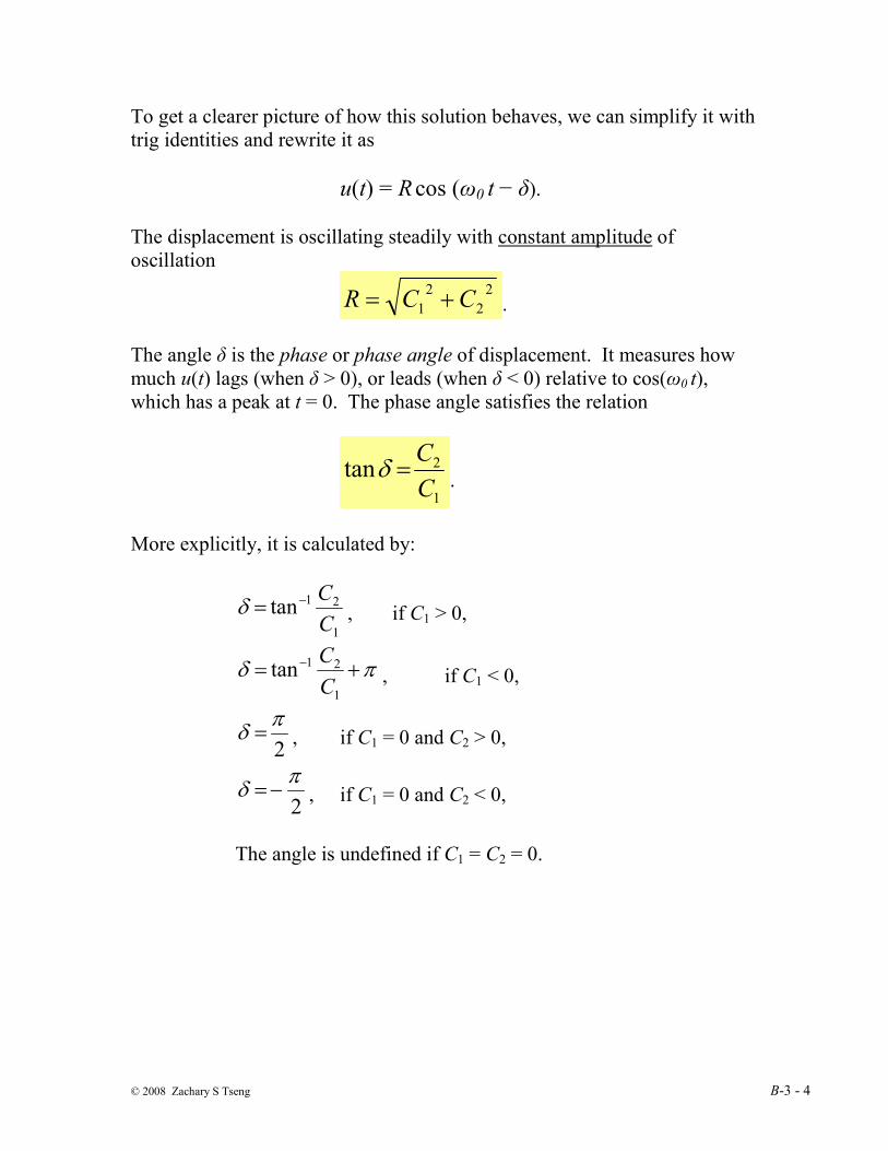
To get a clearer picture of how this solution behaves, we can simplify it with

trig identities and rewrite it as

u(t) = R cos (ω0 t − δ).

The displacement is oscillating steadily with constant amplitude of

oscillation

2

2

2

1 CCR += .

The angle δ is the phase or phase angle of displacement. It measures how

much u(t) lags (when δ > 0), or leads (when δ < 0) relative to cos(ω0 t),

which has a peak at t = 0. The phase angle satisfies the relation

1

2tanC

C=δ

.

More explicitly, it is calculated by:

1

21tanC

C−=δ , if C1 > 0,

πδ += −

1

21tanC

C, if C1 < 0,

2

πδ = , if C1 = 0 and C2 > 0,

2

πδ −= , if C1 = 0 and C2 < 0,

The angle is undefined if C1 = C2 = 0.


An example of simple harmonic motion:

Graph of u(t) = cos(t) − sin(t)

Amplitude: 2=R

Phase angle: δ = −π/4


Damped Free Vibration (γ > 0, F(t) = 0)

When damping is present (as it realistically always is) the motion equation

of the unforced mass-spring system becomes

m u″ + γ u′ + k u = 0.

Where m, γ, k are all positive constants. The characteristic equation is m r2 +

γ r + k = 0. Its solution(s) will be either negative real numbers, or complex

numbers with negative real parts. The displacement u(t) behaves differently

depending on the size of γ relative to m and k. There are three possible

classes of behaviors based on the possible types of root(s) of the

characteristic polynomial.

Case I. Two distinct (negative) real roots

When γ2 > 4mk, there are two distinct real roots, both are negative. The

displacement is in the form

trtreCeCtu 21

21)( += .

A mass-spring system with such type displacement function is called

overdamped. Note that the system does not oscillate; it has no periodic

components in the solution. In fact, depending on the initial conditions the

mass of an overdamped mass-spring system might or might not cross over

its equilibrium position. But it could cross the equilibrium position at most

once.


Figures: Displacement of an Overdamped system

Graph of u(t) = e−t

− e−2t

Graph of u(t) = − e−t

+ 2e−2t


Case II. One repeated (negative) real root

When γ2 = 4mk, there is one (repeated) real root. It is negative:

mr

2

γ−= .

The displacement is in the form

u(t) = C1 e rt + C2 t e rt.

A system exhibits this behavior is called critically damped. That is, the

damping coefficient γ is just large enough to prevent oscillation. As can be

seen, this system does not oscillate, either. Just like the overdamped case,

the mass could cross its equilibrium position at most one time.

Comment: The value γ2 = 4mk → mk2=γ is called critical damping. It

is the threshold level below which damping would be too small to prevent

the system from oscillating.


Figures: Displacement of a Critically Damped system

Graph of u(t) = e−t / 2

+ t e− t / 2

Graph of u(t) = e−t / 2

− t e− t / 2


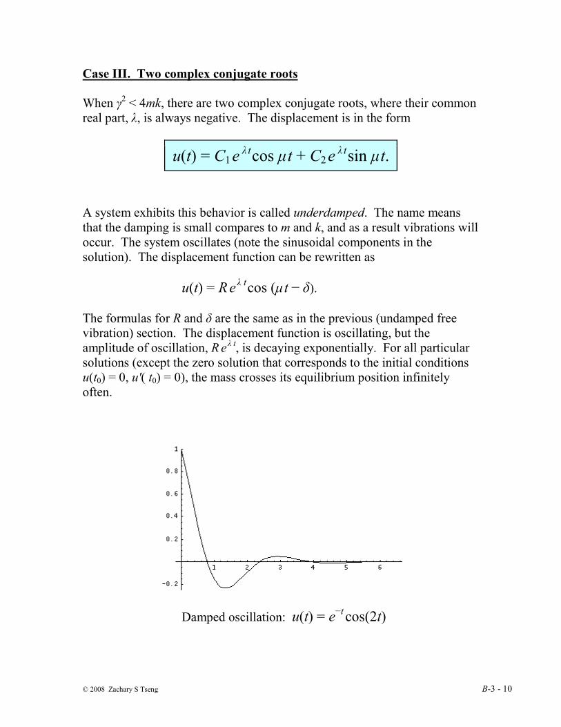
Case III. Two complex conjugate roots

When γ2 < 4mk, there are two complex conjugate roots, where their common

real part, λ, is always negative. The displacement is in the form

u(t) = C1 e λ t

cos µ t + C2 e λ t

sin µ t.

A system exhibits this behavior is called underdamped. The name means

that the damping is small compares to m and k, and as a result vibrations will

occur. The system oscillates (note the sinusoidal components in the

solution). The displacement function can be rewritten as

u(t) = R e λ t

cos (µ t − δ).

The formulas for R and δ are the same as in the previous (undamped free

vibration) section. The displacement function is oscillating, but the

amplitude of oscillation, R e λ t

, is decaying exponentially. For all particular

solutions (except the zero solution that corresponds to the initial conditions

u(t0) = 0, u′( t0) = 0), the mass crosses its equilibrium position infinitely

often.

Damped oscillation: u(t) = e−t

cos(2t)


The displacement of an underdamped mass-spring system is a quasi-periodic

function (that is, it shows periodic-like motion, but it is not truly periodic

because its amplitude is ever decreasing so it does not exactly repeat itself).

It is oscillating at quasi-frequency, which is µ radians per second. (It’s just

the frequency of the sinusoidal components of the displacement.) The peak-

to-peak time of the oscillation is the quasi-period: µπ2

=qT (seconds).

In addition to cause the amplitude to gradually decay to zero, damping has

another, more subtle, effect on the oscillating motion: It immediately

decreases the quasi-frequency and, therefore, lengthens the quasi-period

(compare to the natural frequency and natural period of an undamped

system). The larger the damping constant γ, the smaller quasi-frequency and

the longer the quasi-period become. Eventually, at the critical damping

threshold, when mk4=γ , the quasi-frequency vanishes and the

displacement becomes aperiodic (becoming instead a critically damped

system).

Note that in all 3 cases of damped free vibration, the displacement function

tends to zero as t → ∞. This behavior makes perfect sense from a

conservation of energy point-of-view: while the system is in motion, the

damping wastes away whatever energy the system has started out with, but

there is no forcing function to supply the system with additional energy.

Consequently, eventually the motion comes to a halt.


Example: A mass of 1 kg stretches a spring 0.1 m. The system has a

damping constant of γ = 14. At t = 0, the mass is pulled down 2 m and

released with an upward velocity of 3.5 m/s. Find the displacement function.

What are the system’s quasi-frequency and quasi-period?

m = 1, γ = 14, L = 0.1;

mg = 9.8 = kL = 0.1 k → 98 = k.

The motion equation is u″ + 14 u′ + 98 u = 0, and

the initial conditions are u(0) = 2, u′(0) = −3.5.

The roots of characteristic polynomial are r = −7 ± 7i:

u(t) = C1 e −7

t cos 7 t + C2 e

−7 t sin 7 t

Therefore, the quasi-frequency is 7 (rad/sec) and the quasi-period is

7

2π=qT (seconds).

Apply the initial condition and we get C1 = 2, and C2 = 3/2. Hence

u(t) = 2e −7t

cos 7 t + 1.5e −7t

sin 7 t.


Summary: the Effects of Damping on an Unforced Mass-Spring System

Consider a mass-spring system undergoing free vibration (i.e. without a

forcing function) described by the equation:

m u″ + γ u′ + k u = 0, m > 0, k > 0.

The behavior of the system is determined by the magnitude of the damping

coefficient γ relative to m and k.

1. Undamped system (when γ = 0)

Displacement: u(t) = C1 cos ω0 t + C2 sin ω0 t

Oscillation: Yes, periodic (at natural frequencym

k=0ω )

Notes: Steady oscillation with constant amplitude2

2

2

1 CCR += .

2. Underdamped system (when 0 < γ2 < 4mk)

Displacement: u(t) = C1 e λ t

cos µ t + C2 e λ t

sin µ t

Oscillation: Yes, quasi-periodic (at quasi-frequency µ)

Notes: Exponentially-decaying oscillation

3. Critically Damped system (when γ2 = 4mk)

Displacement: u(t) = C1 e rt

+ C2 t e rt

Oscillation: No

4. Overdamped system (when γ2 > 4mk)

Displacement: trtr

eCeCtu 21

21)( +=

Oscillation: No


Critically Damped

No Oscillation Displacement: u(t)= C1 e

rt + C2 te

rt

Mass crosses equilibrium at most once.

Mechanical Vibrations, F(t) = 0

Underdamped

System oscillates with amplitude decreasing

exponentially overtime,

Displacement: u(t)= C1eλt

cos µt + C2 eλt

sin µt,

Oscillation quasi periodic: Tq = 2π/µ

Overdamped

No Oscillation,

Displacement: u(t)= C1 e r1 t

+ C2 e r2 t

,

Mass crosses equilibrium at most once.

γ

Undamped γ = 0, Displacement: u(t)= C1 cos ω0t + C2 sin ω0t

Natural frequency: ω0 = , Steady oscillation with constant amplitude

γ2 > 4mk

γ=0

γ2 = 4mk

γ2 < 4mk

DA

MP

ING

IN

CR

EA

SE

S


Forced Vibrations

Undamped Forced Vibration (γ = 0, F(t) ≠ 0)

Now let us introduce a nonzero forcing function into the mass-spring system.

To keep things simple, let damping coefficient γ = 0. The motion equation is

m u″ + k u = F(t).

In particular, we are most interested in the cases where F(t) is a periodic

function. Without the losses of generality, let us assume that the forcing

function is some multiple of cosine:

m u″ + k u = F0 cos ωt.

This is a nonhomogeneous linear equation with the complementary solution

uc(t) = C1 cos ω0 t + C2 sin ω0 t.

The form of the particular solution that the displacement function will have

depends on the value of the forcing function’s frequency, ω.

Case I. When ω ≠ ω0

If ω ≠ ω0 then the form of the particular solution corresponding to the

forcing function is

Y = A cos ωt + B sin ωt.

Solving for A and B using the method of Undetermined Coefficients, we find

that tm

FY ω

ωωcos

)( 22

0

0

−= .

Therefore, the general solution of the displacement function is

tm

FtCtCtu ω

ωωωω cos

)(sincos)(

22

0

0

0201−

++= .


An interesting instance of such a forced vibration occurs when the initial

conditions are u(0) = 0, and u′(0) = 0. Applying the initial conditions to the

general solution and we get

)( 22

0

0

1ωω −

−=

m

FC , and C2 = 0.

Thus,

( )ttm

Ftu 022

0

0coscos

)()( ωω

ωω−

−= .

Again, a clearer picture of the behavior of this solution can be obtained by

rewriting it, using the identity:

sin(A) sin(B) = [cos(A − B) − cos(A + B)] / 2.

The displacement becomes

2

)(sin

2

)(sin

)(

2)(

00

22

0

0 tt

m

Ftu

ωωωω

ωω

+

−

−= .

The behavior exhibited by this function is that the higher-frequency, of

(ω0 + ω) / 2, sine curve sees its amplitude of oscillation modified by its

lower-frequency, of (ω0 − ω) / 2, counterpart.

This type of behavior, where an oscillating motion’s own amplitude shows

periodic variation, is called a beat. The quantity ωb = | ω0 – ω | is called the

beat frequency. It can be derived by dividing 2π by the distance between

adjacent zeros of 2

)(sin

0 tωω −.


An example of beat:

Graph of u(t) = 5 sin(1.8t) sin(4.8t)


Case II. When ω = ω0

If the periodic forcing function has the same frequency as the natural

frequency, that is ω = ω0, then the form of the particular solution becomes

Y = A t cos ω0 t + B t sin ω0 t.

Use the method of Undetermined Coefficients we can find that

A = 0, and 0

0

2 ωm

FB = .

The general solution is, therefore,

ttm

FtCtCtu 0

0

0

0201 sin2

sincos)( ωω

ωω ++=

.

The first two terms in the solution, as seen previously, could be combined to

become a cosine term u(t) = R cos (ω0 t − δ), of steady oscillation. The third

term, however, is a sinusoidal wave whose amplitude increases

proportionally with elapsed time. This phenomenon is called resonance.

Resonance: graph of u(t) = t sin(t)


Technically, true resonance only occurs if all of the conditions below are

satisfied:

1. There is no damping: γ = 0,

2. A periodic forcing function is present, and

3. The frequency of the forcing function exactly matches the

natural frequency of the mass-spring system.

However, similar behaviors, of unexpectedly large amplitude of oscillation

due to a fairly low-strength forcing function occur when damping is present

but is very small, and/or when the frequency of forcing function is very

close to the natural frequency of the system.


Exercises B-3.1:

1 – 4 Solve the following initial value problems, and determine the natural

frequency, amplitude and phase angle of each solution.

1. u″ + u = 0, u(0) = 5, u′(0) = −5.

2. u″ + 25u = 0, u(0) = −2, u′(0) = 310 .

3. u″ + 100u = 0, u(0) = 3, u′(0) = 0.

4. 4u″ + u = 0, u(0) = −5, u′(0) = −5.

5 – 10 Solve the following initial value problems. For each problem,

determine whether the system is under-, over-, or critically damped.

5. u″ + 6u′ + 9u = 0, u(0) = 1, u′(0) = 1.

6. u″ + 4u′ + 3u = 0, u(0) = 0, u′(0) = −4.

7. u″ + 6u′ + 10u = 0, u(0) = −2, u′(0) = 9.

8. u″ + 2u′ + 17u = 0, u(0) = 6, u′(0) = −2.

9. 4u″ + 9u′ + 2u = 0, u(0) = 3, u′(0) = 1.

10. 3u″ + 24u′ + 48u = 0, u(0) = −5, u′(0) = 6.

11. Consider a mass-spring system described by the equation

2u″ + 3u′ + k u = 0. Give the value(s) of k for which the system is under-,

over-, and critically damped.

12. Consider a mass-spring system described by the equation

4u″ + γ u′ + 36u = 0. Give the value(s) of γ for which the system is under-,

over-, and critically damped.

13. One of the equations below describes a mass-spring system undergoing

resonance. Identify the equation, and find its general solution.

(i.) u″ + 9u = 2cos 9t (ii.) u″ + 4u′ + 4u = 3sin 2t

(iii.) 4u″ + 16u = 7cos 2t


14. Find the value(s) of k, such that the mass-spring system described by

each of the equations below is undergoing resonance.

(a) 8u″ + k u = 5sin 6t (b) 3u″ + k u = −π cos t

Answers B-3.1:

1. u = 5cos t − 5sin t, ω0 = 1, R = 25 , δ = −π / 4

2. u = −2cos 5t + 32 sin 5t, ω0 = 5, R = 4, δ = 2π / 3

3. u = 3cos 10t, ω0 = 10, R = 3, δ = 0

4. u = −5cos t / 2 − 10sin t / 2, ω0 = 1 / 2, R = 55 , δ = π + tan−1

2

5. u = e −3t

+ 4t e −3t

, critically damped

6. u = 2e −3t

− 2e −t

, overdamped

7. u = −2e −3 t

cos t + 3e −3 t

sin t, underdamped

8. u = 6e − t

cos 4t + e − t

sin 4t, underdamped

9. u = 4e −t

/ 4 − e

−2t, overdamped

10. u = −5e −4t

− 14t e −4t

, critically damped

11. Overdamped if 0 < k < 9 / 8, critically damped if k = 9 / 8, underdamped

if k > 9 / 8.

12. Underdamped if 0 < γ < 24, critically damped if γ = 24, overdamped if

γ > 24. When γ = 0, the system is undamped (rather than underdamped).

13. (iii), tttCtCu 2sin16

72sin2cos 21 ++=

14. (a) k = 288 (b) k = 3

Mechanical Vibrations - Sites at Penn State · Mechanical Vibrations A mass m is suspended at the...

Documents

Transcript of Mechanical Vibrations - Sites at Penn State · Mechanical Vibrations A mass m is suspended at the...