Mechanical Vibrations Prof. S. K. Dwivedy Department of ... · about this Rayleigh method and...
41
Mechanical Vibrations Prof. S. K. Dwivedy Department of Mechanical Engineering Indian Institute of Technology, Guwahati Module - 10 Lecture -3 Approximate Solutions for Continuous and Discrete Systems Durkerley, Rayleigh-Ritz and Galerkin Method So, in the last 2 lecture, we are studying about this approximate method, to find the natural frequency of discrete and distributed mass systems. So, we have already studied about this Rayleigh method and matrix iteration method. (Refer Slide Time: 01:12) So, in Rayleigh principle tells in a conservative system the frequency of vibration has a stationary value in the neighborhood of the natural mode. So, in case of Rayleigh method we determine the Rayleigh quotient. So, which is given by this expression here Z is the approximate function we are taking or approximate mode. We are taking in case of discrete system, K is the stiffness matrix and M is the mass matrix of the system by taking this Rayleigh quotient. So, we can find the omega square or the frequency square of the frequency and we can find the frequency. Also we can equate the maximum kinetic energy to the maximum potential energy to find the fundamental frequency.
Transcript of Mechanical Vibrations Prof. S. K. Dwivedy Department of ... · about this Rayleigh method and...

Mechanical Vibrations
Prof. S. K. Dwivedy
Department of Mechanical Engineering
Indian Institute of Technology, Guwahati
Module - 10
Lecture -3
Approximate Solutions for Continuous and Discrete Systems
Durkerley, Rayleigh-Ritz and Galerkin Method
So, in the last 2 lecture, we are studying about this approximate method, to find the
natural frequency of discrete and distributed mass systems. So, we have already studied
about this Rayleigh method and matrix iteration method.
(Refer Slide Time: 01:12)
So, in Rayleigh principle tells in a conservative system the frequency of vibration has a
stationary value in the neighborhood of the natural mode. So, in case of Rayleigh method
we determine the Rayleigh quotient. So, which is given by this expression here Z is the
approximate function we are taking or approximate mode. We are taking in case of
discrete system, K is the stiffness matrix and M is the mass matrix of the system by
taking this Rayleigh quotient. So, we can find the omega square or the frequency square
of the frequency and we can find the frequency. Also we can equate the maximum
kinetic energy to the maximum potential energy to find the fundamental frequency.

(Refer Slide Time: 02:00)
And in the matrix iteration method, so this method is particularly useful for discrete
system. So, let us consider a n degrees of freedom system, the equation motion of the
system can be written by M x double dot plus K x equal to 0 or by taking the dynamic
matrix M inverse K. I can write this expression in this way that is AX equal to lambda X.
where lambda is equal to omega square lambda equal to omega square is the Eigen value
of the system and X is the mode shapes or Eigen vector of this system. So, from this any
normal mode, when for this you can observe that any normal mode, so let X is the
normal mode.
So, any normal mode when multiplied with this dynamics matrix you can see that it
repeat itself. So, this is basic principle of this matrix iteration method. So, by taking any
approximate mode, so when we are multiplying this with this dynamic matrix we will get
another vector. So, if you, will normalize that thing and check with the previous vector
or assumed vector. So, if it is not same we can continue that iteration and we can find the
mode or normal mode. So, after finding the normal mode we can obtain the natural
frequency of the system or we can obtain the value of lambda.

(Refer Slide Time: 03:27)
So, to obtain the higher mode, so we should apply the orthogonality principle because in
case of the free vibration response what we are taking it contains the first mode first
mode or first modal frequency. So, if you eliminate this first mode then only we can find
or the assumed solution will lead to the second mode. So, in this case let we take this free
vibration response or mode shape as X. So, this X can be written as a linear combination
of other modes. So, it can be written as c 1 X 1 plus C 2 X 2 plus C 3 X 3 and c n X n.
So, in this way I can write this X equal to this is the assumed mode. So, this assumed
mode X can be written in this form. X 1 bar X 2 bars X 3 bar for a 3 degrees for freedom
system. I have written this thing.
So, this X equal to X 1 bar X 2 bar X 3 bar transpose and this Xi these are normal modes.
So, these X 1 X 2 X 3 transpose. So, the normal mode this X 1 X 2 X 3 can be written
for a 3 degrees of freedom system like this and this is assumed mode. So, now applying
the orthogonality principle, so I can pre-multiply X transpose M in this equation. So, in
the first equation when pre-multiplying these X transpose M I have X transpose M x
equal to c 1 into X 1 transpose MX 1 plus c 2 into X 1 transpose M x 2 and plus c 3 into
X 1 transpose M x 3. And similarly, you can find this is equal to plus c n X 1 transpose
M x n. So, from the orthogonality principle you know that Xi transpose M x j. So, this is
equal to 0 when I not equal j.

So, when I not equal to j from orthogonality principle we know that Xi transpose M X j
equal to 0. So, this c 2, so this X 1 dashed X 1 transpose MX 2 equal to 0. So, this part
equal to part to 0 and other times all other terms except this X 1 transpose MX 1 equal to
0. So, this X 1 transpose MX 1 equal to. So, if I am taking this X 1 as a normalized
vector then it will be equal to 1. So, or it can be written as c 1 X 1 transpose MX 1. So,
these term will remain and other terms will be 0. So, this X 1 transpose MX will be equal
to c 1 X 1 transpose MX 1. So, now to eliminate the first mode we should put the c 1
equal to 0. So, putting c 1 equal to 0 the left hand side of this equation becomes 0.
(Refer Slide Time: 06:29)
So, the left hand side of this equation that is equal to X 1 dash MX equal to 0. Now, for
the 3 degrees freedom system I can substitute these in this way. So, X 1 dash equal X 1
X 2 X 3 and this is mass matrix and this is these assumed mode. So, assumed I have
taken as X 1 bar X 2 bar X 3 bar. So, by multiplying this thing you can get this equation
that is M 1 X 1 X 1 bar plus M 2 X 2 X 2 bar plus M 3 X 3 X 3 bar equal to 0. So, in this
case I can express these X 1 bar in terms of X 2 bar and X 3 bar. So, X 1 bar I have
written equal to minus M 2 by M 1 X 2 by X 1 into X 2 bar minus M 3 by M 1 into X 3
by X 1 into X 3 bar, and I can write other 2 expression that is X 2 bar equal to X 2 bar
identity. So, these are identity equation. So, this is X 3 bar equal to X 3 bar. So, I can
write these 3 expression in a matrix form.

(Refer Slide Time: 07:35)
So, that matrix will be equal to X 1 bar X 2 bar X 3 bar equal to. So, 0 minus M 2 by M
1 X 2 by X 1 minus M 3 by M 1 X 3 by X 1 then 0 1 0 0 0 0. So, you can note that the
first column of this matrix equal to 0. So, this first column equal to 0. So, as the first
column equal to 0, if you multiply this matrix or if you take this matrix. So, it will sweep
out the first mode from the assumed vibration. So, this matrix is known as the sweeping
matrix S. So, this matrix is known as the sweeping matrix. So, using the sweeping
matrix, so we can find or we can eliminate the first mode from the resulting vibration.
Similarly, to eliminate the second mode we can put c 2 equal to 0 and for third mode c 3
equal to 0. So, when you are eliminating first 2 modes we should put c 1 and c 2 equal to
0 and applying this orthogonality principle, we can find the sweeping matrix
corresponding to the second mode third mode or higher modes. So, by eliminating these
modes from the assumed vibration, then our iteration process will converse to the higher
modes.

(Refer Slide Time: 08:57)
So, let us take 1 example to study this thing. So, let this is a beam or this is a rod with 3
masses and this is vibrating in this transverse direction. So, the vibration is taking place
in this transverse direction. So, this mass is 3 M and this mass is 2 M and this mass is M.
So, the you can think of a tall building with mass 3 M concentrated here, 2 M
concentrated here and M concentrated here these are the mass of the roof and these are
the stiffness of the walls. So, these stiffness the first part it is 4 k second part I have taken
it equal to 2 k and the third part it is equal to k. So, due to this wind motion, so it may
vibrate in this transfer direction. So, we have to study or we have to find the first 3
natural frequency of the system due to this vibration to find this. So, first we have to find
the stiffness matrix, mass matrix.
So, mass matrix is simple and mass matrix you can write in this way. So, the max matrix
will be equal to. So, this is X 1 I am taking this vibration X 1 this is X 2 and this is X 3.
So, this is the first mass I am taking this is the second mass and this is the third mass. So,
in this case, so I can write this 3 M 0 0 0 2 M 0 and 0 0 0 0 0 M. So, this is the mass
matrix and to find this stiffness matrix, or we can proceed in the other way that is we can
find the flexibility matrix. And by finding the flexibility matrix also we can find the
equation motion, and from that equation motion we can proceed. So, to find the
displacement, so a 1 1 that is influence coefficient let us first find the influence
coefficient. The influence coefficient a 1 1, that is displacement at 1 due to unit force at 1
while the forces at other places are 0.

So, as there is no force acting at these 2 places and only force acting at this place is equal
unity force. So, these part will give resistance to its motion, as this part has a stiffness of
4 k. So, the displacement will be 1 by 4 k. So, a 1 1 equal to 1 by 4 k, so as there is no
force acting at this 2 and 3. So, a 1 a 2 1 that is displacement at 2 due to a unit force at 1
will be same as the displacement of this position. That means, the beam will bend from
this position and it will be straight at these 2 position. So, the displacement here it will be
1 by 4 k and also the displacement here will be 1 by 4 k and the displacement here will
be 1 by 4 k, so this displacement. So, this influence coefficient are written like this a 1 1
equal to a 2 1 equal to a 3 1 equal to 1 by 4 k. Similarly, let us find.
So, we can find this a 2 2. So, applying a force at 2 unit force at 2 and no force at 3 and 1
we can find this influence coefficient a 2 2. So, a 2 2, so while finding a 2 2. So, these
stiffness and these stiffness will be coming into picture. So, these 2 are in series. So, the
resulting or equivalent stiffness will be 1 by 4 k plus 1 by 2 k. So, this is 1 by 4 k plus 1
by 2 k that is equal to 3 by 4 k. So, the displacement will be equal to 3 by 4 k, so a 2 2
equal to 3 by 4 k. So, when it is displaced to this position let it is coming to this position
due to the unit force here. So, the upper portion also will have the same motion as there
is no force acting at 3. So, this a 3 2 also will be same as that of a 2 2 and applying the
reciprocity theorem also you know a I j equal to a j I that is a displacement at I. Due to a
unit force at j equal to a displacement at j due to a unit force at I that is the reciprocity
theorem.
So, applying that theorem you can write a 2 2 equal to a 2 3 equal to a 3 2 equal to 3 by 4
k. Similarly, here a 1 1 already you know that this a 1 1 equal to a 2 1 equal to a 3 1. So,
by applying reciprocity theorem a 2 1 equal to a 1 2 similarly a 3 1 equal to a 1 3, so this
is equal to 1 by 4 k. Now, to obtain this a 3 3, so we can apply a unit force at 3 and no
force at 2 1 1. So, when we are applying a unit force here at 3. So, this part this part these
3 parts will give resistance to its motion. So, these 3 stiffnesses are in series, so the net
stiffness or net equivalent stiffness will be equal to 1 by 1 by k will be equal to 1 by 4 k
plus 1 by 2 k plus 1 by 2 k plus 1 by k. So, 1 by k equivalent will be equal to 1 by 4 k 1
by 2 k plus 1 by k. So, the net or the deflection of this 3 will be equal to 1 by 4 k plus 1
by 2 k plus 1 by k that is equal to 7 by 4 k, so a 3 3 equal to 7 by 4 k.

(Refer Slide Time: 14:49)
So, the flexibility matrix I can write it in this form. So, a will be equal to 1 by 4 k 1 1 1 1
3 3 and 3 3 7 and the mass matrix already I have written. So, that is equal to 3 0 0 0 2 0
and 0 0 1 into m. So, the hence the displacement at these position now actually at these
positions this inertia forces are acting. So, the displacement at these position due to this
actual forces that is here it will be 3 m into omega square with a negative sign, here 2 m
into omega square and here m into omega square with negative sign So, as inertia force
act in the opposite direction to the displacement. We have this negative sign in 3 places,
and the displacement here will be equal to displacement at position 1.
So, the displacement at position 1 will be equal to a 1 1 into the force at 1 similarly a 1 2
into the force at 2 and a 1 3 into the force at 3. So, as a I j equal to displacement at I due
to unit force at j. So, due to these inertia forces at these positions, so you can find the net
displacement at position 1 equal to a 1 1 into 3 into m x 1 double dot plus a 1 2 into 2
into m x 2 double dot a 1 3 into m x 3 double dot. So, due to inertia forces it acts
opposite to the direction of displacement that is why the negative sign is given here.
Similarly, x 2 will be equal to a 2 1 into the force acting at 1 that is 3 m x double dot and
a 2 2 into force acting at 2 that is equal to 2 m that this is mass and acceleration is x 2
double dot and a 2 3 into m into x 3 double dot.
Similarly, x 3 will be equal to minus a 3 1 4. So, this is equal to 3 3 m x 1 double dot
plus a 3 2 2 into m x 2 double dot and a 3 3 into m x 2 double dot. So, these are the

inertia forces and multiply it with this mass this is the x 3 double dot or x 1 double dot x
2 double as acceleration multiplied by the mass of the that location will give the inertia
force and the inertia force acts in a direction opposite to the direction of displacements.
So, in this way you can find the displacement x 1 x 2 x 3.
(Refer Slide Time: 17:38)
So, the displacement x 1 x 2 x 3 after substituting this xi double dot equal to minus
omega square xi and we can write this x 1 x 2 x 3 equal to m omega square by 4 k 3 2 1 3
6 3 12 6 7 and x 1 x 2 x 3. So, this is the equation iterative equation, which we will use to
find the frequency of the system. So, let us take some value of x 1 x 2 x 3 and see what is
happening or what we are getting. So, I will show you the simulation now. So, let me
show the simulation by using this matlab.

(Refer Slide Time: 18:19)
So, I can write this matrix let me take this matrix at c matrix. So, this c matrix equal to I
can write this. So, this is equal to 3 2 1. So, this is 3 this is 2 and 1 3 2 1 then 3 3 6 3 2 1
3 6 3 3 then 6 then 3 and 3 6 7 3 6 and 7.
(Refer Slide Time: 19:05)
So, this matrix you can see will be equal to. So, this is the matrix I have taken that is 3 2
1 3 6 3 and 3 6 7. Now, in this matrix, so I have to multiply I have to multiply 1 assumed
mode. So, let me take the assumed mode let us take any arbitrary assumed mode. So, let
me take it equal to 1 2 3. So, the trial function let me take this trial function t equal to.
So, the trail function I can take equal to. So, this is equal to 1 2 3 I will take. So, this is 1
2 and 3. So, I will take the transpose of this. So, this is the trail function.
(Refer Slide Time: 19:52)
So, this trial function equal to 1 2 3. So, I have to multiply these trial function with the
previous function that is c. So, let me find let I am writing e equal to c multiplied by this.
(Refer Slide Time: 20:15)
So, I can write e equal to c.
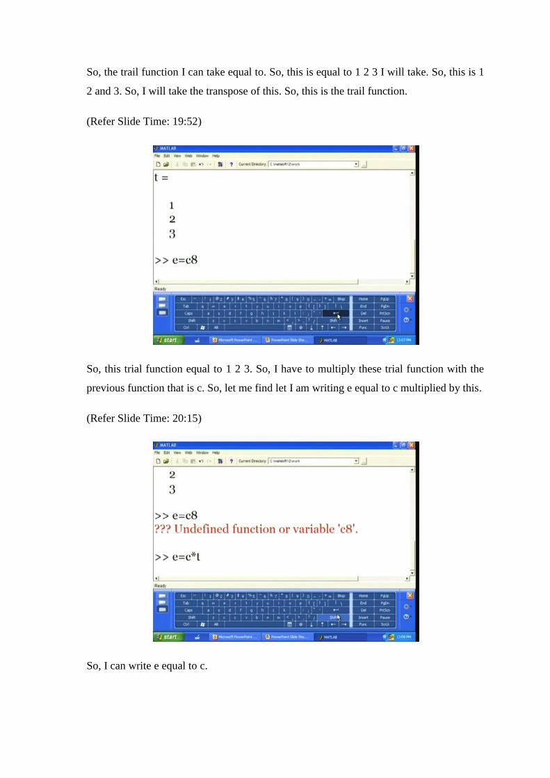
(Refer Slide Time: 20:30)
So, by multiplying the c into t, so we are getting this vector that is 10 24 and 36. Now, I
can normalize this vector that is this 10 had 24 and 36. So, I can normalize it by dividing
this 36 in this, so by to divide this thing by 36. So, let me write this t. So, this thing will
be my x or the next x for next iteration. So, x will be equal to t by this e or t by 36 let me
directly write, so t by 36.
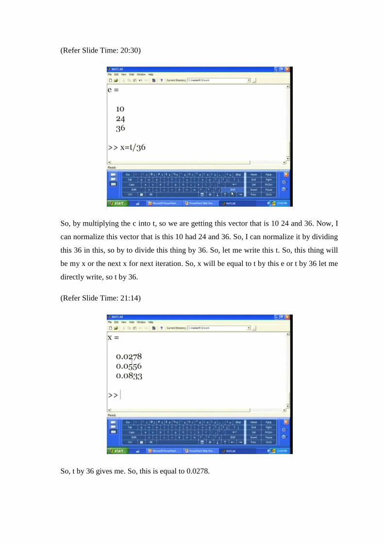
(Refer Slide Time: 21:14)
So, t by 36 gives me. So, this is equal to 0.0278.

(Refer Slide Time: 21:19)
So, this value you can see.
(Refer Slide Time: 21:20)
So, this is equal to 10 24 and 36. So, x will be equal to. So, this is the function e. So, by e
I have to divide this 36 to get this normal mode.

(Refer Slide Time: 21:35)
So, this will be. So, I can write x equal to e by. So, this is e by 36 not t by 36.
(Refer Slide Time: 21:44)
So, e by 36 will give me 0.2778, 0.6667 and 1. So, this is the normalized value, I will
take for next iteration. So, you can note that this value is not equal to the value we have
assumed that is we have assumed a value equal to. So, we have assumed this value 1 2 3
and by putting that thing in this equation we are getting a value equal to 0.2778, 0.6667
and 1. So, now for next iteration I will take this value and multiply this with the c value.,

so c. So, next iteration I can write c into. So, I can write let s equal to or e equal to e
equal to c into c into this x. So, I will multiply this thing.
(Refer Slide Time: 22:44)
And I am a getting a value this e equal to this and normalize this thing I can use this e by.
So, I will half this trail function again will be equal to c divided by this 11 that is e 3. So,
I can write e in bracket 3 also I can write or I can write this is equal to 11.833.
(Refer Slide Time: 23:19)
So, by dividing this thing I will get the value. So, I have to. So, this is the value of e I
obtain, so in this e. So, trail value I have to normalize this. So, I have to divide this e by

11 this thing. So, it will be. So, this t will be equal to t will be equal to e by. So, it will be
equal to e by 11. So, you can see this thing. So, this is equal to 11.8333. So, 8333.
(Refer Slide Time: 24:06)
So, dividing this thing, so we are normalizing these under normalized value is now
0.2676 and 0.6620 and 1.
(Refer Slide Time: 24:21)
So, you have taken a trial function that is equal to. So, the trial function what we have
taken. So, this is equal to 0.2778, 0.6667 and 1 and you are getting the function equal to
0.2676, 0.6620 and 1. So, in this way you can take this as the, for next iteration, you can

take this function this mode you can take and you can proceed and finally, you will find
the value for which both side will be same. So, let me take the final value. So, what I
obtained. So, t trial function if you take t equal to. So, let me take this trial function equal
to t equal to 1 2.4895 and then 3.7738. So, taking these as the trial function, so let this is
taken as the trial function.
(Refer Slide Time: 25:31)
So, this is the trial function we have taken that is equal to 1 2.4895 and this. So, let me
multiply this with c. So, let x I am writing x equal to c multiplied by. So, c multiplied by
this t.

(Refer Slide Time: 25:52)
So, c multiplied by t will give me this is the value I am getting. So, by normalizing this
thing, so by normalizing this thing I can write I will get this answer by dividing this x by.
So, I am normalizing with respect to this first 1 in this case because in the first 1 I have
put it equal to 1. So, I put this is equal to 11.7528. So, this will give the value 1 2.4895,
3.7739. So, you just note the trial function taken was 1 2.4895, 3.7738 and you are
getting the value also same 1 2.4895, 3.7739. So, this, so up to third decimal you are
getting the value accurately. So, in this way you can do the iteration to get. So, this is the
first mode. So, in this way you can get this first mode value that is equal to 1 2.4895 and
3.7739.

(Refer Slide Time: 27:00)
So, we got the first mode equal to 1 2.4895, 3.7738. So, when I multiply it. So, I can
write this equal to 1 2.4893, 3.7735 equal to 11.7521 m omega square by 4 k equal to
same. So, you can note this left hand side and right hand side. So, this is the assumed
mode we have taken, and this is the mode we obtained that is equal to x 1. So, in both the
sides you can note that you are getting up to third decimal accurate thing. So, when this
is equal to this then this part will be equal to 1. So, this is the first mode value and you
can get this equal to 1.
(Refer Slide Time: 27:47)

So, 11.7521 m omega square by 4 k. So, we equate to 1. So, in that way you can get the
first mode frequency that is equal to omega 1 square. So, this is equal to 0.3404 k by m
or omega 1 you can find root over of this and to find the second mode we can proceed
we have to find the sweeping matrix. Already we have found the sweeping matrix for the
first mode. So, we have to make c 1 equal to 0 in this assumed mode. to make c 1 equal
to 0. So, we have to write the sweeping matrix.
(Refer Slide Time: 28:24)
So, in this sweeping matrix already we got these x 2 x 1. So, this is the x 1 this is x 2 and
x 3 for the first mode. So, substituting this x 1 x 2 x 3 for the first mode equal to these,,
so we can write the sweeping matrix in this form. So, after getting the sweeping matrix,
so I can substitute it in this expression that is x equal to m omega square by 4 k into this
matrix into the sweeping matrix into x. So, this is the sweeping matrix and this is this is
the a matrix that is flexibility matrix into these mass matrix. This matrix is flexibility
matrix into mass matrix this is the sweeping matrix. So, this equation reduces to this.

(Refer Slide Time: 29:09)
So, x 1 x 2 x 3 equal to m omega square by 4 k into this matrix into x 1 x 2 x 3. So, you
can note that in the first column all the terms are 0. So, now any assumed value of x 1 x 2
x 3 will not go to the first mode and you will get the next higher mode that is the second
mode. So, let us start with any arbitrary value. So, proceed in the same way as I have
shown in this iteration before. So, by proceeding in the same way you can find the value
to be this. So, this will. So, this is the x you can when you are assuming x equal to
1.8367 minus 1.8996. So, you are getting a value that is equal to 1.8361 minus 1.899
8988. So, up to the second decimal you can see both are matching. So, you can take this
value and now. So, this will be equal to 1.

(Refer Slide Time: 30:22)
So, equating this middle part equal to 1 or the coefficient of this x equal to 1 you can find
this second mode frequency that is lambda 2 equal to 1.4411 k by m. So, omega 2 will be
equal to 1.2 root over per k by m. So, in this way you can get the second mode and this is
the second mode this is the second mode shape. So, x 2 is the modal matrix for the
second mode and omega 2 is the frequency of the second mode that is 1.2 into root over
k by m.
(Refer Slide Time: 30:52)

So, to obtained the third mode. So, we should set the c 1 and c 2 both equal to 0. So, to
set c 1 equal to 0 already we have derived this expression that is summation mi xi xi bar
equal to 0. So, for the 3 mode you can write this is equal to m 1 x 1 x 1 bar equal to m 1
x 1 x 1 bar plus m 2 x 2 x 2 bar plus m 3 x 3 x 3 bar equal to 0. Similarly, for c 2 equal to
0 I can write m 1 x 2. So, these x, so this is nothing but the x 2 we obtained just now and
this is the x 1 we obtained before. So, this is the x 1 of the first mode that is modal matrix
of the first mode this is the modal matrix of the second mode. So, substituting these
value. So, we can write the c 1 equal to this that is 3 x 1 bar plus 4.979 x 2 bar plus this
and c 2 equal to this.
(Refer Slide Time: 31:52)
So, after getting these 2 expression I can write x 1 bar in terms x 3 and x 2 bar also in
terms of x 3. So, you can write this x 1 bar x 2 bar x 3 bars equal to 0 0 1.5896, 0 0
minus 1.7157 and 0 0 1 x 1 bar x 2 bar x 3 bar. So, you can note that in this matrix the
first 2 columns are 0. So, if you multiply this matrix or you take this matrix and insert in
the original equation. So, the any vibration or any mode you supply that will eliminate
the first 2 modes. So, this matrix is known as the sweeping matrix for the second mode.
So, using the sweeping matrix, we can eliminate these first 2 modes now.

(Refer Slide Time: 32:44)
So, now substituting this in this equation, so this is your a into m matrix and this is the
sweeping matrix just now we have developed that is S 2. So, I can write m omega square
by 4 k into these into this S 2 into this. So, in the left hand side you just see this is x 1 x 2
x 3 equal to m by omega square by 4 k into this matrix into x 1 x 2 x 3. So, in the left
hand side, so by taking any assumed value x 1 x 2 x 3 we will determine this x 1 x 2 x 3
the iteration process we will continue till we are not getting the same value in the left
hand side and right hand side for x 1 x 2 x 3. So, but for this case immediately you can
see that this third column third column will be the x 3.
(Refer Slide Time: 33:41)

So, if you substitute this third column in this expression you can check and normalize
that thing. You can find that the value x 3 equal to 1.5896 minus 1.7157 and 1. So,
substituting this x 3 value you can find this 1.4746 m omega square by 4 k. So, this part
is not there. So, this is equal to 1. So, 1.47, so you can get 1.4 1.4746 m omega square by
4 k equal to 1.
(Refer Slide Time: 34:20)
So, from this you can get this omega square. So, that correspond to the third mode
frequency. So, in this way you can obtain the third mode frequency of the system. So, by
using this matrix iteration method in this way you can determine the mode shapes of
different modes, and the Eigen values or the frequency of the system.

(Refer Slide Time: 34:42)
So, let us now. So, same thing you can verify by writing the equation motion. The
equation motion can be written this is the mass matrix, and inverse of the flexibility
matrix will give the stiffness matrix and this is equal to 0. So, now you can find the
dynamic matrix that is m inverse k. So, this is the dynamic matrix by using the Eigen
value of this you can find the values are coming to be this. So, you can check that these
values and the values you obtained are same.
(Refer Slide Time: 35:14)

So, let us now see some other methods that is 1 methods is Dunkerley method. In
Dunkerley method you can find the natural frequency of a system when several masses
are acting on the system. So, let this is the, this is a simply supported beam. So, on this
beam let n number of loads are acting. So, these are the n number of loads acting on this
beam. So, due to this let this is the static deflection. So, we can find let this is equal to y
1 this y 2 and similarly this is equal to y n. So, let these are the deflection due to the load
acting at these positions. So, Dunkerley method give an approximate method or give an
approximation to find the fundamental frequency of the system.
So, in this case the frequency of the system that is equal to omega n you can find by
finding the natural frequency due to each load. So, first we have to find the natural
frequency due to each load and after getting the natural frequency from each for each
case, we can use this formula to find the natural frequency of the whole system. So, here
1 by omega n square, so omega n is the natural frequency of the system. So, omega n is
the natural omega n is the frequency of the system when only this load is acting on the
system. Similarly, omega n 2 is the frequency when only this frequency or only this load
is acting on the system.
Similarly, omega n 5 will be when this fifth load is acting only if you find the frequency
of the system, then that will be omega n and omega S the last 1 is the omega S. So,
omega S is the natural frequency of the system when no load is acting on the system, but
the mass of the system is considered that is a uniformly distributed load of this beam is
considered. So, the total, so 1 by omega n square equal to 1 by omega n a square plus 1
by omega n 1 square plus 1 omega n 2 square. And similarly, you can add till the last
mass is considered, so by taking all the frequencies. So, you can use this formula to find
the natural frequency of the, of a complex system.

(Refer Slide Time: 37:58)
So, let us take 1 example. So, let this is a simply supported beam. So, in this simply
supported beam we have taken 3 masses. So, this middle mass we have taken equal to 2
m and this side mass equal to m 1 and this mass equal to m. So, this is m 1. So, we have
taken this and first mass and last mass same and the second mass we have taken equal to
twice of the first mass. So, in this case we have to find the natural frequency of the
system we have not considered the mass of the beam, so without considering the mass of
the beam. So, we here we can find the natural frequency or the frequency due to this
mass frequency due to this mass and frequency due to this mass individually.
And then we can use this formula 1 by omega m square equal to 1 omega 1 square plus 1
by omega 2 square and plus 1 by omega 3 square and we can find the natural frequency.
So, to find that thing let us first find the flexibility influence coefficient that is the
displacement at these points. After getting these displacement, we can find the natural
frequency as omega n will be equal to root over g by delta. So, first we can find these
displacement due to these mass at this position. So, a 1 1 is the displacement at 1 due to a
unit force at 1. So, when unit force is applied at these position. So, we can find the
displacement will be equal to 3 l cube by 2 56 EI. Similarly, we can find when only this
mass is present. So, if you put a unit a unit force here the displacement will be l cube by
48 EI. So, you know for a simply supported beam at the.

So, when it is loaded at the middle the displacement equal to w l cube by 3 I. So, now by
putting this weight equal to. So, at the middle when it is loaded at the middle the
displacement equal to w it w l cube by 48 EI. So, now by putting w equal to 1. So, you
are getting this is equal to l cube by forty-eight EI. Similarly, a 3 1 you can find. So, a 1
1 a 2 2 a 3 3 that is displacement at 1 due to unit displacement at 1 due to unit force at 1
displacement at 2 due to unit force at 2 and displacement at 3 due to unit force at 3. So,
in this way you can obtain.
(Refer Slide Time: 40:30)
So, after obtaining this thing, so you can write 1 by omega 1 square will be equal to. So,
root over g by delta omega. So, 1 by omega 1 square will be equal to 3 ml cube by 256
EI. So, you can divide these things, so g by this. So, you can find the terms like this. So,
2 ml cube by this and this is equal to 1 by omega square equal to 2 ml cube by 48 EI and
1 by omega 3 square equal to 3 w l cube by 256 EI. So, this is equal to g by. So, we have
put only these. So, in this case we have just divided by g as this weight 1 Newton was
taken. So, this is equal to mass of 1 into g.
So, this will be mg for a load of m. So, the displacement will be equal to a load of w the
displacement will be equal to w into l cube by 256 EI. So, by dividing this by g as this
omega n equal to or omega n square equal to g by delta you can find. So, this will give g
by delta. So, delta equal to here 3 w l cube by 256 EI. So, g by delta will give w equal to
mg. So, substituting w equal to mg you can find this expression. So, now 1 by E omega n

square will be equal to, so by adding this 1 by omega square. So, adding this term and
this and this. So, you can find this 1 by omega n square equal to this.
(Refer Slide Time: 42:14)
And then omega n equal to 3.9191 root over EI by ml cube. So, in this way you can find
the frequency of the system by using Dunkerley method. So, in Dunkerley method you
are getting this omega n square equal to 15.36 EI by ml cube and in the exact method
you can find the, it equal to 16.199 EI by this.
(Refer Slide Time: 42:44)

So, using this Rayleigh method, so already you studied this Rayleigh method. So, in this
Rayleigh if you apply this system to this Rayleigh method we can find all the influence
coefficients. So, a 1 1 a 1 2 a 1 3 a 3 3 a 2 2 and a 2 2 you can find and applying this
reciprocity theorem we can find the other influence coefficients.
(Refer Slide Time: 43:09)
So, by the using this influence coefficient displacement at this 3 position we can find
displacement at 1 equal to force at 1 into a 1 1 displacement at 2 into a 1 2 force at 2 into
a 1 2. And force at 3 into a 1 3 in this way we can find displacement at 1 and 2 and 3.
(Refer Slide Time: 43:32)

And these displacements can be written equal to x 1 will be equal to 38 ml cube by g 768
EI x 2 similarly equal to 54 ml cube 768 EI and x 3 equal to 38 ml cube by ml cube g by
this. So, by using this Rayleigh methods, so in case of Rayleigh method this omega n
square equal to g into summation mi Xi by summation mi Xi square. So, this part upper
part is the potential energy and lower part is the kinetic energy. So, this division gives
omega n square equal to this. So, by using Rayleigh method you are getting this value
equal to this 15 16.2055. So, slightly higher than the exact value, exact value equal to
16.199 and here you are getting a value equal to 16.2055 and in case of Dunkerly method
you are getting a value 15.36. So, Dunkerly method gives a lower approximation than the
exact value and the Rayleigh method gives a value which is slightly higher than the exact
value.
(Refer Slide Time: 44:51)
Now, let us see the Rayleigh-Ritz method, so in case of Rayleigh-Ritz method. So, this is
an extension of the Rayleigh method. So, in Rayleigh method we are taking 1
approximate function. So, in Rayleigh-Ritz method we will take several approximate
method and superpose these approximate functions. So, let us take this approximation
approximate function as w x. So, w x will be equal to c 1 w 1 x plus c 2 w 2 x plus c n w
n x. So, where w 1 w 2 w n are the assumed function we have taken. So, the resulting
function w equal to c 1 w 1 plus c 2 w 2 plus c 3 w 3 then we can find the Rayleigh
quotient. And as you know the Rayleigh quotient has a stationary value near the normal
modes. So, we can differentiate these Rayleigh quotient with respect to these coefficient

c 1 c 2 and c n to get a set of equations algebraic equations and by solving these
equations, we can find the frequencies of the system.
(Refer Slide Time: 45:55)
So, let us take 1 example, so with this help of this example. I will explain you how to
find the frequency of this system. So, here we have taken I have taken 3 function. So, 2
functions let I have taken. So, w 1 x, so this is a. So, I have to find the frequency of this
tapered beam. So, in this tapered beam this is a tapered cantilever beam. So, the left end
is fixed left end has a height of h and right end this is 0 and the length is l and let me take
this width b equal to 1. So, when I am taking this width b equal to 1. So, I will have these
area Ax equal to h x by l, so at any section. So, the area will be equal to. So, this height
will be equal to. So, as for this total height this is l and this is h. So, at any section the
height will be h by l into x. So, the area will be h by l into x into 1. So, that is equal to h
x by l. Similarly, this ix that is the moment of inertia will be equal to 1 by 12 h x by l
cube. So, taking this area and this moment of inertia and taking these 2 function. So, I
have to find the natural frequency or fundamental frequency or the frequencies of these
tapered beam. So, first let me take only 1 function and apply the Rayleigh method.

(Refer Slide Time: 47:31)
So, by taking this first only 1 function and applying this Rayleigh function that is
Rayleigh method is. So, this is the potential energy and this is the kinetic energy of the
system. So, by divided these potential energy by this kinetic energy. So, you are getting
this is equal to 2.5 Eh square by rho one-fourth or this omega 1 equal to 1.5811 into Eh
square by rho one-fourth to the power half you can note that the exact value equal to
1.5343. So, you just see that the Rayleigh method gives 3 percent higher value than this
exact value.
(Refer Slide Time: 48:17)

Now, to apply this Rayleigh-Ritz method we will take that is 2 function that is w 1 and w
2 and we can find this Rayleigh quotient. So, in this case the approximate function I am
taking it equal to c 1 into w 1 plus c 2 into w 2. So, by taking this approximate function
like this, so I can find this Rayleigh quotient R equal to omega square equal to
integration this is the potential energy term EI del d square w by d x square whole square
d x and integration rho a. So, this is mass into w x whole square d x. So, this is this term
is coming from the kinetic energy and this term is coming from the strain energy. So, the
Rayleigh quotient I can write in this way.
So, the upper part let me write equal to x and lower part equal to y. So, if I will substitute
these function and, I will find this x equal to Eh cube by 3 l square into c 1 square by 4
plus c 2 square by ten plus c 1 c 2 by 5 and this y equal to rho a rho hl into c 1 square by
thirty plus c 2 square by E plus 2 c 1 c 2 by 1 0 5. So, in this way I can obtain this x and
y. So, you just note that this x and y are function of c 1 and c 2 which are not known to
us till now. So, now as you know this Rayleigh quotient has a stationary value near the
normal modes. So, I can differentiate these R with respect to c 1 and c 2 and get the get
some expressions.
(Refer Slide Time: 49:50)
So, by differentiating with respect to c 1 I can write the equal to. So, as I have written
these equal to x by y. So, this can be written as y into del x by del c 1 minus x into del y
by del c 1 by y square. So, I have to set it equal to 0. Similarly, as it is stationary at that

point. So, this is this value differentiation equal to 0 similarly del y del R by del c 2. So,
this is del R by del c 2. So, this is del R by del c 1. So, this is equal to y into del x by del
c 2 minus x into del y by del c 2 by y square I have to set it equal to 0.
(Refer Slide Time: 50:39)
By setting these equal to 0. So, I have this expression. So, I can write this. So, the first 1
yield, so by if you do this first 1. So, you you are getting this half minus 1 by 15 lambda.
So, where lambda equal to 3 omega square rho one-forth by Eh square, so 1 half minus 1
by 15 lambda c 1 plus 1 by 5 minus 2 by 1 0 5 lambda into c 2 equal to 0. So, this is the
first expression and the second expression comes to be 1 by 5 minus 2 by 1 0 5 lambda
into c 1 plus 1 by 5 minus 1 by 40 lambda c 2 equal to 0. So, in this way you can find
this and now as c 1 c 2 are not equal to 0 both c 1 and c 2 are not equal to 0. So, you can
find this determinant and make it equal to 0 to find this value of lambda.

(Refer Slide Time: 51:41)
So, this lambda is a function of omega square. So, you can find. So, this expression you
are getting. So, 1 by 8820 lambda square minus 13 by 1400 lambda plus 3 by 50 equal to
0. So, by solving this equation you can get the value true value of lambda as this is a
quadratic equation. So, by solving this, so you are getting this omega 1 equal to 1.5367
Eh square by rho one-fourth to the power half, and omega 2 equal to 1omega 2 equal to
4.5936 Eh square by rho one-fourth. So, in this case you just check that this value is
closer to the exact value. So, by taking these 2 modes instead of the 1 as in case of
Rayleigh method you are getting 2 modes or you are getting true frequency and also you
are getting a closer approximation to the exact value.

(Refer Slide Time: 52:35)
In case of Galerkin method, we can take a similar shape functions or mode shape and in
this case we have to find the residue and by equating this residue to 0 we can find the
frequencies of the system. So, to find the residue we can take the governing equation of
the system led for the transfer vibration of the beam. So, you know the governing
equation is the Euler-Bernoulli equation. So, in that Euler-Bernoulli equation if I will I
will write this W equal to.
(Refer Slide Time: 53:17)

So, this Euler-Bernoulli equation you know it can be written in this form that is del
fourth w by del x fourth into EI plus. So, this is m del square w by del x square sorry. So,
this is del t square. So, del square w by del t square m plus EI del fourth w by del x
fourth equal to 0. So, this is the expression for the Euler-Bernoulli beam, so in this the
expression for the Euler-Bernoulli beam. So, if you substitute this w equal to phi x and
qt. So, you can find the expression in terms of only x. So, that expression you can take as
the governing equation for this Galerkin method.
So, this is the differential equation you can take which will satisfy the boundary
conditions all boundary conditions to get the Eigen function of the system. So, in this
case this Lx, I am writing this as the function. So, this Lx equal to del 4 phi x by del x 4
minus m omega square by EI phi x equal to 0. So, this phi when it is Eigen function of
the system that is when it satisfy both the boundary conditions and the governing
equation governing differential equation. So, that function is known as the Eigen
function. So, when you are substituting this Eigen function the right hand side will be
equal to 0, but instead of taking this Eigen function if you take some other function then
it may not be equal to 0.
(Refer Slide Time: 55:02)
There are 2 other different types of functions available. So, 1 function is the Eigen
function. So, this Eigen function. So, Eigen function satisfy both differential equation
and all boundary conditions. So, you know all boundary condition include. So, you have

2 different types of boundary condition, 1 is natural boundary condition and other is the
geometric boundary condition. So, in case of geometric boundary condition it satisfies
the satisfy the deflection and slope boundary conditions and in case of natural boundary
condition or the force boundary condition, it satisfies the force boundary condition of the
system. So, when the function what you are taking satisfy both geometric and natural
boundary condition of the system that is all the boundary conditions of the system and
also the differential equation. So, that function is known as the Eigen function.
Now, you can take another set of function which will not satisfy the differential equation,
but it will satisfy all the boundary conditions. So, that function you can tell as
comparable function. So, comparable function, so this comparable function does not
satisfy the differential equation or governing equation of the system, but it satisfy all the
boundary conditions of the system. So, it satisfy both geometric and natural boundary
conditions of the system. And the third set of function, which you can take, which satisfy
only the geometric boundary condition of the system. Because getting a function which
will satisfy the geometric and natural boundary condition or force boundary condition is
very difficult. But you can always get a function which will satisfy the geometric
boundary condition of the system.
So, the function which satisfy only geometric boundary condition of the system is known
as the admissible function, so admissible function. So, in case of Galerkin method you
can take this admissible function or in case of Rayleigh’s method also you can take this
admissible functions. So, by taking these admissible function now you can substitute in
the expression and if you substitute it in this expression than the right hand side will not
be equal to 0, so as it not equal to 0. So, there will be some residue in that expression. So,
the residue over whole of the domain can be found by integrating that thing. So, residue
due to the first function can be written as Lx phi x d x integration 0 2 L.

(Refer Slide Time: 57:51)
Similarly, for case of the torsional vibration of rod, longitudinal vibration rod and lateral
vibration of taut string you know the governing equation is the wave equation and from
that equation. You can write this Lx equal to del square phi x by del x square plus omega
by c square psi x equal to 0. So, the residue in the I th mode you can find by integrating
this Lx into psi x d x. So, in this way by applying this approximate method you can find
the frequencies for discrete and distributed mass systems.