Mechanical Steerable Lens for Wireless Communications · uma lente dieléctrica oscila sobre uma...

Mechanical Steerable Lens for Wireless Communications

Eduardo Jorge da Costa Brás Lima

Master’s Degree Dissertation in

Electrical and Computer Engineering

Jury

President Prof. António Luís Campos da Silva Topa, IST

Supervisor Prof. Carlos António Cardoso Fernandes, IST

Co-supervisor Prof. Jorge Rodrigues da Costa, ISCTE

Member Prof. António Alves Moreira, IST

November of 2008

Acknowledgment

Above all I want to thank my close family, for the caring and strong support I always felt on all my

decisions along the research process that led to this Master thesis.

My trajectory on the antennas research field and especially dielectric lens antennas was initially

induced by Prof. Carlos Fernandes, from Instituto Superior Técnico. He and Prof. Jorge Costa, as my

research project coordinators significantly influenced my work, by presenting new ideas and

alternative research paths. This serves to show my appreciation for all the time spend and concern

they always showed in relation to the work development.

Considering all prototypes manufacturing and measurements, I would also like to thank to Vasco Fred

for his commitment on the antennas and related structures’ fabrication, as well as to thank to António

Almeida for all the time spend with antenna performance measurements.

I also want to state that all the research work was performed at Instituto de Telecomunicações, where

all conditions were met in order to fully accomplish this project, namely the antennas’ prototypes

fabrication and measuring facilities as well as all specialized collaborators help, which I already

mentioned before.

Abstract

This thesis presents a new concept of a steerable beam antenna, where a dielectric lens antenna is

tilted and/or rotated in relation to a stationary feed. The dielectric lens is properly shaped and

positioned accordingly to two requirements: high gain and beam tilt capability. In this way, the beam is

mechanically steered in elevation and azimuth. The arrangement is very simple, it requires no rotary

joints and it represents a compact and low-cost solution.

The fabricated prototype adopts a circular horn antenna with moderate gain as the feed (13 dBi). The

shaped dielectric lens allows performing beam steering while it also increases the entire structure gain

to 21dBi. The mechanical steerable beam antenna presents a broadband behaviour, including the

entire international unlicensed spectrum from f = 57 GHz to f = 66 GHz. The antenna is able to tilt the

beam from -45º to 45º for all azimuths with gain scan loss below 1.1 dB and radiation efficiency above

95%. The entire antenna structure volume is around 3×3×3 cm3, the lens weighting 8 g.

As a complementary task to enable the experimental evaluation of the lens performance, an existing

software application that controls the millimetre wave antenna measurement set-up in the anechoic

chamber of Instituto de Telecomunicações was updated. The application functionalities were improved

and two extra antenna positioners were added to the system. The available and fully functional

antenna positioners allow a complete automation of the antenna azimuth rotation and roll axis as well

as probe polarization control.

Keywords: mechanical steerable beam antenna, shaped dielectric lens, antenna prototype,

broadband antenna, anechoic chamber remote control, mm-wave measurements.

Resumo

É apresentado um novo conceito de antena com orientação mecânica do feixe de radiação, em que

uma lente dieléctrica oscila sobre uma fonte primária fixa. A lente é projectada de forma a cumprir

com dois requisitos essenciais: ganho elevado e capacidade para orientar o feixe de radiação, quer

em elevação, quer em azimute. A estrutura é bastante simples, não necessita de juntas rotativas e

representa uma solução compacta e de baixo custo.

O protótipo da antena é composto por uma corneta cónica fixa com ganho moderado (13 dBi). A lente

dieléctrica permite orientar o feixe de radiação e aumentar o ganho de toda a estrutura para 21 dBi. A

antena apresenta uma grande largura de banda, englobando parte do espectro de frequências não

sujeito a licenciamento, que vai de f = 57GHz a f = 66 GHz. Consegue-se uma inclinação do feixe de

-45º a 45º em elevação, com perdas de varrimento inferiores a 1.1 dB e com eficiência de radiação

superior a 95%. A estrutura formada pela corneta mais a lente possui um volume de 3x3x3x cm3, com

a lente a pesar 8 g.

Como tarefa complementar para possibilitar a avaliação experimental da antena, foi actualizada a

aplicação que controla os equipamentos de medida instalados na câmara anecóica localizada no

Instituto de Telecomunicações. Para além de acrescentar novas funcionalidades na aplicação, foram

ainda adicionados dois posicionadores de polarização, permitindo assim controlar remotamente a

rotação da antena sobre os seus dois eixos e a polarização da antena em recepção.

Palavras-chave: antena de seguimento mecânico, lente dieléctrica, protótipo da antena, antena

de banda larga, controlo remoto das medidas na câmara anecóica, medidas em ondas milimétricas.

Table of Contents

List of Figures ......................................................................................................................................... i

List of Tables ....................................................................................................................................... vii

List of Acronyms .................................................................................................................................. ix

1. Introduction .................................................................................................................................... 1

1.1. State of the art ........................................................................................................................... 1

1.2. Applications ............................................................................................................................... 4

1.3. Mechanical steerable lens ........................................................................................................ 7

1.4. Thesis structure ....................................................................................................................... 10

2. Lens tilted accordingly with its focal arc ................................................................................... 11

2.1. Abbe lens (Bifocal design) ...................................................................................................... 14

2.1.1. Lens formulation .............................................................................................................. 14

2.1.2. Lens design ...................................................................................................................... 16

2.2. Modified Abbe lens.................................................................................................................. 23

2.2.1. PO lens analysis with Gaussian feed .............................................................................. 26

2.2.2. Circular horn feed ............................................................................................................ 29

3. Lens tilted in relation to its focal point ...................................................................................... 37

3.1. Steerable elliptical dome lens ................................................................................................. 39

3.2. Solution with two refraction surfaces ...................................................................................... 50

3.2.1. L2 lens analysis with CST software ................................................................................. 52

3.2.2. L2 lens analysis with ILASH software .............................................................................. 56

4. Mm-wave antennas measurements ............................................................................................ 67

4.1. Measurement facility description ............................................................................................. 67

4.2. Antennas’ prototypes and measurements .............................................................................. 70

4.2.1. Steerable elliptical dome lens .......................................................................................... 72

4.2.2. Solution with two refraction surfaces ............................................................................... 75

5. Conclusions .................................................................................................................................. 79

6. References .................................................................................................................................... 81

A. Annexes ....................................................................................................................................A-1

A.1. Prototype structure ................................................................................................................. A-1

A.2. Manufactured Prototypes' Photos .......................................................................................... A-2

i

List of Figures

Figure 1.1 – Dual Lens Antenna with Mechanical and Electrical Beam Scanning, [7] ........................... 2

Figure 1.2 - Low-Profile Lens Method and Apparatus for Mechanical Steering of Aperture Antennas, [11] ........................................................................................................................................................... 3

Figure 1.3 – Wireless HD example (based on [14]). ............................................................................... 4

Figure 1.4 – HAP communication system example (based on [15]). ...................................................... 5

Figure 1.5 – Coverage areas in HAP systems ........................................................................................ 5

Figure 1.6 – Collimating lens ................................................................................................................... 8

Figure 1.7 – Scanning lens antenna ........................................................................................................ 9

Figure 2.1 – Example of the directivity obtained for a scanning lens with the feed being displaced along the x and z axis. The dashed line represents the geometrical optics focal arc. .......................... 11

Figure 2.2 – Mechanical beam steerable lens using scanning lens approach ...................................... 12

Figure 2.3 – Lens tilt configuration: a) Real model; b) ILASH model. ................................................... 13

Figure 2.4 – Bifocal design .................................................................................................................... 14

Figure 2.5 – Abbe sine lens ................................................................................................................... 15

Figure 2.6 – Abbe lens made of polyethylene: a) lens profile; b) lens surface. .................................... 17

Figure 2.7 – Abbe lens’ ray tracing: a) on-axis position (0, 0) mm; b) maximum feed offset position (-12.7, 7.5) mm. ..................................................................................................................................... 18

Figure 2.8 – Feed tilt angle. ................................................................................................................... 18

Figure 2.9 – Abbe lens’ radiation pattern (ϕ = 90º) at f = 62.5 GHZ: a) on-axis position (0, 0) mm; b) maximum feed offset position (-12.7, 7.5) mm. ................................................................................. 19

Figure 2.10 – 3D radiation pattern for feed tilt of θfeed = 40º. ................................................................. 20

Figure 2.11 – Radiation pattern (ϕ = 90º) accordingly with the feed axis, for a lens tilt of θlens = -61º, achieving a beam tilt of θbeam = -40º. ................................................................................... 20

Figure 2.12 – Abbe lens with a spherical base with centre at (-12.7, 0) mm, source is located at off-axis position: a) ray tracing b) surface currents. .............................................................................. 21

Figure 2.13 – Radiation pattern (ϕ = 90º) obtained for the off-axis feed position with the Abbe lens with a close to spherical base with centre at (-12.7, 0) mm. ......................................................................... 22

Figure 2.14 – Modified Abbe lens intersection curve compared to the Abbe lens curve. ..................... 23

Figure 2.15 – Modified Abbe lens made of polyethylene: a) lens profile; b) lens surface. .................... 24

Figure 2.16 – Modified Abbe lens’ ray tracing: a) on-axis position (0, 0) mm; b) maximum feed offset position (-7, 5.1) mm. ............................................................................................................................. 24

ii

Figure 2.17 – Beam tilts evolution with lens’ tilts for the Modified Abbe lens. ....................................... 25

Figure 2.18 – Modified Abbe lens’ radiation pattern (ϕ = 90º) with Gaussian feed at f = 62.5 GHZ, positioned at: a) on-axis position; b) (-1.9, 0.25) mm; c) (-3.675, 0.985) mm; d) (-5.46, 2.43) mm; e) (-6.49, 3.9) mm; f) (-7, 5.1) mm. ........................................................................................................ 27

Figure 2.19 – 3D radiation pattern of the Modified Abbe lens fed by the Gaussian feed with θfeed = 62º tilt. ......................................................................................................................................... 28

Figure 2.20 - Circular horn and waveguide. .......................................................................................... 29

Figure 2.21 – Horn far-field radiation pattern for f = 62.5 GHz. ............................................................. 29

Figure 2.22 - Horn far field radiation pattern for the 57 GHz to 66 GHz frequency spectrum: a) ϕ = 0º; b) ϕ = 90º. .............................................................................................................................. 30

Figure 2.23 – Simulated amplitude of the input reflection coefficient of the horn antenna. .................. 30

Figure 2.24 – CST model of the modified Abbe lens with circular horn and waveguide. ...................... 31

Figure 2.25 – Far field of the Modified Abbe lens with circular horn and waveguide. ........................... 31

Figure 2.26 – Evolution of the beam tilt with the lens tilt; CST antenna model and far field radiation pattern from not tilted to θlens = -62º of lens tilt with a step of closely 15º. ............................................. 32

Figure 2.27 – Antenna S11 parameter on the interval 50 GHz to 70 GHz for non tilted lens. ............... 33

Figure 2.28 – Antenna S11 parameter on the interval f = 50 GHz to 70 GHz for lens tilt angles from θlens = 15º to 72º. .................................................................................................................................... 33

Figure 2.29 – Modified Abbe lens’ radiation pattern with circular horn feed at f = 62.5 GHZ for several tilted angles of the lens along the ϕ = 90º plane, lens tilted (θlens) of: a) 0º; b) -15º; c) -30º; d) -48º; e) -62º; f) -72º. ....................................................................................... 34

Figure 3.1 – Mechanical beam steerable lens with lens tilted in relation to its phase centre. .............. 37

Figure 3.2 – Lens tilt configuration: a) Real model; b) ILASH model. ................................................... 38

Figure 3.3 – Ray tracing for steerable elliptical dome lens with non-tilted and tilted lens (extracted from [26]). ............................................................................................................................. 39

Figure 3.4 – L1 lens of polyethylene (ILASH model): a) lens profile; b) lens surface. .......................... 40

Figure 3.5 - Ray tracing for a lens tilt of θt=20º with a full beam-width of the feed of 70º. .................... 41

Figure 3.6 – L1 lens of polyethylene (CST model). ............................................................................... 42

Figure 3.7 - Input reflection coefficient amplitude with L1 lens for tilting lens angles from θlens = 0º to 40º: a) ϕ = 0º; b) ϕ = 90º. .................................................................................................... 42

Figure 3.8 – 3D radiation pattern for the non-tilted elliptical lens configuration. ................................... 43

Figure 3.9 – Far field radiation pattern with L1 lens for tilting lens angles from θlens = 0º to 40º: a) ϕ = 0º; b) ϕ = 90º. .................................................................................................... 44

Figure 3.10 – Far field radiation pattern with L1 lens covering the Wireless HD spectrum (f = 57 GHz to f = 66 GHz): a) ϕ = 0º; b) ϕ = 90º. .................................................................................. 45

iii

Figure 3.11 – Far field radiation pattern with L1 lens for the Wireless HD spectrum (f = 57 GHz to f = 66 GHz) for θlens = 40º along the ϕ = 0º plane. ......................................................... 45

Figure 3.12 – Incident angle at the outer lens surface in function of the departure angle from the feed in relation to the lens axis. ..................................................................................................................... 46

Figure 3.13 – Near field for a lens tilt of θlens = 20º. ............................................................................... 46

Figure 3.14 – Radiation pattern for the non tilted L1 lens: a) ϕ = 0º; b) ϕ = 90º. .................................. 47

Figure 3.15 – L1 lens radiation pattern for θlens = 10º along ϕ = 90º: a) Amplitude; b) Phase. .............. 47

Figure 3.16 – L1 lens radiation pattern for θlens = 20º along ϕ = 90º: a) Amplitude; b) Phase. .............. 48

Figure 3.17 – L1 lens radiation pattern for θlens = 30º along ϕ = 90º: a) Amplitude; b) Phase. ............. 48

Figure 3.18 – L1 lens radiation pattern for θlens = 40º along ϕ = 90º: a) Amplitude; b) Phase. ............. 49

Figure 3.19 - Geometry for the design of two-refraction surface collimated beam lens (extracted from [26]). ............................................................................................................................. 50

Figure 3.20 – L2 lens, ILASH model I: a) lens profile; b) lens surface. ................................................. 51

Figure 3.21 – Ray tracing ...................................................................................................................... 52

Figure 3.22 – L2 CST model ................................................................................................................. 52

Figure 3.23 – a) Incident angle at the outer lens surface in function of the departure angle from the feed in relation to the lens’ axis; b) near field for a lens tilt of θbeam = 20º. ............................................ 53

Figure 3.24 - Input reflection coefficient amplitude with L2 lens for tilting lens angles from θlens = 0º to 50º along: a) ϕ = 0º; b) ϕ = 90º. .......................................................................................... 54

Figure 3.25 – Far field radiation pattern with L2 lens for tilting lens angles from θlens = 0º to 50º along: a) ϕ = 0º; b) ϕ = 90º. .......................................................................................... 55

Figure 3.26 – Spherical double shell lens: a) lens surface; b) radiation pattern compared to feed radiation pattern (single mode feed) ...................................................................................................... 56

Figure 3.27 – L2 lens, ILASH model with spherical base: a) lens profile; b) lens surface, inner shell (blue) – air, outer shell (green) – polystyrene........................................................................................ 57

Figure 3.28 – Surface currents - front view: a) no reflections; b) 1st order reflections. ......................... 58

Figure 3.29 – Surface currents - base view: a) no reflections; b) 1st order reflections; c) 2nd order reflections ..................... 59

Figure 3.30 - Radiation pattern for the non-tilted feed (lens) configuration with 1st order reflections: a) ϕ = 0º; b) ϕ = 90º. .............................................................................................................................. 60

Figure 3.31 - Radiation pattern for the non-tilted feed (lens) configuration with 2nd order reflections: a) ϕ = 0º; b) ϕ = 90º. .............................................................................................................................. 61

Figure 3.32 - Radiation pattern phase for the non-tilted feed (lens) configuration with 1st order reflections: a) ϕ = 0º; b) ϕ = 90º............................................................................................................. 62

iv

Figure 3.33 - Radiation pattern phase for the non-tilted feed (lens) configuration with 2nd order reflections: a) ϕ = 0º; b) ϕ = 90º............................................................................................................. 63

Figure 3.34 – Surface currents – tilted feed on the ϕ = 90º plane: a) θfeed = 10º; b) θfeed = 40º. .......... 63

Figure 3.35 – Radiation pattern for the θlens = -10º lens configuration along the ϕ = 90º plane: a) Amplitude; b) Phase. ......................................................................................................................... 64





Figure 3.40 - Gain variation of the L2 lens versus tilt angle computed for three frequencies within the Wireless HD band. ................................................................................................................................. 66

Figure 4.1 – Mm-wave anechoic chamber. ........................................................................................... 67

Figure 4.2 – Devices: a) Initialization; b) Selection. .............................................................................. 68

Figure 4.3 – Field measuring window. ................................................................................................... 69

Figure 4.4 – Geometry of the horn plus lens antenna: a) non-tilted lens; b) tilted lens (based on [15]). ..................................................................................................................................... 70

Figure 4.5 – Structure of the mechanical scanning lens (taken from [15]). ........................................... 71

Figure 4.6 – Manufactured circular horn feed. ...................................................................................... 71

Figure 4.7 - Measured and simulated co- and cross-polar radiation pattern of the standalone conical horn at 62.5 GHz. .................................................................................................................................. 72

Figure 4.8 - Measured amplitude input reflection coefficient of the horn antenna superimposed on CST simulations. ............................................................................................................................................ 72

Figure 4.9 - Manufactured L1 lens and feeding horn, assembled in a lab test set-up. ......................... 73

Figure 4.10 – Measured amplitude input reflection coefficient of the horn antenna when placed in the centre of the spherical air cavity of the L1 lens. .................................................................................... 73

Figure 4.11 - Measured and simulated radiation patterns of the L1 lens antenna at f =62.5 GHz for θlens = 0º to θlens = -40º along ϕ = 90º. ................................................................................................... 74

Figure 4.12 - Manufactured L2 lens plus horn feed. ............................................................................. 75

Figure 4.13 – Measured amplitude input reflection coefficient of the horn antenna when placed in the centre of the spherical air cavity of the L1 lens. .................................................................................... 75

v

Figure 4.14 - Measured and simulated radiation patterns of the L2 lens antenna at f =62.5 GHz for θlens = 0º to θlens = 50º. ........................................................................................................................... 76

Figure A.1 – Prototype structure. ......................................................................................................... A-1

Figure A.2 – Solution with two refraction surfaces (L2 lens) ................................................................ A-2

Figure A.3 – Steerable elliptical dome lens (L1 lens) ........................................................................... A-3

Figure A.4 – Horn antenna photos: a) front view; b) top view. ............................................................. A-4

Figure A.5 – Mechanical Beam Steering structure, without the feed attached: a) side view; b) front view. .................................................................................................................... A-4

vii

List of Tables

Table 1.1 – Required ground station gain for HAP communication systems .......................................... 6

Table 1.2 – Millimetre-Wave Communication Systems Specifications ................................................... 7

Table 2.1 – Directivity and beam tilt for both on-axis and off-axis feed positions ................................. 21

Table 2.2 – Feed positions and lens tilted angles for sequentially beam tilt values using ray tracing method ................................................................................................................................................... 25

Table 2.3 – Directivity of the radiation pattern obtained for the several lens tilts with Gaussian feed .. 27

Table 2.4 – Directivity of the radiation pattern obtained for several lens tilts with the circular horn as the feed .................................................................................................................................................. 35

Table 3.1 – Performance parameters of L1 lens for ILASH and CST software tools. .......................... 49

Table 3.2 – Performance parameters of L2 lens for ILASH and CST software tools. .......................... 66

Table 4.1 - Measured performance of the L1 lens at f = 62.5 GHz. ∆G is the gain scan loss, XPol is the higher cross polarization level in the main beam full width at -10 dB and η is the CST simulated radiation efficiency. ................................................................................................................................ 74

Table 4.2 - Measured performance indicator values of the L2 lens at f = 62.5 GHz. ∆G is the scan loss value, XPol is the higher cross polarization level in the main beam full width at -10 dB and η is the CST simulated radiation efficiency. ....................................................................................................... 77

ix

List of Acronyms

CST Computer Simulation Technology

GA Genetic Algorithms

GO Geometrical Optics

HAPs High Altitude Platform stations

ILASH Integrated Lens Antenna Shaping

IST Instituto Superior Técnico

IT Instituto de Telecomunicações

L1 Prototype lens 1

L2 Prototype lens 2

PO Physical Optics

RAC Rural Area Coverage

SAC Suburban Area Coverage

UAC Urban Area Coverage

Wireless HD High definition wireless communication system

1

1. Introduction

Nowadays the demand for millimetre wave steerable beam antennas is gaining a new interest due to

the desire of higher transmission bit rates between fixed and mobile terminals. The growing interest in

using the unlicensed spectrum around 60 GHz for high data rate applications, such as high speed

internet access, has motivated the development of highly integrated compact antennas [1]. At these

frequencies the free space attenuation is significantly high even when just considering a few hundred

meters communication link. In order to ensure acceptable system performance and range, such

antennas must achieve high gain while being capable of directing the electromagnetic energy to the

intended target/user.

The main objective of this study is to provide a small, inexpensive and efficient beam steerable

antenna for millimetre wave communication systems.

1.1. State of the art

Since the development of the first directional antenna, many different methods were employed to point

the main antenna radiation beam in a specific direction. In the beginning, antennas were simply

moved mechanically, rotating an antenna with a fixed radiation pattern in any direction, making use of

rotary joints. A typical example of such antennas is a radar antenna. Following this first step, an array

of antenna elements were used, shifting the phase of each element in order to steer the beam

electronically. In the past few years several solutions were presented for steerable antennas, including

electronically and mechanical scanning antennas or both.

More recently, new approaches for electronic beam-steering were developed, still considering array

antennas, [2]-[5]. In [2] a planar array antenna is presented for f = 60 GHz, using varactor diodes to

replace the ordinary phase shifters, making it possible to be fabricated at low cost. It is stated that the

antenna gain is more than 16 dBi and a bandwidth of about 4 GHz is achieved, however, the beam

steering angle is just ±7º which is insufficient. Another attempt to produce an affordable planar beam

steerable antenna array is found in [3]. In this case the focus is placed on a novel feed network and

array architecture for implementing a planar phased array of microstrip antennas. Although the

antenna represents a more compact solution with lower manufacturing costs, the achieved maximum

beam steering angle and antenna efficiency are quite low, ±10º and 33-36%, respectively. Besides,

the antenna is designed for the X-band (7 GHz to 12.5 GHz), far from the desired working frequency,

f = 60 GHz. A similar approach as in [2], considering varactor diodes, is shown in [4], although the

phased array is now based on the extended-resonance power-dividing method, eliminating the need

for separate power splitter and phase shifters. This approach results in a substantial reduction in

circuit complexity and cost. However, the concept is shown just for f = 2 GHz with a limited 10º beam

steering. A more recent study is presented in [5], showing the first beam steering antenna based on

MEMS technology. The low-loss performance when compared to the typical MMIC technology still

presents very low efficiency, around 25%. Most of the presented solutions have a narrow scanning

2

angle and/or very low efficiencies. The antennas shown in [2]-[5] have a scanning angle of ±7º, ±10º,

±10º and ±12º, just allowing a fine adjustment of the beam direction. On top of all this, the associated

costs with the millimetre wave circuits are quite critical, especially when using MMIC technology. The

phased-array system requires a complex integration of many circuits, being an expensive and lossy

solution, commonly used in radars due to its scanning speed. Since this system is expensive, the use

of phased arrays is limited to a few sophisticated military and space systems.

Three different methods are presented in [6], summarizing some new developed techniques for beam

steering that avoid the use of conventional phase shifters. The first method is a microstrip patch

antenna array fed by a dielectric image line controlled by a reflector plate. At Ka-band (26.5 GHz to

40 GHz) a scan angle of 20º is achieved. Using the second method, a multimicrostrip line fed Vivaldi

antenna array controlled by piezoelectric transducers, a very broadband beam steering has been

achieved from f = 7.6 GHz to f = 26.5 GHz with a scan angle from -34º to +26º. The third method

corresponds to a moveable grating film fed by dielectric image line. The movement alters the grating

spacing and thus changes the radiation angle. It represents a low cost solution with impressive results,

with up to 53º scanning (from -5º to +48º) at f = 35GHz.

The mechanical steerable beam antenna is a slower tracking device when compared to electronically

one; however, it represents a low-cost and efficient solution when considering a fixed or slowly moving

terminal. The use of rotary joints is very common, of which the radar antenna is a good example.

Recently, new solutions without the need of expensive and fault prone rotary joints have been

approached and many patents were developed all over the years related with mechanical steering

antennas [7]-[11].

The example shown in Figure 1.1 corresponds to a combination of electronical and mechanical

beam-steering. The mechanical tilt of the lens works in cooperation with the implemented phase

shifters in order to increase the maximum beam steering angle [7]. For a 50º scan, the resulting scan

loss is –0.85 dB, which demonstrates a very stable radiation pattern for a ±50º beam steering. The

mechanical motion minimizes the required electronic scan angles, thus minimizing the number of

phase shifters. This solution presents some benefits, as wider scanning angle, but the electronic

handicap, the circuits’ complexity and cost, remains a difficulty to overcome.

Figure 1.1 – Dual Lens Antenna with Mechanical and Electrical Beam Scanning, [7]

Active lens

Collimating lens

3

A scanning array antenna, producing a directional beam by differentially rotating two, co-axial, flat

phasing plate assemblies is presented in [8]. A different mechanical beam steering is shown in [9],

with a rotatable combination of a dielectric lens and a reflective surface being used to replace the

common electronic phase shifters. Another example in [10] considers an angled reflector deflecting

the incident energy from the feed into a dielectric lens, which focuses it into a collimated beam. In

Figure 1.2 a mechanical steerable antenna method is shown, corresponding to the US patent [11]. In

this case, above the primary feed, represented by a circular horn, lays (but not in contact with) one or

more dielectric plates that include a number of discrete portions for differentially delaying adjacent

discrete portions of a beam in order to change its direction. Although it may seem a good solution, the

antenna is very frequency dependent (narrowband antenna) and polarization is greatly affected by the

relative position of the plates.

Figure 1.2 - Low-Profile Lens Method and Apparatus for Mechanical Steering of Aperture

Antennas, [11]

All the presented mechanical beam steering solutions require no rotary joints, which for such high

frequencies would be extremely complex. For these frequencies the wavelength is so small that it

becomes impractical or overly expensive to fabricate all the components of a typical waveguide rotary

joint. Despite all the work and concepts being developed at the moment, there is no compact and low

cost solution with a good beam steering performance that is able to fulfil with all the requirements for a

low cost mass production product.

Dielectric lens surface

Dielectric lens

4

1.2. Applications

There are different fields where beam steerable antennas are of major importance; amongst them two

are addressed here: high definition wireless communication system (Wireless HD) and high altitude

platform stations (HAPs), with HAPs frequency spectrum slightly below 60 GHz.

A new wireless communication system is being developed, Wireless HD, as an initiative of several

leading technology and consumer companies in order to create an industry standard that will define

the next generation of wireless systems related with consumer electronics [12]. The system is

intended to use the unlicensed spectrum from f = 57 GHz to f = 66 GHz, which allows a very high

communication bit rate. In these frequencies, atmospheric attenuation is very high, due to oxygen

absorption (it causes a 15 to 30 dB/Km loss [13], which translates to over 1.5 dB loss at 100 m), being

more suited for home entertainment, with radio links distances smaller than 10 m, as presented in

Figure 1.3. This makes Wireless HD technology especially tailored for streaming high definition

content between source devices and high-definition displays. Wireless HD sets itself apart from other

wireless standards because it can transmit high definition signals without the need for compression.

The target of the Wireless HD high-speed radio communication standard for data rates of up to

4 Gbps is defined as handling full HD (1080p) video without high-efficiency coding [12].

Figure 1.3 – Wireless HD example (based on [14]).

The free space attenuation in the available frequencies band is of extreme relevance when

considering a communication link with 10 m length. In order to overcome this difficulty, high gain

antennas are required to improve the connection link and ensure acceptable system performance and

range as well as prevent multipath interference. As a result of a narrower beam, steerable beam

capability is mandatory to automatically point the main beam into the transmitting device direction.

One major difficulty is to avoid temporary blockage of the signal, meaning that no line of sight is

possible. Eventually, the link could be established considering the signal reflections, however, for

simplicity, just the line of sight case was considered.

5

HAPs represent a good alternative to terrestrial and satellite communications systems, providing

network flexibility and reconfigurability. It is a suited communications system structure for many

applications such as 3G networks [15], broadband services [16] and monitoring and navigation

applications [17], amongst many others. Figure 1.4 illustrates two HAPs applications: providing a

broadband service along a train trajectory, or communicating with a helicopter for traffic monitoring. It

is a promising technology which can serve a large number of users at low cost with modern wireless

communication services. The HAPs communication system consists on a high altitude platform

located on a quasi-stationary position in the lower stratosphere; between 21 Km and 25 Km. HAPs are

being designed in the form of aeroplanes, airships and aircrafts. Depending on the adopted solution,

concerning the power source and platform design, the HAP can stay aloft from just a few months to

several years.

Figure 1.4 – HAP communication system example (based on [14]).

According to the ITU-R recommendation documents [15] and [18], the available bands are

47.2 – 47.5 GHz and 47.9 – 48.2 GHz (around 300 MHz for each link), where the coverage area of a

stratospheric relay station is composed of three concentric areas, Figure 1.5:

• the urban area coverage (UAC);

• the suburban area coverage (SAC);

• the rural area coverage (RAC).

Figure 1.5 – Coverage areas in HAP systems

UAC SAC RAC

60º-75º 60º

75º-85º

36 Km 76.5 203

21 Km

6

Several studies about the best HAPs system structure [17], [19] show that HAPs requirements are still

difficult to satisfy, namely: materials, platform stability, the factors affecting the communication link

such as propagation losses [20] and particularly in this case, antenna design.

A multi-beam antenna will be adopted on the HAP station, similar to the one presented in [21] and, as

referenced in [22], a total of 700 beams in each of the coverage areas will be projected. For the

ground station or user terminal, the antenna must fulfil different requirements accordingly to the

intended coverage area, Table 1.1. Besides the presented gain and since the terminal can be moved

inside a specific coverage area, the antenna must be able to direct the beam into the HAP station,

forcing the use of a steerable beam antenna.

Table 1.1 – Required ground station gain for HAP communication systems

Coverage area Antenna gain [dBi]

UAC 23

SAC 38

RAC 38

Both Wireless HD and HAPs services, demand for steerable beam antennas with high gain. A new

antenna design method must be developed, considering all specifications regarding similar wireless

communication systems and thus leading to a compact and low cost antenna, since it is targeted for

mass applications.

7

1.3. Mechanical steerable lens

The objective of this research study is to provide a beam-steerable antenna for millimetre wave

communication systems, more specifically for Wireless HD and HAPs communication systems, being

the concept applicable for different services. The two possible applications presented in 1.2 indicate

the need of a very directive antenna (leading to high gain antenna when considering low losses), while

having a large scanning width, Table 1.2. The antenna scanning performance is evaluated considering

its gain beam steering loss. The gain loss is defined as the difference between the beam’s gain and

the gain of the more intense beam. The designed antenna for both services must present a beam tilt

higher than ±40º with gain loss lower than 2 dB, full azimuth scan and radiation efficiency above 95 %;

besides that, the antenna is required to be compact and adequate for low cost mass production.

Table 1.2 – Millimetre-Wave Communication Systems Specifications

Wireless HD HAP

Frequency spectrum [GHz] 57 - 66 47.2 – 47.5 ; 47.9 – 48.2

Antenna Gain [dBi] 20 23

Elevation Scanning Width [Deg] ± 40 ± 60 (UAC)

The adopted antenna solution corresponds to a mechanically steerable antenna, due to its low cost

and overall efficient performance. There are two main possibilities when considering mechanical

steering antennas: reflectors or dielectric lenses or even both together, as shown in 1.1. Due to size

restrictions, an axial symmetric dielectric lens with a single material was adopted (a more compact

solution). Axial symmetric lenses were selected instead of a 3D optimized lens because the design

and fabrication process is much simpler. The antenna is formed by an axial symmetric lens pivoting

over a static feed, with the capacity of elevation and azimuth scanning, avoiding the use of expensive

and fault prone millimetre wave rotary joints. The feed is intended to have moderate gain, as a result

of a compromise between its dimensions and an efficient lens illumination. On one side the feed must

be small enough to allow the lens to tilt (producing a wider beam) and, on other hand, a narrow beam

should efficiently illuminate the lens with low spillover, which increases the feed’s size. The primary

feed is responsible for narrowing the beam; however, in order to obtain the required output high gain,

the lens must be able to increase the antenna output directivity. The overall output gain,

corresponding to the far field radiation pattern gain of the antenna, as well as the low gain beam

steering loss can be accomplished by appropriate shaping of top and bottom lens surfaces.

At millimetre waves the classical solutions tend to be more complex, larger and more costly than the

proposed antenna. The lens design is based upon Geometrical Optics (GO), taking advantage of the

existing Integrated Lens Antenna Shaping software tool (ILASH) [23], [24].

8

Regarding the antenna requirements and its previously described structure, the designed lens must be

able to increase the overall gain and further steer the beam while pivoting in front of the fixed feed.

When considering high gain lenses, the best solution is a collimated lens with a reasonably large

surface, so the radiation departing from the lens is focused on a specific direction, increasing the

beam directivity. With collimating lenses, Figure 1.6, an incident beam travelling parallel to the lens

axis is converged into a specific point, defined by the lens focus, where the lens focal length

corresponds to the distance travelled beyond the lens till its focus.

Figure 1.6 – Collimating lens

The lens is supposed to tilt over a stationary feed, which indicates that the feed cannot be integrated

at the lens base, but it must be placed outside the lens body, in air. As seen in Figure 1.6, the lens has

two surfaces that can be appropriately shaped accordingly with specific desired targets. When

designing the lens the number of surfaces represents the available degrees of freedom available. In

this case, one of the desired targets is the collimation of the output beam. In this way, the rays always

exit parallel to the lens axis, fulfilling the high gain requirement. The degree of freedom that is left can

be used for several purposes: to impose a scanning condition, to establish a well defined lens phase

centre, to optimize the maximum beam steering angle, to increase the lens maximum power transfer,

or efficiency, amongst many others.

In the present case, the second design condition will depend on the lens tilting configuration, as will be

explained next. For a steerable beam antenna, a collimated lens with a scanning condition seems the

obvious choice. Scanning lenses are characterized by focusing the incoming beams that arrive at the

lens from different directions. The focal region is a parabolic surface, Figure 1.7. The concept is

described in section 2. The lens is rotated in such a way that the feed phase centre always lies over

the lens focal surface. This means that the lens tilt-axis is centred with respect to its focal arc.

Lens focus

Focal length

9

Another solution, described in section 3, corresponds to tilt a collimated beam lens about its central

focal point. By not imposing a scanning beam condition to the lens, the extra degree of freedom is

available for the lens profile optimization concerning the antenna beam tilt performance, increasing the

maximum beam steering angle. Both configurations allow azimuth scanning by rotating the tilted lens

in relation to the feed axis, being able to produce a beam tilt of 360º in azimuth.

Figure 1.7 – Scanning lens antenna

The lens design concept is intended to be proven against the Wireless HD communication system

requirements, being the design principles valid for the HAPs service or any other application with

similar antenna properties. For this purpose a central frequency of 62.5 GHz is assumed and the lens

dimensions are chosen accordingly with that specific frequency.

Lens performance analysis is made using ILASH and Computer Simulation Technology FTDT

electromagnetic solver (CST). ILASH analysis corresponds to the hybrid Geometrical Optics/Physical

Optics (GO/PO) method. Although the GO/PO method used in ILASH is a fast and suitable tool when

considering axial symmetric lenses, only a full wave analysis can provide accurate results for the

presented lens configuration where the lens is quite small and the feed is placed outside the lens.

The developed scanning antenna, due to its unique characteristics, resulted on a patent request [14],

pending for validation (PT 104108), an accepted article [25] in the IEEE Transactions on Antennas

and Propagation Special Issue on Antennas and Propagation Aspects of 60 – 90 GHz Wireless

Communications and a submitted abstract [26] to the European Conference on Antennas and

Propagation, Berlin, Germany, March 2009.

θt

− θt

Focal arc θt

10

1.4. Thesis structure

This thesis is organized in four main sections that concerns lens design, antenna tests facilities, lens

measurements and conclusions.

In chapter 2, the concept of tilting the lens in a way that its focal arc always contains the feed phase

centre is studied for two different kinds of lenses: Abbe lens and Modified Abbe lens.

Chapter 3 presents a different perspective for achieving a mechanical beam steerable lens, on which

the lens tilt axis is passing through the lens focal point. Two different approaches of collimated lenses

are used: a classical one that corresponds to an elliptical lens; and a second one where the two lens’

surfaces are optimized in order to increase both lens maximum scanning angle and radiation

efficiency.

Fabricated prototypes and measurement lens results are presented in chapter 4, as well as anechoic

chamber control and measurement software update.

Conclusions are drawn in chapter 5, describing the main achievements of this research study and

indicating possible future work in order to apply this design concept into other applications.

11

2. Lens tilted accordingly with its focal arc

Collimated lenses are often used for scanning purposes, because with proper design and proper feed

displacement, a high gain beam is able to cover a large angular interval with acceptable gain scan

loss. However, in order to obtain a good scanning characteristic, the lens design formulation must

include a scanning condition. There are many examples of scanning lenses, such as the Abbe sine

condition lens [27] (described ahead) or the Bifocal approach [28].

Figure 2.1 presents an example of a scanning lens, whit an inset representing the lens directivity

calculated for several feed positions in the x-z plane. The scanning lens evaluation was performed in

[29], which also presents design guidelines and assesses the performance of high dielectric constant

double-material integrated lens antennas intended for imaging or scanning applications. The double

shell lens was obtained using the Abbe design condition. The inner shell material is Alumina, with

permittivity εr = 9.8 and the outer shell is ECCOSTOCK with permittivity εr = 3.13. The feed is a

tapered dielectric-filled (εr = 8.8) TE10 waveguide with an aperture of 1.4 mm x 1.4 mm. The feed

radiation pattern is almost rotationally symmetric with 7.4 dBi directivity and linear polarization at

f = 62.5 GHz.

The image on the right of Figure 2.1 is a magnification of the coloured inset on the left.. The directivity

is calculated from the lens radiation pattern (PO simulations), therefore it is feed dependent. Directivity

is reasonably high and constant for a feed trajectory close to a parabola (the red coloured area). This

trajectory of the feed is called the lens focal arc. The dashed line superimposed on the directivity

results represents the GO approach (ray tracing analysis) for the theoretical shape of the lens focal

arc. The best directivity region closely follows the GO focal arc being the slight discrepancy explained

by diffraction effects and by the lack of axial symmetry of the feed radiation pattern.

Figure 2.1 – Example of the directivity obtained for a scanning lens with the feed being

displaced along the x and z axis. The dashed line represents the geometrical optics focal arc.

+

12

The classical approach for beam steering antennas (multi-beam antennas), where the lens is fixed

and an array of multiple feeds is distributed along the lens focal arc presents a severe difficulty at

millimetre waves. In fact, switching of phasing circuits are costly and introduce losses. To avoid the

use of several sensors, a different configuration is presented in this section. A single static feed is

centred with the lens focal arc and the lens is tilted in a way that its phase centre trajectory always

falls on the focal arc. The tilt axis passes through the focal arc centre, considering that the focal arc

can be closely approximated by a circumference. Figure 2.2 shows the concept.

The configuration and ray tracing of the lens is presented in Figure 2.2, where θlens is the lens tilt

angle, θbeam is the beam tilt angle in relation to the feed axis and θbl is the beam tilt angle in relation to

the lens axis. When the static feed scans the lens focal arc (by tilting the lens) an angular interval is

covered θbeam, which is not coincident in practice with the lens tilt angle θlens, being the |θbl| angle the

difference between both. As shown in Figure 2.2, the beam tilts in the opposite direction of the lens tilt

angle θlens, considering the lens symmetry axis as reference. In this way the beam tilt with respect to

the feed axis θbeam, is always smaller than the lens tilt, which represents a great disadvantage of this

approach: large lens tilt angles are required in this case, but this represents higher scan loss, due to

poor illumination of the lens.

Figure 2.2 – Mechanical beam steerable lens using scanning lens approach

The θbl angle is given by the lens scanning properties, corresponding to the lens scanning angle when

the lens is static and the feed is placed over the lens focal arc. When considering a static scanning

lens, the main goal is to obtain the highest maximum scanning angle possible, with the feed being

slightly displaced along the lens focal arc. As will be seen ahead, when using the proposed beam

steering antenna the scanning lens must present the opposite behaviour, with the smallest θbl angle

possible for a wide displacement of the feed.

θlens

θbl

Lens tilt axis

Lens trajectory

Lens focal arc

θbeam

Lens axis

Feed axis

Feed

13

The focal arc defines the lens tilting trajectory and therefore the maximum lens tilt angle θlens_max.

Together with the maximum scanning angle of the lens θbl_max, the maximum beam tilt angle θbeam_max

of the antenna is defined by:

�� = �� + �� (1)

The ILASH software tool [23] was used for lens design and analysis. The design procedure is based

on GO methods. This formulation derives from the asymptotic solution of Maxwell equations when

considering high frequencies. This is due to the fact that when the overall lens dimensions are large in

terms of wavelength, the wave propagation inside an homogeneous isotropic lens can be modelled as

ray tubes emanating from the phase centre of the source along straight rays, with amplitude weighted

by the radiation pattern of the source and decaying with path length in the inverse proportion of the

square root of the tube cross-section and the phase given by the electrical path length [30]. The

GO/PO analysis method makes use of the GO formulation to calculate the lens surface currents and

further integration of the surface currents through PO formulation allows obtaining the radiation

pattern.

The ILASH tool accepts only axial symmetric lenses and they cannot be tilted. But on the other hand,

the feed can be placed anywhere inside the lens and can be tilted at will. Considering this, it is

possible to simulate the lens tilt by appropriately placing and orienting the feed. Figure 2.3 presents

the equivalence between ILASH and real lens tilt models. In Figure 2.3 a) is presented the real model,

with the lens being tilted over the static feed and in Figure 2.3 b) the corresponding ILASH model.

With ILASH software tool, instead of tilting the lens by θlens angle, the feed is placed at the appropriate

off-axis position (moved by θlens angle along the focal arc) and it is tilted by θfeed = -θlens.

a) b)

Figure 2.3 – Lens tilt configuration: a) Real model; b) ILASH model.

θbeam

θbeam

θlens θlens

θbl

θbl

θfeed

θlens

14

The beam direction of the radiation pattern obtained with ILASH is relative to the lens axis and it

corresponds to the θbl angle. However, in the real lens tilt, when changing the axis from the lens to the

feed, the beam tilt angle is given by (1) and so, the far field radiation pattern for the tilted lens in order

to the feed axis can be obtained by simply shifting the ILASH radiation pattern by θlens.

An Abbe lens (with equivalent Bifocal input parameters) is studied as the first approach to evaluate the

viability of the scanning lenses for mechanical beam steering antennas and then an improvement is

made recurring to the Modified Abbe method, slightly different from the simple Abbe lens method.

2.1. Abbe lens (Bifocal design)

2.1.1. Lens formulation

Amongst the most common scanning lenses, the Abbe sine lens [27] is known to be free from comma

aberration for a small feed displacement away from the lens axis, representing a good candidate for

the beam steerable lens. However, when considering a scanning lens, the most convenient

formulation is the Bifocal one [28], because the input parameters already establish the lens maximum

scanning angle and the maximum feed offset, characteristics that define the scanning lens

performance. Equivalence between parameters from both methods is presented in [30], allowing one

to use the Bifocal input parameters together with the advantages of the Abbe sine lens formulation.

ILASH already integrates this feature and so the process is fully transparent to the user. Both methods

are described ahead.

The Bifocal design imposes that all rays originated at two symmetrical focal points x = a and x = - a,

located Fb below the lens surface, exit the outer lens surface parallel to θbl_max and – θbl_max maximum

scanning directions, respectively, see Figure 2.4. The formulation includes Snell’s laws, path length

conditions and scanning constraints. The lens analytical form is completely described in [28].

Figure 2.4 – Bifocal design

θbl_max

F

T

a -a

D

F

Fh

ε1

ε1

ε2

15

When using this method, just a small number of points on the lens profile is usually obtained and so,

intermediate points need to be interpolated. An adaptation was used in ILASH, based on a cubic

interpolation routine, in order to obtain a lens profile with a reasonable number of points. The lens

surfaces are generated from the calculated profiles using revolution symmetry. A more detailed

description is found in [30]. Lens axial depth is defined by F and T, while lens maximum diameter is

defined by D. The lens, with material permittivity ε2 is embedded in air ε1. The lens scanning

performance is characterized by the symmetrical focal points x = a, x = -a, the Bifocal focus distance

Fb and the maximum scanning angle θbl_max. The optimum path, with minimum aberrations, for the feed

displacement, corresponds to the parabolic arc, which defines the lens tilt angle when performing the

mechanical beam steering.

The Bifocal lens antenna formulation presents some limitations, which can be mitigated by obtaining

the equivalent Abbe lens. In this case, the Abbe lens antenna will inherit the scanning characteristics

from the Bifocal formulation with the advantage of a well discretized lens surface, minimizing refraction

errors at the lens interfaces. When relating Bifocal approach to Abbe sine condition, the focus distance

for on-axis position is defined by F = Fb + Fh. When travelling the feed along the lens focal arc, the ray

tracing is exactly the same as presented for the Bifocal design, Figure 2.4, since both lenses are

identical. A full description of the relation between the Bifocal and Abbe design parameters are

presented in [30].

The Abbe sine condition, explained ahead, is satisfied when the intersection points of the extended

rays departing from the on-axis sensor and the corresponding extended transmitted rays all lay on a

circumference centred at the sensor [27] - [30]. The Abbe sine lens geometry is presented in

Figure 2.5. As previously indicated on Bifocal lens, its height is given by F and T, being the focus

distance and the lens thickness respectively. The inner lens shell is defined by r (θ) while the outer

shell is represented by the length l (θ) and the angle γ (θ). The Abbe sine condition imposes that the

extended rays r (θ) departing from the source and the corresponding extended transmitted rays s (θ)

intersect on a circumference centred at the source, with radius fe.

Figure 2.5 – Abbe sine lens

s

γ

l

fe

r

θ F

T

Abbe

circumference

ε2

ε1

ε1

16

The Snell law condition at the inner shell interface leads to:

��

�� = √�� √�� (2)

When imposing an electrical path length condition we get:

� + √�� = � �� + √�� + �� (3)

with

�� = � + � − � ��"# �� − � ��"# �$ �� (4)

The Abbe sine condition, regarding the geometry presented in Figure 2.5, can be written as:

%&� − � ��' () �� = � �� ()%$ ��' (5)

The presented equations (2)-(6) are solved simultaneously in order to obtain both lens interfaces. A

more detailed description of the Abbe sine lens is made in [30].

When travelling the feed along the lens focal arc, with the lens fixed, the lens is able to scan between

– θbl_max and θbl_max. By rotating the lens by θlens angle accordingly with its focal arc centre, considering

the lens focal arc approximately spherical, a mechanical beam steering θbeam is achieved, negatively

influenced by the scanning angle of the lens θbl. The best result would correspond to a wide tilt of the

lens with a small scanning angle.

2.1.2. Lens design

A lens was then designed considering the stated formulation to cope with the Wireless HD

communication system. To ensure good radiation efficiency, the low loss polyethylene material

(εr = 2.35, tan δ = 0.0004) was chosen. Due to the limited size of available polyethylene material at the

IT laboratory and regarding material losses, a lens was designed with the following dimensions: lens

Bifocal focus distance of Fb = 24.5 mm, lens thickness equal to T = 12.7 mm with a diameter of

D = 27 mm. The maximum feed offset, that defines the wider move of the feed, is placed near the lens

border, equal to a = 12.7 mm, with a maximum scanning angle of θbl_max = 21º. With ILASH software

tool, the obtained Bifocal lens [28] is internally adapted to the Abbe lens [27] equivalent, presenting a

focal height of Fh = 7.5 mm. The equivalent input parameters of the Abbe lens are given by the focal

distance, defined by F = Fb + Fh = 32 mm, the lens thickness T = 12.7 mm and the Abbe

circumference radius fe = 40.6 mm. The lens is presented in Figure 2.6. Expression (1), together with

Figure 2.3, shows that the beam tilt angle θbeam is negatively influenced by the lens scanning angle

(equivalent to the θbl angle). When using a scanning lens rotating about its focal arc centre, the best

beam steering performance is achieved for a small maximum scanning angle and a big maximum feed

offset.

17

a) b)

Figure 2.6 – Abbe lens made of polyethylene: a) lens profile; b) lens surface.

Since ILASH imposes that the feed is included inside the lens body (ILASH tool is tailored for

integrated lens antennas), a cylindrical base was added down to z = -10 mm. The cylindrical base has

two shells, an inner air shell and a very thin outer shell of polyethylene. This configuration is only valid

when the feed radiation is not illuminating the lens base. A ray tracing for on-axis and off-axis position

shows that the base corresponds to a total reflection area, which leads to a decrease in efficiency and

gain, however, the main beam is correctly calculated. This represents a major difficulty, since ILASH is

prepared to work with the feed integrated at the lens base, not outside the lens, in air, as it is the case.

The main points that define the lens focal arc are the central focal point, located at the lens origin (0,

0) mm, and the two extreme points of focusing (a, Fh), (-12.7, 7.5) mm and (12.7, 7.5) mm,

corresponding to the maximum feed offset defined with Bifocal parameters. As can be seen in Figure

2.7 a), the rays are exiting the lens parallel to the lens axis, when the feed is placed at the lens origin

and tilted by 21º for the offset position, as established during the design stage. The correspondent

parabolic focal arc is given by:

* = 0.046501 (6)

Assuming that the focal arc corresponds to a circle containing all three focal points presented, the

focal arc centre is placed at (0, 14.5) mm, wide below the lens. The Figure 2.7 presents the ray tracing

for centered and extreme position of the feed. The feed is moved around the drawn circle, which

represents the scanning lens focal arc. The configuration on Figure 2.7 b) represents the feed placed

at the maximum feed offset position a = -12.7 mm. When moving the feed along the lens focal arc, the

feed is tilted in the opposite direction, what may lead to a poor feed illumination of the lens. In

Figure 2.7 b) it is shown that when the feed is placed on the maximum feed offset position, its

radiation main beam is not pointing to the lens, as the feed axis is not crossing the lens. The ray

tracing enables one to say that the incident power at the lens surface is negligible when compared to

the feed total power. When tilting the lens or the feed as explained before to near the maximum feed

offset position, the lens spillover becomes truly relevant, leading to very high gain beam steering loss.

18

a) b)

Figure 2.7 – Abbe lens’ ray tracing: a) on-axis position (0, 0) mm; b) maximum feed offset

position (-12.7, 7.5) mm.

For both positions presented, the feed is illuminating the Abbe lens with a total angle close to 40º,

which means that rays are departing from - 20º to 20º for on-axis position and approximately from

-θfeed to 40º - θfeed for off-axis position. The feed tilt angle θfeed is given by the circle arc described by

the feed displacement along the lens focal arc, as shown in Figure 2.8. For the maximum feed offset

position, the lens tilt corresponds to:

�2��3 = sin�� 7�89 (7)

with a = -12.7 mm and the circumference radius R = 14.5 mm, θfeed = -θlens = 61º.

Figure 2.8 – Feed tilt angle.

R

a

θfeed

feed axis

40º

focal arc radius

40º

19

Using ILASH, being the lens fixed, the feed is positioned at the off-axis position, oriented accordingly

with the respective lens tilt θlens. From now on this corresponds to the off-axis position, or tilted position

of the lens. Considering Figure 2.7 b) and the calculated θfeed angle, the lens just manages to focus

the rays departing from -61º to -21º in relation to the feed axis. For the maximum lens tilt angle

θlens_max, the radiation pattern maximum is not even illuminating the lens, favouring very high scan loss.

As mentioned before, the lens is supposed to tilt over a static feed, specifically over a horn antenna.

Lens and horn antennas dimensions must be carefully obtained considering a compromise between a

reasonably small size of the overall structure and the intended gain of the antenna. A circular horn

antenna with moderate gain was designed in order to efficiently illuminate the lens with low spillover.

For this purpose a circular horn antenna with a full beam width of about 70º at -10 dB was adopted,

see 2.2.2. As the beginning start point, since the feed radiation pattern is approximately Gaussian, a

perfect Gaussian feed was used on the antenna evaluation. The Gaussian width of the feed was not

selected randomly; it corresponds to a moderate gain of about 13 dBi, closely to what is needed to

illuminate the lens in order to obtain an antenna gain higher than the 20 dBi recommended for the

Wireless HD standard.

ILASH radiation pattern simulations for f = 62.5 Ghz showed good agreement with what was expected

from the Bifocal formulation, a well defined off-axis beam at the intended angle position, θbl = 21º, with

similar directivity as for the on-axis feed position, around 24 dBi, suitable for the Wireless HD

standard. Figure 2.9 presents simulation results for on-axis and off-axis positions, both in the ϕ = 90º

plane. The low level of secondary lobes is explained by the lens structure adopted in ILASH

simulations, where all radiated power that is not illuminating the Abbe lens is not considered for the

lens radiation pattern, because, at the lens cylindrical base all incident rays are reflected back. Just

the top of the lens is contributing for the far field radiation pattern. Considering this configuration and

the results obtained for the off-axis position it is fair to say that at θfeed = 61º a new lobe should be

present, concerning the energy of the feed that passes outside the lens.

a) b)

Figure 2.9 – Abbe lens’ radiation pattern (ϕϕϕϕ = 90º) at f = 62.5 GHZ: a) on-axis position (0, 0) mm;

b) maximum feed offset position (-12.7, 7.5) mm.

20

A wide view of the radiated field for the off-axis position is shown in Figure 2.10, where the main

radiation lobe is visibly shifted on the ϕ = 90º plane, along the y-axis. This could be consider a good

result, although, as stated before, the presented radiation pattern is not accurate and a second lobe is

expected around 61º, the main direction of the feed’s far field radiation pattern.

Figure 2.10 – 3D radiation pattern for feed tilt of θθθθfeed = 40º.

The presented radiation pattern for the off-axis position is related to the lens axis, not to the feed axis.

Relative to the feed, that is stationary; the radiation pattern must be shifted by θlens = –61º,

corresponding to the lens tilt. Having the feed location as reference, for a lens tilt of θlens = - 61º, the

beam is tilted θbeam =- 40º, as shown in Figure 2.11.

Figure 2.11 – Radiation pattern (ϕϕϕϕ = 90º) accordingly with the feed axis, for a lens tilt of

θθθθlens = -61º, achieving a beam tilt of θθθθbeam = -40º.

The results for on-axis and off-axis positions are found in Table 2.1; however, as it is going to be

demonstrated ahead, the tilted case is severely affected by the radiated power that is not illuminating

the lens, because the main radiation beam of the feed is oriented in a way that it avoids the lens.

21

Table 2.1 – Directivity and beam tilt for both on-axis and off-axis feed positions

Lens Tilt [Deg] Directivity [dBi] Beam Tilt [Deg]

0 24.6 0

- 61 24.2 - 40

To suppress this erroneous ILASH results, due to the adopted lens structure, a different lens base was

used. When using the cylindrical base, the results are only valid for the lens itself, which means that

outside the feed illumination angle interval of -20 º to 20º for non-tilted lens and of -61º to -21º for

maximum tilted lens angle, the radiation pattern obtained is not correct and even inside that interval

the results are slightly different. Just the tilted case was studied, since it is the most affected. The

adopted shape corresponds to a circumference centered at the feed off-axis position, meaning that the

rays will pass through the lens base without suffering any direction refraction, although it suffers some

attenuation, but not very meaningful. This assumption is only valid for ϕ = 90º, because, as seen in

Figure 2.12, due to the fact that the lens is axial symmetric, the lens’s extension does not correspond

to a sphere. The rotation lens axis when drawn in ILASH is the z-axis, when it should be the axis

defined by the off-axis feed position. The ray tracing in Figure 2.12 a) shows the good behavior of the

lens base, however, this is just valid for the represented plane. Surface currents show a darker area

around θ = 60º, indicating the orientation of the feed. Since the surface currents are only correctly

estimated for ϕ = 90º, the far field radiation pattern must be considered a very rough approximation.

However, this should be enough to demonstrate the lens behavior when it is tilted.

a) b)

Figure 2.12 – Abbe lens with a spherical base with centre at (-12.7, 0) mm, source is located at

off-axis position: a) ray tracing b) surface currents.

22

By observing Figure 2.13, a significant side lobe level is seen around θ = 60º. For a lens tilt of

θlens = - 61º, which corresponds to a beam tilt of θbeam = – 40º, the radiated power that illuminates the

lens is very low, making this kind of lenses not a viable solution.

Figure 2.13 – Radiation pattern (ϕϕϕϕ = 90º) obtained for the off-axis feed position with the Abbe

lens with a close to spherical base with centre at (-12.7, 0) mm.

The shown radiation pattern gives a reasonable idea of the lens behavior, making it unnecessary a full

wave CST simulation. The presented results indicate a poor scanning performance of the antenna,

therefore, a different scanning lens design method was considered. In the next section the Abbe

design method is slightly modified in order to increase the lens collimation area and therefore its

aperture. The major difficulty when using the Bifocal lens method, adapted to the Abbe configuration is

to efficiently illuminate the lens with reduced spillover. When trying to produce a small sized lens, with

the feed reasonably close to the lens, the lens aperture is significantly diminished, increasing the lens

scanning loss, when tilting it.

23

2.2. Modified Abbe lens

The Bifocal approach, used in the previous section, is very convenient when considering its input

parameters, allowing designing the lens accordingly with specific desired scanning characteristics,

however, by imposing two symmetrical focal points and respective scanning angles, the number of

available solutions is very limited. By using the Abbe lens design method, the control over the lens

scanning performance is not straight forward and the input parameters do not directly relate with its

scanning behaviour, however, the lens shape and aperture size is easily controlled.

To increase the number of degrees of freedom when designing an Abbe sine lens, the Abbe sine

condition was modified in such a way that the rays’ intersection curve could have other shapes instead

of a circumference; however, the scanning effect is slightly affected, with an increased comma

aberration. ILASH tool presents different shapes to replace the circumference from the Abbe sine

condition and those lenses are called Modified Abbe lenses. After several tests and simulations, the

curve that presented better results in terms of scanning corresponds to the ILASH formulation called

linear function defined by:

&� �� = &�: − ∆&� cos >�� (8)

where fe0, ∆fe and Q are free parameters to be optimized.

For the same reasons stated for the previous lens, the polyethylene material (εr = 2.35, tan δ = 0.004)

was chosen for the Modified Abbe lens. The lens dimensions are defined by a lens diameter equal to

30 mm, a focal distance of 12.5 mm and a lens thickness of 12.5 mm, Figure 2.15. The focal distance

is half of the obtained on the Bifocal lens, Figure 2.16, meaning that the feed is much closer to the

lens. The parameters values that define the intersection curve for the Abbe sine condition correspond

to:

• fe0 = 19.5 mm;

• ∆fe = 0.425 mm;

• Q = 1.06.

The intersection curve is closely approximated by a circumference of radius 19.075 mm, Figure 2.14;

however, by slightly lifting the curve, it allows a wider angle of incident rays, leading to wider scan

angles and better efficiency.

Figure 2.14 – Modified Abbe lens intersection curve compared to the Abbe lens curve.

circumference

linear

function

24

a) b)

Figure 2.15 – Modified Abbe lens made of polyethylene: a) lens profile; b) lens surface.

The maximum feed offset, located at (-7, 5.1) mm with θbl = 24º (orientation of the rays exiting the

lens), is closer to the lens, which improves the lens performance when tilted, in comparison to the

Bifocal lens, Figure 2.16. Considering the focal arc points, its shape can be described by:

* = 0.10401 (9)

The focal arc center, for a circumference approximation, is positioned at (0, 7.35) mm. The feed

illumination of the lens is much wider than for the Bifocal lens, covering the θ = -50º to θ = 50º angular

interval for on-axis position; twice of the obtained with the previous method.

a) b)

Figure 2.16 – Modified Abbe lens’ ray tracing: a) on-axis position (0, 0) mm; b) maximum feed

offset position (-7, 5.1) mm.

The maximum feed offset corresponds to a maximum scanning angle of

focal arc rotation, to a lens tilt equal to

was performed along the focal arc, using ray tracing analysis and the obtained results are presented in

Table 2.2.

Table 2.2 – Feed positions and lens tilted angles for sequentially beam tilt

Feed position [mm] Beam tilt relative to lens axis

(-1.9, 0.25)

(-3.675, 0.985)

(-5.46, 2.43)

(-6.49, 3.9)

(-7, 5.1)

Figure 2.17 illustrates the linear relation between the lens tilt and the

making a full GO/PO analysis. The curve is approximately close to

with θbeam as the beam tilt and θlens as the lens tilt.

Figure 2.17 – Beam tilts

The Modified Abbe lens performance, when just considering the ray tracing analysis, presents a great

improvement in comparison to the Bifocal

does not allow to obtain accurate simulations, therefore, a complete CST simulation had to be

considered in order to properly evaluate the Modified Abbe lens scanning properties. The lens was in

first place studied with ILASH, considering the same Gaussian feed used for the

and, afterwards, CST and ILASH simulations were made using a real

25

The maximum feed offset corresponds to a maximum scanning angle of θbl = 24º and, c

focal arc rotation, to a lens tilt equal to θlens = – 72º, corresponding to a beam tilt of θbeam


Feed positions and lens tilted angles for sequentially beam tilt values using ray

tracing method

Beam tilt relative to lens axis (θbl) [Deg] Lens tilt (θlens) [Deg] Beam tilt

5.5 - 15

11 - 30

17 - 48

21.5 - 62

24 - 72

linear relation between the lens tilt and the beam tilt, confirmed ahead when

curve is approximately close to:

�� = 0.63��

as the lens tilt.

tilts evolution with lens’ tilts for the Modified Abbe lens.


improvement in comparison to the Bifocal (Abbe) one. As seen before, the ILASH lens model adopted

btain accurate simulations, therefore, a complete CST simulation had to be


first place studied with ILASH, considering the same Gaussian feed used for the Bifocal

and, afterwards, CST and ILASH simulations were made using a real feed, a circular horn antenna.

24º and, considering the

beam = - 48º. A run


values using ray

Beam tilt (θbeam) [Deg]

- 9.5

- 19

- 31

- 40.5

- 48

, confirmed ahead when

(10)

for the Modified Abbe lens.


As seen before, the ILASH lens model adopted

btain accurate simulations, therefore, a complete CST simulation had to be


Bifocal (Abbe) lens

feed, a circular horn antenna.

26

2.2.1. PO lens analysis with Gaussian feed

As for the Bifocal (Abbe) lens, a Gaussian feed with 70º of full beam width at -10 dB was used.

Figure 2.18 illustrates the radiation pattern at f = 62.5 GHZ calculated with ILASH tool for several feed

locations along the focal arc. The lens base model adopted is similar to the one used on the previous

section (cylindrical base), which also indicates that the lens far field radiation pattern is not accurately

calculated. The spherical base was not adopted here since no improvement is guaranteed with such

configuration. The Gaussian feed width, allied to an increasing feed tilting angle indicates that the far

field radiation pattern presents a higher side lobe level than was simulated, especially on the direction

of the feed tilt angle θfeed. ILASH is not the most appropriate tool for this kind of lenses, with the feed

placed outside the lens, however it can present reasonable results with very short computation time.

By considering a Gaussian feed, that closely approximates the radiation pattern of a known real feed,

important information about the lens performance can be anticipated through very easy procedures

requiring very short computation time. The main beam position, or beam tilt, as will be seen ahead,

closely agrees with the results from CST simulations. This is the reason why ILASH tool was selected

for lens design, making it possible to optimize a final solution within acceptable lap of time.

a) b)

c) d)

27

e) f)

Figure 2.18 – Modified Abbe lens’ radiation pattern (ϕϕϕϕ = 90º) with Gaussian feed at f = 62.5 GHZ,

positioned at: a) on-axis position; b) (-1.9, 0.25) mm; c) (-3.675, 0.985) mm; d) (-5.46, 2.43) mm;

e) (-6.49, 3.9) mm; f) (-7, 5.1) mm.

The radiation pattern main beam is coincident with was predicted by the ray tracing analysis, for all

feed positions tested along the focal arc. Table 2.3 represents the directivity evolution by tilting the

lens and therefore the beam. Directivity changes from 25.8 dBi to 24.28 dBi, representing a significant

1.52 dB scan loss. However, when the lens is tilted (or in this case, the feed) the radiated power that

illuminates the cylindrical base increases significantly. But its influence is not considered on the ILASH

simulations, which makes it mandatory the use another application to obtain a more accurate analysis,

namely the CST FDTD electromagnetic solver.

Table 2.3 – Directivity of the radiation pattern obtained for the several lens tilts with Gaussian

feed

Lens tilt (θlens) [Deg] Beam tilt relative to lens axis (θbl) [Deg]

Beam tilt (θbeam) [Deg] Directivity [dBi]

0 0 0 25.8

15 5.5 -9.5 25.74

30 11 -19 25.26

48 17 -31 25

62 21.5 -40.5 24.73

72 24.5 -48 24.28

28

When the feed is tilted by θfeed = 62º, the feed main beam axis hits the lens surface at x = 9.7 mm,

close to the border (the lens radius is around 15 mm), meaning that a high fraction of the incident

power spills over the lens border. The 3D radiation pattern for a beam tilt of θbeam = 40.5º is shown in

Figure 2.19.

Figure 2.19 – 3D radiation pattern of the Modified Abbe lens fed by the Gaussian feed with

θθθθfeed = 62º tilt.

29

2.2.2. Circular horn feed

Although the design decision pointed to a circular horn as the lens feed, printed feed solutions

integrated at the base of a small hiper-hemispheric lens could also be considered good candidates.

The hiper-hemispheric lens would be responsible for increasing the printed feed gain.

The horn antenna was designed to have circular polarization and a full beam width at -10 dB of about

70º. Circular polarization was used in order to minimize polarization mismatch that can occur in

line-of-sight links with linear polarization portable equipment. The feed was designed in CST [31], and

the resulting dimensions are presented in Figure 2.20. The diameter of the circular waveguide was

determined by to the desired directivity and overall size of the feed.

Figure 2.20 - Circular horn and waveguide.

The circular horn far field radiation pattern for f = 62.5 GHz is shown in Figure 2.21, presenting a gain

of 13.7 dBi. For f = 57 GHz and f = 66 GHz simulations, the gain is 13.3 dBi and 14.4 dBi, respectively.

Figure 2.21 – Horn far-field radiation pattern for f = 62.5 GHz.

10mm

10mm

7.8mm

3.9mm

30

In Figure 2.22 the main planes of the far field radiation pattern are shown for the frequency interval

from f = 57 GHz to f = 66 GHz (Wireless HD standard spectrum). The beam width is close to 64º in the

ϕ = 0º plane and 78º in the ϕ = 90º plane for the three frequencies presented.

a) b)

Figure 2.22 - Horn far field radiation pattern for the 57 GHz to 66 GHz frequency spectrum:

a) ϕϕϕϕ = 0º; b) ϕϕϕϕ = 90º.

The input reflection coefficient of the horn antenna is presented in Figure 2.23. It can be seen that the

bandwidth of this antenna includes the entire spectrum of the Wireless HD standard, with the |s11|

parameter always below -20 dB. According to the simulations, radiation efficiency is always above

98% for the entire bandwidth. These results show that the circular horn antenna is appropriate for the

whole spectrum of the Wireless HD standard.

Figure 2.23 – Simulated amplitude of the input reflection coefficient of the horn antenna.

The next step was to include the horn into the ILASH and CST simulations. The horn radiation pattern

is used as the feed for the ILASH lens model, while with CST the full horn model is included on the

lens antenna analysis.

31

In order to improve the preliminary prediction from the ILASH simulation, CST tool was used in order

to obtain an accurate lens analysis, although the total computation time in CST is considerably larger

than in ILASH. The CST model is shown in Figure 2.24 (non tilted position presented).

Figure 2.24 – CST model of the modified Abbe lens with circular horn and waveguide.

The far field radiation pattern of the antenna is presented in Figure 2.25 for non tilted lens position.

The directivity is about 24.13dBi, largely complying with the Wireless HD requirements.

Figure 2.25 – Far field of the Modified Abbe lens with circular horn and waveguide.

Figure 2.26 presents the far field radiation pattern for each tilted angle of the lens, using CST. To

achieve a high scanning angle, the lens must tilt by a large angle, leading to high scan loss, since the

horn antenna radiated power spills over the lens border. It is seen that by tilting the lens, a second

lobe gains relevance on the direction of the feed main beam.

32

Figure 2.26 – Evolution of the beam tilt with the lens tilt; CST antenna model and far field

radiation pattern from not tilted to θθθθlens = -62º of lens tilt with a step of closely 15º.

33

The antenna S11 parameter for non tilted lens is shown in Figure 2.27 on the interval from f = 50 GHz

to f = 70 GHz, including the entire bandwidth available for Wireless HD communication systems. The

results are slightly worst when compared to the free space feed. However, the lowest transmitted

power occurs around f = 60 GHz, and is still -13 dB of reflected power. When the lens is tilted, |s11|

parameter is always below -15 dB, see Figure 2.28; the non-tilted lens case is not so affected by the

presence of the lens because the reflected power at the lens base surface for the main beam direction

is not oriented back to the feed.

Figure 2.27 – Antenna S11 parameter on the interval 50 GHz to 70 GHz for non tilted lens.

Figure 2.28 – Antenna S11 parameter on the interval f = 50 GHz to 70 GHz for lens tilt angles

from θθθθlens = 15º to 72º.

34

The radiation pattern obtained with ILASH in the ϕ = 90º plane for the six feed positions with specific

tilted angles (with the feed position as reference) is superimposed on the CST simulations in Figure

2.29. Both tools consider the circular horn feed described before. The differences between both

software tools are explained by the lens extension adopted in ILASH and also by neglecting internal

reflections when using ILASH.

a) b)

c) d)

e) f)

Figure 2.29 – Modified Abbe lens’ radiation pattern with circular horn feed at f = 62.5 GHZ for

several tilted angles of the lens along the ϕϕϕϕ = 90º plane, lens tilted (θθθθlens) of:

a) 0º; b) -15º; c) -30º; d) -48º; e) -62º; f) -72º.

35

When tilting the lens the side lobe level increases significantly, deteriorating the lens scanning

performance. Directivity, as demonstrated in Table 2.4, is slightly smaller than predicted by ILASH.

Considering the directivity variation with the lens tilt angle and the 2 dB margin established as the gain

scanning loss limit, the beam tilt interval where this lens suites the Wireless HD standard is less than

±30º; besides, the side lobe level for this maximum tilt is of the order of -12 dB, which can be

considered relatively high.

Table 2.4 – Directivity of the radiation pattern obtained for several lens tilts with the circular

horn as the feed

Lens tilt (θlens) [º]

Beam tilt (θbeam) [º] Directivity [dBi] Gain [dBi] (CST)

ILASH CST ILASH CST

0 0 0 25 24.13 24.02

-15 -9.5 -9.5 24.8 23.83 23.45

-30 -19 -19 24.11 23.29 23.18

-48 -31 -30 23.62 21.98 21.89

-62 -40.5 -38.5 23.24 20.62 20.52

-72 -48 -46 22.88 18.59 18.49

Although the antenna radiation efficiency is above 95% for the entire scanning interval, the antenna

performance is severely affected by the high gain scan loss due to the adopted lens configuration.

This sort of scanning lenses require very large lens tilt in order to produce a reasonable beam tilt,

leading to a high gain beam steering loss when trying to comply with Wireless HD requirements.

37

3. Lens tilted in relation to its focal point

In the previous section it was seen that in order to provide high scanning angles, the beam tilt should

closely follow the lens tilt, because wide lens’ tilts lead to high gain scan loss. A new antenna

configuration is presented in this section to address this problem. The main goal of this antenna

configuration is to obtain a steerable lens that is able to focus accordingly with the direction of the

lens, which means that the radiated beam follows the lens axis. As previously mentioned, collimating

lenses focus all incident rays along the lens axis direction, when the feed is placed at the lens phase

centre; considering this, by tilting the lens in relation to its phase centre, the rays immerging from the

lens are still parallel to the lens axis, focusing the beam into the desired direction. In Figure 3.1 it is

shown the lens tilt configuration, demonstrating that the lens phase centre is always coincident with

the lens tilt axis. With this configuration the rays exit the lens with an inclination θbeam, which

corresponds to the lens tilt angle θlens. Considering just GO, one can say that the antenna beam tilt

exactly matches the lens tilt angle.

Figure 3.1 – Mechanical beam steerable lens with lens tilted in relation to its phase centre.

With this lens configuration the same problem is found for ILASH simulations as for the previous

section. Since one cannot tilt the lens with ILASH software tool, the feed must be tilted appropriately.

Since the feed position corresponds to the lens phase centre, in relation to which the lens is tilted, by

observing Figure 3.2 it is visible that by tilting the feed by θfeed, a lens tilt of -θlens is obtained. In a very

simple way, the following relations are considered, strictly for the geometrical optics analysis:

�� = �� = −�2��3 (11)

and, to obtain the far field radiation pattern considering the lens tilt, instead of the feed tilt, the ILASH

results must be shifted by θlens.

θbeam

θlens

Lens tilt axis

Lens trajectory

Lens axis

Feed axis

38

a) b)

Figure 3.2 – Lens tilt configuration: a) Real model; b) ILASH model.

In the former section, when tilting the lens accordingly with its focal arc, the second shaped lens

interface was used to fulfil the lens scanning condition, while for the configuration presented here no

scanning condition is needed, leaving the extra degree of freedom to optimize any of the lens

performance characteristics.

Two lens geometries are presented: a first one based on a single refraction surface, which allows

understanding the concept configuration and a second one, a double refraction lens, optimized in

order to improve its performance. The first choice when considering collimated lenses was the

elliptical lens, a very well know lens with good focusing properties, although used more with integrated

feeds. The second lens was designed considering its two shaped interfaces and therefore an extra

degree of freedom is available, allowing optimizing the lens beam steering performance when

mechanically tilted. While one interface enables to focus the rays in the direction of the lens axis, the

other can be used in order to increase the antenna scanning performance. For simplicity the designed

lenses are onward referenced also as L1 and L2.

θbeam

θbeam θlens

θlens

θfeed

39

3.1. Steerable elliptical dome lens

An elliptical lens is a common example of a collimating lens [32]. With the feed integrated at the lens

base, placed at the ellipse focal point, all rays emerging from the lens surface are parallel to the lens

axis. This means that by tilting the lens accordingly with the feed phase centre position, Figure 3.3, the

rays exit parallel to the lens axis, showing an almost exact correspondence between the lens tilt and

the beam tilt. The linear relation found in this case (considering GO) between θlens and θbeam is

approximately unitary, making it a more suitable solution.

In an usual elliptical lens the feed is integrated inside the lens or at the lens base and so, in order to

allow the lens movement, while the horn is static, the same approach was adopted as in [33] for a

LEO satellite application. A spherical air dome concentric with the ellipse focal point is opened at the

lens to allow it to be tilted and rotated without impairment from the feed, as seen in Figure 3.3. The

dome spherical shape eliminates refraction at the inner interface of the lens and thus no significant

change is produced on the lens’s outer surface illumination by the feed and consequently no relevant

modification appears in the lens far field radiation pattern.

Fixed feed

Fixed feed

α

Figure 3.3 – Ray tracing for steerable elliptical dome lens with non-tilted and tilted lens

(extracted from [25]).

The last focused ray in the edge of the elliptical lens exits the feed with an angle θmax in relation to the

lens axis. The maximum incidence angle θmax, defines the collimating region of the lens and for an

ellipse, considering GO, is defined till:

��A = B"# 7 �√��

9 (12)

where εr represents the lens material permittivity. Outside that region the rays are refracted away from

the main beam direction, increasing the side lobe level.

40

When the lens is tilted, the rays exiting the conical horn antenna (with a specific aperture) will

illuminate a smaller area of the lens outer surface collimating region, which will affect the lens gain

scan loss; a wider area outside the -θmax to θmax angle of incidence is strongly illuminated, contributing

for higher side lobe level.

When considering this lens tilting configuration, if the feed was omni-directional, the far field radiation

pattern obtained by tilting the lens would be exactly the same as if the entire structure formed by the

lens plus feed was rotated together.

The earlier presented feed (circular horn), was specifically designed for an elliptical dome lens. When

designing the feed aperture, two constraints had to be considered: the required gain to avoid

excessive spill over and the available space for the air cavity at the lens base that had to be large

enough to allow the lens tilt up to the specified maximum scanning angle without touching the feed.

The elliptical lens size is determined by the intended antenna gain, while the maximum scanning angle

is determined by the feed power at θmax angle of incidence. The maximum incidence angle of the lens,

when using the polyethylene material is θmax = 49.3º. In order to take advantage of the collimating

region, the feed power at θmax had to be negligible, which led to 13 dBi or 14 dBi directivity feed.

Using ILASH, an elliptical lens of polyethylene with an inner hemispherical shell of air was designed in

order to obtain a focused beam with directivity around 20 dBi for a Gaussian feed with full Gauss width

of 70º at -10 dB (similar beam width to the circular horn antenna). The achieved lens, onward

referenced as L1 for simplicity, is shown in Figure 3.4. The ellipse main axis presents radius of 13.18

mm and 10 mm, corresponding to a base radius of 10 mm and a lens height of 21.8 mm.

a) b)

Figure 3.4 – L1 lens of polyethylene (ILASH model): a) lens profile; b) lens surface.

41

The hemispherical air cavity has 8 mm radius and the lens was extended 5 mm downwards the centre

of the spherical cavity to avoid diffraction effects at the edge of the lens. The lens dimensions were

adjusted to allow a θlens = 40º tilt of the lens without touching the circular horn feed, defining in this way

the maximum lens tilt angle and approximately the maximum steering beam angle. For the described

Gaussian feed the L1 lens radiation pattern presents a directivity of 22.4 dBi.

By tilting the lens the feed illumination gradually exceeds the collimating region, defined by the θmax

angle. Considering the half beam width of the feed at -10dB, the maximum lens tilted angle can be

considered as:

�CDE _�� = ��A − ��:3H (13)

For this specific lens made of polyethylene, θmax = 49.3º, corresponding to a total collimating region

around 100º for the non tilted lens case (similar to the one presented for the Modified Abbe lens) and

considering the feed radiation pattern width, it means that for a lens tilt larger then θlens = 14.3º, a

portion of the feed main lobe power is not focused by the lens, increasing the side lobe level of the far

field radiation pattern. By tilting the lens, the power associated with undesired rays that exit the side of

the lens and are not focused with the main beam, becomes more relevant, Figure 3.5, which will affect

negatively the far field radiation pattern.

Figure 3.5 - Ray tracing for a lens tilt of θθθθt=20º with a full beam-width of the feed of 70º.

The CST L1 lens model is shown in Figure 3.6. The models for ILASH and CST are identical, being

the most significant difference the presence of the horn at CST, which influences the radiation pattern

when considering the reflected power at the spherical lens interface. This configuration was simulated

for different tilted angles θlens and for tilting the lens in both ϕ = 0º and ϕ = 90º planes of the horn.

Non-focused rays

70º

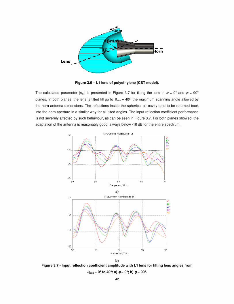
42

Figure 3.6 – L1 lens of polyethylene (CST model).

The calculated parameter |s11| is presented in Figure 3.7 for tilting the lens in ϕ = 0º and ϕ = 90º

planes. In both planes, the lens is tilted till up to θlens = 40º, the maximum scanning angle allowed by

the horn antenna dimensions. The reflections inside the spherical air cavity tend to be returned back

into the horn aperture in a similar way for all tilted angles. The input reflection coefficient performance

is not severely affected by such behaviour, as can be seen in Figure 3.7. For both planes showed, the

adaptation of the antenna is reasonably good, always below -10 dB for the entire spectrum.

a)

b)

Figure 3.7 - Input reflection coefficient amplitude with L1 lens for tilting lens angles from

θθθθlens = 0º to 40º: a) ϕϕϕϕ = 0º; b) ϕϕϕϕ = 90º.

θθθθt

Lens

Horn

5mm

8mm

43

The 3D far field radiation pattern for the non tilted lens case at f = 62.5 GHz is shown in Figure 3.8.

The correspondent directivity is 22.33 dBi with radiation efficiency above 96%.

Figure 3.8 – 3D radiation pattern for the non-tilted elliptical lens configuration.

In order to have a good perception of the steerable lens antenna performance for the entire scanning

space, being the lens tilted or rotated (meaning a beam rotation of 360º in azimuth and a beam tilt of

40º in relation to the feed axis), a beam tilt run was performed on both ϕ = 0º and ϕ = 90º planes of the

horn. Figure 3.9 presents the simulation results for both planes and although the feed radiation pattern

is different for both planes, the scanning behaviour is quite similar. Nevertheless, since the feed

presents different beam widths on both planes, the far field radiation pattern of the L1 lens follows that

same characteristic.

a)

44

b)

Figure 3.9 – Far field radiation pattern with L1 lens for tilting lens angles from

θθθθlens = 0º to 40º: a) ϕϕϕϕ = 0º; b) ϕϕϕϕ = 90º.

In order to confirm the broadband behaviour of the steerable lens, several simulations were run tilting

the lens on the ϕ = 0º plane for three frequencies: the central frequency f = 62.5 GHz and the two

other, at the Wireless HD spectrum edges, f = 57 GHz and f = 66 GHz. In Figure 3.10, for non tilted

lens, it is shown that for the lower frequency of the spectrum, in the ϕ = 0º plane, the far field radiation

pattern deviates slightly from the other frequencies performance, having a larger beam width and

higher side lobes, however, the difference is not very relevant.

a)

45

b)

Figure 3.10 – Far field radiation pattern with L1 lens covering the Wireless HD spectrum

(f = 57 GHz to f = 66 GHz): a) ϕϕϕϕ = 0º; b) ϕϕϕϕ = 90º.

When tilting the lens, Figure 3.11, the far field radiation pattern is identical for all frequencies,

validating the broadband lens premise, thus allowing the use of the entire Wireless HD frequency

band. The presented lens tilt angle corresponds to the maximum scanning angle, the worst possible

case.

Figure 3.11 – Far field radiation pattern with L1 lens for the Wireless HD spectrum

(f = 57 GHz to f = 66 GHz) for θθθθlens = 40º along the ϕϕϕϕ = 0º plane.

The undesired rays, which hit the surface outside the collimating region, contribute to the appearance

of an increasing left side lobe as the lens tilt increases. As will be seen ahead, this tends to pull the

maximum of the far field radiation pattern in the direction back to the feed axis, diminishing the lens

maximum scanning angle.

46

When comparing ILASH simulations with CST ones, one must take into account that ILASH

simulations just allow to consider reflections inside the lens with non tilted and on-axis feeds.

Considering this limitation, higher side lobe level is expected for CST simulations. On top of that,

elliptical lens presents a major difficulty when considering the GO/PO method, because geometrical

optics cannot cope with the rays spread when they reach the lens surface close to the critical angle of

incidence [34]. Figure 3.12 shows the incident angle at the outer lens surface accordingly with the

departing ray angle for the polyethylene elliptical lens.

Figure 3.12 – Incident angle at the outer lens surface in function of the departure angle from

the feed in relation to the lens axis.

At that point a surface wave is generated, originating a slightly more directive beam, while increasing

the side lobe level. It is seen in Figure 3.13 that the elliptical lens produces a lateral wave that results

from the fact that a high fraction of the horn’s radiation power is hitting the lens outer surface with an

incidence angle close to the interface critical angle, that corresponds to the total reflection condition

(presented angle corresponds to the polyethylene material):

� I �� = B () 7 �√��

9 = 40.7� (14)

Figure 3.13 – Near field for a lens tilt of θθθθlens = 20º.

0 20 40 60 80 1000

10

20

30

40

50

θ [º]

θi [º

]

θi

θc

θmax=49º

47

In Figure 3.13 it is possible to observe the surface wave travelling along the border of the lens and

mainly exiting the lens in the opposite direction. This effect is responsible for the high side lobe level

on the direction where the beam is tilted, representing a major disadvantage of the elliptical lens.

The obtained far-field radiation pattern for θlens = 0º at f = 62.5 GHz is presented in Figure 3.14. The

correspondent directivity is: CST, 22.33 dBi; ILASH, 22.26 dBi.

a) b)

Figure 3.14 – Radiation pattern for the non tilted L1 lens: a) ϕϕϕϕ = 0º; b) ϕϕϕϕ = 90º.

Simulations were performed with ILASH and CST software tools for different lens tilting angles along

the ϕ = 90º plane. Amplitude and phase results are presented, allowing a better comparison between

both software tools. Since reflections are not considered with ILASH, side lobe level and side lobe

phase are quite different from CST simulations, as it is shown from Figure 3.15 to Figure 3.18.

The radiation pattern for a lens tilt of θlens = 10º is presented in Figure 3.15. With CST the lens

radiation pattern presents a beam tilt of θbeam = 9º and a directivity of 22.09 dBi. With ILASH the beam

tilt is θbeam = 10º and the directivity is 22.08 dBi.

a) b)

Figure 3.15 – L1 lens radiation pattern for θθθθlens = 10º along ϕϕϕϕ = 90º: a) Amplitude; b) Phase.

48

The far field radiation pattern for the lens tilt of θlens = 20º is shown in Figure 3.16. The main beam tilt is

θbeam = 17.7º and the directivity is 21.16 dBi for CST, while for ILASH the beam tilt is θbeam = 19º and

the directivity is 21.52 dBi.

a) b)


Two more simulations were performed for a lens tilt of θlens = 30º and θlens = 40º. The corresponding

radiation patterns are presented in Figure 3.17 and Figure 3.18, respectively.

With CST, for θlens = 30º the maximum of radiation corresponds to θbeam = 26.3º while for θlens = 40º is

θbeam = 35.0º. The corresponding directivities are 20.37 dBi and 18.94 dBi, respectively. Using ILASH,

for θlens = 30º the radiation pattern tilt beam is θbeam = 28º and for θlens = 40º is θbeam = 37º. The

directivities are 20.43 dBi and 18.66 dBi.

The obtained radiation patterns for the five lens tilt positions have shown good agreement between

both software tools on the main beam; however, the beam tilt achieved with ILASH software tool does

not exactly corresponds to the one predicted with CST.

a) b)


49

a) b)


When just considering the ϕ = 90º plane, ILASH simulations predicted a more directive beam than

CST. However, ILASH simulations present higher side lobes for other planes, leading to a directivity

that closely follows the one obtained with CST.

By observing Table 3.1, one can see that Wireless HD standard requirement of 2 dB scanning loss

limit is only achieved till θbeam = 30º. This is due to the fact that the collimating region is only defined up

to θmax = 50º. The left side lobe is affected by the surface wave and the right side lobe by the radiation

power that is hitting the lens surface after the critical incidence angle, corresponding to the cylinder

shape, where the rays are no longer focused on the lens axis direction.

Table 3.1 – Performance parameters of L1 lens for ILASH and CST software tools.

Lens Tilt ILASH CST

θlens [º] θbeam [º] D [dBi] ∆D [dB] θbeam [º] D [dBi] ∆D [dB]

0º 0.0 22.27 0.0 0.0 22.33 0.0

10º 10.0 22.08 0.24 9.0 22.09 0.24

20º 19.0 21.52 0.75 17.7 21.16 1.17

30º 28.0 20.43 1.84 26.3 20.37 1.96

40º 37.0 18.66 3.61 35.0 18.94 3.39

As the lens tilt angle increases, the feed illumination gradually exceeds the defined maximum

scanning angle of the lens and so, part of the feed radiated power starts to build side lobes and

launches a surface wave along the lens outer interface, decreasing the beam directivity.

50

3.2. Solution with two refraction surfaces

The elliptical lens presents a reasonable performance for Wireless HD communication systems;

however, some limitations were shown. The difficulties encountered relied on the short collimating

area of the lens, not allowing a wide scanning angle. The objective of having a two refraction surfaces

lens is that a second degree of freedom will allow a maximization of the portion of the lens surface that

is able to collimate the feed’s radiation, increasing the lens θmax angle of incidence.

The two refraction surfaces lens formulation is based upon GO, with exiting rays from the outer

surface parallel to the lens axis. The lens geometry is presented in Figure 3.19.

T

F

2.35r

ε =

r(θ)

l(θ)

s(θ)

θ

γ(θ)

Figure 3.19 - Geometry for the design of two-refraction surface collimated beam lens

(extracted from [25]).

The inner surface, r (θ), is defined analytically using a Taylor series expansion in order to the angle

formed by the ray path departing from the feed (θ):

� �� = ∑ L�M�N: �� (15)

where Cc = F, C1 = 0 and C2...8 are the coefficients to optimize. C1 is null in order to impose ∂r/∂θ = 0 at

θ = 0º and so ensuring null refraction for the central ray. The outer shell can be defined by the angle

γ (θ) and the length of the rays l (θ). Using the Snell law condition at the inner shell interface leads to:

��

�� = √�� √�� (16)

By imposing an electrical path length condition we get:

� + √�� = � �� + √�� + �� (17)

with

�� = � + � − � ��"# �� − � ��"# �$ �� (18)

51

Since the inner shell profile is analytically defined by (15), the differential equation (16) can also be

determined analytically. F and T are input constants, defining the lens height, whereas r (θ) and γ (θ)

are unknown functions.

The optimization method consists on using the genetic algorithms (GA) formulation, where the C2…8

coefficients are generated as individuals on a larger population where a set of Cn parameters

corresponds to a unique solution of a lens. Setting the Cn coefficients defines the r (θ) function in (15)

so γ (θ) is calculated from (16) and then l (θ) is obtained from (17) and (18)(17). With r (θ), γ (θ) and l

(θ) the upper surface is defined. The above formulation is integrated on a GA optimization loop,

generating and testing different lens’ shapes, with the goal of maximizing θmax, as mentioned before.

Two constraints had to be added:

• r (θ) > 4.5 mm, to ensure that the horn edges never touch the lens surface when this is tilted;

• ray incidence angle at the upper lens interface must be below 95% of the critical angle.

The last constraint is included in order to minimize the excitation of a lateral wave along the lens upper

surface that tends to deflect part of the lens radiation away from the main beam direction reducing the

directivity. This occurs when ray’s incidence angles approach the total reflection condition (14).

The lens was designed with F = 5 mm and T = 20 mm to obtain a lens with similar size as the elliptical

one and identical directivity. The optimization process lead to:

� �� = 0.0274�M + 0.7683�Q + 0.4522�R + 0.2553�S + 0.3774�T + 0.7369�V + 0.7353�1 + 5 (19)

resulting in the lens profile presented in Figure 3.20.

a) b)

Figure 3.20 – L2 lens, ILASH model I: a) lens profile; b) lens surface.

52

Since the feed must be integrated into the lens when using ILASH configuration, a cylindrical air base

was added to the lens, down to 3 mm beneath the feed.

The maximum angle of collimation is for the present lens of 72º, Figure 3.21, wider than the 49º of the

elliptical lens. Since the lens does not surround the feed as it happened with the elliptical lens, it is

mechanically possible to tilt the lens for much wider angles.

Figure 3.21 – Ray tracing

3.2.1. L2 lens analysis with CST software

The L2 CST model is shown in Figure 3.22 and, comparing it with the L1 lens in Figure 3.6 is visible

that the L2 lens has a bigger radius than the L1 lens, although directivity is similar for both lenses. The

disadvantage of being a larger lens, since we are considering a movable lens, is fairly compensated

by the wider scanning angle accomplished by this lens.

Figure 3.22 – L2 CST model

θθθθmax=72º

53

When using a two refraction surface lens, a better behaviour is accomplished for the mechanical

scanning lens. The added constraint to avoid incidence angles close to the critical angle completely

eliminates the presence of a lateral wave. By comparing Figure 3.23 with Figure 3.12 it is visible that

the L2 lens incidence angles remain away from the critical angle for a wider scanning angle than the

L1 lens. In Figure 3.23 b) are represented the electromagnetic fields at a specific time, showing that in

opposition to the elliptical lens the lateral wave is not longer present, favouring a better beam steering

performance, with lower side lobes.

a)

b)

Figure 3.23 – a) Incident angle at the outer lens surface in function of the departure angle from

the feed in relation to the lens’ axis; b) near field for a lens tilt of θθθθbeam = 20º.

The parameter |s11| was calculated for six lens tilt angles, from θlens = 0º to θlens = 50º along the ϕ = 0º

and ϕ = 90º planes. For the non-tilted position of the lens, the reflections on the inner interface are

highly responsible for a weaker matching of the lens, as seen in Figure 3.24. By tilting the lens, the

matching improves significantly, since the reflections on the inner interface are deviated from the horn

aperture. For both ϕ = 0º and ϕ = 90º planes the input reflection coefficient is maintained under -10

dB, showing a fairly good matching of the antenna for the entire Wireless HD spectrum.

0 20 40 60 80 1000

10

20

30

40

50

θ [º]

θi [º

]

θi

θc

54

a)

b)

Figure 3.24 - Input reflection coefficient amplitude with L2 lens for tilting lens angles from

θθθθlens = 0º to 50º along: a) ϕϕϕϕ = 0º; b) ϕϕϕϕ = 90º.

The scanning performance of the lens is shown in Figure 3.25 when tilting it on planes ϕ = 0º and

ϕ = 90º. The lens presents a reasonably stable directivity (above 20 dBi) for the scanning angles

interval (from θlens = 0º to θlens = 50º), when tilting the beam on both mentioned planes of the horn. CST

simulations show a reasonable good result for a beam rotation of 360º in azimuth and a beam tilt of

θbeam = 50º in relation to the feed axis. The L2 lens shows a great improvement in relation to the L1

lens, having a lower scan loss and wider scanning angle amplitude. Exact performance values will be

presented ahead in Table 3.2.

55

a)

b)

Figure 3.25 – Far field radiation pattern with L2 lens for tilting lens angles from

θθθθlens = 0º to 50º along: a) ϕϕϕϕ = 0º; b) ϕϕϕϕ = 90º.

56

3.2.2. L2 lens analysis with ILASH software

Previous analyses of the L2 lens were run on the CST software tool. When evaluating the lens

antennas with CST, the structure dimensions in terms of wavelength are too big and so each

simulation becomes very time consuming. A faster software tool would be ILASH, although, as

showed before, the results are not as accurate as the CST ones when analyzing a lens antenna with

the feed outside the lens. However, in this case, since the lens is rotated accordingly with the feed

position, the spherical double shell lens at the lens base can be quite appropriate to overcome the

need of an integrated feed when using ILASH. The previously adapted solution in Figure 3.20,

consisted on having a cylindrical base, however, this approach is just valid on the interval θ = -72º to θ

= 72º, that corresponds to the original L2 lens. Instead of using a cylindrical base, a more suited shape

would be the spherical one, because for this case the wave coming from the feed that hits the lens

base suffers no deviation and for an outer shell with very low thickness the amplitude and phase

remains reasonably constant.

The spherical double shell lens consists on an inner air shell covered by a λ/10 thickness polystyrene

shell. The feed radiation direction suffers no relevant change; however, the amplitude is lowered due

to the interface reflection. The spherical lens is intended to simulate the absence of a lens interface,

which means that when evaluating its performance it is expected that the radiation pattern closely

approximates the one from the feed and that the radiation power is similar for both cases. As seen in

Figure 3.26 b), the radiation pattern suffers no significant change, while efficiency decreases to 94.5%.

The slight efficiency change is due to the outer interface, because even being a thin layer the reflected

power is large enough to influence a decay of 5.5% on the radiated power of the lens.

a) b)

Figure 3.26 – Spherical double shell lens: a) lens surface; b) radiation pattern compared to feed

radiation pattern (single mode feed)

57

The spherical lens is then added to the L2 lens, in a way that the lens profile is reasonably continuous

on the intersection point of the two lenses. The small differences described before will not influence

significantly the new lens model performance on ILASH when compared to the CST initial model.

To improve ILASH results accuracy the L2 lens shape was modified as stated before. The Figure 3.27

shows the ILASH model used. With this configuration, when tilting the lens in relation to the feed

position (with ILASH the feed is tilted instead), the lens base remains always spherical. Accordingly

with this and what was shown on the previous section the results obtained with ILASH for several lens

tilting positions are expected to closely approximate the CST ones.

One can see from the input reflection coefficient of the lens, shown in Figure 3.24, that for the non-

tilted case of the lens, the reflection on the inner interface represents an important factor that must be

consider when performing the ILASH L2 lens analysis. Although the outer shell of the spherical lens

has no significant interference on the overall performance of the lens, when considering internal

reflections, the reflected rays on the interface between the two shells will influence negatively the

radiation pattern on the opposite direction of those incident rays.

a) b)

Figure 3.27 – L2 lens, ILASH model with spherical base: a) lens profile; b) lens surface, inner

shell (blue) – air, outer shell (green) – polystyrene

The following two sections present simulated results of the modified L2 lens for non-tilted and tilted

positions of the lens (feed tilt when considering ILASH tool). The two cases are considered separately

because for the non-tilted case internal reflections can and must be taken into account when

evaluating the lens performance.

58

ILASH software tool, described in [35], was updated by the author in order to include the possibility of

tilting the feed. Considering the lack of time and the complexity of the kernel code associated with the

lens analysis, internal reflections can just be considered for the non-tilted feed case. In this way, just

for not-tilted cases is possible to consider the influence of internal reflections while evaluating the lens

performance. In Figure 3.28 the surface currents of the L2 lens are presented, considering no

reflections and 1st order reflections. At the top of the lens there are no significant differences, however,

the lens base is being more illuminated when reflections are included.

a) b)

Figure 3.28 – Surface currents - front view: a) no reflections; b) 1st

order reflections.

Figure 3.29 shows a better perspective of the lens base. The lens surface currents when considering

no reflections are presented in Figure 3.29a), distinctively showing the spherical lens base. With minor

differences, one can consider that the surface currents at the lens base approximately resemble the

feed far field radiation pattern, see Figure 2.22. When considering internal reflections, one can see

that there is a strong back radiation into the feed when taking reflections into consideration. Part of the

reflected rays should be obstructed by the horn antenna, but ILASH does not considerers the feed

presence. On the surrounding area of θ = 180º there is a maximum on the lens surface currents when

reflections are included, Figure 3.29 b) and c), demonstrating the behaviour it was expected from CST

simulations of the input reflection coefficient for the non-tilted position. On the horn ϕ = 0º plane, x-axis

plane, the lens base surface is illuminated on a slightly similar way for the three cases, but on the

other hand, in the ϕ = 90º plane the illumination with no reflections included is much weaker than for

the cases where reflections are considered, due to the feed radiation pattern asymmetric behaviour in

both planes. This relevant discrepancy will reflect on the far field radiation pattern as well, as will be

seen ahead. When considering internal reflections with this lens model, one must be very careful

when evaluating the results. Even with just 1st order reflections, the spherical lens base has a negative

impact on the lens radiation pattern; because the intended ‘neutral’ effect of the sphere is just

achieved for the rays departing from the feed (the sphere centre) and therefore, any reflected ray

returning from the lens surface is erroneously changed by the spherical lens base.

59

a)

b) c)

Figure 3.29 – Surface currents - base view: a) no reflections; b) 1st

order reflections;

c) 2nd

order reflections

After the considerations made earlier, it is important to notice that the far field radiation patterns

obtained with ILASH correspond to a variation of the CST lens model and so, both applications cannot

be compared on base of these results in terms of accuracy. The lens models are different and what

was intended was to obtain an ILASH lens model that fairly approximates the lens behaviour when the

feed is placed outside the lens.

The far field radiation pattern of the lens (ILASH simulation) is shown in Figure 3.30, superimposed on

the previous CST simulation for both ϕ = 0º and ϕ = 90º planes. The lens simulations in ILASH

consisted on a first step by neglecting internal reflections and in a second one by including 1st order

reflections. When comparing to the CST results, for ϕ = 90º, Figure 3.30 b), a big improvement on the

side lobe level is achieved by including internal reflections. The low side lobe level of the far field

radiation pattern when neglecting internal reflections is due to the fact that the reflected rays on the

inner interface are not considered on the surface currents and therefore on the radiation pattern. For

ϕ = 0º is not so heavily affected by the internal reflections because, as seen in Figure 2.22, the far field

radiation pattern of the feed presents a much higher side lobe level on that plane that for ϕ = 90º.

60

a)

b)

Figure 3.30 - Radiation pattern for the non-tilted feed (lens) configuration with 1st

order

reflections: a) ϕϕϕϕ = 0º; b) ϕϕϕϕ = 90º.

The inclusion of 2nd order reflections presents a problem for this specific lens model, since the

reflected rays on the spherical base, which should have no interference in the rays’ trajectory, are

going to hit the lens surface on the opposite direction of the rays’ incidence. Figure 3.31 shows the

comparison between simulations without reflections and with 2nd order reflections. Although the far

field radiation pattern presents a similar side lobe level for both CST and ILASH simulations, a

stronger ripple on the secondary lobes in ILASH analysis indicates that the spherical lens base is

erroneously adding reflected rays with relative high power to the lens surface currents, negatively

influencing the radiation pattern.

61

a)

b)

Figure 3.31 - Radiation pattern for the non-tilted feed (lens) configuration with 2nd

order


When observing the phase of the radiation pattern of the lens, Figure 3.32 and Figure 3.33, it is

perfectly visible that ILASH and CST simulations agree quite well till θ approximately equal to 70º, the

maximum angle of incidence of the original lens. The radiation pattern phase confirms what was

stated before, showing a more unstable phase behaviour when 2nd order reflections are considered.

The present study, considering the influence of internal reflections on the accuracy of the lens analysis

also demonstrates that the directivity of the lens output is slightly affected by the reflections at the

inner interface, which are due to the relative large difference of permittivity between the environment

(air) and the lens material (polyethylene). Considering no reflections the radiation pattern directivity is

23dBi, while for 1st and 2nd order reflections the directivity is 22.6dBi and 21.9dBi, respectively.

62

a)

b)

Figure 3.32 - Radiation pattern phase for the non-tilted feed (lens) configuration with 1st

order


a)

63

b)

Figure 3.33 - Radiation pattern phase for the non-tilted feed (lens) configuration with 2nd

order


With ILASH, when using a tilted feed, the internal reflections are not considered for the lens surface

currents calculations. In the direction of the feed main beam it presents a reasonable accuracy, being

the effect of reflections negligible. The feed is tilted in the ϕ = 90º plane, in order to compare with the

lens tilt on CST. Figure 3.34 shows that the spherical double shell lens is strongly illuminated when the

feed is tilted near θfeed = 40º or above. Tilting the feed radiation pattern leads to a new relative

maximum on the base of the lens, corresponding to the feed main beam amplitude, Figure 3.34 b).

a) b)

Figure 3.34 – Surface currents – tilted feed on the ϕϕϕϕ = 90º plane: a) θθθθfeed = 10º; b) θθθθfeed = 40º.

The far field radiation pattern is collimated on the direction of the lens axis, what in the case of tilting

just the feed leads to have the radiation pattern main beam at the origin position. In order to compare

these results with the CST ones, the ILASH far field radiation patterns are shifted by the

corresponding lens tilt angle θlens.

64

Tilting the feed leads to a big portion of feed radiated power to pass outside the lens, being this energy

accounted by using the spherical double shell lens. This solution showed to be relatively accurate as

seen before and if internal reflections could be used for tilted feeds, the ILASH simulation results

would probably be more precise. By observing Figure 3.35 to Figure 3.39 one can see that ILASH

simulations are in good agreement with the CST ones in amplitude and in phase as well, when

considering just the main lobe and the right side lobe. The not so good agreement on the left side is

due to the not accounted internal reflections when tilting the feed to the right. On the direction of the

feed main beam the phase is accurately calculated, being the discrepancies found where the feed

radiation pattern amplitude is below -30 dB, when the power associated with internal reflections is of

the same order or even higher. By tilting the lens or the feed a second lobe grows accordingly with the

tilted angle, corresponding to an increase of power that is avoiding the lens surface along the

propagation path. Although the right and left side lobes have similar amplitude, as mentioned before,

the left lobe is due to reflections on the lens inner interface.

a b)

Figure 3.35 – Radiation pattern for the θθθθlens = -10º lens configuration along the ϕϕϕϕ = 90º plane:

a) Amplitude; b) Phase.

a) b)



65

a) b)



a) b)



a) b)



66

In Table 3.2 is presented the performance parameters of the L2 lens for ILASH (without reflections)

and CST software tools. By observing the results it is seen that both tools present close predictions of

the lens behaviour. The directivity is higher with ILASH because the power from the reflected rays is

not considered on the lens surface currents calculation, which results on a low side lobe level of the

far field radiation pattern. With ILASH a less accurate result is determined when compared to CST

simulations, however, as a first prediction of the lens behaviour and since it just takes a few minutes to

analyse it, ILASH tool can be considered a helpful and powerful tool, enabling to obtain several

performance indicators of the lens in a very short time. Each simulation of the studied lens on CST

takes about 1 to 2.5 hours to compute on the same pc as the ILASH takes 6 minutes.

Table 3.2 – Performance parameters of L2 lens for ILASH and CST software tools.

Lens Tilt ILASH CST

θlens [º] θbeam [º] D [dBi] ∆D [dB] θbeam [º] D [dBi] ∆D [dB]

0 0.0 23 0 0.0 21.5 0.31

10 9.68 22.81 0.19 8.7 21.69 0.12

20 19.2 22.45 0.55 18.2 21.81 0.0

30 28.72 21.89 1.11 26.9 21.4 0.41

40 38 21.12 1.88 36.5 20.61 1.2

50 47 20.04 2.96 45.5 19.65 2.16

The directivity variation (using CST tool) is reasonably small inside the tilting interval of θ = -50º to

θ = 50º, around 2 dB, inside the scan loss allowed on the Wireless HD requirements. Gain is showed

in Figure 3.40 for the entire spectrum of the Wireless HD communication system (from f = 57 GHz to

f = 66 GHz). With a close to 1 dB gain variation over the entire bandwidth it is shown that L2 lens is a

reasonably good scanning and broadband lens, especially tailored for the Wireless HD standard.

Figure 3.40 - Gain variation of the L2 lens versus tilt angle computed for three frequencies

within the Wireless HD band.

67

4. Mm-wave antennas measurements

This chapter presents all relevant information of the shaped dielectric lenses’ tests. Concerning the

manufacturing process, the adopted lens fabrication technique for this case, a single material lens,

corresponds to the machining technique using a CNC milling machine. All procedures are fully

described in [30]. Being a single shell lens with the feed not integrated at the lens base, its fabrication

process is quite simple and it represents a low-cost solution if molding technique is used. The two

main sections ahead include a description of the measurement facilities and further analysis of the

lenses’ prototypes measurements.

4.1. Measurement facility description

Antenna radiation pattern measurements are performed in a 4.1 m × 2.4 m × 2.1 m millimetre wave

anechoic chamber, Figure 4.1. The measurement process, data acquisition, manipulation and

visualization are controlled by a software application, [36], developed by former IST students and now

updated by the author. Azimuth rotation of the antenna under test was driven by an ORBIT AL-360

positioner, while antenna roll axis and probe polarization were manually controlled. As part of the

project, it was necessary to modify the software tool in order to remotely control all the measurements

procedures, incrementing the laboratory measuring capabilities.

Figure 4.1 – Mm-wave anechoic chamber.

The software application that controls the anechoic chamber measurements was updated in terms of

making it more user-friendly and especially to enable it to remotely control the antenna roll axis and

probe polarization using ORBIT AL-060 positioners. The automation of lens and probe rotation

represents a higher step when considering measurements accuracy. It also allows running several

measurements without user interference, decreasing possible user error and releasing him from

repetitive tasks.

68

In Figure 4.2 a) are presented all available devices. Three devices were added to the previous list: the

Agilent PNA Series Network Analyzer and the two ORBIT AL-060 positioners. The PNA Series

Network Analyzer from Agilent is used as a frequency synthesizer device and as a field measuring

device. It enables measuring the radiation pattern amplitude and phase and is especially used for

polarization measuring. The two ORBIT AL-060 positioners, together with the AL-360 positioner

already installed, are responsible for allowing a complete automation of the antennas measurements.

The software application allows the user to attribute any desired rotation axis to each positioner, see

Figure 4.2 b), among the three presented: antenna azimuth, antenna polarization and probe

polarization. In this way, no manual intervention is needed from the user when measuring the antenna

radiation pattern for several antenna and probe positions.

a) b)

Figure 4.2 – Devices: a) Initialization; b) Selection.

The user-friendly interface is now more intuitive and easier to use. Along with the minor changes

introduced, to correct small errors or to improve the application performance, the application flow chart

was strongly modified. Four main sections were created taking advantage of the past software

structure: Radiation, Polarization, Post-processing and Devices. Among those, just the

Post-processing interface stays unchanged; however, this interface is now available at any time,

enabling the user to view and manipulate old curves without having to perform any measuring or even

to initialize any device. In the previous version, stages were sequential and a certain order of events

69

had to be followed. As seen in Figure 4.2 a), each device must be initialized prior to use. The

procedure of initialization is now slightly different, giving the user total control over all available

devices. At any time the devices can be changed, reinitialized with different parameters and even

selected for other functions when considering the axis measuring devices.

The field measuring window for azimuth rotation of the lens is shown in Figure 4.3. Taking advantage

of the introduced PNA Series Network Analyzer, both amplitude and phase can be measured. It is also

important to mention that with this device the frequency used can go till f = 110 GHz. The polarization

window includes a new functionality, which allows one to perform a frequency sweep for specific

antenna and probe orientations, taking advantage of the former routines used for polarization

measurements.

Figure 4.3 – Field measuring window.

Although the software has been updated with all the mentioned fixtures and particularly with the two

ORBIT AL-060 positioners, the anechoic chamber just has the ORBIT AL-360 fully functional. The

installation of both positioners is waiting for a free time window of measurements, after which the

anechoic chamber measurements will be entirely remotely controlled.

70

4.2. Antennas’ prototypes and measurements

This section includes all manufactured prototypes and respective measurements. The designed

lenses are intended to work on a Wireless HD communication system or a similar service. As shown in

Figure 4.4, the lens must pivots over the horn in a way that the radiation beam is tilted accordingly with

the lens movement. The lens can perform an elevation and an azimuth scanning, depending on the

lens axis rotation. By properly rotating and tilting the lens, the radiation beam is collimated on a

specific direction, since the rays that exit the outer lens interface are always parallel to the lens axis.

The manufactured lens geometries were described in section 3. Measurements will confirm that the

lenses performance closely fulfil the Wireless HD requirements.

a) b)

Figure 4.4 – Geometry of the horn plus lens antenna: a) non-tilted lens; b) tilted lens

(based on [14]).

For test purposes, a prototype of the mechanical scanning lens concept was designed, being the lens

tilt manually controlled. Out of the project scope is the antenna automatic rotation mechanism, which

is currently being studied in a parallel project. A drawing of the lens concept is presented in Figure 4.5,

where the stationary horn is placed in a way it radiates to the movable lens. The lens tilting axis,

passes along the horn phase centre, and this axis is defined by pivots in the two lens extensions that

support the lens. The structure formed by the lens and the arms can rotate azimuthally around the

horn, making it possible to test the lens performance over the entire 360º azimuth scanning space.

The geometry adopted, together with the lens characteristics make this antenna a low-cost and

efficient solution for slower tracking situations, like Wireless HD or HAPs services. The presented

mechanical scanning lens structure and concept are the subject of the patents requests [14] and [37],

pending for approval.

71

Figure 4.5 – Structure of the mechanical scanning lens (taken from [14]).

The horn antenna that feeds the movable lens, previously described in 2.2.2, was manufactured in

aluminium with 7.8 mm inner aperture diameter, 10 mm flared length and 3.9 mm diameter circular

waveguide port, Figure 4.6.

Figure 4.6 – Manufactured circular horn feed.

The horn is fed in the TE11 mode with right-hand circular polarization. The measured radiation pattern

of the standalone circular horn at f = 62.5 GHz is represented in Figure 4.7, superimposed on the CST

simulations. A general good agreement is shown between measurements and simulations, both for

co- and cross-polarization. When comparing the lens performance indicators obtained by measuring

and simulation, a strong similarity is found. The measured gain is 13.6 dBi, close to the 13.7 dBi gain

predicted by CST and the input reflection coefficient |s11| is always below -20 dB for both simulated

and measured cases, as shown in Figure 4.8. The discrepancy between simulations and

measurements is due to the inclusion of the polarization device at the feed that slightly influences the

reflection coefficient.

72

Figure 4.7 - Measured and simulated co- and cross-polar radiation pattern of the standalone

conical horn at 62.5 GHz.

Figure 4.8 - Measured amplitude input reflection coefficient of the horn antenna superimposed

on CST simulations.

As mentioned before, the selected material for lenses fabrication was polyethylene. The permittivity

and loss tangent values were measured at f = 62.5 GHz using the Fabry Perot open resonator

method. Description of the method is found at [30]. Two lenses were manufactured: the elliptical dome

lens and the solution with two refraction surfaces, respectively L1 and L2.

4.2.1. Steerable elliptical dome lens

The manufactured lens weights just 5 g, making it easy to tilt and rotate. The manufactured

mechanical scanning lens prototype is shown in Figure 4.9, with the L1 lens included. With this lens no

additional lens’ extensions were needed, since the lens rotation axis is inside the spherical cavity. A

compass was added at the lab test set-up for easy reading of the manually adjusted lens tilt angles.

73

Figure 4.9 - Manufactured L1 lens and feeding horn, assembled in a lab test set-up.

The measured input reflection coefficient |s11| at the horn port is shown in Figure 4.10 for the entire

Wireless HD spectrum. Different tilt angles were tested and the results were superimposed on the

standalone horn measurements. The lens spherical cavity reflects part of the radiation into the horn,

as |s11| parameter increases with the inclusion of the lens. Although there is a |s11| increase for the

entire bandwidth of Wireless HD, it remains always below an acceptable -10 dB level, as predicted

with CST, Figure 3.7. The lens performance is very similar for different tilt angles, explained by the

spherical shape of the inner cavity.

Figure 4.10 – Measured amplitude input reflection coefficient of the horn antenna when placed

in the centre of the spherical air cavity of the L1 lens.

The lens far field radiation pattern were measured for different tilt angles in the interval θlens = 0º to

θlens = 40º (the lens maximum scanning angle) with f = 62.5 GHZ. In Figure 4.11 are shown the co-

and cross-polarization results, presenting a gain of 21.6 dBi for the non-tilted position of the lens and

gradually decreasing for higher lens tilts. The radiation beam is also heavily deformed when increasing

the lens tilt. The cross-polarization level in the main beam direction is always below -15 dB for all lens

tilts measured, indicating that the lens preserves the circular polarization of the circular horn and that

the reflected wave at the spherical cavity does not interfere much with the horn’s radiation pattern and

polarization.

74

The measured results are superimposed on the CST simulations and the agreement between them is

remarkable, both for co- and cross-polarization.

Figure 4.11 - Measured and simulated radiation patterns of the L1 lens antenna at f =62.5 GHz

for θθθθlens = 0º to θθθθlens = -40º along ϕϕϕϕ = 90º.

To summarize the lens behaviour, lens performance indicators were obtained from the measured

results for different tilt angles and presented in Table 4.1. The main beam direction (θbeam), presents

an increasing difference in relation to the lens tilt angle (θlens), diminishing the maximum scanning

angle to near ±25º if considering a 2 dB scan loss gain as the limit, with radiation efficiency always

above 96%.

Table 4.1 - Measured performance of the L1 lens at f = 62.5 GHz. ∆∆∆∆G is the gain scan loss, XPol

is the higher cross polarization level in the main beam full width at -10 dB and ηηηη is the CST

simulated radiation efficiency.

L1 Lens

θlens [º] θbeam [º] G [dBi] ∆G [dB] XPol [dB] η (%)

0 0.0 21.6 0.2 -18.5 96.1

10 8.9 21.8 0.0 -18.5 96.6

20 17.3 20.9 0.9 -17.6 96.7

30 25.6 19.7 2.1 -16.4 97.0

40 32.5 19.1 2.7 -14.9 97.5

75

4.2.2. Solution with two refraction surfaces

The second lens, called L2, was manufactured and placed at the lab test set-up the same way as L1,

Figure 4.12. It weights 8 g, slightly larger than the previous one. In this case the lens tilting axis lies

outside the lens volume, so two lateral extensions of the same material had to be added to provide

fixing points for lens tilting. The presence of these extensions hardly affects the lens radiation pattern

because they are not illuminated by the horn main lobe.

Figure 4.12 - Manufactured L2 lens plus horn feed.

The measured return loss |s11| at the circular horn input port is shown in Figure 4.13. For non-tilted

position, the lens behaviour is similar to the elliptical dome lens, with |s11| slightly below -10 dB,

however, by increasing the lens tilt the input reflection coefficient |s11| decreases significantly. Since

the inner interface is no longer spherical and is more close to a flat surface, the slight reflected wave

at the bottom of the lens is deflected away from the horn aperture.

Figure 4.13 – Measured amplitude input reflection coefficient of the horn antenna when placed

in the centre of the spherical air cavity of the L1 lens.

76

The measured radiation pattern of the L2 lens, for f = 62.5 GHz, is shown in Figure 4.14. Both co- and

cross-polarization radiation patterns are presented for tilt angles from θlens = 0º to θlens = 50º, with steps

of 10º. The improvement from the elliptical lens is quite remarkable. The L2 lens presents

considerable lower scanning loss gain than the L1 lens and also presents a much better defined main

beam up to the maximum scan angle of 45º. The marginal beam deformation with tilt angle is not

critical for the Wireless HD application. The measured results are superimposed on the CST prediction

and the agreement is excellent for both co- and cross-polarization.

Figure 4.14 - Measured and simulated radiation patterns of the L2 lens antenna at f =62.5 GHz

for θθθθlens = 0º to θθθθlens = 50º.

The CST accuracy proven against measurements validates the simulation model and the previous

showed analysis for other frequencies in the Wireless HD band.

The performance indicator values of the L2 lens, obtained through measurements, are presented in

Table 4.2. The measured gain is very stable along all tilted angles, with 21.7 dBi for the non-tilted

position. The maximum beam steering angle corresponds to θbeam = 45º, with just a 1.1 dB of beam

steering loss, much better than the L1 lens. As to radiation efficiency and cross-polarization the

performance is similar to the L1 one, with efficiency above 95% and a considerably low cross-

polarization always below -16 dB for all lens tilt angles.

The Wireless HD standard defines the lens elevation beam steering till ±40º, being fully achieved by

the presented antenna, however, considering the 2 dB margin established, a wider beam tilt can be

accomplished beyond the θbeam = ±45º.

77

Table 4.2 - Measured performance indicator values of the L2 lens at f = 62.5 GHz. ∆∆∆∆G is the scan

loss value, XPol is the higher cross polarization level in the main beam full width at -10 dB and

ηηηη is the CST simulated radiation efficiency.

L2 Lens

θlens [º] θbeam [º] G [dBi] ∆G [dB] XPol [dB] η (%)

0 0.0 21.7 0.0 -17.3 95.3

10 9.7 21.7 0.0 -16.2 95.5

20 19.5 21.7 0.0 -16.5 95.4

30 27.9 21.7 0.0 -16.5 95.8

40 36.4 21.2 0.5 -16.4 96.0

50 44.8 20.6 1.1 -16.5 97.0

The results showed for this particular lens, demonstrate the antenna remarkable performance when

considering its scanning attributes. The mechanical beam steering lens fulfils with all the Wireless HD

requirements, making it a viable and adequate solution for such communication service. The

mechanical steerable lens prototype showed very good results, close to what was expected from CST

simulations, proving the mechanical beam steerable antenna concept.

79

5. Conclusions

A new steerable beam antenna concept was developed and proved against Wireless HD

requirements, being the same design principles valid for different applications, such as the HAPs

system. The presented solution, making use of a collimating lens, corresponds to a totally new

scanning concept, although collimating lenses are widely used for scanning purposes. The beam

steering is obtained by pivoting an appropriately shaped dielectric lens in front of a single fixed feed,

instead of the regular matrix of feeds located at a fixed lens. The proposed mechanical beam steering

antenna is simple, compact and it represents a low-cost solution for large scale production.

When considering the optimization of a double refraction surfaces lens, the lens performance greatly

improves when comparing it to an elliptical lens, mainly due to the extra degree of freedom. The

fabricated mechanical steerable lens prototype fully complies with the Wireless HD requirements,

demonstrating a ±45º elevation scan capability over full azimuth with gain scan loss lower than 1.1 dB

and radiation efficiency above 95% for the entire spectrum of the referred standard (from f = 57 GHz

to f = 66 GHz). The lens weights only 8 g, which for mechanical steering is a critical quality.

In order to adjust the presented lens antenna to a different application, namely the HAPs, the new lens

would be designed for HAPs system in the Urban Area Coverage, with a scanning angle of

θbeam = ±60º. The polyethylene lens was specifically designed for the Wireless HD standard, but higher

beam tilt angles can be achieved by using materials with higher permittivity. For the change in the

operating frequency and associated gain a scaling of the complete solution would almost be enough to

comply with the HAPs requirements.

Complete antenna analysis were performed with CST, however, a full performance comparison was

made with ILASH tool, since lens antenna simulations are much faster when using ILASH. Its

performance and accuracy were already massively tested and studied when considering integrated

feeds at the lens base; however, for the particular case where the feed is placed outside the lens,

some adjustments had to be considered. By changing the lens profile accordingly with specific rules,

the overall results closely approach the CST ones. ILASH proved to be a relative accurate and reliable

software tool for lens design and as a first lens performance indicator.

The software application that is required for the measurement process, data acquisition, manipulation

and visualization used with the millimetre wave anechoic chamber was improved in terms of its

structure and organization, making it more flexible and easier to use. Its user-friendly interface

suffered some changes; however, the most important additions were the two ORBIT AL-060

positioners and the PNA Series Network Analyzer from Agilent. The inclusion of the positioners made

the antenna and probe rotation a completely remote control system, enhancing the laboratory

capabilities. On the other hand, the PNA Series Network Analyzer allows performing antenna analysis

over a wider range of frequencies, till f = 110 GHz.

81

6. References

[1] Jong-Hoon Lee; Kidera, N.; Pinel, S.; Laskar, J.; Tentzeris, M. M.; “60 GHz High-Gain

Aperture-Coupled Microstrip Antennas using Soft-Surface and Stacked Cavity on LTCC

multilayer technology”, IEEE Antennas and Propagation Society International Symposium, pp.

1621–1624, July 2006.

[2] Hiroki Tanaka and Takashi Ohira, “Beam-Steerable Planar Array Antennas Using Varactor

Diodes for 60-GHz-Band Applications”, European Microwave Conf., Munich, 2003.

[3] Abbas Abbaspour-Tamijani, Kamal Sarabandi, “An Affordable Millimeter-Wave Beam-

Steerable Antenna Using Interleaved Planar Subarrays”, IEEE Trans. on Antennas and

Propagation, vol. 51, no. 9, Sept. 2003.

[4] A. Tombak and A. Mortazawi, “A Novel Low-Cost Beam-Steering Technique Based on the

Extended-Resonance Power-Dividing Method”, IEEE Trans. Microwave Theory Tech., vol. 52,

no. 2, pp. 664-669, Feb. 2004.

[5] K. Van Caekenberghe, T. Vaha-Heikkila, G. Rebeiz and K. Sarabandi, “Ka-Band MEMS TTD

passive electronically scanned array (ESA)”, IEEE Antennas and Propagation Society

International Symposium, pp. 513-516, July 2006.

[6] Kai Chang, Ming-yi Li, Tae-Yeoul Yun, Christopher T. Rodenbeck, “Novel Low-Cost Beam-

Steering Techniques”, IEEE Trans. on Antennas and Propagation, vol. 50, no. 5, May 2002.

[7] Donald H. Kuhn, “Dual Lens Antenna with Mechanical and Electrical Beam Scanning”, United

States Patent, US 4.642.651, Feb. 1987.

[8] Archer David Munger, “Scanning Array Antenna using Rotating Plates and Method of

Operation Therefor”, United States Patent, US 5.945.946, Aug. 1999.

[9] Zimmerman, K. A.; Wann, J. E.; Freeman, R. A.; Black, D. N.; Marsik, J. C.; “Scanning

Directional Antenna with Lens and Reflector Assembly”, United States Patent, US 6.396.448,

May 2002.

[10] Gary M. Hamman, Douglas W. Taylor, “Surveillance Radar Scanning Antenna Requiring no

Rotary Joint”, United States Patent, US 6.556.174 B1, Apr. 2003.

[11] Dean Alan Paschen, Kiersten Carinne Kerby, “Low-Profile Lens Method and Apparatus for

Mechanical Steering of Aperture Antennas”, United States Patent Application Publication, US

2007/0285327 A1, Dec. 2007.

[12] http://www.wirelesshd.org “WirelessHD Specification Version 1.0 Overview”, Oct. 2007.

[13] Robert C. Daniels and Robert W. Heath, Jr., “60 GHz Wireless Communications: Emerging

Requirements and Design Recommendations”, IEEE Vehicular Technology Magazine, pp. 41-

50, Sept. 2007.

82

[14] J. Costa, C. Fernandes, E. Lima, “Antena compacta com orientação mecânica do feixe de

radiação, para seguimento de terminais móveis em comunicações sem fios”, Portuguese

Patent, PT 104108, Patent pending, Jun. 2008.

[15] Stylianos Karapantazis and Fotini-Niovi Pavlidou, “The Role of High Altitude Platforms in

Beyond 3G Networks”, IEEE Wireless Communications, pp. 33-41, Dec. 2005.

[16] J. Thornton, D. Grace, C. Spillard, T. Konefal and T. C. Tozer, “Broadband Communications

from a High-Altitude Platform: the European Helinet Programme”, Electronics &

Communication Engineering Journal, June 2001.

[17] Zain Elabdin Omer Elshaikh, Md. Rafiqul Islam, Ahmad Faris Ismail and Othman O. Khalifa,

“High Altitude Platform for Wireless Communications and Other Services”, Intern. Conf. on

Electrical and Computer Engineering, ICECE 2006, Dhaka, Bangladesh, pp. 432-438, Dec.

2006.

[18] Recommendation ITU-R F.1500, “Preferred Characteristics of Systems in the Fixed Service

Using High Altitude Platforms Operating in the Bands 47.2-47.5 GHz and 47.9-48.2 GHz”,

2000.

[19] Kandus, G.; Svigelj, A.; Mohorcic, M.; “Telecommunication Network Over High Altitude

Platforms”, Intern. Conf. on Telecommunications in Modern Satellite, Cable and Broadcasting

Services, vol. 2, pp. 344-347, Sept. 2005.

[20] Pawlowski, W., “Radio Wave Propagation Effects in High-Altitude Platforms Systems”, Intern.

Conf. on Microwaves, Radar and Wireless Communications, MIKON-2000, vol. 1, pp. 185-

188, May 2000.

[21] Bon-Jun Ku, Yang-Su Kim, Byung-Su Kang, Do-Seob Ahn, A. S. Belyaev, Ye. N. Egorov, N.

V. Vladimirov, S. A. Ganin, A. C. Reutov, Yu. A. Suserov, A. M. Shitikov, A. V. Shislov, A. G.

Shubov, “Multi-Faced and Multibeam DBF Antenna for High Altitude Platform Station Stages

of Antenna Development”, Intern. Conf. on Antenna Theory and Techniques, Sevastopol,

Ukraine, pp. 87-90, Sept. 2003.

[22] Recommendation ITU-R F.1843, “Methodology for Determining the Power Level for High

Altitude Platform Stations Ground Terminals to Facilitate Sharing with Space Station

Receivers in the Bands 47.2-47.5 GHz and 47.9-48.2 GHz”, 2007.

[23] E. Lima, J. Costa, M. Silveirinha, and C. Fernandes, “ILASH – Software Tool for the Design of

Integrated Lens Antennas”, Proc. IEEE APS/URSI Symposium, San Diego, CA, USA, July

2008.

[24] Jorge R. Costa, Carlos A. Fernandes, Eduardo B. Lima, Mário Silveirinha, Marten van der

Vorst, “Design of an Integrated Lens Feed for an Imaging Reflector System using the ILASH

Software Tool”, Proc. ESA Workshop on Antennas for Earth Observation, Science,

83

Telecommunication and Navigation Space Missions, Noordwijk, Netherlands, vol.1, pp. 378–

381, May 2008.

[25] Jorge R. Costa, Eduardo B. Lima, Carlos A. Fernandes, “Compact Beam-Steerable Lens

Antenna for 60 GHz Wireless Communications”, IEEE Trans. on Antennas and Propagation

Special Issue on Antennas and Propagation Aspects of 60 – 90 GHz Wireless

Communications, 2008.

[26] Eduardo B. Lima, Jorge R. Costa, Carlos A. Fernandes, “Mechanical Beam-Steerable Elliptical

Dome Lens”, European Conference on Antennas and Propagation, Berlin, Germany, March

2009 (pending for evaluation).

[27] M. Born, E. Wolf, “Principles of Optics”, N. York, Pergamon, 1959.

[28] A. Peebles, “A Dielectric Bifocal Lens for Multibeam Antenna Applications”, IEEE Trans.

Antennas and Propagation, Vol. 36, no. 5, pp. 599-606, May 1988.

[29] Jorge R. Costa, Mário G. Silveirinha, Carlos A. Fernandes, Eduardo B. Lima, “Shaped Double-

Shell Integrated Lens Antenna for Imaging Applications”, Internal Report, IT/RMOM/ILASH/IR,

Instituto de Telecomunicações, May 2006.

[30] Carlos A. Fernandes, Jorge Costa, Mário Silveirinha, “Final Report of ILASH Project”,

IT/RMOM/ILASH/FR/01/v1, July 2007.

[31] http://www.cst.com.

[32] D. Filipovic, S. Gearhart and G. Rebize, “Double-Slot Antennas on Extended Hemispherical

and Elliptical Silicon Dielectric Lenses”, IEEE Trans. Microwave Theory Tech., vol. 41, no. 10,

pp. 1738-1740, Oct. 1993.

[33] J. Costa, C. Fernandes, G. Godi, R. Sauleau, L. Le Coq and H. Legay, “Compact Ka-band

Lens Antennas for LEO Satellites”, IEEE Trans. Antennas and Propagation, vol. 56, no. 6, pp.

1251-1268, May 2008.

[34] D. Pasqualini, S. Maci, “High-Frequency Analysis of Integrated Dielectric Lens Antennas”,

IEEE Trans. Antennas and Propagation, vol. 52, pp. 840-847, March 2004.

[35] Eduardo Lima, João Henriques, Carlos A. Fernandes, Jorge R. Costa, Deliverable 3 – ILASH

User’s Manual – final version, IT/RMOM/ILASH/D/02/v3, 30-July-2007.

[36] Andreia Fernandes, João Cunha, “Control Software for Anechoic Chamber Antenna

Measurements”, Licenciatura, Sept. 2003.

84

[37] J. Costa, C. Fernandes, E. Lima, “Antena compacta com orientação mecânica do feixe de

radiação, para seguimento de terminais móveis em comunicações sem fios”, Portuguese

Design Patent, Patent pending, Jun 2008.

A-1

A. Annexes

A.1. Prototype structure

The antenna is formed by a shaped dielectric lens and by a supporting structure, which allows the lens

to rotate and tilt. A stationary horn antenna is placed beneath the lens in order to illuminate it with an

electromagnetic wave. The lens is axial symmetric and two lateral extensions are attached to it,

enabling the lens to tilt in relation to a horizontal axis, defined by the horn aperture. As can be seen in

Figure A.1, the lens is supported by two vertical arms that are attached to the structure base. The

entire body previously described can be rotated around the symmetry axis of the fixed horn antenna.

In this way, the lens axis can aim at any direction inside a conical region, centred at the horn axis.

Figure A.1 – Prototype structure.

A-2

A.2. Manufactured Prototypes' Photos

Figure A.2 – Solution with two refraction surfaces (L2 lens)

A-3

Figure A.3 – Steerable elliptical dome lens (L1 lens)

A-4

a) b)

Figure A.4 – Horn antenna photos: a) front view; b) top view.

a) b)

Figure A.5 – Mechanical Beam Steering structure, without the feed attached:

a) side view; b) front view.

Mechanical Steerable Lens for Wireless Communications · uma lente dieléctrica oscila sobre uma...

Documents

Transcript of Mechanical Steerable Lens for Wireless Communications · uma lente dieléctrica oscila sobre uma...