Mechanical microcontacts of powder particles studied...
129
Mechanical microcontacts of powder particles studied with the quartz crystal microbalance Dissertation zur Erlangung des Grades „Doktor der Naturwissenschaften“ Am Fachbereich Chemie, Pharmazie und Geowissenschaften der Johannes Gutenberg-Universität Mainz Ewa Maria Vittorias geboren in Poznan, Polen Mainz, November 2010
Transcript of Mechanical microcontacts of powder particles studied...

Mechanical microcontacts of powder particles studied with the quartz
crystal microbalance
Dissertation
zur Erlangung des Grades
„Doktor der Naturwissenschaften“
Am Fachbereich Chemie, Pharmazie und Geowissenschaften
der Johannes Gutenberg-Universität Mainz
Ewa Maria Vittorias
geboren in Poznan, Polen
Mainz, November 2010

Dekan:
Erstgutachter:
Zweitgutachter:
Tag der mündlichen Prüfung: 26. Januar 2011

Die vorliegende Arbeit wurde am Institut für Physikalische Chemie der
Johannes-Gutenberg Universität Mainz
und am Max-Planck-Institut für Polymerforschung in Mainz unter der
Betreuung von
in der Zeit von Mai 2006 bis Juli 2009 angefertigt.

Things are in motion part of the time and again they are at rest; They are in motion when Love tends to make one out of many,
Or Strife tends to make many out of one, And in the intervening time they are at rest.
Empedokles


Abstract
Within this work, a particle-polymer surface system is studied with respect to the
particle-surface interactions. The latter are governed by micromechanics and are an important
aspect for a wide range of industrial applications. Here, a new methodology is developed for
understanding the adhesion process and measure the relevant forces, based on the quartz
crystal microbalance, QCM.
The potential of the QCM technique for studying particle-surface interactions and
reflect the adhesion process is evaluated by carrying out experiments with a custom-made
setup, consisting of the QCM with a 160 nm thick film of polystyrene (PS) spin-coated onto
the quartz and of glass particles, of different diameters (5-20µm), deposited onto the polymer
surface. Shifts in the QCM resonance frequency are monitored as a function of the oscillation
amplitude. The induced frequency shifts of the 3rd overtone are found to decrease or increase,
depending on the particle-surface coupling type and the applied oscillation (frequency and
amplitude). For strong coupling the 3rd harmonic decreased, corresponding to an “added
mass” on the quartz surface. However, positive frequency shifts are observed in some cases
and are attributed to weak-coupling between particle and surface. Higher overtones, i.e. the 5th
and 7th, were utilized in order to derive additional information about the interactions taking
place. For small particles, the shift for specific overtones can increase after annealing, while
for large particle diameters annealing causes a negative frequency shift. The lower overtones
correspond to a generally strong-coupling regime with mainly negative frequency shifts
observed, while the 7th appears to be sensitive to the contact break-down and the recorded
shifts are positive.
During oscillation, the motion of the particles and the induced frequency shift of the
QCM are governed by a balance between inertial forces and contact forces. The adherence of
the particles can be increased by annealing the PS film at 150°C, which led to the formation
of a PS meniscus. For the interpretation, the Hertz, Johnson-Kendall-Roberts, Derjaguin-
Müller-Toporov and the Mindlin theory of partial slip are considered. The Mindlin approach
is utilized to describe partial slip. When partial slip takes place induced by an oscillating load,
a part of the contact ruptures. This results in a decrease of the effective contact stiffness.
Additionally, there are long-term memory effects due to the consolidation which along with
the QCM vibrations induce a coupling increase. However, the latter can also break the
contact, lead to detachment and even surface damage and deformation due to inertia. For
strong coupling the particles appear to move with the vibrations and simply act as added

effective mass leading to a decrease of the resonance frequency, in agreement with the
Sauerbrey equation that is commonly used to calculate the added mass on a QCM). When the
system enters the weak-coupling regime the particles are not able to follow the fast movement
of the QCM surface. Hence, they effectively act as adding a “spring” with an additional
coupling constant and increase the resonance frequency. The frequency shift, however, is not
a unique function of the coupling constant. Furthermore, the critical oscillation amplitude is
determined, above which particle detach. No movement is detected at much lower amplitudes,
while for intermediate values, lateral particle displacement is observed.
In order to validate the QCM results and study the particle effects on the surface, atomic
force microscopy, AFM, is additionally utilized, to image surfaces and measure surface
forces. By studying the surface of the polymer film after excitation and particle removal,
AFM imaging helped in detecting three different meniscus types for the contact area: the “full
contact”, the “asymmetrical” and a third one including a “homocentric smaller meniscus”.
The different meniscus forms result in varying bond intensity between particles and polymer
film, which could explain the deviation between number of particles per surface area
measured by imaging and the values provided by the QCM - frequency shift analysis. The
asymmetric and the homocentric contact types are suggested to be responsible for the positive
frequency shifts observed for all three measured overtones, i.e. for the weak-coupling regime,
while the “full contact” type resulted in a negative frequency shift, by effectively contributing
to the mass increase of the quartz..
The interplay between inertia and contact forces for the particle-surface system leads to
strong- or weak-coupling, with the particle affecting in three mentioned ways the polymer
surface. This is manifested in the frequency shifts of the QCM system harmonics which are
used to differentiate between the two interaction types and reflect the overall state of adhesion
for particles of different size.

1
Contents
1. Introduction....................................................................................................................... 3
2. The Quartz Crystal Microbalance..................................................................................... 7
2.1 Quartz crystal resonator ............................................................................................. 7
2.1.1 Vibrational modes and orientation angle ........................................................... 8
2.1.2 Effective properties of the quartz crystal resonator ......................................... 10
2.1.3 Impedance analysis .......................................................................................... 12
2.1.4 Lateral amplitude distribution and energy trapping ......................................... 13
2.1.5 Equation predicting the amplitude of motion of quartz crystal resonators ...... 14
2.1.6 The Butterworth-van-Dyke (BvD) electrical equivalent circuit ...................... 16
2.2 Quartz crystal microbalance..................................................................................... 20
2.2.1 Sauerbrey equation – deposited mass calculation ............................................ 21
2.2.2 Adsorption on the quartz crystal resonators..................................................... 22
2.2.3 Physical interpretation of the Sauerbrey thickness .......................................... 23
3. Mechanical contact between bodies ............................................................................... 25
3.1 Surface forces........................................................................................................... 25
3.2 Surface forces measurements techniques................................................................. 28
3.2.1 Atomic Force Microscopy................................................................................ 29
3.2.2 Centrifuge technique ........................................................................................ 32
3.3 Van der Waals interactions between particles and surfaces..................................... 33
3.4 Contact models......................................................................................................... 37
3.5 Particle – surface coupling ....................................................................................... 43
3.5.1 Strong- and weak-coupling limit...................................................................... 46
3.5.2 Extension of the Dybwad model to many spheres ........................................... 50
3.5.3 Distribution of contact stiffness ....................................................................... 55
3.5.4 Amplitude dependence of frequency and bandwidth....................................... 57
3.5.5 Lateral stiffness of multi-asperity contacts ...................................................... 64

2
4. Materials and methods .................................................................................................... 66
4.1 Experimental setup................................................................................................... 66
4.2 Materials and sample preparation ............................................................................ 69
5. Results and discussion .................................................................................................... 73
5.1 QCM oscillation amplitude ...................................................................................... 73
5.2 Critical amplitude for particle detachment............................................................... 74
5.3 Contact between particles and polymer-film ........................................................... 78
5.3.1 Reproducibility issues ...................................................................................... 87
5.4 Effect of overtone order ........................................................................................... 88
5.4.1 Amplitude sweeps ............................................................................................ 89
5.4.2 Particles – surface interaction .......................................................................... 91
5.5 Calculation of particles per surface area .................................................................. 96
6. Atomic Force Microscopy – Force Measurements and Surface Imaging ...................... 98
6.1 Force measurements – colloidal probe technique .................................................... 98
6.2 Adhesion force measurements ............................................................................... 100
6.3 Surface changes caused by particles - Surface Imaging ........................................ 102
6.3.1 Surface quality................................................................................................ 102
6.3.2 Surface damage by the particles..................................................................... 103
6.3.3 Meniscus formation........................................................................................ 106
7. Summary and conclusions ............................................................................................ 115
References .............................................................................................................................. 118
Acknowledgements ................................................................................................................ 122
3
1. Introduction
The ancient Greek found that they needed only two fundamental forces to account for
all natural phenomena. One was Love, the other was Hate. The first brought things together
while the second caused them to part. The idea was first proposed by Empedocles around 450
B.C. and after it was “improved” by Aristotle, it formed the basis of chemical theory for
nearly 2000 years 1.
The fundamental forces of nature are nowadays accepted to be separated in 4 types. Two
of these are strong and weak interactions that act between neutrons, protons, electrons and
other elementary particles. These two forces have a very short range of action, typically less
than 10-5 nm, and are relevant for the fields of nuclear and high-energy physics. The other two
fundamental forces arise from the electromagnetic and gravitational interactions. These act
between atoms and molecules, as well as between elementary particles. The gravitational and
electromagnetic forces, such as the Coulomb interactions, are effective over a much larger
range of distances, from subatomic to practically infinite distances, e.g. gravitational
attraction between planetary objects. The above types are consequently the forces that govern
the behaviour of everyday things. Thus, their accurate detection, measurement, modelling and
possibly control is a main goal of modern physics (as well as classical physics in the past
centuries). One manifestation of attractive forces is in the adhesion between two materials.
Adhesion can be understood as an attraction between two solid bodies with a common contact
surface that has been produced by the existence of intermolecular attractive forces that are
active at short distances 2.
Adhesion between powders and surfaces plays an important role in several technological
areas and processes, such as paste drying operations, fluidization of fine particles,
microencapsulation, xerography and imprinting. Furthermore, it is a crucial process in the
food and pharmaceutical industry with limitless and important applications. In this important
technological field control of adhesion can enhance operation efficiency and reduce the
production cost in the industrial processes 3.
Due to the above mentioned importance the adhesion force holds in several processes, it
has become necessary to carry out more detailed studies aiming at determining the magnitude
of adhesion forces between a plane surface and particles. This study and understanding is
extended to different formats, sizes and chemical structure of particles and surfaces. For this
research field, a methodology was already developed as early as the 17th century. This early

4
interest on these phenomena demonstrates their importance and explains their later industrial
relevance. The first experimental technique was based on the centrifugal technique described
initially by Polke 4,5 and later by Booth and Newton 6 and Lam and Newton 7-9, which was
used to investigate particle size influence on the particle-surface adhesion force.
Within this work the surface – particle interactions are studied with a different approach.
More specifically the interactions are described and quantified using micromechanical
theories. Micromechanical contacts are important from the fundamental point of view and in
many applications. As mentioned above, the mechanical interaction between fine particles
determines the flow of granular materials. It is relevant for the cleaning of surfaces, for
example in the semiconductor industry and the dispersion of powders to aerosols, which is
crucial e.g. in asthma treatment. Another application is in lubrication of microcontacts which
make commercial application of microelectromechanical systems (MEMS) devices with
sliding surfaces very challenging 10. As a further example, “acousto-lubrication” is being
investigated as a potential mechanism to promote dry lubrication of MEMS devices by
manipulating the micromechanical contacts 11-13.
In a general manner, understanding of friction and adhesion between solid bodies has to
be based on the knowledge of the exact shape of their mechanical contact, which usually
consists of microcontacts. Therefore, the quantification and modelling of microcontacts have
been studied extensively 14,15. Although the importance is easily acknowledged and despite
the extensive investigation performed in the past, a fundamental understanding is lacking, due
to at least two reasons.
Firstly, experiments in which the adhesion force is determined, as a microcontact
property, show wide distributions rather than a single value. Adhesion forces vary by
typically a factor of two to ten even within relatively monodisperse powders 16-20. Even when
measuring the adhesion force between smooth silicon oxide particles taken from one batch,
adhesion forces may differ by a factor two from one pair of particles to the next 21. As a cause
of this variation surface roughness and surface heterogeneity had to be taken into account22-27.
Roughness can change significantly in the contact area between two particles, depending on
the precise location of the contact. Heterogeneity in chemical composition or molecular
structure at different length scales can cause a different energy of adhesion. Thus, it can cause
a variation in the effective adhesion force depending on the precise location of contact.
Second, direct measurements of adhesion forces, or rolling and sliding friction of
particles are technically demanding, expensive, and of limited applicability. This includes
experiments with the centrifuge technique 28 and the atomic force microscope (AFM) 29, the
5
two most widely used techniques. Though both techniques have provided us with valuable
insights, they also have their limits. With the centrifuge contact times are in the order of hours
and after detachment no further experiments can be carried out with the same particle. In the
case of AFM experiments, each individual particle has to be attached to the end of a
microcantilever. The contact direction is predetermined and not free to adjust. Both
techniques are not applicable for routine applications and are experimentally demanding.
Therefore, a simple alternative technique is desired, that can have a potential application in
the industry, where fast, robust and accurate force testing is required.
A promising method for this application could be the quartz crystal microbalance,
QCM. Usually the QCM is applied to measure the mass per unit area of homogeneous thin
films. The measurement principle is based in the fact that the resonance frequency of the
quartz decreases if the added mass is increased. However, for contacts between a QCM and
particles with a size in the micron range, the frequency is found to increase 30. The frequency
increase is closely related to the stiffness of the contact and may therefore be used to probe
this stiffness. Furthermore QCM testing is relatively fast, less challenging experimentally as
the above mentioned methods. Finally, the method has unique applications due to the fact that
one is able to probe mechanical material behaviour at high frequency excitations, as high as
MHz range.
Within this work, experiments with glass particles of variable size on a QCM system are
described. The aim is to evaluate the potential of QCM as a method for determining the nature
and measuring the strength of microcontacts between surfaces and particles. Therefore, the
influence of surface adhesion and inertia of the particles on the response of a QCM is
analysed. Surface effects are found to be more important for small particles, while for the
large particles inertia should dominate their movement and interaction. For this reason experi-
ments are carried out with particles of different diameters, small and large (but all in the µm
range). When the particles are attached to the QCM-film surface, the resonance frequency of
the quartz crystal is changed. The latter is monitored for different excitation amplitudes.
Several phenomena are observed, such as the so-called partial slip, which leads to a decrease
of the resonance frequency with increasing amplitude in some (but not all) cases. The
resonance frequency is correlated to particle adhesion force, vibration and generally
interaction of the particles with the polymer film.
Any macroscopic movement of the particles was imaged with video microscopy which
was coupled to the QCM setup in order to provide with a direct monitoring of the process

6
taking place during the excitation of the system. The particles were deposited onto thin films
of polystyrene (PS) which had been spin-coated onto the QCM surface. After analysing the
physisorbed particles, the sample was annealed at temperatures above the glass-transition
temperature, Tg, of the polymer. The changes on the film surface caused by the particle
movement and excitation, e.g. meniscus formation, are observed, analysed and interpreted.
The thesis is divided into seven main parts:
In the second chapter, the quartz crystal microbalance is introduced and the main
properties of this tool are described. The main focus is in the application of QCM for
adhesion force measurements and the suggested technique is demonstrated.
In chapter three, the theory of surface forces with the focus on adhesion force is
presented. It includes also a description of the main methods that have been used for adhesion
investigation. These were mainly the atomic force microscopy method, AFM, and the
centrifuge technique. The non-modified, or classical, AFM set-up is described in more detail.
In the fourth chapter, the used materials, as well as the experimental set-up design are
exhibited. Furthermore the sample preparation is described in detail.
Chapter five presents the results obtained by QCM in detail and interpretations are put
in relations with the introduced models and with the theory.
In chapter six, the study of the surface before and after the excitation is described. The
changes caused by particles during the quartz oscillation were depicted by surface imaging
with AFM. Furthermore, the adhesion force is alternatively measured by colloidal probe
technique and the results are presented.
In chapter seven, the main results of the thesis, using the experimental technique and
setup as presented, are summarized. The work ends with the provided conclusions on the
applicability of QCM for studying micromechanical contacts.

7
2. The Quartz Crystal Microbalance
Quartz is one of several forms of silicone dioxide (SiO2) that is found as a crystalline
form in nature. High purity natural quartz is costly to mine. Consequently, most of the quartz
used for crystal fabrication today is of the ‘cultured’ or synthetic variety. Cultured quartz is
produced by placing small seeds of quartz mixed with an alkaline solution in an autoclave.
This mixture is subjected to high heat, typically above 4000 C and high pressure,
approximately 30,000 psi. This causes the quartz to dissolve and reform as thin slices. This
process takes approximately 30-45 days 31,32. Quartz crystal has a density of 2649 kg/m3 and a
melting temperature of 1750oC. It is ideal for use as a frequency determining device, due to its
predictable thermal, mechanical, and electrical characteristics. The quartz crystal resonator is
one of the few devices that can provide a high quality factor, Q, i.e. a high ratio of stored to
dissipated energy, that is needed for precise frequency control tools 32.
2.1 Quartz crystal resonator
The quartz crystal resonator consists of a thin plate of a piezoelectric material that can
be electrically excited to oscillate in a thickness shear mode. The piezoelectric effect was
found by the Curies in 1880. The word piezoelectricity literally means “pressure electricity”.
The prefix piezo- is derived from the Greek word πιεζό = to press. Generally speaking, a
material is called piezoelectric if mechanical deformation leads to an electrical polarization
(piezoeffect). The piezoelectric effect of quartz describes the appearance of electric charge on
the surface of a crystal due to mechanical periodic deformation. Inversely, application of an
electric voltage provokes a mechanical deformation. Thus, an alternating voltage leads to a
periodic alternating deformation, i.e. an oscillation of the piezoelectric crystal 32.
The quartz crystal resonator operates due to the inverse piezoelectric effect, which is
only found in crystals without any center of inversion. Crystals with an inversion center do
not show piezo-electricity but are also mechanically deformable by application of an electrical
field. This effect is called electro-striction and is several orders of magnitude weaker than
piezoelectricity 32.

8
2.1.1 Vibrational modes and orientation angle
The QCM crystal surface undergoes a tangential shear motion. There are many different
vibrational shear modes for crystals as shown in Fig. 2.1.
Thickness Extensional
Fundamental
3rd Overtone
5th Overtone
Face Shear Length-WidthFlexure
Thickness Extensional
Fundamental
3rd Overtone
5th Overtone
Face Shear Length-WidthFlexure
Fig. 2.1: Vibrational modes for quartz crystal.
One characteristic factor of the quartz crystal is the resonance frequency as a function of
temperature. This property is primarily determined by the orientation angle at which the
quartz wafers are cut from a given bar of quartz. These properties are dependent on the
reference directions within the crystal. These directions are referred to as ‘axes’. There are
three axes in quartz, the X, the Y, and the Z. An ideal crystal would consist of a hexagonal
prism with six facets at each end. A cross section taken from that prism would look like the
depiction in Fig. 2.2. The Z-axis is known as the optical axis and the crystal repeats its
physical properties every 1200 as it is rotated about the Z-axis. The X-axis is parallel to a line
bisecting the angles between adjacent prism faces. This axis is called the electrical axis.
Electrical polarization occurs in this direction when mechanical pressure is applied. An XT-
cut crystal is produced from a slab of quartz cut from that portion of the quartz bar that is
perpendicular to the X-axis. The Y-axis, which is also known as the mechanical axis, runs at

9
right angles though the face of the prism and at right angles to the X-axis. Most Y-axis crystals
vibrate in their ‘sheer modes’; face shear for low frequency CT- and DT-cut crystal, and the
thickness shear for higher frequency AT- and BT-cut crystals.
The AT-cut is the most popular of the Y-axis group because of its excellent frequency
vs. temperature characteristics, i.e. its properties-stability under a broad temperature range
(zero-temperature coefficient). The AT-cut is produced by cutting the quartz bar at an angle of
approximately 35o15’ from the Z-axis. Ideally, an AT-cut quartz oscillates exhibiting a pure
shear motion of the surface. The surface move parallel with respect to each other and the
thickness of the plate does not change, i.e. there is no normal component of motion.
R
m
r
x
s
r
AT
mm
Z’
x’ y’
R
m
r
x
s
r
AT
mm
Z’
x’ y’
Fig. 2.2: An idealized left-handed quartz crystal showing the 35.150-inclined AT-cut plane (adapted from Bottom 32). R-faces are called major, r the minor rhomb faces. The s and x are very rare, but when occurring enable one
to distinguish between right and left quartz.

10
2.1.2 Effective properties of the quartz crystal resonator
The QCM crystal resonator is usually a circular disc. The thickness, hq of the disc of the
shear resonator is related to the fundamental mode frequency, f0 by the following equation:
q
AT
q
qqto h
Nh
Gcf ===
2
/ ρ
λ Eq. 1
where λ is the wave length of the oscillation and ct is the transversal velocity of sound. An
explanation of the variables and respective values is given in the Table 2.1. Knowing the
thickness hq of the quartz plate the resonance frequency can easily be calculated using the
frequency constant, NAT. The even harmonics usually cannot be excited because the shear
induced polarisation averages to zero. The excitation is however possible for the odd
multiples of the excitation frequency:
0fnf n ×≈ Eq. 2
where n = 1, 3, 5, …
density (ρq) 2649 kg/m3
eff. shear modulus (Gq) 2.957·1010 N/m3
eff. piezoelectric constant (e’26) 9.65·10-2 C/m2
eff. dielectric constant (εq) 40.3·10-12 F/m
piezoelectric coefficient (d’26 = e’26/Gq) 3.21·10-12 m/V
piezoelectrical coupling constant (κ2) 0.0080
frequency constant (NAT) 1660 kHz mm
acoustic impedance (Zq) 8.77·106 kg/m2s
Table 2.1: Effective physical properties of AT-cut crystalline quartz. Adapted from Bottom 32.

11
Because the frequency of the crystal is related to its thickness, there is a limitation in the
manufacturing of high frequency fundamental crystals. The higher the frequency that is
applied, the thinner the crystal blank should be.
The so-called Q-factor of a crystal is the quality factor of the motional parameters at
resonance. The maximum frequency stability of a crystal is directly related to its Q-factor.
The higher the Q factor is, the smaller the bandwidth appears and the steeper the reactance
curve is. In order to provide stability of the resonance frequency, a high quality-factor and a
minimized electromechanical coupling are needed. The quality-factor, Q is defined as:
cycleperdissipatedenergycycleperstoredenergyQ___
___2π= Eq. 3
The quality-factor of the shear mode oscillation in atmospheric air and room temperature of
an AT-cut quartz is approximately Q = 105. The electromechanical coupling-factor K is
determined by the resulting piezo-coefficient eq = 9.65·10-2 C/m2, the actual dielectric constant
054.4 ∈⋅=∈q , where 120 10854.8 −⋅=∈ C/(Vm) is the dielectric constant, and the shear modulus
µq = 2.93 · 1010 N/m2
091.0__
__≈==
qeenergyelectricalstored
energyelasticstoredKεµ
Eq. 4

12
2.1.3 Impedance analysis
The measurements performed within this work, to study particle-surface contacts by
quartz crystal resonator are based on impedance analysis. This is the methodology of using
the conductance curve of the crystal. The conductance as a function of frequency is measured,
therefore providing a means to electrically determine the acoustic resonance. The central
parameters of measurements are the resonance frequency f, and the half-maximum-half-
width, Γ. In resonance, both the amplitude of motion and the electrical conductance show a
maximum. When the frequency of excitation matches the acoustic resonance frequency, the
amplitude of oscillation becomes large. Simultaneously, the current through the electrodes, as
well as the conductance, increases. Because the current is large on resonance, the resonance
can be easily found with purely electrical instrumentation. Measuring the conductance around
the resonance frequency, one obtains a resonance curve. The experimental results are fitted to
a theoretical resonance curve, the Lorentz curve. The resonance frequency and the bandwidth
are extracted from the fit 33,34. A typical curve obtained by single measurement is presented in
the Fig 2.3. The frequency shift is proportional to the area-averaged stress-speed ratio at the
crystal surface, however complex the sample may be.
Fig. 2.3: Typical curve obtained by impedance analysis, fitted to a theoretical resonance curve – Lorentz curve
(blue).
fit
13
The impedance analysis, as described above, has significant advantages in the analysis
of QCM experiments. Both the frequency and the bandwidth are obtained by a single
measurement simultaneously. The additional parameters, such as the amplitude of the
resonance, which is related to the effective area of the plate, and the offset of the susceptance,
which is the imaginary part of admittance (inverse of impedance) with conductance being the
real part. Both amplitude and susceptance, which is related to the dielectric environment of
the resonator, are measured as well. However, the accuracy for the determination of the last
two parameters is lower than the one obtained for the frequency measurement. Finally,
impedance analysis offers the ability to measure a large number of higher harmonics, as high
as e.g. 25 in air atmosphere or as high as 10 in liquid medium. Thereby the wavelength of
shear sound can be varied.
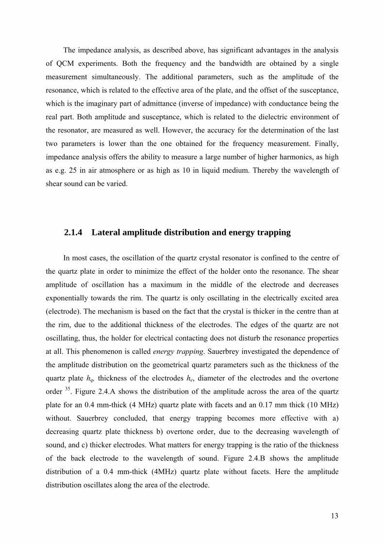
2.1.4 Lateral amplitude distribution and energy trapping
In most cases, the oscillation of the quartz crystal resonator is confined to the centre of
the quartz plate in order to minimize the effect of the holder onto the resonance. The shear
amplitude of oscillation has a maximum in the middle of the electrode and decreases
exponentially towards the rim. The quartz is only oscillating in the electrically excited area
(electrode). The mechanism is based on the fact that the crystal is thicker in the centre than at
the rim, due to the additional thickness of the electrodes. The edges of the quartz are not
oscillating, thus, the holder for electrical contacting does not disturb the resonance properties
at all. This phenomenon is called energy trapping. Sauerbrey investigated the dependence of
the amplitude distribution on the geometrical quartz parameters such as the thickness of the
quartz plate hq, thickness of the electrodes he, diameter of the electrodes and the overtone
order 35. Figure 2.4.A shows the distribution of the amplitude across the area of the quartz
plate for an 0.4 mm-thick (4 MHz) quartz plate with facets and an 0.17 mm thick (10 MHz)
without. Sauerbrey concluded, that energy trapping becomes more effective with a)
decreasing quartz plate thickness b) overtone order, due to the decreasing wavelength of
sound, and c) thicker electrodes. What matters for energy trapping is the ratio of the thickness
of the back electrode to the wavelength of sound. Figure 2.4.B shows the amplitude
distribution of a 0.4 mm-thick (4MHz) quartz plate without facets. Here the amplitude
distribution oscillates along the area of the electrode.

14
Fig. 2.4: Amplitude distribution along quartz plates (adapted from Sauerbrey 35).
2.1.5 Equation predicting the amplitude of motion of quartz crystal
resonators
The amplitude of motion is of substantial interest for experiments probing interfacial
mechanical behaviour. Using the transmission line model published in 1948 by Mason,
Johannsmann and Heim 36 have provided the simple equation, which predicts the amplitude of
motion of quartz crystal resonators, uo. They calculate the amplitude, u0, from the speed as:
0,26220,26
22,26
0014144
211
elelqq
oelqqf
QUdn
QUcZ
en
QUde
Znnfuu
ππππω====
•
Eq. 5
where ff is the frequency of the fundamental, n is the overtone order, Q is the quality factor, •
u is the lateral speed of motion. The parameter 1226 101.3 −×=d V/m is the piezoelectric strain
coefficient. The driving voltage Uel,0 is often quoted in terms of the electrical power in units
of decibel, where 0 dBm corresponds to a power of 1mW (see Chapter 4.1).

15
When the dBm values are used, the equation is simplified to the form of:
Vpm
nd
nQUa
el22622
125.114==
π Eq. 6
During this work the applied amplitude of the quartz oscillation was calculated using the
above equation.
Concerning the energy trapping and amplitude distribution it can be assumed the mass-
sensitive area is situated in the central part of the resonator, covering about the area where the
two electrodes overlap. Distribution of the mass sensitivity closely follows the vibration
amplitude distribution. Both the mass sensitivity and amplitude distribution curves follow a
Gaussian function 37.
Following Johannsmann 36, the effective area, A, of the quartz crystal resonator can be
calculated from the Q- factor and the motional resistance R1
2226
max
32 fq fdZn
QG
A π= Eq. 7
where 0,
0,max
el
el
UI
G = is the peak conductance (Iel,0 – electric current, Uel,0 – voltage), and is one
of the fit parameters in impedance analysis, it is the inverse of the motional resistance R1. The
factor sm
kgZ q 28.8= is the acoustic impedance of AT-cut quartz, and ff is the fundamental
resonance frequency. The larger the effective area is the more current is drawn at the peak of
the resonance. The back electrode confines the amplitude to the centre of the crystal via
energy trapping.
16
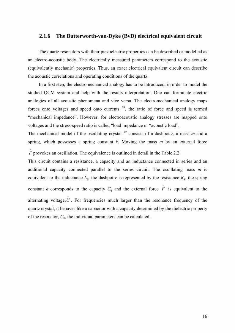
2.1.6 The Butterworth-van-Dyke (BvD) electrical equivalent circuit
The quartz resonators with their piezoelectric properties can be described or modelled as
an electro-acoustic body. The electrically measured parameters correspond to the acoustic
(equivalently mechanic) properties. Thus, an exact electrical equivalent circuit can describe
the acoustic correlations and operating conditions of the quartz.
In a first step, the electromechanical analogy has to be introduced, in order to model the
studied QCM system and help with the results interpretation. One can formulate electric
analogies of all acoustic phenomena and vice versa. The electromechanical analogy maps
forces onto voltages and speed onto currents 38, the ratio of force and speed is termed
“mechanical impedance”. However, for electroacoustic analogy stresses are mapped onto
voltages and the stress-speed ratio is called “load impedance or “acoustic load”.
The mechanical model of the oscillating crystal 39 consists of a dashpot r, a mass m and a
spring, which possesses a spring constant k. Moving the mass m by an external force ~F provokes an oscillation. The equivalence is outlined in detail in the Table 2.2.
This circuit contains a resistance, a capacity and an inductance connected in series and an
additional capacity connected parallel to the series circuit. The oscillating mass m is
equivalent to the inductance Lq, the dashpot r is represented by the resistance Rq, the spring
constant k corresponds to the capacity Cq and the external force ~F is equivalent to the
alternating voltage,~
U . For frequencies much larger than the resonance frequency of the
quartz crystal, it behaves like a capacitor with a capacity determined by the dielectric property
of the resonator, C0, the individual parameters can be calculated.

17
Mechanical Electrical
Force = Area · Stress F = A ·σ Voltage U
Speed •
u Current I
Mechanical Impedance •• ==u
Au
FZ mσ Electrical Impedance
IUZel =
Mass mp pm miu
FZ ω== • Inductance L LiZel ω=
Dash pot with
Drag coefficient ξ ξ=mZ Resistance R RZel =
Spring with
Spring constant κ ωκ
ω iuiF
u
FZ m === •
Capacitance C Ci
Zel ω1
=
Table 2.2: Electromechanical equivalence.
The quartz crystal can be represented electrically by the circuit shown in Fig. 2.5. The
motional inductance (Lm), motional capacitance (Cm), motional resistance R1 and a parallel
capacitance C0 and series resistance in all there motional parameters can be measured using a
crystal impedance (CI) meter 40.
(iωC0)-1
(iωC1)-1
iωL1 R1
Acoustic branch
Electrical branch
M D W
v(t)F(t)
R
L
C
U(t)
I(t)
(iωC0)-1
(iωC1)-1
iωL1 R1
Acoustic branch
Electrical branch
(iωC0)-1
(iωC1)-1
iωL1 R1
Acoustic branch
Electrical branch
M D W
v(t)F(t)
M D W
v(t)F(t)
R
L
C
U(t)
I(t)
R
L
C
U(t)
I(t)
Fig. 2.5: Butterworth-van Dyke equivalent circuit for a quartz crystal resonator and electro-mechanical analogy
(adopted from Berg 41). Acoustic is the part of the system which resonates in the specific frequency range and
electric is the branch where the mechanical is transformed to electrical energy.

18
Below shown are the fundamental equations used to describe the circuit.
motional inductance: 226
3
8Aeh
L qqm
ρ= Eq. 8
motional resistance: δπ tan8 2
26
2
nZAed
R qq
m = Eq. 9
motional capacitance: qq
m AGndAe
C 2
226
)(8π
= Eq. 10
parallel capacitance: qh
AC 0
0εε
= Eq. 11
with ρq the density, hq the thickness of the plate, A the effective area, 226 1065.9 −×=e C/m2 a
piezoelectric coefficient, Zq the acoustic impedance, tan(δ) = Gq”/Gq’ the loss tangent, n the
overtone order, Gq the storage modulus, ε the dielectric constant of quartz, and ε0 the
dielectric permittivity of vacuum. The meaning of the parallel capacitance can be readily
explained and consists of the electrical capacitance across the electrodes. The parameters Lm,
Rm, and Cm are not strictly electrical quantities, but rather describe the mechanical response of
the system.
With regard to the graphical representation of mechanical elements there is a subtlety: when
two mechanical elements are placed in series, their elongations add up, while the force
transmitted through the elements is constant. On the contrary, when two electrical elements
are placed in series, the voltages are additive and the current is constant.
The piezo-effect is graphically represented as a transformer in Fig. 2.5. The transformer
turns mechanical quantities into electrical ones according to a parameter termed φ2 , which
can be calculated by:
qhAe26=φ Eq. 12
Using the above given parameter, the lateral speed at the crystal surface can be calculated as:
mIuφ21
=•
Eq. 13
19
The resulting stress is equivalently:
mUφσ 2= Eq. 14
and the mechanical impedance is given by the following relation:
mmech ZZ 24φ= Eq. 15
here, •
u is the lateral speed at the crystal surface, σ is the stress, •
= uAZ mech /σ is the
mechanical impedance, A is the active area (which is similar but not identical to the area of
the back electrode and may vary with overtone order), 226 1065.9 −×=e C/m2 the piezoelectric
stress coefficient, and hq the thickness of quartz plate.
The BvD equivalent circuit possesses two resonance frequencies due to the parallel
configuration, the antiresonance fA, corresponding to the whole circuit, and the series
resonance fs, corresponding to the upper serial branch and the quartz resonance frequency
(noted as acoustic branch in Fig. 2.5) 42. The two resonance frequencies can be calculated by
Kirchoff’s laws:
⎟⎟⎠
⎞⎜⎜⎝
⎛+=
0
11121
CCLf
qqA π
Eq. 16
qqs CL
f 121π
= Eq. 17

20
2.2 Quartz crystal microbalance
Quartz crystal is used for a wide range of applications and responds to many other
experimental parameters and conditions, such as temperature, applied stress, and viscosity of
the surrounding medium. The capability of microweighing gave the quartz crystal
microbalance its name. The quartz crystal microbalance technique has been used to measure
mass of the deposited thin films for over 50 years. This method for mass measurements was
introduced in 1959 by Sauerbrey 43 and became a largely used instrument for small mass
measurements in vacuum, gas and liquid phase 38,41,44. The use of QCM as a mass change
detector is the most widely known. The new challenge is to combine the quartz crystal
resonator with other techniques such as surface plasmon resonance spectroscopy (SPR),
surface forces apparatus 45, atomic force microscopy (AFM), and others 34.
Usually the quartz crystal microbalance, QCM, is applied to measure the mass per unit
area of homogeneous, rigidly attached thin films, and the analysis of microweight
experiments is based on the Sauerbrey equation. During this study quartz crystal
microbalance was used as a tool for contact mechanics experiments, based on the Sauerbrey
model.
Furthermore, the QCM method can be used as a tool to determine viscoelastic properties
of the films adjacent to the quartz surface from the combined evaluation of resonance
frequency and bandwidth. However, this is outside of the scope of the present work and for
further details one can refer to appropriate literature 46-52.

21
2.2.1 Sauerbrey equation – deposited mass calculation
Sauerbrey used the change in the frequency of a quartz resonator to measure the mass of
a film adherently deposited on the quartz resonator surface 37. He demonstrated that mass can
be measured using vibrations and that frequency change is related to the mass change. Thus, it
was possible to detect even 10-16 kg, while the commercial analytical microbalances can detect
about 10-10 kg. This corresponds to a minimum detectable film thickness of 1Å. As such, this
method would even deserve the name ‘Quartz Crystal Nanobalance’ 37. This technique is
based on the changes of the resonance frequency of an oscillating quartz crystal, when small
masses are deposited homogeneously on its surface. Sauerbrey showed, that deposition of a
rigid mass under vacuum or in air provokes a change of the resonance frequency ∆f. This
proportionality is given by the well-known Sauerbrey equation 43:
f
hm
ff
ρ⋅−=
∆
0
Eq. 18
where ∆f is the frequency shift, f0 is the resonance frequency in the unperturbed state, mf
represents the deposited mass, hq is the quartz thickness and ρq = 2650 kg/m3 denotes the
quartz density. The frequency shift is negative when the mass of the composite resonator
increases.
The Sauerbrey equation can also be applied for particle – surface contact mechanics if
the spheres are tightly coupled to the crystal and they behave in essentially the same way as a
solid film. When small, monodisperse particles are placed on top of the QCM and are tightly
attached, one expects a frequency shift of:
qqq hANm
ff
ρ−=
∆
0
Eq. 19
here, N is the number of particles on the active area of crystal Aq and m is the mass of each
particle. If the particles are evenly spread across the surface of the crystal, the size of the
active area does not matter. It is the areal number density of spheres N/Aq, which
determines ∆f.

22
2.2.2 Adsorption on the quartz crystal resonators
The impedance analysis, as described in 2.1.3. provides the resonance frequency f, and
the half-maximum-half-width, Γ. In resonance, both the amplitude of motion and the
electrical conductance show a maximum. Following the argumentation of Sauerbrey 43 the
added mass would induce a frequency decrease and a peak broadening as demonstrated
schematically in Fig. 2.6, where the resonance curves (Lorentzians) of an unloaded and
loaded quartz resonator are presented.
Con
duct
ance
G[m
S]
17.999 18.000 18.001frequency [MHz]
Con
duct
ance
G[m
S]
17.999 18.000 18.001frequency [MHz]
Con
duct
ance
G[m
S]
17.999 18.000 18.001frequency [MHz]
Fig. 2.6: Typical resonance curves (Lorentzians) for an unloaded and loaded quartz crystal resonator. After
Johannsmann 38
The complex frequency is derived from the measured resonance frequency and is defined as:
Γ+= iff * Eq. 20
with f being the resonance frequency and 2Γ the bandwidth of the resonance at half
maximum. The resonance frequency is a measure of the elastic properties of the quartz and
the matter on its surface. Any dissipative phenomena taking place at the quartz surface are

23
manifested in the bandwidth change. Therefore, for contact mechanics experiments with
particles on a quartz surface, a decrease of resonance frequency would be expected.
However, there are cases were a frequency increase was observed, such as for the systems
studied below in paragraphs 5.3. and 5.4. This apparent contradiction can be explained by
means of coupling character between particles and surfaces. The simple analogy of a spring
(with spring constant k) – mass (m) system illustrates this principle: its resonance frequency is
written as: mk /=ω . Since no mass is being withdrawn from the resonator, it is believed
that the increase of the frequency is due to the increased stiffness of the quartz-sphere system,
a phenomenon that will be discussed in more detail in Chapter 3.4 and Chapter 5. For all other
applications the frequency shift is usually negative as a result of added mass to a resonator.
2.2.3 Physical interpretation of the Sauerbrey thickness
The calculation of the film thickness after the Sauerbrey equation (Eq. 18) results in a
number for the areal mass (mass per unit area) – the ‘Sauerbrey mass’- and the corresponding
thickness, the so-called Sauerbrey thickness 38. Since the equation is linear in the mass per
unit area, it also holds an average sense. If the sample has a non-uniform thickness, the QCM
determines an average mass per unit area, and a statistical weight has to be included in the
analysis. The sensitivity of the method is further influenced by the distribution of the
vibrational amplitude and the effective area. The latter is undefined and has the maximum in
the center of the crystal while it smoothly decays towards the rim, due to energy trapping 53.
Therefore, deviations between the actual geometrical thickness of the film, and the one
predicted by the Sauerbrey model are expected.
Vig 53 and later Johannsmann 38 evidenced many aspects for these deviations. The most
common is the one based on non-uniform distributed mass. For example, a small mass
deposited outside the electrode of a QCM changes the normalized fundamental mode
frequency of the QCM more than it changes the normalized third overtone frequency. Outside
the electrodes, the amplitude of vibration of the third overtone falls off faster with distance
from the electrode edges. If a mass is deposited onto a node of the third overtone mode of
vibration, then the third overtone frequency is not changed by the mass, however the
fundamental mode frequency is. Significant deviation from the Sauerbrey equation will also

24
occur when the mass is not rigidly coupled to the QCM surface 53. Johannsmann pointed out
the conversion from areal mass density to thickness which usually requires the physical
density as an independent input 38. It must be also considered that the complex samples are
laterally heterogeneous and have often fuzzy interfaces. That will often lead to corrections
due to viscoelasticity and consequently to a non-zero change in the bandwidth of the
resonance at half-maximum ∆Γ as well as an overtone-dependent Sauerbrey mass. A further
case would be deviations due to the solvent contained in the film, that in fact contributes to
the ‘Sauerbrey thickness’. This is because the solvent takes part in the movement. The mass
of the solvent influences the frequency response and increases the value of the Sauerbrey film
thickness. However, it does not contribute to the optic thickness, because the electronic
polarizability of a solvent molecule does not change when it is located inside a film. The
optical thickness can be determined by, for example, surface plasmon resonance (SPR)
spectroscopy or ellipsometry.

25
3. Mechanical contact between bodies
The main focus of this work lies on the experimental study of mechanical contacts on
the micro- and nanoscale. Adhesion at the nanoscale is a consequence of electrostatic
interactions between surface dipoles and charges, van der Waals interactions, as well as
capillary phenomena 10. In order to understand the interaction between contacting bodies, the
fundamentals of effective forces and mechanical properties have to be introduced. In this
chapter, an overview of corresponding theories for surface forces, adhesion laws and elastic
deformation are described. First a review of van der Waals forces related to adhesion force
between curved surfaces is given. Secondly, models describing the deformation of the contact
area between two macroscopic bodies are introduced. Finally, within this chapter, the
theoretical models related to particle-surface coupling during oscillation are presented.
3.1 Surface forces
Surface forces determine the interaction type and intensity between the surfaces of all
solids. They control e.g. aggregation and adhesion and are therefore responsible for even
macroscopic properties. When two bodies are brought into mechanical contact, attractive
surface forces will lead to adhesion 54. The adhesion force is defined as the maximum force
necessary to separate the two bodies, will depend on the strength of the attractive interaction,
the contact area between bodies, and the interaction energy per unit area, VA(X), between the
materials. This means that the adhesion force between two objects can arise from a
combination of different contributions such as the van der Waals force, electrostatic force,
chemical bonding, and hydrogen bonding forces, capillary forces, and others (e.g., bridging or
steric forces on polymer-coated surfaces). The adhesion force between two materials may
therefore depend not only on the materials in contact and their intrinsic properties, but also on
the ambient conditions. For micro- and nanocontacts, capillary condensation and thus the
relative humidity may have a strong influence on the adhesion force. Furthermore, the
assumption of rigid bodies is in most cases an oversimplification when it comes to correctly
describe adhesion between solids. Bodies in contact will deform due to either external or
surface forces. This means that, for understanding the phenomenon of adhesion, not only the
adhesion energy of the materials but also the information about the deformations is required.

26
Adhesion forces between macroscopic bodies such as particles and surfaces are a result
of electrostatic forces (Coulomb), capillary forces and the Van der Waals interactions. The
Van der Waals forces between atoms and molecules is the sum of three different forces, all
proportional to 1/r6, where r is the distance between the atoms or molecules. These forces are:
i) the orientation or Keesom force, ii) the induction or Debye force, and iii) the dispersion or
London force 55. In the question which of the above mentioned forces will dominate the
adhesion process, the answer depends on environmental conditions during the experiments
and the physicochemical properties of the material that are in contact 56. Moreover at a
smaller scale, for surface separations below a few nanometers or 4 – 10 molecular-diameter
characteristic lengths, the forces based on the structural form of contacting bodies have to be
additionally considered 1, i.e. solvatation forces which are important for structured medium
between solid bodies. The most common types of surface forces and their main characteristics
are listed, as taken from Bhushan 57, in the Table 3.1.
The total adhesion is assumed to be the sum of the acting surface forces 3, as eq. 21
illustrates:
chbescvdwad FFFFF +++= Eq. 21
where, Fad is the total adhesion force; Fvdw is the Van der Waals force; Fc is the capillary
force; Fes is the electrostatic and Fchb denotes the chemical bonding forces. However, it is
known that for dry and chemically inert powders, without chemical bonds and in the absence
of an external electric field, the adhesion is usually due to only Van der Waals interactions 3.
The detailed analysis of all the forces described above is not the purpose of this work.
For the investigated systems within this study, van der Waals forces certainly the dominating
force to keep the particles at the surface for the specific experimental setup.
The Van der Waals forces are a result of interactions between dipole moments of atoms
and molecules. They arise from the attraction of opposite electric charges, as for chemical
bonding. Areas of the molecule with electron abundance lead to a partially negative load and
are attracted by areas with an electron deficit (partially positive) of other molecules. These
forces are secondary bond forces and are much weaker than the primary ones, such as
covalent, ionic and metallic. Van der Waals forces are less dependent of the chemical
structure of the materials. Furthermore they have a relatively greater reach. The equation for
the van der Waals force between a sphere and a planar surface is given by:

27
26H
vdWA RF
D= Eq. 22
where AH is the material specific Hamaker constant, D is the distance between the surfaces of
sphere and plane and R is the particle radius.
Type of force Subclasses Main characteristic
Attractive forces
van der Waals
Debye induced dipole force
London dispersion force
Casimir force
Ubiquitous, occurs both in
vacuum and in liquids
Electrostatic
Ionic bond
Coulombic force
Hydrogen bond
Change-exchange interaction
Strong, long-range, requires
surface charging or charge-
separation mechanism
Quantum mechanical
Covalent bond
Metallic bond
Exchange interaction
Strong, short-range, responsible
for contact binding of
crystalline surfaces
Repulsive forces
Electrostatic Coulomb force
Arises only for certain
constrained surface charge
distribution
Quantum mechanical Hard-core or steric repulsion,
Pauli repulsion
Short-range, stabilizing
attractive covalent and ionic
binding forces, effectively
determine molecular size and
shape
Dynamic interactions
Non-equilibrium Friction forces
Energy-dissipating forces
occurring during relative motion
of surface or bodies Table 3.1: Selection of surface forces (adopted from Bhushan 57).

28
3.2 Surface forces measurements techniques
The development of the theory of van der Waals forces stimulated an interest in
measuring forces between surfaces to provide with a verification 58. The most unambiguous
way to measure a force-law is to position two bodies close together and directly measure the
force between them, e.g., from the deflection of a spring. Techniques that are used nowadays
for measuring the interactions between surfaces in vapours or liquids of macroscopic,
colloidal and atomic dimensions let us study both static (i.e. equilibrium) and dynamic (e.g.
viscous) forces. These methods provide precise information not only on the fundamental
interactions but also into the structure of liquids adjacent to surfaces and other interfacial
phenomena 1. Particle adhesion and friction forces can be measured using various
techniques 59. However, the possibilities to study these phenomena between single particles or
single particles and a surface are limited 60. Direct measurements of adhesion forces, or
rolling and sliding friction of microscopic particles are technically demanding, expensive, and
of limited applicability. Currently, the most widely used techniques to determine
experimentally the adhesion force between microscopic particles and surfaces are the atomic
force microscopy (AFM) and the centrifuge technique 3.
Though both techniques provided us with valuable insights, they also have their
limitations. Both are not applicable for routine applications and are experimentally
demanding. With the centrifuge the contact times are long (in the range of hours) and after
detachment no further experiments can be carried out with the same particle 61. In the case of
AFM experiments, each individual particle has to be attached to the end of cantilevers and the
direction of contact is predetermined and not free to adjust 29. The atomic force microscopy
shows limitations when the adhesion of poly-dispersed sizes on a surface is studied. This
technique can only determine the adhesion of a single particle per experiment, leading to a
considerable effort to achieve a representative value for the adhesion force. However, it can
also deal with irregular shaped particles after adapting the technique accordingly. The results
are statistically treated to obtain the mean adhesion force of the particles. The centrifuge
technique holds the advantage of determining the adhesion force of polydisperse powder
materials and can be used to measure the adhesion force for particles with irregular shapes
and rough surfaces. In the centrifuge, particles can change their orientation to adopt a
configuration with lower energy. This possibility may lead to higher adhesion 3 compared to
an AFM experiment. Finally, the centrifuge can also be applied to study particles with
irregular or non-ideal shapes.

29
3.2.1 Atomic Force Microscopy
The atomic force microscope, AFM, had been invented by Binning, Quate and
Gerber 62. This technique, based on measuring attractive or repulsive forces between a tip and
the sample, has become the most acknowledged instrument to image the topography of a
sample. Firstly, operated in the repulsive/contact mode AFM is able to image the topography
of surfaces with high resolution on the nanometer scale. Secondly the AFM can also be
operated in the force spectroscopic mode allowing to measure surface forces 63-65. Forces are
detected by measuring the deflection of a very flexible cantilever beam having an ultra-small
mass 57. The force required to deflect this beam by measurable distances (10-2 Å) can be as
small as 10-11N. Below this force level, thermal noise is significant and affects the
experimental results 66. This level of sensitivity clearly enters the regime of interatomic forces
between single atoms 62. The measuring principle of a standard AFM is outlined below. The
poorly defined geometry of the AFM tip pushed Ducker 67,68 et al. and Butt 69 to develop a
new measurement technique the so-called colloidal probe method. This technique is described
in more detail in Chapter 6.
Surface topography
The AFM technique can be utilized in order to determine surface topography, i.e.
quality and possible changes from interactions. These can be quantified with the AFM in two
commonly used modes, which are briefly presented here. In both methods, the sample is
laterally scanned under the tip while simultaneously the separation-dependent force or force
gradient between the tip and sample is measured 57.
The first is the so-called contact mode for which the tip touches the surface and the
interaction force between tip and sample is measured by recording the cantilever deflection.
While the tip touches the surface, the cantilever is bent upwards. In order to minimize the
bending the piezo adjusts the sample height. The advantage of this mode is that the scanning
can be much faster than for tapping mode. Furthermore a high resolution of the images can be
achieved even in liquids and polymer melts.
In the intermittent contact, or so-called tapping mode, which was used within this work,
the cantilever oscillates at the resonance frequency close to the surface and the change in
oscillation amplitude due to damping is measured. At the end of the cantilever (at the tip
position) the vibration amplitude is typically 1-10 nm 29. Instead of scanning the surface at
constant deflection or constant height, the sample is scanned at constant reduction of the

30
vibration amplitude. As a result, for most of the measurement time the tip is not in actual
contact with the surface. The oscillating tip slightly taps the surface at the resonant frequency
of the cantilever (70 – 400 Hz) with constant oscillation amplitude induced in the vertical
direction with a feedback loop keeping the average oscillation amplitude constant. The
oscillation amplitude is kept large enough so that the tip does not get stuck to the sample
because of adhesive attraction. The tapping mode is used in topography measurements to
minimize effects of friction and other lateral forces, especially when the determining the
topography of soft surfaces.
Force measurements
The AFM can be used to measure local material properties and interactions between
different samples. In a force measurement the force between a sample surface and a
microfabricated tip is determined. The tip is located at the end of an ~100 µm long and 0.4-
10 µm thick cantilever and the force vs. distance curve is obtained 58. Alternatively, colloidal
particles are fixed on the cantilever. This technique is called ‘colloidal probe technique’.
Within this work this technique was applied to measure forces by AFM. The deflection of the
cantilever is commonly measured using the optical lever technique (Fig. 3.1).
z control xy controlxyz piezo
ComputerFeedback
~LaserPhoto-
detector Substrateholder
Canti-leverpiezo
Sample
Cantilever substrate
Fig. 3.1: Schematic of tapping mode used for surface roughness measurements (after Bhushan 57 )

31
In an AFM force measurement, the sample is moved up and down by the piezoelectric
scanner. In order to detect the movement of the tip, a beam from a laser diode is focused on
the back of the cantilever. From this point the laser beam is reflected towards a sensitive
photodetector that monitors its position. If the cantilever moves, the position of the reflected
beam changes. The backside of the cantilever is usually covered with a thin gold layer to
enhance its reflectivity. When a force is applied to the probe the cantilever bends and the
reflected light-beam moves on the detector. With the help of the photodetector this change is
converted into an electrical signal. The direct result of such a force measurement is the
detector signal in volts, ∆V, versus the position of the piezo ∆zp, normal to the surface (Fig.
3.2.). To obtain a force-versus-distance curve, ∆V and ∆zp have to be converted into force and
distance. To calculate the cantilever deflection from the detector signal, the corresponding
conversion factor is needed which can be obtained from a linear fit of the ‘constant
compliance’ region. The tip-sample separation is then obtained by subtracting the cantilever
deflection from the piezo position. The force acting on the cantilever, F, is obtained by
multiplying its deflection with its spring constant of the cantilever 29.
Fig. 3.2: Example of a force-distance-curve calibration. The two linear parts (zero force at constant compliance)
are used to fix zero force and distance. a) deflection-piezo position curve which is directly measured, b) the
calibrated force curve.

32
3.2.2 Centrifuge technique
The centrifugal force, which is required to detach particles from a planar surface, is
measured by mounting the surface on an ultracentrifuge and rotating them at a defined speed.
Detachment force of particles is determined from pictures of the surfaces taken after each run
with increasing speed 54. The centrifuge technique to measure adhesion force is based on the
principle of centrifuge force applied on a particle rotating at a specific angular speed
(Fig. 3.3). The particle has a defined mass and a specific position at a known distance from
the rotation center. The centrifugal force will exceed the adhesion force between the particles
and the surface above a critical centrifugal speed 3. The centrifuge technique utilizes imaging
analysis to determine the number of adhered particles on the proof disk surface before and
after each centrifugation. Two centrifuge forces can be applied 70: (i) the pressure force on the
particles (press-on), which is applied to increase simultaneous contact between the particles
and the substrate, where the sample is put with the side of the particles surface facing the
centre of the centrifuge; and (ii) the force used to detach the adhered particles (spin-off),
where the sample is placed in the centrifuge in the opposite direction of the previous case, in
order to allow particle detachment from the surface. This first one is normally used to
uniformize the particle deposition on the flat surface and their interaction with the surface,
prior to the detachment tests. Additionally friction forces can be measured by turning the
studied surface horizontally.
The centrifuge force Fcen generated in the compression or detachment direction, can be
calculated as follows 7:
ccen dMF 2ω= Eq. 23
where M is the mass of the particle; ω is the angular speed, that is limited due to the material
stability of the rotor. This restricts adhesion measurements using the centrifuge method to
particles larger than a few microns. The detachment of the particle will occur at a critical
detachment angular speed, ωd. Finally, dc is the distance between the sample and the rotor
centre (rotational axis). It is assumed that the adhesion force is equal in magnitude, but with
opposing signal to the applied centrifugal force at detachment, as seen in Eq. 24

33
cenad FF −= Eq. 24
Fig. 3.3: Schematic of the centrifuge method to determine adhesion forces of particles on surfaces. Friction
forces can also be analyzed when the particles are placed on a horizontal surface 54.
3.3 Van der Waals interactions between particles and surfaces
In order to describe the Van der Waals interactions between two particles, the individual
forces acting between them are summed 3. Here one has two possible approaches. The first is
the summation over all molecules in the particles and not solely the particle surfaces. This is
called the microscopic approach. However, it assumes a pairwise additivity of forces between
all molecules, which in not necessarily true for all cases. The second approach is the
macroscopic, or Lifshitz theory. This theory is derived from continuum quantum
electrodynamics. It refers to interactions between macroscopic objects and expresses the
dispersion forces as a function of distance in terms of bulk material properties, such as
dielectric constants ε and refractive indices n.
Microscopic approach
In order to calculate the magnitude of the interaction between macroscopic bodies, e.g.
a point charge and an infinitely extended plane, it is necessary to integrate over the molecular
density of the entire plane. The potential between two molecules is W=-C/D6, with C being
the constant depending on the materials of interacting objects and intervening medium
properties and D is the distance between them. The minus sign (-) refers to the attractive

34
character of the van der Waals forces 1,58. The molar density ρB is integrated over the entire
volume of the solid. By assuming a constant density of the molecules in the solid, the van der
Waals energy between a molecule A and an infinitely extended body with a planar surface
made of molecules B can be derived as follows:
3/ 6DC
W ABBPlaneMol
πρ−= Eq. 25
Integration over all molecules in the solid A leads to the van der Waals energy between two
infinitely extended solids witch are separated by a parallel gap with the thickness D. The
energy is given per unit area:
212DC
AWw ABBA ρπρ
−== Eq. 26
where w is the area dependent potential energy and ρ is the molecular densities, more
precisely the number of atoms per unit volume. The negative derivative of w versus the
distance is calculated and gives the force per area:
36 DA
f H
π−= Eq. 27
with AH as the Hamaker constant, that depends on the material characteristics and is
defined as:
BAABH CA ρρπ 2= Eq. 28

35
Macroscopic theory – Lifshitz theory
In order to calculate the van der Waals forces between two surfaces, Lifshitz introduced
a different way to determine the Hamaker constant by integrating over the static and
frequency dependent dielectric permittivity of the materials 1,58
( ) ( )( ) ( )
( ) ( )( ) ( ) dv
iviviviv
ivivivivhTkA
vBAB ⎟⎟
⎠
⎞⎜⎜⎝
⎛+−
⎟⎟⎠
⎞⎜⎜⎝
⎛+−
+⎟⎟⎠
⎞⎜⎜⎝
⎛+−
⎟⎟⎠
⎞⎜⎜⎝
⎛+−
≈ ∫∞
32
32
31
31
32
32
31
31
143
43
εεεε
εεεε
πεεεε
εεεε
Eq. 29
Lifshitz neglects the atomic structure of the materials and treats the solid as continuous media
with certain optical properties. Here, ε are the static dielectric permittivities and ε(iv) are the
dielectric permittivities at the imaginary frequency iv, and v1 = 2πkBT/h = 3.9·1013 Hz at 25oC.
The ε(iv) can be written as:
( ) 22
2
/111
evvniv+
++=ε Eq. 30
where n is the refractive index and ve is the main electronic absorption frequency in the
ultraviolet, which is typically 3·1015Hz. Both eq. 29 and 30 are approximations of the
complete Lifshitz theory, in order to simplify the problem.
Nevertheless, both microscopic and macroscopic approaches, lead to essentially the
same equations, with however a different calculation of the Hamaker constants.
Hamaker 61 proposed eq. 31, for calculating Van der Waals forces between a sphere of
diameter ds and a planar surface in contact:
206ZRA
F sHvdw = Eq. 31
where Z0 is shortest separation distance between two surfaces and typically in the range of
atomic dimensions, Rs is the particle-radius and AH is the Hamaker constant.
The determination of the separation distance, Z0, between two particles is the major difficulty
in using eq. 31. This is due to the fact that this characteristic distance must always be defined
for a new system and depends on several system-specific parameters. The definition of the
36
distance between macroscopic bodies, that is to be used in a force-law, depends on the
specific body geometries. The most prominent examples are the plane-plane, the crossed-
cylinders (used e.g., in a surface forces apparatus), and the sphere-plane geometry. The
respective interaction energies are:
212 DA
W Hpp π
−=− Eq. 32
The above equation provides with the energy per unit area for two parallel planes with infinite
extension and is therefore independent of the contact area, A.
DRRA
W Hcyl 6
21−= Eq. 33
The curvature of the cylinder surface, given by R1 and R2, defines the actual characteristic
distance for van der Waals interactions and is valid for infinitely long cylinders, i.e. with
length L >>D.
DRA
W Hplsp 6
−=− Eq. 34
with D being the surface separation and R1, R2 the radii of the contacting spheres. For R1 = R2
the crossed-cylinders interaction equals that of a sphere-plane contact. The theoretical
calculation for surface forces is mostly carried out for the plane-plane geometry. To transform
these to the force laws for curved surfaces one can use the Derjaguin approximation, which
will be presented in the next paragraph.

37
3.4 Contact models
It is well acknowledged that no solid material is completely rigid. Thus, two bodies in
contact deform as a result of surface forces and/or applied normal force. Particles and/or
substrates deform elastically and/or plastically under applied loads during adhesion, and
particles-substrate analysis requires more accurate contact mechanics models, which should
include a physical deformation component. The equations introduced above to calculate the
interaction forces can in principle be used to calculate the adhesion force between rigid
objects. In order to extend this to real bodies, one has to take the contact deformation into
account. Several models have been developed to understand the adhesion, especially between.
spherical particles and a flat substrate. One approximation would be to take the particles as
perfectly rigid in contact. However this would limit the validity for systems with a small
distance between the sphere and the substrate, i.e. shorter than the sphere radius. In order to
avoid this limitation on interaction distance, an applicable approximation would be to
consider an elastic contact between particles and substrate.
For the simple case of two interacting elastic spheres or an elastic sphere interacting
with a non-deformable surface and in the absence of attractive surface forces, the vertical
central displacement (compression) was derived by Hertz. In this model, the displacement and
the contact area are equal to zero when no external force (load) is applied, i.e. at the point of
contact and of separation.
In systems where attractive surface forces are present between the surfaces, the
deformations are more complicated to determine. When a normal force is applied on the
particles they deform in a way which is determined by the elastic and viscoelastic properties
of the particle and the substrate material 71. Furthermore, the deformation is affected by the
surface roughness, the interaction between them (i.e. surface forces), and by any externally
applied load 72. Modern theories of the adhesion mechanics of two contacting solid surfaces
are based on the Johnson-Kendall-Roberts (JKR) theory, or on the Derjaguin-Muller-Toporov
(DMT) theory (Fig. 3.4). Furthermore, the Maugis theory can be considered which actually
unifies the latter two approaches. The JKR theory is applicable to easily deformable, large
bodies with high surface energy, whereas the DMT theory better describes very small and
hard bodies with low surface energy 73,74.

38
The Hertz Model
A first model for the contact mechanics of elastic bodies was given by Hertz 75 in 1882.
He considered the non-adhering perfectly elastic sphere pressed into contact with a ‘rigid
wall’ (Fig. 3.4). Hence, this model describes the elastic deformation of the bodies (spheres)
but neglects any attractive surface forces. Therefore it cannot be used to calculate adhesion
forces. The contact radius, rc, between the sphere, with a radius R, and a flat surface is
calculated as a function of load, L:
LKRrc =3 Eq. 35
where the elastic constant K is defined through the elastic properties of contacting bodies
⎭⎬⎫
⎩⎨⎧ −
+−
=2
22
1
21 11
431
EEKνν Eq. 36
where Ei are the elastic moduli and υi are the Poisson ratios of the two materials.
The JKR and the DMT models
Roughly hundred years after the study of Hertz, analytical models have been developed
to predict the mechanical behaviour of ideal sphere-sphere or sphere-plane contacts including
surface forces, notably the Johnson, Kendall and Roberts (JKR) 73 and Derjaguin, Muller and
Toporov (DMT) 74 models. These models included the dependence of both the material
properties and the surface geometry, on the force acting between two surfaces.
Johnson, Kendall, and Roberts (JKR) extended the theory to two adhering solids, i.e. to
solids that stick together when in contact, due to their possessing a finite surface energy. This
leads to a greater contact area under a given load than the one predicted by Hertz’s theory,
with a tensile stress near the periphery of the contact region and a compressive stress within
the contact area. A finite tensile load is required to separate the solids, and depends only on
the solids radii and surface energy. According to the JKR theory, a particle in contact with a
flat substrate induces short range forces (adhesion and elastic forces) between the substrate
and the particle. This leads to deformation of both the particle and the substrate at the point of

39
contact. According to the JKR theory a finite elastic modulus, K, while having an effect on
the load-area curve, has no effect on the adhesion force. This is an interesting and unexpected
result that was nevertheless been verified experimentally. Horn et al. 72 identified two notable
consequences of the JKR theory: first, it predicts that the solids would separate abruptly from
a finite area of contact once the load reaches a critical tensile value (the pull-off or adhesion
force). Secondly, there would be an (unphysical) infinite tensile stress at the edge of the
contact zone and that each surface would bend to form a right angle along this line.
From the other side, Derjaguin, Muller and Toporov (DMT) argued that any attractive
force between solids must have a finite range. This force should therefore act in a region just
outside the contact zone where the surfaces are a small distance apart. The DMT theory does
not calculate the surface profile but assumes that the deformed shape of the surface is
Hertzian, and unaffected by the surface forces. This removes the singularities in the stress
distribution and in the gradient of surface profile. Following this model one will predict that:
(i) the solids will separate only when the contact area has been reduced to zero, and (ii) that
the pull-off force is 4/3 times greater than the value found by the JKR model 3, 72.
Both of these models, JKR and DMT, consider elastically deformable solids in contact
with either sphere-sphere or sphere-plane geometrics. They predict a pull-off force necessary
to separate the solid that can be written as:
Aad WRF *2π= (DMT) Eq. 37
Aad WRF *
23 π= (JKR) Eq. 38
where R* is the radius of the particle in the case of a sphere-plane contact or the reduced
radius of the two particles for a sphere-sphere contact as defined by:
21
21*
RRRR
R+
= Eq. 39
R1 and R2 are the radii of two spheres in contact.

40
The equilibrium work of adhesion, WA, is defined by the negative of the Gibbs free energy
change per unit area of interacting interfaces, and is expressed by the Dupré equation:
1221 γγγ −+=AW Eq. 40
where γ is the surface free energy per unit area, subscripts 1 and 2 describe the different
phases of the system and γ12, which is the total free energy change, can be calculated from:
212112 2 γγγγγ −+= Eq. 41
The difference between JKR and DMT models lies on the assumption of the nature of
forces acting between particle and substrate. Johnson et al. 73 assumed in their model that
active forces act only inside the particle-substrate contact area, whereas Derjaguin et al. 74
included long-range surface forces operating outside the particle-substrate contact area 3. The
JKR model could be used to describe the adhesion characteristics of large and soft particles
while the DMT theory is applicable for small and harder particles. The JKR theory considers
the adhesion between the two spheres simply as a change in surface energy only where they
are in contact, i.e. that the attractive force between them is of infinitely short range outside the
contact.
Configuration at equilibriumand pull-off
Pull-offEquilibriumHertz und JKR
a) Rigid sphere b) Deformable (elastic) sphere
Configuration at equilibriumand pull-off
Pull-offEquilibriumHertz und JKR
a) Rigid sphere b) Deformable (elastic) sphere
Fig. 3.4: a) Rigid sphere on rigid surface; b) deformable (elastic) sphere on rigid surface in the absence (Hertz)
and presence (JKR) of adhesion; Pull-off: elastic adhering sphere about to separate spontaneously from adhesive
contact (adopted from Israelachvili 1).

41
The JKR-DMT transition using a Dugdale potential – Maugis model
In 1992, Maugis 76 verified that the JKR and DMT were actually limiting cases of a
more general theory that can be applied for the entire range of materials parameters. Within
his work, Maugis proposed the most complete and accurate theory. This theory applies to all
materials, from large rigid spheres with high surface energies to small compliant bodies with
low surface energies 55. Maugis describes attractive forces between two contacting spheres
with a Dugdale potential (Fig. 3.5)
Force Area
Distanceγσ0
Z0 δt
Force Area
Distanceγσ0
Z0 δt
Fig. 3.5: The force-distance relation for the Dugdale model by Maugis 76.
A constant adhesive stress (force per unit area) σ0 acts between the surfaces over a range δt.
At greater separations, the attractive force is zero. The work of adhesion is thus 77:
tδσγ ×= 0 Eq. 42
The so-called Maugis parameter, that is dimensionless, describes the full range of material
properties and is defined as:
31
202 ⎟⎟⎠
⎞⎜⎜⎝
⎛=
KR
πγσλ Eq. 43
or

42
2
2
0
06.2K
RWZ π
λ = Eq. 44
in which Z0 is again typical atomic dimension.
Maugis demonstrated that when λ increases from zero to infinity there is a continuous
transition from the DMT approximation to the JKR approximation. If λ ≥ 5, the JKR model
applies and if λ ≤ 0.1, the DMT model applies. Values between 0.1 and 5 correspond to the
‘transition regime’ between JKR and DMT models. This is depicted in Fig. 3.6.
10-3 10-2 10-1 100 101 102
104
103
102
101
100
10-1
P 0/P=0.05
Elasticity parameter (λ)
P=
P/π
WR
10-3 10-2 10-1 100 101 102
104
103
102
101
100
10-1
P 0/P=0.05
Elasticity parameter (λ)
10-3 10-2 10-1 100 101 102
104
103
102
101
100
10-1
P 0/P=0.05
Elasticity parameter (λ)
10-3 10-2 10-1 100 101 102
104
103
102
101
100
10-1
P 0/P=0.05
Elasticity parameter (λ)
P=
P/π
WR
P=
P/π
WR
Fig. 3.6: Map of behaviour of bodies in different contact models adopted from Johnson 78 and Cappella 79. .

43
3.5 Particle – surface coupling
Within this work, the particle-surface interaction was measured via a quartz crystal
microbalance system. Therefore the above models have to be applied in this specific system
utilized to study the contact mechanics between a polymeric film and solid particles.
The QCM has already been applied to study individual macroscopic contacts 30,80,81 and
ensembles of small particles 82-84. These experiments showed that the resonance frequency
often increases when physically adhering particles are placed on a QCM 30. In order to
understand this increase, the particle-resonator system has been modelled as a pair of coupled
resonators 30,83.
The use of the QCM for contact mechanics has been pioneered by Dybwad 30. Dybwad
placed a sphere onto a quartz resonator and found an increase in frequency. A positive
frequency shift is incompatible with both the Sauerbrey equation and the Kanazawa equation,
with the first applying to thin rigid films 43 and the second to semi-infinite viscoelastic
media 48. Even viscoelastic films usually lead to negative frequency shifts. Within all these
models the effective mass of the resonator increases, thereby slowing down its movement. It
is not directly comprehensible, how added mass should speed up the oscillation.
Dybwad 30 explains this increase by the fact that the sphere rests in place in the
laboratory frame due to inertia. If the sphere is connected to the crystal via a small bridge (a
“point contact”), the forces exerted by the crystal do not lead to an actual movement of the
sphere in space, due to the inertial mass of the sphere that cannot follow the fast
oscillation 33, 85 The positive frequency shifts occur when the crystal is put into contact with a
sufficiently large sphere. This is due to the fact that the effective stiffness of the resonator is
responsible for the positive frequency shift, rather than the increase of the system mass.
However, since the sphere is connected to the crystal, it does exert a restoring force if the
crystal is tangentially displaced. This restoring force adds to the internal stiffness of the
crystal and thereby speeds up the oscillation. More importantly, Dybwad pointed out that the
frequency shift can be exploited to measure the strength of the contact between the sphere and
the quartz plate.
In his investigation, Dybwad has quantified the described behavior of the studied
systems using the above considerations. According to his model, the sphere in contact with
the surface forms a second resonator with its own resonance frequency, ωs. The sketch at the

44
top of Fig. 3.7 shows the geometry and a mechanical representation. For a small mass tightly
attached to the crystal, ωs is much larger than the resonance frequency of the crystal, ω. These
frequencies are coupled and this leads to the complication of the system response. As an
example of this situation one can take the individual molecules physisorbed to the crystal
surface. The Sauerbrey equation is recovered from the coupled-resonance model, when taking
ωs » ω. This situation is termed “inertial loading” in Fig. 3.7. ∆f is negative as long as the
adsorbed objects are small enough. However, for large (micrometer-sized) spheres attached to
the crystal via weak bridges, ωs, may be smaller than ω. In this limit, one arrives at a positive
∆f, proportional to the stiffness of the contact and independent of the sphere’s mass. This
situation is termed “elastic loading” as depicted in Fig. 3.7. The sphere and the contact
between the sphere and the surface constitute a resonating system of their own. In the
mechanical representation, the crystal and the sample are modeled as coupled resonators with
two resonance frequencies ωp = (κp/mp)1/2 (crystal) and ωs = (κs/ms)1/2 (sphere). The frequency
shift, of the composite resonator relative to the unloaded crystal, depends on whether ωs is
higher or lower than ω. The resulting resonance frequency is high for small particles tightly
attached to the crystal, which leads to Sauerbrey-type behavior (“inertial loading”). For small
crystal resonance frequencies, the sphere remains immobile in space due to inertia, but the
frequency shift exerts restoring the stiffness of the composite resonator (“elastic loading”).

45
0.50.0 2.01.51.0
ω/ωs
-5
0
5
10
∆f,∆Γ
[a.u
.]
∆f∆Γ
elastic loading
inertial-loading
0.50.0 2.01.51.0
ω/ωs
-5
0
5
10
∆f,∆Γ
[a.u
.]
∆f∆Γ
elastic loading
inertial-loading
Fig. 3.7: (Left) Schematic representation of a sphere adsorbed to the surface of a quartz crystal microbalance.
The sphere and the contact between the sphere and the surface constitute a resonating system of their own.
(Right) mechanical representation, the crystal and the sample form a system coupled resonators with two
resonance frequencies ωp = (κp/mp)1/2 (crystal) and ωs = (κs/ms)1/2 (sphere). The frequency shift of the composite
resonator relative to the unloaded crystal depends on whether ωs is higher or lower than ω. ωp is high for small
particles tightly attached to the crystal, which leads to Sauerbrey-type behavior (“inertial loading”). In the
opposite limit, the sphere remains immobile in space due to inertia, but exerts a restoring the stiffness of the
composite resonator (“elastic loading”). The bottom shows a plot of the solution of Eq. 45. Taken from
Pomorska et al.33
ms κsload
crystal
κp
mp

46
3.5.1 Strong- and weak-coupling limit
The weak-coupling limit is of paramount importance in the context of this work. In the
limit of weak-coupling, the frequency shift is positive and proportional to the stiffness of the
contact. There is an intuitive explanation to the increase in frequency. One has to realize that
the inertia clamps particles in space at high frequencies. A large sphere contacting the crystal
across a narrow bridge cannot possibly follow the crystal’s MHz oscillation. The sphere
behaves like an immobile wall. Given that the contact exerts a restoring force onto the crystal,
the overall stiffness of the composite resonator increases and the frequency increases accor-
dingly. Only if the contact is stiff, that is if the inertial are much lower than the contact forces,
does the sphere follow the crystal’s motion. This is the strong-coupling limit. One can go
from the weak-coupling limit to the strong-coupling limit by annealing an existing contact.
This was done during this study by heating a glass-forming substrate to a temperature above
the glass transition temperature Tg.
More quantitatively, the coupled-resonance model predicts:
2
2
2
222
2
1
1
1
1)(
)(
s
q
ss
s
q
ss
s
s
q
ss
F ZmN
iZmN
ii
ZmN
fif
ωωπ
ω
ωγωωπ
ωωγωω
ωγωπ
ω
−
−≈
+−
−=−−
+=
∆Γ+∆ Eq. 45
Ns is the number density of the spheres. The resonance frequency of the sphere-plate systems
was also considered to be complex, where the imaginary part was termed ωγ. The factor γ
quantifies dissipative components of the sphere-plate interactions. The solution to Eq. 45 is
shown in the lower part of the Fig. 3.7.
Further insight is obtained from Taylor expansions for large and small ω. For ω « ωs, one
finds:
q
ss
q
ss
s
q
ss
F ZmfN
ZmN
ZmN
fif 2
1
1
2
2
−≈
−≈
−
−≈
∆Γ+∆π
ω
ωωπ
ω Eq. 46

47
That is the Sauerbrey equation with Nsms inserted for the mass per unit area. In the opposite
limit of ω » ωs, one finds:
ωκ
πωπω
ωωπ
ω ss
sss
s
q
ss
F
NZZ
mNZmN
fif 1
1
1 2
2
2 =≈−
−≈
∆Γ+∆ Eq. 47
The last equation on the right-hand side made use of ω = (κs/ms)1/2, where κs is the stiffness of
the sphere-plate contact. Clearly, the frequency shift is positive, it is proportional to the
stiffness of the contact, and it scales inversely with ω. Consequently, it scales inversely with
the overtone order n. The equation above applies to the limit of purely elastic coupling.
When large diameter colloidal objects are adsorbed onto the surface of a quartz crystal
microbalance, positive frequency shifts can be possibly observed. These most likely arise
from point contacts between the adsorbate particles and the sensor surface.
With regard to the behaviour of spheres in contact, there are two well-characterized limits.
If the spheres are tightly coupled to the crystal, they behave in essentially the same way as a
film. For planar films, mass increase and a shift of the resonance frequency ∆f are related by
the Sauerbrey equation (as given in chapter 2.2.1) 43:
f
hm
ff
ρ−=
∆
0
Eq. 48
here, mf is the mass per unit area of the film, ρq = 2650 kg/m3 is the density of quartz, hq is the
thickness of the crystal, and f0 is the resonance frequency in the unperturbed state. The
frequency shift is negative because the mass of the composite resonator increases. When
small, monodisperse particles are placed on top of the QCM and are tightly attached one
expects a frequency shift of:
qqq hANm
ff
ρ−=
∆
0
Eq. 49

48
here, N is the number of particles on the active area Aq of the crystal and m is the mass of each
particle. If the particles are evenly spread across the surface of the crystal, the size of the
active area does not matter. It is the areal number density of spheres N/Aq, which
determines ∆f.
As derived by Johannsmann 86, the effective mass of the crystal is:
2qqq hA
Mρ
= Eq. 50
Note the factor of ½: M is not the total mass of the crystal.
The effective spring constant is:
Q
dnGA
K2
22π= Eq. 51
where GQ is the crystal’s shear modulus and n is the overtone order. The shift in the resonance
frequency induced by N similar particles coupled with the same coupling constant k to the
substrate is 30,83:
1 22
01 1 4
2 2K k k K k k K kf N fM M m M M m M mπ
⎛ ⎞⎡ ⎤⎛ ⎞ ⎛ ⎞⎜ ⎟⎢ ⎥∆ = + + ± + + − −⎜ ⎟ ⎜ ⎟⎜ ⎟⎢ ⎥⎝ ⎠ ⎝ ⎠⎜ ⎟⎣ ⎦⎝ ⎠
Eq. 52
here, f0 is the resonance frequency without particles. Eq. 52 differs from the form given by
Dybwad 30 in the prefactor N. The original work was concerned with a single particle, while
this work was carried out with ensembles. The factor N is extensively explained in the
Chapter 3.6.2.
As discussed below, the solution for k/m ≈ K/M entails intricacies, which can be
avoided by limiting the discussion to the cases, where the sphere is either tightly coupled to
the crystal (k/m >> K/M, the minus sign applies before the square root in Eq. 52) or loosely

49
coupled to the crystal (k/m << K/M, corresponding to the plus sign before the square root).
The tight-coupling limit basically is equivalent to the Sauerbrey regime. ∆f is negative and
proportional to the areal mass density Nm/AQ (Eq. 49). The particles move with the crystal
and increase its mass.
Weak coupling is less well understood. For fixed values of M, K, and m, the resonance
frequency first increases weakly with increasing k due to the additional effective spring.
When the coupling constant approaches the resonance condition, 2 204k f mπ→ , the frequency
increases steeply. For the example of a QCM with a fundamental resonance frequency at
6 MHz this is shown in Fig. 3.8. In this regime, the data have to be analyzed with care
because both solutions of Eq. 52 may be visible in an experiment. However, for a large
bandwidth, they may or may not be resolved. What appears as a broad resonance in the
experiment may actually be a superposition of two peaks. At k >> m (2πf0)2 the minus sign in
Eq. 52 applies and the frequency shift turns negative. This is the “strong-coupling regime”.
When further increasing k, the negative frequency shift decreases in magnitude to reach the
value given by Eq. 49 for k → ∞.
Fig. 3.8: Shift of the resonance frequency ∆f (Eq. 52) for a QCM versus the coupling constant k. For the
calculation was assumed that 100 particles of radius 10 µm and a mass of 8.4×10⁻¹² kg are lying on the active
area. The thickness of the quartz was assumed to be 0.434 mm and its mass 6×10⁻⁶ kg (corresponding to an
active area of radius ≈4 mm), leading to a resonance frequency of f0 = 6 MHz.
2500 5000 7500 10000 12500 15000 17500
Coupling constant [N/m]

50
3.5.2 Extension of the Dybwad model to many spheres
As mentioned above, Dybwad’s treatment applies to a single sphere. The extension of
the model to many spheres results in a rather complicated set of equations. The difficulty goes
back to the presence of more than one periodic solution to the equation of motion. Such a
situation is well-known from the theory of the coupled pendulum. For the coupled pendulum
there are two solutions, which are given by either a symmetric or an antisymmetric motion of
the two arms. In the Dybwad model, there are two such modes as well. If the angular
resonance frequency of the crystal, (K/M)1/2 and the angular frequency of the coupled
resonantor (k/m)1/2 are the same, these are the symmetric (sphere moves in parallel to the
crystal surface) and the antisymmetric (sphere moves antiparallel to the crystal surface)
solutions. However, (K/M)1/2 and (k/m)1/2 are usually not the same. In most cases of practical
interest one has either k/m >> K/M or k/m << K/M. For such a situation, the modes are
localized. One mode is a thickness-shear displacement of the crystal. The sphere closely
follows the motion of the top surface. The other mode is given by an immobile crystal. The
sphere moves relative to the top surface. Importantly, only the former mode is experimentally
observed because only this mode induces a surface polarization inside the electrodes. It
therefore suffices to investigate how the presence of the sphere shifts the frequency of this
mode.
In the context of the QCM, a similar situation has been encountered before for the thick-
ness-shear mode of a viscoelastic film resonance 87. A thick viscoelastic film deposited on a
quartz crystal has a resonance frequency of its own. The resonance condition is df = λ/4, with
df the film thickness and λ the wavelength of sound. This “film resonance” constitutes a
“coupled resonance” in much the same way as the sphere-plate contact. If the resonance
frequency of the coupled resonance is the same as the resonance frequency of the resonator,
one finds two modes. The existence of two such modes has also been observed
experimentally.
The extension of the Dybwad model to numerous coupled spheres leads to cumbersome
complications because every new sphere creates a new mode. As in vibrational spectroscopy,
the number of modes increases with number of coupled particles. It has to be reminded that,
the presence of more than one periodic solution to the force balance equation is by no means
an artefact, it is rather an observed phenomenon. Simplification is possible by limiting one’s
attention to cases, where the frequencies of the coupled resonances are either much larger or

51
much smaller than the frequency of the resonator (weak-coupling limit and strong-coupling
limit). Then all modes are localized and it suffices to consider the experimentally observable
mode only.
There is a formalism adapted to this situation describe with the term “small load
approximation”, SLA, as given by Eggers et al. 81 and Johansmann et al. 88,89. Other authors,
e.g. Lucklum et al. use the word “surface impedance concept” 90. One can show that the
frequency shift of the crystal is given by 91:
i i iL
areaF q q
Zff Z Z u
∆ + ∆Γ σ≈ =
π π & Eq. 53
/LZ u= σ & is the “load impedance”, σ is the tangential stress at the crystal surface, u& is the
lateral speed at the crystal surface and angle brackets (<>) denote an average. The “load” here
may consist of any object perturbing the crystal’s motion. Well-known loads are the thin film
in the Sauerbrey sense and the viscous liquid as described by Borovikow 66 and Kanazawa 67.
Other types of loads might be layers of biological cells, adsorbed vesicles, a sand pile, froth,
or liquid droplets. Any type of load can be predicted and modelled within the small load
approximation, provided that the stress induced at the crystal surface, σ is known. Again, the
SLA requires that the stress obeys the relation for small loads, •
∝ uZ qσ . A sphere-plate
contact is such a load except for the situation when k/m ≈ K/M. Within the small load
approximation, N identical spheres behave similar to a single sphere. The presence of N
spheres just amounts to a prefactor of N on the right-hand-side of Eq. 54.
If the sample consists of small spheres, the shifts of frequency and bandwidth are 84:
2
2
i 1
1i
F Q q
S
f N mf A Z
∆ + ∆Γ ω≈ −
ωπ −ω + ωγ
Eq. 54
with the angular resonance frequency of a particle 2S k mω = . The force constant providing
for the link between the sphere and the sensor surface was considered to be complex, that is, k
was replaced by k i mω γ+ , with γ as a damping coefficient.

52
There are two benefits from the use of the small load approximation. Firstly, Eq. 54 is
simpler than Eq. 52. It avoids the two solutions. Also, the strong-coupling (Sauerbrey) limit
and the weak-coupling limit can be derived simply by using ωS >> ω0 (Sauerbrey limit) and
ωS << ω0 (weak-coupling limit) 92. Second, Eq. 54 encompasses dissipative processes, which
lead to an increase in bandwidth. Even though Eq. 54 is algebraically distinct from Eq. 52 it
leads to a rather similar phenomenology.
In the next step derivation of the Sauerbrey limit and the elastic loading limit from
Eq. 52 is presented. For notational brevity, the derivation for a single particle (N = 1) is
written down. The derivation for many particles is recovered by replacing m with Nm and k
with Nk. Firstly the Sauerbrey limit is derived, which is found for stiff contacts (k→∞):
( ) ( )
22
2
22
2
1 22
2
2 4
4
2 4
2 1 4
r
tot tot tot
tot tot tot tot tot
K k k K k k K kM M m M M m M m
k M m k M mK K K kM Mm M Mm M m
kM kM kMK K K K kM Mm M Mm Mm M mM
kM kM kM kM kMK K K K kM Mm Mm M Mm Mm M m MmM
− −
⎛ ⎞ ⎛ ⎞ω = + + − + + −⎜ ⎟ ⎜ ⎟⎝ ⎠ ⎝ ⎠
+ +⎛ ⎞= + − + −⎜ ⎟
⎝ ⎠
⎛ ⎞= + − + + −⎜ ⎟⎝ ⎠
⎛ ⎞ ⎛ ⎞ ⎛ ⎞= + − + + −⎜ ⎟ ⎜ ⎟ ⎜ ⎟⎝ ⎠ ⎝ ⎠ ⎝ ⎠
2
1 2 22
2
1 12
2
2 2
2 2
11 22
1 22
1 12 22 2
tot tot tot tot tot
tot tot tot tot
tot tot
kM kM kM kM kMK K K K kM Mm Mm M Mm Mm M m MmM
kM kM kM kMK K K K kM Mm Mm M Mm M m MmM
K Mm K k Mm K K kkM M m kM M mM M
−
− − −
− −
⎛ ⎞⎛ ⎞ ⎛ ⎞ ⎛ ⎞≈ + − + + −⎜ ⎟⎜ ⎟ ⎜ ⎟ ⎜ ⎟⎜ ⎟⎝ ⎠ ⎝ ⎠ ⎝ ⎠⎝ ⎠
⎛ ⎞ ⎛ ⎞= + − − − +⎜ ⎟ ⎜ ⎟⎝ ⎠ ⎝ ⎠
⎛= − + = − +
⎝
2
tot
MmkM
K MM M m
⎞⎜ ⎟
⎠
≈+
Eq. 55
For the calculation above the following approximations were used:
In line 3: M+m = Mtot
In line 5: 1 1 / 2+ ε ≈ + ε
In line 8: k → ∞

53
In the following, ω02 = K/M, ∆ω << ω, and 1/(1 ) 1+ ε ≈ − ε :
2 2 2 20 0 0 0
2 20 0 0
0
0
12 4 2 2 21 /
2 2 1
22Q Q q
Q Q q
MM m m M
mM
m mM A d
f mf A d
ω + ω ∆ω + ∆ω = ω = ω+ +
⎛ ⎞ω + ω ∆ω ≈ ω −⎜ ⎟⎝ ⎠
∆ω= − = −
ω ρ
∆ω ∆= ≈ −
ω ρ
Eq. 56
In line 11: M = AQρQdQ/2. Again, note the factor ½.
One has ρQdQ = Zq/(2fF), with Zq the acoustic impedance of AT-cut quartz and fF the
frequency of the fundamental.
The elastic coupling limit is found for the opposite limit of k → 0:
222
2
21 2 1
21 2 1
2 2 4
1 2 4
11 22
tot tot totr
tot tot tot
tot tot tot
kM kM kMK K K K kM Mm M Mm Mm M mM
kM kM kMK K K K K kM Mm M M Mm M Mm M m
kM kM kMK K K K K kM Mm M M Mm M Mm M m
− − −
− − −
⎛ ⎞ω = + + + + −⎜ ⎟⎝ ⎠
⎛ ⎞⎛ ⎞ ⎛ ⎞ ⎛ ⎞= + + + + −⎜ ⎟ ⎜ ⎟ ⎜ ⎟⎜ ⎟⎝ ⎠ ⎝ ⎠ ⎝ ⎠⎝ ⎠
⎛ ⎛ ⎞⎛ ⎞ ⎛ ⎞ ⎛ ⎞≈ + + + + −⎜ ⎟ ⎜ ⎟ ⎜ ⎟⎜ ⎟⎝ ⎠ ⎝ ⎠ ⎝ ⎠⎝ ⎠
2 2 20 0 0
2 2 20 0 0 0
0 0
0
0
2 2
2 4 2 2 2 2
2 1
1 12
212
1
tot tot
tot
Q Q Q
F
q
F q
kM kMK kM Mm Mm m
kM kMm m
k M m km M M
k kM A d
f kfZ
f kf Z
⎞⎜ ⎟⎜ ⎟⎝ ⎠
= + + −
ω + ω ∆ω + ∆ω = ω + −
+⎛ ⎞ω + ω ∆ω ≈ ω + − = ω +⎜ ⎟⎝ ⎠
∆ω = =ω ω ρ
∆ ≈π ω
∆≈
π ω
Eq. 57

54
As shown above, Eq. 52 reduces to the Sauerbrey equation in the limit of tight contacts
( k → ∞ ). Furthermore, the “weak-coupling limit” is obtained in the limit 0k → . The
following relation holds:
1
F Q Q
f N kf Z A∆
≈π ω
Eq. 58
fF = 2ZQ/dQ is the fundamental resonance frequency (fF = 6 MHz for presented study).
ZQ = 8.8×10⁶ kg m-2s-1 is the acoustic impedance of an AT-cut quartz. ω = 2πf is the angular
frequency with f being the resonance frequency including a possible load. In principle, Eq. 58
is implicit in frequency, because f appears on both sides (∆f = f - f0, ω = 2πf, where f0 is the
resonance frequency of the unloaded state.). However, ∆f is so small that one may safely
replace 2πf by 2πf0, which turns Eq. 58 into an explicit equation.

55
3.5.3 Distribution of contact stiffness
It is realistic to assume that the coupling constants between particles and a surface are
also widely distributed rather than having one precise value. For a semi-quantitative approach
it can be assumed that the coupling constants are distributed like a normal Gaussian:
21( ) exp
2k kP k
kk π
⎡ ⎤⎛ ⎞−⎢ ⎥= −⎜ ⎟⎜ ⎟∆∆ ⎢ ⎥⎝ ⎠⎣ ⎦ Eq. 59
here, ( )P k dk is the probability to find a coupling constant in the interval k k dk+K . k is the
mean coupling constant and ∆k characterizes the width of the distribution. As examples,
Fig. 3.9 shows three distributions of coupling constants around the mean value of
11938 N/mk = for ∆k = 1000, 2000, and 3000 N/m. This particular value of k was chosen
because with m = 8.4×10⁻¹² kg it leads to a resonance frequency of 6 MHz.
Fig. 3.9: Gaussian distributions of coupling constants according to Eq. 59 for three distributions with ∆k = 1000,
2000, and 3000 N/m centred around 11938k = N/m.

56
A question can be raised on how does the observed frequency shift depend on the mean
coupling constant at a given variation ∆k. In order to calculate the frequency shift, it is
convoluted as given by Eq. 52 with the probability P:
0
( ) ( ) ( ) df k P k f k k∞
∆ = ∆∫ Eq. 60
It has to be noted that 0
( ) 1P k dk∞
=∫ . Three examples obtained with 11938 N/mk = and
∆k = 1000, 2000, and 3000 N/m are plotted in Fig. 3.10. For each curve three regimes can be
distinguished. First, for the case of weak coupling, the frequency shift is positive and
increases with increasing mean coupling constant. Within the second regime, the frequency
shift decreases from its maximum positive value to its minimum negative value. This regime
spans a larger and larger range on the k axis with increasing width of the ∆k. At the same
time, maximum and minimum get less and less pronounced with increasing ∆k. Finally, the
third regime that can be defined is the case for which after the minimum ( )f k∆ , the frequency
shift is still negative but becomes smaller and smaller, approaching the value that corresponds
to the strong-coupling regime.
The higher ∆k is, the smoother the derived curves are. It has to be considered that the
sharp positive and negative peaks in Eq. 52 are reduced by orders of magnitude.

57
Fig. 3.10: Frequency shift versus the mean coupling constant k for the three Gaussian distributions with
∆k = 1000, 2000, and 3000 N/m were calculated with Eq. 60.
3.5.4 Amplitude dependence of frequency and bandwidth
A particularly interesting feature in high-frequency contact mechanics is the case, for
which nonlinear mechanical behaviour is experimentally observed. As discussed in the
introduction, adhesion is usually quantified by the force (or, alternatively, the energy) needed
to break a contact. Such a measurement occurs deep in the nonlinear regime of the stress-
strain relation. The frequency shift as predicted by Eq. 53, on the other hand, refers to small
stress and strain, that is, to the linear portion of the stress-strain curve. Measurements of ∆f
may occur at amplitudes of oscillation well below 0.1 nm and linear behaviour is indeed
expected at this level.
At first glance, the measurement of an adhesion force and the measurement of shear
stiffness in the linear regime have little to do with each other. However, in high frequency
mechanics, linear behaviour and rupture are both limiting cases of a more general scenario
termed “partial slip”. In the small-amplitude limit, partial slip approaches elastic behaviour,
while at large amplitudes, partial slip turns into “gross slip”. “Gross slip” here denotes sliding,

58
which implies detachment, should there be a force pulling vertically onto the particle.
Evidently, the transition between stick and slip always is continuous if one looks at very short
time scales. However, the cascade of local rupture events usually is so fast that it can only be
detected with equipment accessing short time scales such as the QCM.
Nonlinear phenomena can be accessed with the QCM, as long as the nonlinearities are
small. As long as ∆f/f0 << 1, the QCM is only weakly perturbed and, in consequence, behaves
only weakly nonlinear (if nonlinear at all). Central to the analysis is the assumption that the
motion of the crystal stays close to sinusoidal, even in the presence of the load. The load
changes the resonance frequency and the bandwidth, but it does not disrupt the periodic
motion altogether. Going through details, one finds the relation 93,94
( ) ( ) ( )
( ) ( ) ( )
0||
0
0||
0
1 2 cos
1 2 sin
timeF Q Q
timeF Q Q
f uF t t
f A Z u
uF t t
f A Z u
∆= − ω
π ω
∆Γ= − ω
π ω
Eq. 61
∆Γ is the change in the half width at half height (“bandwidth”, for short). Angular brackets
denote an average. u0 is the amplitude of motion. ω = 2πf ≈ 2πf0 is the angular frequency. F||
is the tangential force, where a restoring force has negative sign. Eq. 61 can be cast into
complex form as:
( )( )0
exp2
uZA
tiFfif
timeF
ωπ
ω−=∆Γ+∆ Eq. 62
In essence, the QCM operates like a lock-in amplifier. ∆f and ∆Γ pick out the in-phase
and the out-of-phase component of the force, respectively. If force and displacement are
linearly related, F|| = ku= ku0cos(ωt), Eq. 61 reduces to Eq. 53. Here, u = u0 cos(ωt), where
u(t) is the lateral displacement between the centre of the sphere and the substrate. The
frequency is independent of amplitude. Should, however, the force depend nonlinearly on
displacement, the frequency will become amplitude-dependent. This situation is known from
the theory of pendulum. Here, the restoring force is proportional to the sine of the angle rather

59
than the angle itself. For this reason, pendulum clocks run slower than expected if the
amplitude of motion is too large.
Under certain conditions, the time average in Eq. 61 can be converted into a weighted
average over the displacement between sphere and substrate, u. For ∆f, one has
( ) ( ) ( )
( ) ( ) ( ) ( )
( ) ( )( )( )
( ) ( )( )( )
0
0
0 ||0 0
/ 2
|| ||20 0 /2
0|| 0 || 02 2 2
0 0
0|| 0 || 03 2
0 0
2 cos
1 1 cos d cos d
1 1 /, , d2 1 /
1 /, ,1 /
Ftime
q q
T T
q q T
u
q q u
q qdisplacement
ff u F t tA Z u
F t t t F t t tnA Z u T
u uF u u F u u unA Z u u u
u uF u u F u unA Z u u u
← →
← →−
← →
∆ = − ωπ ω
⎛ ⎞= − ω + ω⎜ ⎟π ⎝ ⎠
= − +π π −
= − +π −
∫ ∫
∫ Eq. 63
The frequency shift is a weighted average of the sum of F||← and F||→. F||← and F||→ are the
forces experienced during decreasing and increasing displacement, respectively. It has to be
noted that the motion occurs laterally. “Increasing displacement” is movement to the right.
Evidently, symmetry requires F→(-u)= - F←(-u). 1T f= is the time for one vibration. For
the shift in bandwidth, ∆Γ, the outcome of the calculation is:
( ) ( ) ( ) ( ) ( )
( ) ( )( ) ( ) ( )( )
( ) ( )
( ) ( )
0
0
0 || ||20 0 0 0
1 1
|| ||20 1 1
|| 0 || 02 20
|| 0 || 020
2 1 1sin sin d
1 1 d cos d cos
1 , , d
2 , ,
TF
timeq q q q
q q
u
q q u
displacementq q
fu F t t F t t tA Z u nA Z u T
F t t F t tnA Z u T
F u u F u u unA Z u
F u u F u unA Z u
−
← →−
← →−
← →
∆Γ = − ω = − ωπ ω π
⎡ ⎤= − ω + ω⎢ ⎥π ⎣ ⎦
⎡ ⎤= − − +⎣ ⎦π
−= − +
π
∫
∫ ∫
∫ Eq. 64

60
The shift in bandwidth is an integral over the difference of F||← and F||→, that is, ∆Γ is propor-
tional to the area under the hysteresis loop (Fig. 3.11). In line 4, the relation cos(ωt) = u/u0
was used. The minus sign before F||← is a consequence of the exchange of integration
boundaries.
If the forces are a function of displacement only, that is, F|| = F||(u), as opposed to
F||(u,u0), Eqs. 63 and 64 can be explicitly inverted. They turn into Volterra integral equations
of the first kind. For these particular equations, analytical solutions are known 95. A similar
formalism has been used in atomic force microscopy, where the interaction forces between
the tip and the substrate are derived from shifts of the resonance frequency of the cantilever 96-
98. However, in contact mechanics, the forces usually depend on position as well as amplitude
and inversion of Eqs.63 and 64 requires further assumptions.
In the context of this work, the discussion is limited to a qualitative level, based on
graphical representations of the force-displacement relation as shown in Fig. 3.11. Panel A
shows the purely elastic case. There is no hysteresis and ∆Γ therefore vanishes. F||← and F||→
are both equal to ku. Inserting the relation F||← = F||→ = ku into Eq. 63, one recovers Eq. 53.
Panel B shows viscoelastic coupling, still obeying linear behaviour. There is a viscous
component to the force, Fvis = ξ du/dt (ξ the drag coefficient) and the area under the curve is
not zero. Also, since the viscous force depends on speed, the force at any given position
depends on the amplitude of motion, u0. Eq. 64 therefore cannot be directly inverted. In this
particular case, one can relate the drag coefficient ξ to the bandwidth ∆Γ using viscoelastic
behaviour as an input to the model. The result is ( )F Q QNf A Zξ π∆Γ = . For a proof, one can
start from Eq. 53, replace ∆f by ∆Γ and further replace k by ωξ.

61
Fig. 3.11: Force–displacement relation (left) and resulting amplitude-frequency relations (right, blue, solid) and
amplitude-bandwidth relations (right, red, dashed). For Mindlin-type partial slip (C), the area under the
hysteresis loop increases more than quadratically with amplitude, and ∆Γ therefore increases with amplitude (Eq.
64). Coulomb friction (D) leads to a weaker-than-quadratic dependence of the area on amplitude. ∆Γ therefore
decreases with amplitude.
Panel C in Fig. 3.11 shows the case of partial slip in the Mindlin sense 99,100. In the
context of QCM experiments, partial slip has been described in detail by Johannsmann 101.
When exerting a lateral force onto a sphere-plate contact, there is a stress singularity at the
rim of the contact area. The high local stress leads to a ring-shaped area, inside which the
surfaces slide relative to each other. With increasing lateral force, the sliding portion of the
contact zone increases in size, until the entire contact finally slips (“gross slip”). The
quantitative description of partial slip goes back to Mindlin 100. He assumes that sliding sets in

62
once the local tangential stress exceeds the product of the normal stress times the static
friction coefficient, µS. For oscillatory loading, the lateral displacement, u(t), and the lateral
force, F||(t), are related by 101
( )
( )
32 23
|| ||0 ||0
S S S S
32 23
|| ||0 ||0
S S S S
1 2 ( )2 1 132
1 2 ( )2 1 132
F t F Fu tµ F µ F µ F
F t F Fu tµ F µ F µ F
←
⊥ ⊥ ⊥
→
⊥ ⊥ ⊥
⎡ ⎤⎛ ⎞⎢ ⎥⎛ ⎞⎜ ⎟⎢ ⎥= + − + + + −⎜ ⎟⎜ ⎟λ⎢ ⎥⎝ ⎠⎜ ⎟⎝ ⎠⎢ ⎥⎣ ⎦
⎡ ⎤⎛ ⎞⎢ ⎥⎛ ⎞⎜ ⎟⎢ ⎥= − − + − + −⎜ ⎟⎜ ⎟λ⎢ ⎥⎝ ⎠⎜ ⎟⎝ ⎠⎢ ⎥⎣ ⎦
Eq. 65
F||0 is the tangential force at u = u0. One has ( )( )2 30 03 2 1 1S Su F Fλ µ ⊥
⎡ ⎤= ⋅ − −⎣ ⎦
. Here, F⊥ is
the force load normal to the QCM surface. The characteristic length λS is given by
λS = µSF⊥/k. It is termed “partial slip length” in analogy to the elastic length λe = F⊥/k used by
Berthoud and Baumberger to describe multi-asperity contacts 102. Inserting Eq. 65 into Eqs.
63 and 64 leads to a prediction for ∆f and ∆Γ. In the small amplitude limit (u(t) << λS) one
finds 101:
0
0
116
29
F q q S
offset
F F q q S
uf kf A Z
ukf f A Z
⎛ ⎞∆≈ −⎜ ⎟π ω λ⎝ ⎠
∆Γ∆Γ≈ +
π ω π λ
Eq. 66
∆Γoffset is an offset, induced by viscoelastic coupling and radiation of acoustic energy into the
sphere. Using Eq. 66, the partial slip length can be determined from plots of ∆f and ∆Γ versus
amplitude. For known normal force, F⊥, the partial slip length can be converted to an
apparent µS. Again, this analysis requires an assumption, which is the Mindlin model.
The central feature of the Mindlin model (partial slip) occurs for non-Hertzian contacts,
as well. For instance, partial slip also applies to multi-contact interfaces because those micro-
63
contacts, which are located at the rim of the macroscopic contact area, rupture first 103. These
contacts experience the largest lateral stress and the smallest vertical load.
In Fig. 3.11 D, another case is displayed, which is the Coulomb-type friction. In
Coulomb friction, the force of dynamic friction is independent of speed. Around the turning
points of the motion, dynamic friction turns into static friction, which is stronger than
dynamic friction. The force-displacement relation is given by a bar-shaped area in the centre
(dynamic friction) and spikes at the edges (static friction). Coulomb friction in its original
meaning was developed for sliding contacts. However, the essential ingredients to Coulomb-
type friction may apply for sphere-plate contacts under oscillatory load as well. A dynamic
friction force independent of speed is found, whenever, firstly, the motion is impeded by
barriers, and secondly, the energy needed to overcome a barrier is fully dissipated
immediately after the respective barrier has been passed. A typical “barrier” here would be the
arrest of crack propagation at pinning sites. Static friction in this context implies a peak in the
pinning force at the turning points of motion. Such a peak is plausible, as well.
There is a characteristic qualitative difference between Mindlin-type microslip and
Coulomb friction. This difference reflects the fundamental difference between conventional
mechanics and granular mechanics. In Mindlin microslip, the area under the hysteresis loop
increases with amplitude. In terms of material science, this is why railway tracks are made out
of gravel. When a pile of gravel is loaded with some external object (such as a train) its ability
to dissipate energy outperforms just about all other engineering materials. This happens
because the integrated area of slipping contact keeps increasing with increasing load. Only
after partial slip turns into “gross slip” is this situation reversed. Gross slip in the context of
railway tracks implies large scale movement of the entire structure, which requires enormous
forces.
The peculiar behaviour of “granular contacts” is evident in the QCM results. For
Mindlin microslip in the small amplitude limit, the area under the hysteresis loop depends
cubically on amplitude 99. The dissipated energy becomes large because the sliding portion of
the contact increases with amplitude. Dividing the dissipated energy by u02 (Eq. 64) one finds
that ∆Γ increases roughly linearly with amplitude. This situation is found in experiments after
the contact is first established. For Coulomb-type friction, on the other hand, the size of the
hysteresis loop scales either linearly with amplitude (dynamic friction) or does not depend on
amplitude at all (static friction). In both cases, ∆Γ decreases with amplitude. In experiments,
this situation is encountered after annealing (Fig. 5.5).

64
3.5.5 Lateral stiffness of multi-asperity contacts
Using the Hertzian contact theory one expects a lateral spring constant of a single contact of
about 101
*
1 2
1 2
2 21 1* 8
k G a
G G G
=
⎛ ⎞− ν − ν= +⎜ ⎟
⎝ ⎠
Eq. 67
Here, a is the radius of contact. The indices 1 and 2 label the two contacting materials, G* is
the effective shear modulus, G is the shear modulus, and ν is Poisson’s number. It has to be
noted that Eq. 67 assumes a semi-infinite substrate and neglects roughness. The contact
radius, a, as predicted from Hertz theory is:
3
2 21 2
1 2
/ *
1 11 3* 4
a F R E
E E E
⊥=
⎛ ⎞− ν − ν= +⎜ ⎟
⎝ ⎠
Eq. 68
here F⊥ is the adhesion force, E is the Youngs’ modulus, and E* is the reduced Youngs’
modulus. Using E = 2 (1+ν) G and ν ≈ 1/3, one finds that E* ≈ 5/6 G*.
There are two reasons why a multi-asperity contact between a sphere and plate would
be stiffer under a shear load than a single contact. The first argument has to do with the fact
that the vertical load carried by a contact scales as the cube of the contact radius, a3, while the
lateral spring constant scales as a (Eq. 67). A similar result has been found in bioadhesion.
The phenomenon is termed contact splitting 104. Here, the difference in scaling occurs
between vertical load (~a3) and rupture force (~a). Contact splitting is exploited by some
animals in order to increase the dry adhesion between their feet and the object they need to
stick to.
In order to bring the argument across, simplifying assumption have to be made: The
contact is made across a finite number (Nc) of identical nanoscopic contacts; the contacts are

65
not elastically coupled to each other, all individual contacts behave according to Hertz theory,
all have the same radius of curvature, Rc ~ R Nc-1/2, they share the vertical load equally
between them, and they all contribute equally to the lateral stiffness. Further, it has to be
assumed E* ~ G*. The combination of Eq. 67 and 68 now reads:
( ) ( )1/ 3
2 / 3 1/ 31/ 2~ * * **
cc c c
c
F Rk N G a N G N G RF
N G⊥
⊥
⎛ ⎞= =⎜ ⎟
⎝ ⎠ Eq. 69
This scaling analysis predicts that the lateral contact stiffness increases with the number of
contacts. Note however, that the contacts have to be elastically independent. The assumptions
certainly are not fully correct for a contact between rough surfaces. Elastic coupling between
the contacts, in particular may change the outcome of this calculation 105.
A second reason, why roughness may increase the lateral stiffness of a contact has to do
with the distribution of loads. As the analysis by Mindlin shows, the distribution of local
stress in the contact zone shows sharp peaks at the rim of the contact zone. When distributing
the vertical load between numerous small nano-contacts, some of these nanocontacts will be
situated further away from the centre than the rim of equivalent single-asperity contacts.
Roughness “spreads out” the distribution of the load-carrying contacts. Since the local stress
increases with distance from the centre, the more distant contacts do more efficiently support
lateral stress than the central contacts. This contrasts to vertical load. The vertical load is
strongest in the centre. The situation resembles beam bending, where hollow rods resist
bending stronger than full rods of the same cross-sectional area. Moving the supporting
material away from the neutral plane stiffens the respective element.

66
4. Materials and methods
4.1 Experimental setup
QCM.
Throughout this work, AT-cut quartz crystals with a fundamental resonance frequency
of 6 MHz and a thickness of 0.27 mm were used (China National Scientific Instruments and
Material Corp., Hangzhou, China). The blanks were optically polished and had a diameter of
25.4 mm. After cleaning in an ultrasonic ethanol bath, a 2 nm thick adhesive layer of
chromium followed by a 100 nm thick gold layer with diameter of 10 mm was evaporated on
the quartz surface. This gold electrode was electrically grounded during experiments. On the
back side, a gold electrode of 7 mm diameter and 200 nm thickness was deposited (again with
2 nm of adhesive Cr layer) (Fig. 4.1). It was connected to a Network Analyzer (Agilent
E5100A 10 kHz – 180 MHz). Outside the active area of about 7 mm diameter the oscillating
amplitude decays exponentially as described in Chapter 2.1.4.
7 mm25.4mm
10mm
ground electrode ‘hot’ electrode
Fig. 4.1: Shape of the sputtered gold electrodes, ‘active’ electrode 200 nm Au, and ground electrode 100 nm Au,
both on 2 nm Cr

67
Drive level [dBm]
The drive level of a crystal is a function of the reactance of the input and output
capacitance of the inverter or active device and all other external components, including the
crystal 31. The drive level of a crystal is a measurement of the power dissipation experienced
by a crystal in a given circuit. The drive level is expressed in milliwatts (mW) or microwatts
(µW), where 0 dBm corresponds to 1mW of power. The frequency of quartz resonator
depends on the drive level. At high amplitudes of oscillation, a slight elastic nonlinearity
increases the apparent spring constant, thereby increasing the resonance frequency.
During this work the driving voltage provided by the Network Analyzer was adjusted in
units of dBm. The recorded dBm were converted to Volts with the equation Power =
Voltage2/Zel with Zel being the impedance of the cable (50Ω for BNC cables). For the scale,
0 dBm corresponds to about 223 mVrms, which corresponds to 630 mV maximum amplitude
(peak-to-peak).
A sinusoidal voltage of amplitude U0 was applied. This results to an electrical power,
which is calculated and expressed in dBm. This above mentioned voltage quantity
corresponds to ( )020 log 0.317VdBm U= ⋅ . The excitation with this voltage is done with a
specific frequency corresponding to an harmonic for the quartz. The 3rd harmonic at 18 MHz
was recorded and used here (unless mentioned otherwise), because it was more stable than the
1st harmonic.
Video system
To reduce the influence of mechanical vibration, the whole setup was placed on an
active vibrations-isolation table (Newport Corporation, Irvine, CA, USA). In order to
determine the adhesion force between particles and surfaces, the QCM holder was turned
upside down, facing downwards (Fig. 4.2). As a result, particles fell off as soon as the
adhesion force was overcome by their weight and vibrational motion.
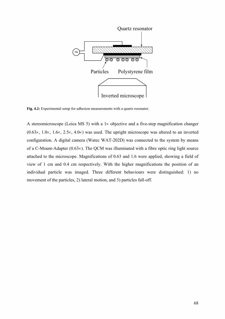
68
Polystyrene filmParticles
Quartz resonator
~
Inverted microscope
Fig. 4.2: Experimental setup for adhesion measurements with a quartz resonator.
A stereomicroscope (Leica MS 5) with a 1× objective and a five-step magnification changer
(0.63×, 1.0×, 1.6×, 2.5×, 4.0×) was used. The upright microscope was altered to an inverted
configuration. A digital camera (Watec WAT-202D) was connected to the system by means
of a C-Mount-Adapter (0.63×). The QCM was illuminated with a fibre optic ring light source
attached to the microscope. Magnifications of 0.63 and 1.6 were applied, showing a field of
view of 1 cm and 0.4 cm respectively. With the higher magnifications the position of an
individual particle was imaged. Three different behaviours were distinguished: 1) no
movement of the particles, 2) lateral motion, and 3) particles fall-off.

69
4.2 Materials and sample preparation
Borosilicate glass particles
Spherical borosilicate glass particles (Duke Scientific Corporation, California, USA) having
mean diameters of 5, 10, 15, and 20 ± 1 µm were used as received. Without taking the quartz
out from the holder, the particles were deposited on the polymer surface. For this purpose, a
thin metal-wire, washed before with THF and dried with nitrogen or left in a vacuum oven to
dry, was used to pick-up several hundreds of the particles from the bulk. They were placed on
the quartz surface by shaking. In order to deposit them in the center of the quartz, the particles
were deposited through a 1 mm diameter hole of an aluminium film used to cover the holder.
The smaller the particle-diameter was, the stronger the tendency of the particles to
agglomerate. For the 5 µm particles agglomeration was unavoidable while for 20 µm particles
practically no agglomeration was observed. The surface with deposited particles was imaged
by video camera connected to the microscope. In Fig. 4.3 representative images of particles
distribution on the quartz surface are shown. The images were analysed by Image Pro Plus
software (Media Cybernetics, Inc. Silver Spring, MD, USA) to determine the number of the
particles. The mean density of particles was 33200, 12900, 8700, 3200 particles per cm2 for 5,
10, 15 and 20 µm particles, respectively. The microsphere density is roughly 2500 kg/m3
(Duke Scientific Corporation data sheet).
Spin-coating
Spin-coating is widely used for producing thin layers, for example photoresist or
dielectric coatings, in the manufacture of microprocessors 106. In this method a small amount
of a diluted polymer solution is pippetted onto a spinning quartz. Excessive solution is flung
from the disc and the remaining layer thins as a result of centrifugal forces and evaporation.
The solution leaves behind a uniform polymer layer. Daughton and Givens 107 have reported
the final thickness to be independent of the volume of solution applied. Thickness of the
layers increases with the concentration and decreases with rotational rate.

70
Fig. 4.3: Representative video images of 5 (A), 10 (B), 15 (C) and 20 µm (D) diameter glass particles on
polystyrene films on a QCM.
Polystyrene films
Polystyrene (PS) with Mw = 11700 g/mol was dissolved in toluene (20 g/L). To remove
any dust, the solution was filtered through Millipore filters of 0.2 µm pore size (Millex
MILLIPORE, Syringe Driven Filter Unit, hydrophobic PTFE) before the polymer was spin
coated onto gold electrode at 1600 rpm for 60 s. Afterwards, samples were annealed for
15 min at 150oC in a preheated oven. After annealing, the quartz blank was left to cool down
to room temperature. As expected, after depositing a PS film on the gold electrode the
resonance frequency of the QCM decreased according to the mass density of the film. No
significant dependence of the resonance frequency on the driving amplitude was observed up
to amplitudes u0 of 10 nm (Fig. 4.4). For amplitudes between 10 and 16 nm a slight increases
of the resonance frequency was detected, which is small compared to the changes observed
due to the addition of particles. This frequency increase can be identified with nonlinearities
which occur at higher driving amplitudes. All experiments described, if not otherwise

71
mentioned, were performed at amplitudes < 10 nm, in order to eliminate the influence of
nonlinearities. When applying small amplitudes (≤0.5 nm) the partial slip is of negligible
influence. Furthermore loss of particles is also negligible, thus no frequency shift due to mass
loss is expected. Spectra recorded at low amplitudes should therefore reflect only changes
caused by different particle–bonding to the surface, as mentioned in Chapter 3.5.
1 10
-3000
-2000
-1000
0
Freq
uenc
y sh
ift (H
z)
Amplitude (nm)
Clean gold electrode
PS coated
Fig. 4.4: Resonance frequency versus amplitude at an excitation frequency of 18 MHz before and after forming a
polystyrene film of 157 nm thickness.
The film thickness was in the range of 100 – 180 nm as calculated from the QCM response
with the Sauerbrey equation Eq. 18. For a quartz thickness of dQ = 0.27 mm and quartz
density ρQ = 2650 kg/m3 the film thickness was calculated and compared to direct
measurements. These were taken by utilizing ellipsometry (Ellipsometer EP3 - SE, Nanofilm,
Germany) in order to verify the QCM results. The deviation was found to be less than
~ 30 nm, which is an acceptable result and suggest a good agreement between the two
methods (QCM vs. ellipsometry), considering the Sauerbrey model for QCM (described in
Chapter 2.2.3).

72
Surface qualitiy.
The quality of the gold electrodes and the surface coating was checked by atomic force
microscopy imaging in tapping mode. A detailed description of this specific methodology and
procedure is given in Chapter 6.

73
5. Results and discussion
5.1 QCM oscillation amplitude
In order to calculate the amplitude of the quartz crystal resonator motion, u0 (Fig. 5.1),
the Eq. 5 derived by Johannsmann 36 was applied, for which the effective amplitude, u0 is
given by:
02226
04
QUn
du
π= Eq. 70
here, d26 = 3.1×10⁻¹² m/V is piezoelectric strain coefficient, Q is the quality factor, n is the
overtone order (in this case n = 3), and U0 = 0.317×10(dBm/20) V is the driving voltage.
After spin coating the PS film on the electrode surface, the mean decrease of the amplitude is
in the order of 4 nm.
-20 -10 0 10 20
0.1
1
10
Ampl
itude
[nm
]
Drive level [dBm]
bare gold PS coated
Fig. 5.1: Amplitude vs. drive level for clean gold electrode and PS coated gold electrode.

74
5.2 Critical amplitude for particle detachment
In order to study the interaction between quartz crystal and particles, experiments were
performed over a wide amplitude range. Particle distribution on the surface, as well as
possible particle-detachment during oscillation, was observed by video microscopy. This
approach allowed to determine the amplitude value required to induce particle movement.
More precisely, depending on the applied amplitude, one could clearly distinguish between
three different behaviours: 1) no movement of the particles, 2) lateral motion (observed only
before annealing) and 3) particles falling off. The specific amplitude value leading to particle
detachment (3rd case) is defined here as the critical amplitude. Above this amplitude the mass
of the system changes and influences the measured frequency response significantly. The
experiments performed initially for studying the particle-surface coupling were done at
amplitudes much smaller than the critical one, thus ensuring that no particle-detachment took
place. In a different series of experiments, this specific critical amplitude for particle
detachment was determined for each system. Furthermore, surface changes occurred during
the particles movement were determined by AFM imaging and are described later in
Chapter 6.
Critical amplitude before annealing of PS-film
The amplitude required for loosing the primary bonding between particles and surface
for different quartz blanks was determined. The Fig. 5.2 shows results for different quartzes
and different particles sizes before annealing, when determining the oscillation amplitude at
which the first motion of particles occured. For very small particles (5 µm diameter), which
fell off at lower amplitudes, the differences between different quartzes were not significant.
The deviation of the critical amplitude was in the range of 1 nm (approximately 67% of the
mean value). The mean value of the critical amplitude was 1.5 nm. For 10 µm the mean value
was 3 nm, with a deviation ~ 2 nm (~ 67%). However, in the case of 15 µm diameter
particles, the deviation between single quartzes was very high, ~16 nm (above 100% of mean
value). As depicted in Fig. 5.2, for one quartz the particles fell off at an amplitude of approx.
4 nm, while in another case more than 20 nm amplitude had to be applied in order to simply
move the particles on the surface. The mean value of the critical amplitude was 10 nm.
Finally the mean value of the critical amplitude for 20 µm particles before annealing was 5
nm, with deviation ~ 2 nm.

75
0 2 4 6 8 10 12 14 16 18 20 22
5
10
15
20
size
[um
]
Amplitude [nm]
particles diameter 5 um 10 um 15 um 20 um
0.0 0.5 1.0 1.5 2.0 2.5
4.6
4.8
5.0
5.2
5.4
size
[um
]
Amplitude [nm]
particles diameter 5 um
Fig. 5.2: Critical amplitude before annealing. Size of the particles vs. driving amplitude – breaking of primary
bonding before annealing; Below, only the data for 5µm plotted for clarity.
Critical amplitude after annealing
After annealing at 1500C for 15min, the trend of the amplitude at particle detachment
did not change (see Fig. 5.3.). First the smallest particles were lost, i.e. 5 µm diameter by
mean critical amplitude 0.6 nm (deviation ± 0.5 nm). For 10 µm particles the mean critical
amplitude value was ~ 5 nm. The 15 µm particles started to move by 15 nm amplitude. For 10
and 15 µm particles the deviation in a range of 8 nm was measured. The broadest distribution
of amplitudes after annealing was found for 20 µm particles, with values between 2 and 18
nm and a mean of 8 nm.

76
0 2 4 6 8 10 12 14 16 18
5
10
15
20
size
[um
]
Amplitude [nm]
particles diameter 5 um 10 um 15 um 20 um
0.0 0.2 0.4 0.6 0.8 1.0 1.2
4.6
4.8
5.0
5.2
5.4
size
[um
]
Amplitude [nm]
particles diameter 5 um
Fig. 5.3: Upper: Critical amplitude after annealing. Size of the particles vs. driving amplitude necessary to break
the primary bonding after annealing; Lower: same data plotted at magnifified scale
When data before and after annealing are compared (Fig. 5.4.), it can be concluded that just
for 5 µm particles after annealing, the necessary amplitude to loose the particles from the
surface is lower than before. For the rest cases no such distinction can by made, thus the
deviation of 5 µm is not considered statistically significant.
These deviations of the singe values determined for particle detachement in every experiment
can be attributed to the different surface quality of each quartz-polymer film system used.
Furthermore, as already mentioned, one has always to consider a distribution of the

77
particle/surface coupling intensity. A certain fraction of the particles is detached. This amount
of detached particles depends on particle diameter and can be affected by the polymer film
quality and homogeneity. Another explanation is that, before annealing (rough surface), the
particle detaches when it meets a high resistance during its movement (as a ball rolling over a
“bumpy” road). After annealing, the particle settles in a meniscus of the surface. The
probability that it moves outside during its oscillatory movement is lower, however if this
takes place, the particle will also detach as easily as before.
0 2 4 6 8 10 12 14 16 18 20 22
4
6
8
10
12
14
16
18
20
size
[um
]
Amplitude [nm]
5 um before annealing 5 um after annealing 10 um before annealing 10 um after annealing 15 um before annealing 15 um after annealing 20 um before annealing 20 um after annealing
0.0 0.5 1.0 1.5 2.0 2.5 3.0
4
6
8
10
12
14
16
18
20
size
[um
]
Amplitude [nm]
5 um before annealing 5 um after annealing 10 um before annealing 10 um after annealing 15 um before annealing 15 um after annealing 20 um before annealing 20 um after annealing
Fig. 5.4: Upper: Critical amplitude. Size of the particles vs. driving amplitude before and after annealing; Lower:
same data plotted at magnified scale.

78
5.3 Contact between particles and polymer-film
To obtain more specific information on contact strength between particles and the PS
surface, the following experimental procedure was used: as a first step, the quartz was
characterized by a QCM frequency sweep directly after gold sputtering. In this way, the base
line to compare the changes in measured resonance frequency and to estimate the film
thickness was recorded. In a second step, a PS solution in toluene was prepared and the
polymer film was spin coated onto the quartz surface. The samples were annealed for 15 min
by 1500 C, in a preheated oven. After annealing, the sample was cooled-down to room
temperature. The data points for the bare PS film were recorded. In the following, all
frequency shifts are referenced to the PS-coated crystals prior to the deposition of spheres. In
the next step, particles were placed on the top of the quartz without taking it out from the
holder and the amplitude was slowly increased. The sweep - step was repeated at least three
times. Unless stated otherwise, the frequency shift ∆f was determined in the limit of small
amplitudes (< 0.5 nm) where partial slip is of negligible influence. Afterwards, the annealing
of the film with attached particles was performed for 15 min by 1500 C. The sample was
cooled-down to room temperature and the frequency shift measurements were repeated.
Finally, the surface was checked by AFM with respect to structural changes, utilizing the
tapping mode as described in Chapter 6.
20 µm particles
After the deposition of particles with a diameter of 20 µm on a PS coated surface the
measured resonance frequency always increased (Fig. 5.5.). From optical microscopy, the
areal number density N/AQ in the particular experiment shown in Fig. 4.3. was determined to
be about 30 particles/mm2.
Right after the first deposition of particles (Fig. 5.5, black squares) a ∆f of 350 Hz was
observed. Such an increase of the resonance frequency after addition of particles has been
observed before 30. This system is in the weak-coupling regime. Quantitative analysis of the
frequency shift with Eq. (58) yields a surprisingly high value for the spring constant, k.
Particle counting using video microscopy yielded a particle density N/AQ of the order of 30
particles/mm2. With ∆f ≈ 350 Hz (first sweep), Eq. (58) yields a spring constant of k ≈ 6000
N/m. This value can be compared to Hertz theory. The spring constant and the modulus are

79
given in Eq. 67, while the contact radius, a, as predicted from Hertz theory is derived in
Eq. 68.
In the following, the glass beads are taken to be much stiffer than polystyrene. In other words
the second terms in Eqs. 67 and 68 (G2 ≈ E2 ≈ ∞) are neglected. For polystyrene at MHz
frequencies, the shear modulus has been determined to be about 2 GPa 108. Inserting these
values, one finds a lateral spring constant of about 1000 N/m, which is a factor of 6 lower
than the experimental value. In order to match the experimental value of 6000 N/m, one
would have to use a shear modulus of 25 GPa, which is highly unrealistic. The contact radius
according to Hertz theory is 110 nm, used here for comparison reasons. This value is less than
the thickness of the polystyrene film. While the finite thickness may be of some influence in
principle, it is hard to see how the correction should amount to a factor of 6. Unexpectedly
high values for the spring constant as derived from Hertz theory have been found before 109.
The discrepancy has often surpassed a factor of 10. While there is no rigorous explanation at
hand, it can be suggested that the result can be understood on a qualitative level, assuming a
multiasperity contact.
In the first sweep, the oscillation amplitude was increased from u0 = 0.1 nm to 4 nm (to avoid
nonlinearities above ~10 nm). Video microscopy did not reveal significant movement of the
particles. Less than 5% of the particles fell off or moved on the surface. In the second sweep,
the resonance frequency increased by 2.5 kHz relative to the clean PS film. This indicates a
tighter coupling. This “consolidation” of the particle-PS contact can be interpreted in the
following way: Neither the particle nor the PS surface is perfectly homogeneous. During the
first sweep, the particles rotate and oscillate and in this way they obtain an optimum binding
position. In the third sweep (Fig. 5.5, red circles) only a slight decrease in the resonance
frequency was observed. No changes were detected by video microscopy, suggesting that the
mean coupling constant shifts back to slightly lower values during that sweep.

80
0 1 2 3 4-8.0
-6.0
-4.0
-2.0
0.0
2.0
∆f[
kHz]
Amplitude [nm]
1st
3rd
1st, annealedannealed,aged by atleast 6 sweeps
6λs
Fig. 5.5: Shifts of frequency versus amplitude of oscillation for the 20 µm particles. All spheres had been
deposited on a polystyrene film of thickness 160 ± 20 nm. Black squares show the first sweep after particle
deposition. Red circles show the third sweep after deposition. The oscillation of crystal has changed the nature of
the contact. Green upper triangle show the first sweep after high-temperature annealing of polystyrene film. The
negative frequency shift suggests increase of the contact strength. Blue lower triangles show results taken after
extended aging of these contacts. Higher oscillation amplitude has modified the nature of the contacts.
The fact that consolidation is a major effect was supported by the AFM adhesion force
measurements. Adhesion varied from one position to another by a factor of approximately 2-
3. Furthermore, the absolute value of 30-70 nN is relatively low. The model of Johnson,
Kendall, and Roberts 73 was utilized for an estimation of the adhesion. The adhesion force
between an elastic sphere and a planar surface is 3 2F WRπ= , where W is the work of
adhesion per unit area. With W = 0.03 N/m and F = 70 nN an effective radius of the sphere
can be estimated to be 0.5 µm. This is much lower than the actual radius and indicates that
surface roughness and particle inhomogeneities, as mentioned above, can lead to a
significantly reduced contact area.
The partial slip length is read from the ∆f-vs-amplitude by fitting a straight line to the
data at low amplitudes and extrapolating this line to ∆f = 0 according to Eq. 61. The dashed
lines at the top of Fig. 3.11 show these extrapolations. For the particles with 20 µm diameter,
the partial slip length is of the order of 0.6 nm. With an adhesion force of F⊥ = 1.1 µN and a

81
spring constant of k = 6000 N/m, one finds an apparent static friction coefficient of
µS ≈ F⊥/(kλS) ≈ 0.3. While this value is in the expected range, µS derived from λS and the
Mindlin model has occasionally also been found to be somewhat larger than unity 109. This
may well go back to a short-coming of the Mindlin model. However, a µS being larger than
unity may also be a consequence of the fast oscillation. This would imply, that the induction
of partial slip takes time and is less efficient at MHz frequency, than it would be in
conventional macroscopic experiments.
At this point one can contemplate the possibility of a rotation of the sphere under the
force of inertia. The Mindlin model assumes that the bulk of the sphere remains in rest. It
neither translates, nor rotates. Evidently, this is not fully realistic. One expects a slight
periodic rotatory component to the motion, in which case the presented experiments would
probe rolling friction rather than Mindlin microslip. The deformation pattern in the contact
zone would consist of a combination of shear and elongation, rather than pure shear. Finite
element calculations show that the amplitude of rotation is very small 110. The pattern of
deformation mostly is a shear deformation. However, if the moduli of the two contacting
materials are different, there still is a vertical stress component at the rim of the contact area.
This fact is well known from fracture mechanics 111. For a hard-soft contact, shear-induced
crack propagation always entails a normal tensile stress, termed „mode II crack opening“ in
this context. The essence of the Mindlin model (partial slip) certainly remains correct even for
mode II, concerning crack opening, but the details may need refinement.
After three sweeps on the QCM-particles system, the quartz crystal (including the
particles) was annealed at 150oC for 15 min in a preheated oven. After annealing and cooling
the frequency decreased to ∆f = 6.9 kHz (Fig. 5.5, green upper triangles). Following the
Dybwad model, one concludes that the contacts are now in the tight-coupling regime.
Annealing leads to the formation of a PS meniscus and binds the particles stronger to the
quartz. Meniscus formation was confirmed by atomic force microscopy (AFM). Under
control of an optical microscope a particle was removed from the surface with the tip of an
AFM. Subsequently, the PS surface was imaged in tapping mode. The dimensions of the
remaining menisci could be determined by AFM (Fig. 6.6).
Using the Sauerbrey equation, one can check whether the weight of the particles as
determined by QCM matches the number density from particle counting. The latter was 30
particles/mm2. If one assumes that the particles are tightly bound, the density of 26
particles/mm2 is calculated from Eq. 18. One could conclude that roughly 80% of the particles

82
are tightly bound to the QCM surface and follow its movement. In the framework of Fig. 3.8,
the system would be on the far left in the strong-coupling regime. However, it should be
pointed out that this is no unique conclusion. The system could also be in the intermediate
regime with k being slightly above the resonance point.
In the following sweeps leading to the aged state (blue lower triangles), the resonance
frequency gradually increased until the same state, as before temperature annealing, was
reached. This increase is interpreted as a reduction of the mean coupling constant. Actually,
the frequency shift remained below 4 kHz, as long as the amplitude sweeps did not exceed
3 nm. However, after several sweeps, it was observed that, for amplitudes above 4 nm the
frequency shift reached the level that the system exhibited before annealing (see Fig. 5.5).
After annealing no particle movement or detachment was detected by video micros-
copy, an observation which is in agreement with the negative frequency shift (for mass loss
one would expect an increasing ∆f) and excludes mass loss. However, as discussed in the
above paragraph, after “ageing” with repeating sweeps above a specific relatively large
amplitude (here 4 nm), the system retrieves the increased frequency shift values. Therefore it
is concluded that, if the amplitudes are high enough, the bond between the particles and the
PS surface can be reduced again to the level of the binding strength before annealing. With
decreasing mean coupling constant the system can go from negative frequency shifts in the
strong-coupling regime to positive frequency shifts in the weak-coupling regime.
15 µm particles
A similar positive frequency shift after particle deposition was observed with 15 µm
particles. In the example shown in Fig. 5.6, the frequency increased by 360 Hz upon addition
of particles. It further increased by 390 Hz in the second sweep. Afterwards, it remained
constant as long as the oscillation amplitude did not exceed 5 nm. No particle movement or
loss of particles was observed by video microscopy. Annealing caused ∆f to become negative
(1.9 kHz). As for the 20 µm particles, the decrease of the resonance frequency is attributed to
a tight coupling of the particles and the accompanying increase in effective mass. In contrast
to the larger particles, the resonance frequency did not change in all following sweeps, even
when increasing the amplitude to 10 nm. Video microscopy showed no indication of particle
movement or loss.
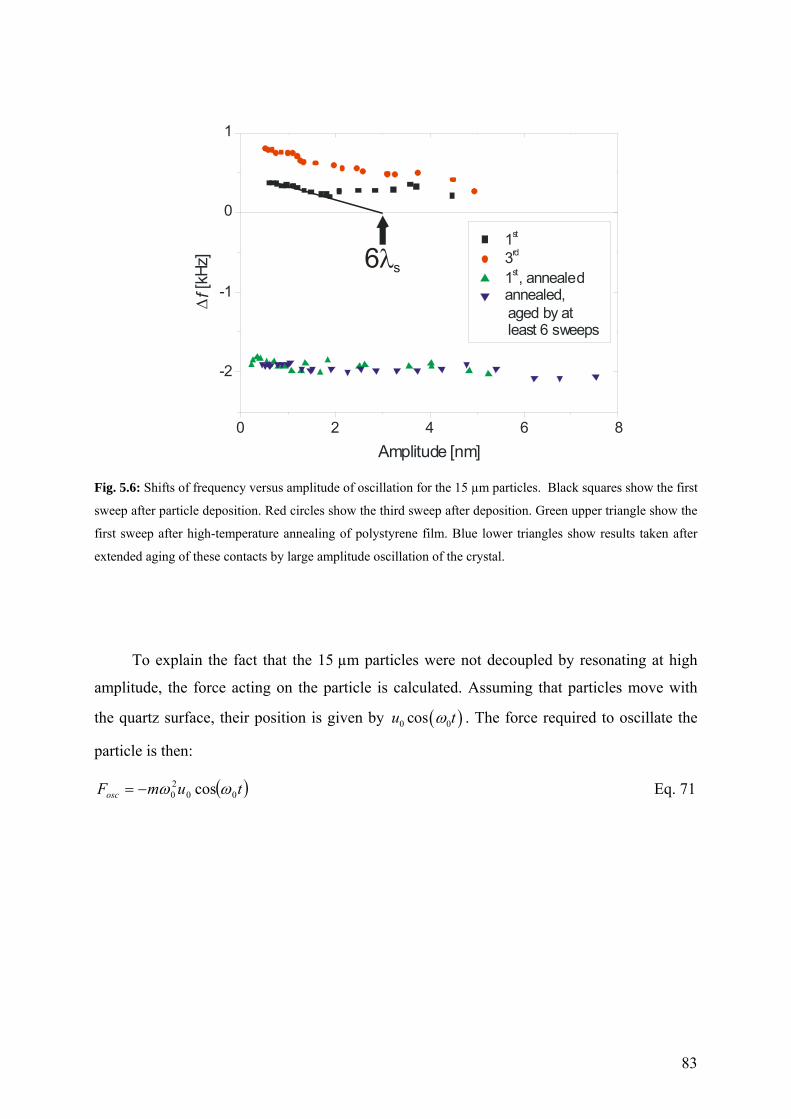
83
0 2 4 6 8
-2
-1
0
1
1st
3rd
1st, annealedannealed,aged by atleast 6 sweeps
∆f[
kHz]
Amplitude [nm]
6λs
Fig. 5.6: Shifts of frequency versus amplitude of oscillation for the 15 µm particles. Black squares show the first
sweep after particle deposition. Red circles show the third sweep after deposition. Green upper triangle show the
first sweep after high-temperature annealing of polystyrene film. Blue lower triangles show results taken after
extended aging of these contacts by large amplitude oscillation of the crystal.
To explain the fact that the 15 µm particles were not decoupled by resonating at high
amplitude, the force acting on the particle is calculated. Assuming that particles move with
the quartz surface, their position is given by ( )0 0cosu tω . The force required to oscillate the
particle is then:
( )tumFosc 0020 cos ωω−= Eq. 71

84
Crystal
Particle
PS film
RF
FR
a
h
Fig. 5.7: Schematic of a particle after annealing with a meniscus of PS.
The peak force is 3 20 04 3R uπ ρ ω . It increases with the third power of the particle radius.
This has to be compared to the force binding the particles to the surface. This binding force is
expected to grow proportional to R, though it is not clear how the binding between the particle
and the PS surface is broken. One might argue that in the absence of elastic strain the
adhesion force is proportional to the contact area. For a given film thickness with h R<< , the
contact area is approximately given by 2aπ , where a is the contact radius. Here, the influence
of the meniscus is neglected. With 2 22 2a hR h hR= − ≈ the contact area increases
proportionaly to R. Thus, the oscillation force due to the inertia of the particle increases with
R3 while the binding to the PS is expected to increase only with R. For large particles the
oscillation force is more likely to detach the particles, while for small particles the binding
force should dominate.
One might also argue via the torque. To detach the particle from its meniscus it would
need to roll up onto the film. The maximal torque leading to it is ( ) 3 20 04 3R h R uπ ρ ω− ⋅
4 20 04 3R uπ ρ ω≈ . Adhesion appears to resist to rolling. For a particle to roll, the torque adhaF
has to be overcome. Assuming that the adhesion force scales with the contact area, the
resistance is proportional to ( )3 23 2a hR= . Again, large particles should detach more easily
under an oscillating lateral force than small particles.
The experiments with the 15 µm particles revealed an intrinsic problem of the particle-
surface system, as described by the Dybwad model, which complicates the quantitative
interpretation of the results. Due to inertia effects, spheres of specific mass do not exactly

85
follow the oscillatory movement. Therefore do not contribute to the frequency shift as
expected from the Sauerbrey model. Within the semi quantitative model (Fig. 3.8), this is
explained by the system being in the intermediate regime between strong and weak coupling.
When k is around the resonance condition, ( k ≈ ω2m), a quantitative analysis is difficult and
this is probably the case with these specific particle-masses. Therefore, when comparing the
number of particles per unit area observed by microscopy with the mass per unit area derived
from the Sauerbrey equation, the latter is often found to be much smaller, due to the
phenomena described above (inertia, contact distribution and mean coupling constant
approximately in the resonance condition due to the particle mass). The difference for this
specific system amounted to up to a factor of 5.
10 µm particles
Deposition of 10 µm particles caused the frequency to increase by 280 Hz (Fig. 5.8,
black squares). Increasing the oscillation amplitude up to 5 nm caused no optical detectable
changes, although the frequency decreased by 75 Hz in the second sweep. The frequency shift
∆f remained stable after the second sweep. The red circles in Fig. 5.8 show the third sweep. In
contrast to the larger particles, annealing caused an increase of ∆f to a value of ∆f ≈ +450 Hz,
rather than a decrease. Evidently, annealing in this case was not sufficient to reach the strong-
coupling regime. Parameter k increased, pushing the system to towards the resonance
condition (thereby increasing ∆f). However, the increase did not carry the system beyond the
resonance condition.
Sweeps with a maximum amplitude of about 6 nm caused a further small increase of ∆f
by about 50 Hz. Increasing the amplitude to 10 nm caused particle loss and a decrease of ∆f
down to 285 Hz. Further increasing the amplitude to 16 nm left the sample unchanged.

86
0 2 4 6 80.0
0.1
0.2
0.3
0.4
0.5 1st
3rd
1st, annealedannealed,aged by atleast 6 sweeps
∆f[
kHz]
Amplitude [nm]
λs
Fig. 5.8: Shifts of frequency versus amplitude of oscillation for the 10 µm particles. Black squares show the first
sweep after particle deposition. Red circles show the third sweep after deposition. Green upper triangle show the
first sweep after high-temperature annealing of polystyrene film. Blue lower triangles show results taken after
extended aging of these contacts by oscillation of the crystal.
5 µm particles
When the smallest particles were added, a decrease of the frequency by ∆f ≈ -200 Hz was
observed (Fig. 5.9). Three amplitude sweeps did not change the frequency. After annealing,
the frequency decreased up to ∆f ≈ -400 Hz. Aging the sample at high amplitudes further
decreased the frequency down to -600 Hz. These particles were found to be in the strong-
coupling regime.
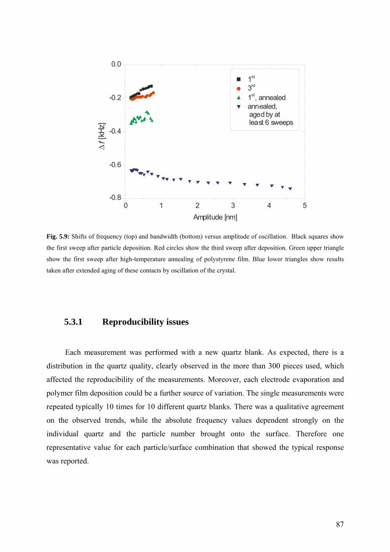
87
0 1 2 3 4 5-0.8
-0.6
-0.4
-0.2
0.0
1st
3rd
1st, annealedannealed,aged by atleast 6 sweeps
∆f[
kHz]
Amplitude [nm]
Fig. 5.9: Shifts of frequency (top) and bandwidth (bottom) versus amplitude of oscillation. Black squares show
the first sweep after particle deposition. Red circles show the third sweep after deposition. Green upper triangle
show the first sweep after high-temperature annealing of polystyrene film. Blue lower triangles show results
taken after extended aging of these contacts by oscillation of the crystal.
5.3.1 Reproducibility issues
Each measurement was performed with a new quartz blank. As expected, there is a
distribution in the quartz quality, clearly observed in the more than 300 pieces used, which
affected the reproducibility of the measurements. Moreover, each electrode evaporation and
polymer film deposition could be a further source of variation. The single measurements were
repeated typically 10 times for 10 different quartz blanks. There was a qualitative agreement
on the observed trends, while the absolute frequency values dependent strongly on the
individual quartz and the particle number brought onto the surface. Therefore one
representative value for each particle/surface combination that showed the typical response
was reported.

88
5.4 Effect of overtone order
The resonance of the quartz crystals was measured with a HP 5100A network analyser.
With this setup it is possible to excite and evaluate up to 20 overtones, depending on the
quality of the quartz blanks 51. These overtones are found at frequencies 0fnfn ×= with
12 += kn , k being an integer and f0 being the fundamental frequency.
As presented by Laschtisch 112 the amplitude decreases with increasing overtone order due to
the individual quality factors of each harmonic. The surface oscillation speed increases with
the overtone order, mainly from the first to the third harmonic, also due to the strongly
increasing quality factor, which is an expected behaviour. For each quartz however, the
quality factor of the harmonics increases with increasing overtone order.
In this section, the mechanical microcontacts of fine particles are studied using the quartz
crystal microbalance under oscillation and specifically focusing on the higher overtones.
While for the previous experiments the focus was in the 3rd harmonic, here the effects on the
higher harmonics (5th, 7th, 9th etc.) were additionally investigated. This is the first time that the
analysis of the higher harmonics is utilized for such a study with the quartz-crystal system and
it could provide with useful information for the particles movement and interaction with the
polymer surface. The experimental procedure and sample preparation are the same as for the
steps described in Chapter 4, with the only difference lying in the studied overtone (higher
overtones instead of only the 3rd).
The correlation between particle/surface contact and higher overtones was done here by
focusing on 5th and 7th overtone, of 30 and 42 MHz respectively. In order to have a defined
comparison with the other results, the 3rd harmonic at 18 MHz was also recorded. In each
experiment, the frequency shifts were measured for a stepwise increasing drive level. At each
applied drive level the above overtones were successively measured before moving to the
next higher amplitude value. As previously described, the particles were dry deposited on the
PS surface and for each measurement step three runs were recorded. The PS film was
annealed, by 150o C for 15 min, in order to influence the binding between particles and the
polymer surface.

89
5.4.1 Amplitude sweeps
The experiments had to be performed using very low amplitudes, in order to avoid
particle dislocation or detachment. The mass change was avoided in order to study only the
particle-surface interaction without any influence of particle-detachment on the recorded
frequency shifts. Therefore the drive level applied was between -20dBm and -10dBm. The
highest amplitude was detected for the 3rd overtone. As shown in Fig 5.10 for the PS coated
electrode it was in the range between 0.24 and 0.75nm. The particle deposition caused an
amplitude decrease, specifically for the 3rd overtone it was between 0.19 and 0.54 nm.
Through annealing the amplitude was further lowered to the level of 0.05 – 0.1 nm. In this
region the amplitude is not high enough to provoke particle movement on the surface.
Furthermore, it should not significantly influence the binding strength. Therefore, all
frequency shifts detected within this part of the study can be attributed solely to the applied
oscillation. Phenomena such as partial slip, particle-detachment and particle movement
(“jumping”) can be excluded.

90
-20 -18 -16 -14 -12 -10
0.1
0.2
0.3
0.4
0.5
0.6
0.7
0.8
Am
plitu
de [n
m]
Drive level [dBm]
3rd overtone 5th overtone 7th overtone
-20 -18 -16 -14 -12 -10
0.1
0.2
0.3
0.4
0.5
0.6
0.7
0.8
Am
plitu
de [n
m]
Drive level [dBm]
3rd overtone 5th overtone 7th overtone
Fig. 5.10: Amplitude for 3rd, 5th and 7th overtone for PS coated electrode (above) and after particle
(diameter 10µm) deposition (below). The amplitude level decreased significantly for all overtones.

91
5.4.2 Particles – surface interaction
5 µm particles
For the case of 5 µm particles the representative data for overtone comparison are
presented in Fig. 5.11. As mentioned above, the smallest particles, deposited on the PS coated
gold, caused for the 3rd overtone a frequency decrease, in this case by ∆f = -1553 Hz. Similar
behaviour was observed for the 5th overtone, where the frequency decrease was much
stronger, ∆f = -57379 Hz. The opposite effect was detected for the 7th overtone, where the
frequency increased by ∆f = +1085 Hz. As mentioned above, the amplitude range during
these experiments was very low (down to 0.05 nm) and no optical changes on the surface
were detected. Nevertheless, frequency shifts during each sweep for each overtone were
recorded. Specifically the driving amplitude was in the range of 0.04 – 0.12, 0.02 – 0.06, 0.04
– 0.12 nm for 3rd, 5th and 7th overtone respectively, for the 1st run before annealing. The
frequency shift as a function of the amplitude, D, during a sweep is defined as df(D) and was
also measured. For the 3rd overtone df(D) was approximately -100Hz to -200 Hz. The 5th
overtone frequency exhibited a df(D) = -30 to -50 Hz, while the 7th overtone actually
increased by df(D) = 20 – 40 Hz.
After annealing, the frequency decreased by -5367 Hz and -58958 Hz for 3rd and 5th overtone
respectively, using the clean PS film values as a reference. For the 7th overtone the frequency
increased by +3526 Hz. Additionally during these three sweeps no particle movement was
detected optically, however the frequency as a function of drive level for each sweep
increased by 350 – 500 Hz, 50 – 150 Hz, 50 – 110 Hz for the 3rd, 5th, 7th overtone
respectively.
The smallest particles exhibited a gradually decreasing frequency after deposition and after
annealing for the 3rd and 5th overtones, as expected. However, the 7th overtone exhibited a
deviating behaviour with a positive ∆f at both tests (before and after annealing). The same
contradiction was found for the frequency as a function of drive level at each sweep.

92
-20 -18 -16 -14 -12 -10-6000-4500-3000-1500
before annealing 1st run 2nd run 3rd run
after annealing 1st run 2nd run 3rd run
Drive Level [dBm]
3rd o
verto
ne
-59000-58000-57000-56000
5th o
verto
ne1000200030004000
7th o
verto
ne
Fig. 5.11: Frequency shift for 5µm particles by 3rd, 5th and 7th overtone before and after annealing with particles.
The 7th is the only overtone in this case exhibiting positive frequency shift.
10 µm particles
Deposition of 10 µm diameter particles caused the frequency increase by ∆f = +230,
+90, +33 Hz for 3rd, 5th and 7th overtone respectively (Fig. 5.12). The driving amplitude
before annealing was in the range of 0.19 – 0.54 (3rd), 0.07 – 0.22 (5th), 0.08 – 0.24 nm (7th).
During the measurement, the frequency as a function of drive level was not constant. For the
3rd overtone during a single sweep df(D) = -25 to -70 Hz, while for the 5th and 7th a minimal
frequency increase by 1 – 30 and 1- 20 Hz, respectively, was observed. During the whole
measurement process no particle movement was optically recorded.
In contrast to the other particles sizes, annealing caused an increase of the frequency for 3rd
overtone by +491 Hz relative to clean PS film, while for 5th and 7th overtone ∆f = –1713 and
- 5257 Hz respectively, as presented in Fig. 5.12. In agreement with the observations for the
5 µm particles, also in this case during each sweep, the frequency varied as a function of drive
level. For all three overtones df(D) during each sweep increased by 150 – 270 Hz, 50 – 70 Hz,
130 – 150 Hz for the 3rd, 5th and 7th overtone respectively.
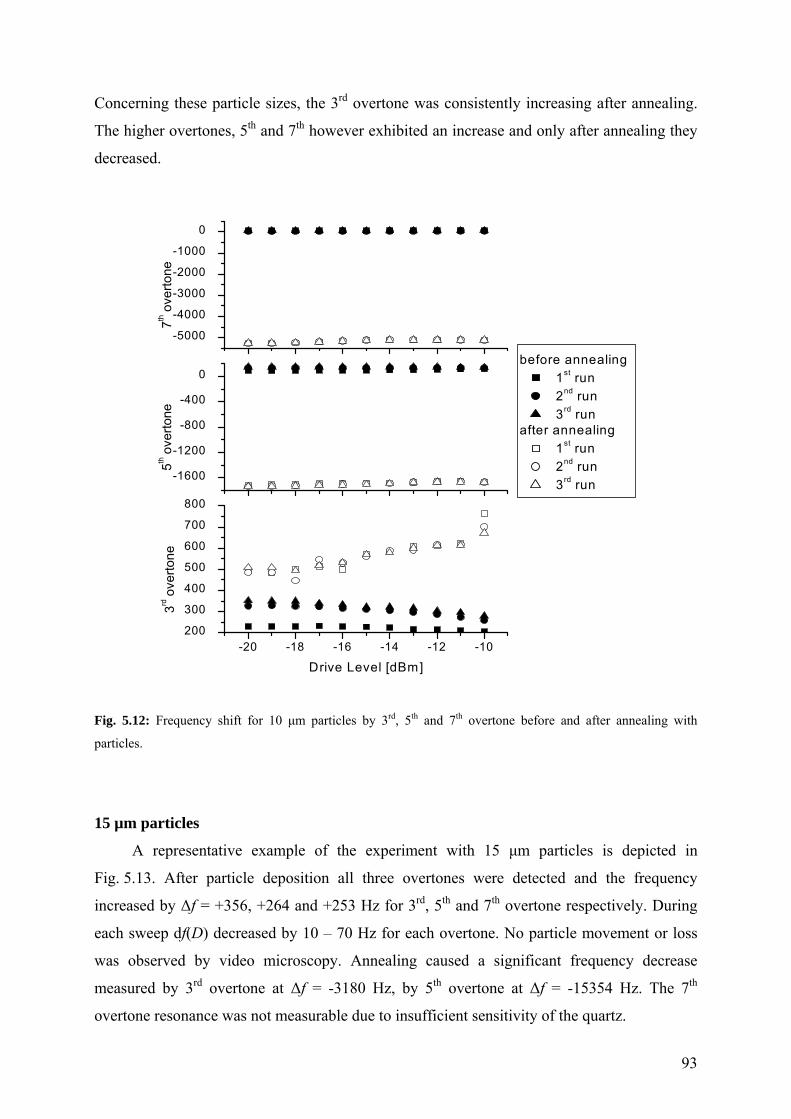
93
Concerning these particle sizes, the 3rd overtone was consistently increasing after annealing.
The higher overtones, 5th and 7th however exhibited an increase and only after annealing they
decreased.
-20 -18 -16 -14 -12 -10200
300
400
500
600
700
800
Drive Level [dBm]
3rd o
verto
ne
-1600
-1200
-800
-400
0
5th o
verto
ne
-5000
-4000
-3000
-2000
-1000
0
before annealing 1st run 2nd run 3rd run
after annealing 1st run 2nd run 3rd run
7th o
verto
ne
Fig. 5.12: Frequency shift for 10 µm particles by 3rd, 5th and 7th overtone before and after annealing with
particles.
15 µm particles
A representative example of the experiment with 15 µm particles is depicted in
Fig. 5.13. After particle deposition all three overtones were detected and the frequency
increased by ∆f = +356, +264 and +253 Hz for 3rd, 5th and 7th overtone respectively. During
each sweep df(D) decreased by 10 – 70 Hz for each overtone. No particle movement or loss
was observed by video microscopy. Annealing caused a significant frequency decrease
measured by 3rd overtone at ∆f = -3180 Hz, by 5th overtone at ∆f = -15354 Hz. The 7th
overtone resonance was not measurable due to insufficient sensitivity of the quartz.

94
For these larger particles, a frequency increase was observed before annealing and a
significant decrease afterwards. Both detected overtones exhibited the same trend for particle
deposition and annealing as well as during each individual sweep.
-20 -18 -16 -14 -12 -10
-3000
-2000
-1000
0
1000
Drive level [dBm]
3rd o
verto
ne
-16000
-12000
-8000
-4000
0
4000
5th o
verto
ne
220
230
240
250
260
before annealing 1st run 2nd run 3rd run
after annealing 1st run 2nd run 3rd run
7th o
verto
ne
Fig. 5.13: Frequency shift for 15 µm particles by 3rd, 5th and 7th overtone before annealing and after annealing.
After annealing resonance by 7th overtone was not measurable.
20 µm particles
After depositing the largest particles, 20 µm, on the polymer surface the resonance
frequency increased for all three overtones in the range of ∆f = 200 – 500 Hz (Fig 5.14). In
this case the frequency-change during single sweep before annealing was minimal, df(D) = 1
to 15 Hz. As in other cases, no particle movement was optically observed. After annealing,
the 5th overtone was not detectable, i.e. the resonance could not be found. For the 3rd overtone,
the frequency decreased by ∆f = -6857 Hz and the changes during single sweep were in the
range of 100 Hz. For the 7th the frequency increased by +9547 Hz and remained stable with
minimal changes of ~ 7 Hz.

95
As for 15 µm, the lowest resonance frequency, 3rd, exhibited a negative shift while the 7th
increased significantly. The measured shift was relatively constant over the applied amplitude
range for both recorded overtones, as well as before and after annealing. The mass of the
particles appears to be large enough to obtain a constant resonance value at each sweep.
However, the 7th overtone as before, appears to be affected by a different binding process than
the 3rd.
-20 -18 -16 -14 -12 -10-8000
-6000
-4000
-2000
0
2000
Drive level [dBm]
3rd o
verto
ne
290
295
300
305
310
5th o
verto
ne
0
2000
4000
6000
8000
10000
before annealing 1st run 2nd run 3rd run
after annealing 1st run 2nd run 3rd run
7th o
verto
ne
Fig. 5.14: Frequency shift for 20 µm particles by 3rd, 5th and 7th overtone before annealing, 3rd and 7th overtone
after annealing
Summarizing the results presented for different particle diameters, the frequency shift at
each overtone is relatively stable for the applied amplitude range. Minimal deviations are
demonstrated in the level of ±10 Hz. In general for small particles, i.e. < 15µm, the shift for
specific overtones can increase after annealing. For large particle diameters annealing causes
a frequency shift decrease observed at all overtones.
The QCM vibration can drastically change the micromechanical contact between the surface
and the attached particles. The oscillation can provoke the consolidation and enhancement of
the particle-surface coupling. However, for specific higher frequencies, one observes a break-

96
down of the contact. More specifically, for particles with 5 and 20 µm at higher overtones
(42 MHz, 7th harmonic) even very strong and stable particle-surface coupling can be
destroyed. The frequency shift after annealing is in both cases therefore positive, which
indicates that the system is in the weak-coupling regime. The opposite effect can be observed
in the case of 10 µm particles where at 5th and 7th overtone, the system enters the tight-
coupling regime and the frequency shifts are negative for these frequencies, indicating contact
consolidation.
Furthermore, as for the most cases of the 3rd harmonic, at the 5th overtone an enhancement of
the coupling between particle and surface is observed, after annealing. However, the
oscillation at the highest here studied overtone, the 7th, appears to break the contact and the
system enters the weak-coupling regime. The later happen for almost all particle diameters,
before and after annealing, indicating that the forces applied on the particles are much higher
than for the 5th overtone.
5.5 Calculation of particles per surface area
The number of particles on the active QCM surface can generally be estimated by
optical measurements or calculated using the Sauerbrey equation (Eq. 18). Optical analysis
was done for all particle sizes and the results were compared to the number of the particles
detected by the quartz frequency shift, ∆f. If the following assumption is made, that the
particles are tightly bound and effectively increase the mass on the quartz, their number can
be calculated from the frequency shifts, utilizing Eq. 18. The frequency shift value after
annealing was used. The above equation is applicable only for a negative frequency shift. For
the optical analysis of each quartz surface at least 30 images were taken and the mean
particle-density on polymer surface was estimated. The effective area is assumed to be equal
to the area of the small electrode (r = 0.35 cm, A = 0.38 cm2). In the table 5.1, the number of
the particles from imaging is compared to the calculated value for different overtones and the
deviation of each value calculated from ∆f to the quartz signal is attached.
A significant deviation is observed between the particle surface density microscopically
observed and values deduced from the QCM measurements. The agreement is good for the
largest particles. However, for the smallest particles, especially 5 µm, the surface density is by
far overestimated. The difference between values delivered by each overtone is also
significant. An example is the 15 µm case, where the 3rd underestimates while the 5th
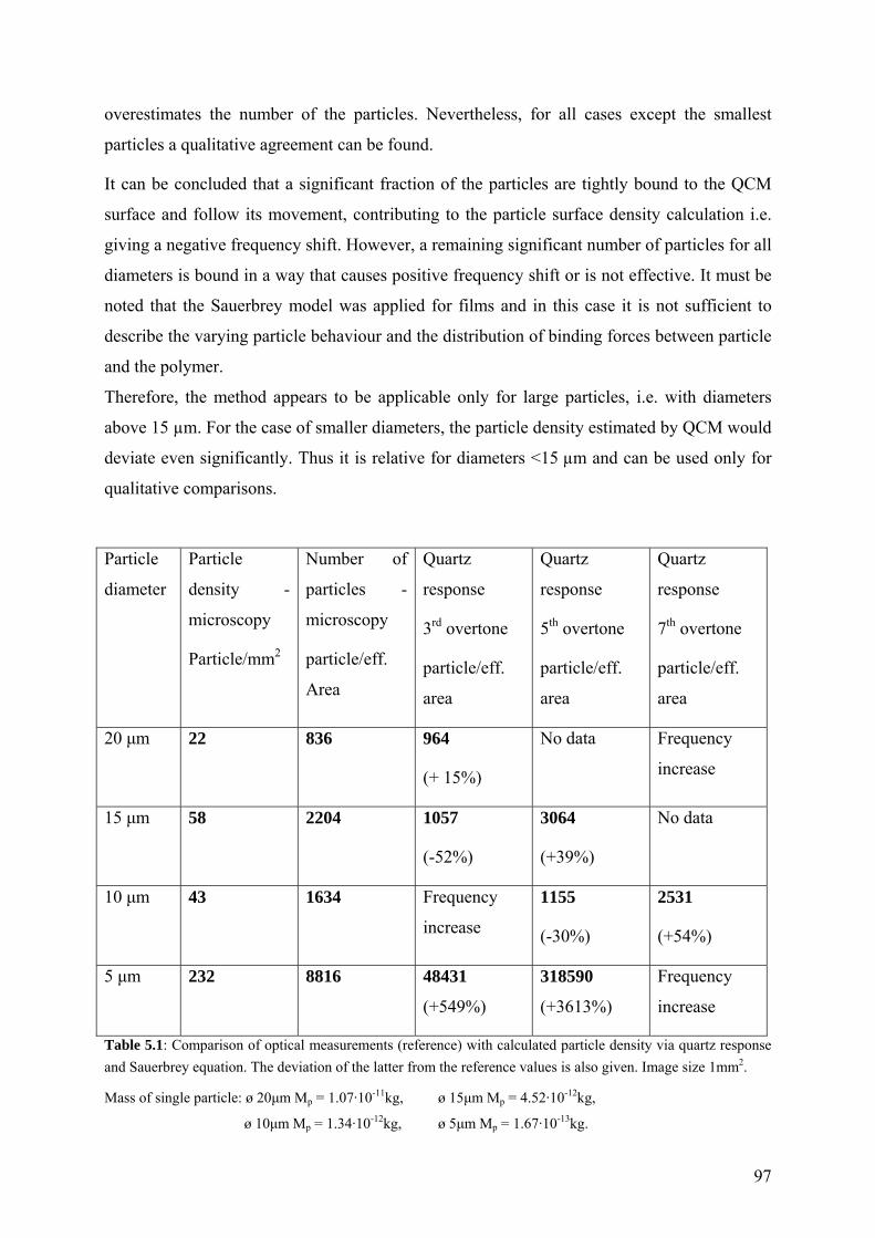
97
overestimates the number of the particles. Nevertheless, for all cases except the smallest
particles a qualitative agreement can be found.
It can be concluded that a significant fraction of the particles are tightly bound to the QCM
surface and follow its movement, contributing to the particle surface density calculation i.e.
giving a negative frequency shift. However, a remaining significant number of particles for all
diameters is bound in a way that causes positive frequency shift or is not effective. It must be
noted that the Sauerbrey model was applied for films and in this case it is not sufficient to
describe the varying particle behaviour and the distribution of binding forces between particle
and the polymer.
Therefore, the method appears to be applicable only for large particles, i.e. with diameters
above 15 µm. For the case of smaller diameters, the particle density estimated by QCM would
deviate even significantly. Thus it is relative for diameters <15 µm and can be used only for
qualitative comparisons.
Particle
diameter
Particle
density -
microscopy
Particle/mm2
Number of
particles -
microscopy
particle/eff.
Area
Quartz
response
3rd overtone
particle/eff.
area
Quartz
response
5th overtone
particle/eff.
area
Quartz
response
7th overtone
particle/eff.
area
20 µm 22 836 964
(+ 15%)
No data Frequency
increase
15 µm 58 2204
1057
(-52%)
3064
(+39%)
No data
10 µm 43 1634 Frequency
increase
1155
(-30%)
2531
(+54%)
5 µm 232 8816 48431
(+549%)
318590
(+3613%)
Frequency
increase
Table 5.1: Comparison of optical measurements (reference) with calculated particle density via quartz response and Sauerbrey equation. The deviation of the latter from the reference values is also given. Image size 1mm2.
Mass of single particle: ø 20µm Mp = 1.07·10-11kg, ø 15µm Mp = 4.52·10-12kg,
ø 10µm Mp = 1.34·10-12kg, ø 5µm Mp = 1.67·10-13kg.

98
6. Atomic Force Microscopy – Force Measurements and
Surface Imaging
Within this work, the Atomic Force Microscope (AFM) was used as a tool to image the
topography of the surface at high resolution and to measure force-versus-distance-curves. The
latter provided us with the range of adhesion force between particle and the surface. Knowing
the interaction forces between colloidal particles and surfaces is a precondition for
understanding the stability of dispersed systems and adhesion phenomena. In this chapter, the
use of AFM to measure directly the force between a planar surface and an individual colloid
particle is described. Therefore, a glass sphere was attached to the force sensor in the
microscope and the force between the particle and the surface was measured, under ambient
conditions. In the second part of this chapter, the surface changes occurring during quartz
oscillations are studied and analysed.
6.1 Force measurements – colloidal probe technique
A modified AFM probe can be used for direct measurements of colloidal forces. This
approach was presented by Ducker 67,68 et al. and Butt 69 and its application to adhesion force
measurement was reviewed by Kappl et al. 113. In this method a micron-sized particle, of well
defined spherical shape is glued to the end of an AFM cantilever, which serves as the force
sensor. This type of configuration allows direct force measurements. Additionally, the same
single particle, that is already attached to the AFM cantilever, can be used for further
experiments. In that case, the particle-surface should be examined after each
measurement/application and any contamination must be excluded before proceeding with the
next experiments. The accessible range of particle size is typically limited to a range between
1-50 µm 113. The measuring principle of the colloidal probe technique is otherwise identical to
that of a standard AFM as introduced in Chapter 3.2.1.

99
Particle attachment
In order to measure the adhesion force between particles and the polystyrene (PS)
coated surface using the colloid probe technique, borosilicate glass spheres with 10 µm
diameter were glued with epoxy glue (UHU plus endfest 300, UHU, Buehl, Germany) to the
end of AFM cantilevers (Schaefer Technologie, Langen, Germany, tipless rectangular silicon
cantilever, length 350 µm, 2.0 µm thick, resonant frequency 21 kHz). For securing the
placement of extremely small amount of glue and the colloidal particle in correct position,
onto the very end of the cantilever, a micromanipulator (three dimensional oil-hydraulic
manipulator MNO-203, Narishige Group, Japan) under the control of an optical microscope
was used.
Spring constant calibration
To evaluate the adhesion force value from the experimental data, the cantilever
deflection has to be multiplied with the spring constant of the cantilever. The spring constant
of the cantilevers was determined by the reference spring method introduced by Gibson et
al. 63 and Torii et al. 114. The reference cantilever was calibrated using the thermal noise
method introduced by Hutter and Bechhoefer 115. According to the reference spring method,
two cantilevers are used. The one is the ‘unknown’ with an attached sphere and the second
‘standard’ cantilever is calibrated by thermal tuning.
The ‘unknown’ cantilever was attached to a substrate, with the particle side up, and
pressed against the ‘standard’ lever, that is mounted in the sensor head of the AFM in the
normal configuration. In the first step, a force vs. distance curve with the ‘standard’ lever
being driven against a flat and hard surface (e.g. lever holder) is obtained. In the next step, the
end of the ‘standard’ cantilever is brought in contact with the end of the ‘unknown’ lever, see
Fig. 6.1. The series of force-distance curves are obtained in order to arrive at a representative
average value of the slope. Deflection of the ‘standard’ lever as a function of the z-height of
the stage is measured during the approach and retract cycles. Since the force constant, k0, of
the ‘standard’ lever is known, that of the ‘unknown’, k1, can be calculated from 63
( )[ ]1/01 −= NDCkk Eq. 72

100
where D is the z-height travel of the stage, C is the nV to nm conversion factor, and N is the
deflection (in nA) of the ‘unknown’ cantilever after contact.
Dk0k1
Laser DetectorN
Fig. 6.1: Schematic setup for spring constant calibration of the mass loaded cantilever. ‘Standard’ lever, k0,
‘unknown’ lever, k1, in their initial position, and after the sample stage has been moved a vertical distance D.
The deflection of the ‘unknown’ lever is N.
6.2 Adhesion force measurements
The adhesion force between borosilicate glass particle, with diameter of 10 µm attached
to the cantilever (Fig. 6.2) and polystyrene (PS) coated surface was measured. All results
were taken by using the so-called force-volume-mode. In this mode, forces-distance curves
are not only measured on one selected point of the sample, but are acquired in every point
corresponding to a pixel of the AFM image. Form the array of force-distance curves the
spatial variation of the interactions throughout the sample surface can be obtained 29. Within
this work the force curves were taken on a grid of 32 × 32 points, within a scan area of 500 ×
500 nm. The measured adhesion force for this system, Fadh, was in the rage between 30 – 70
nN depending on the position on the surface. A histogram of adhesion forces for the specific
system is shown in Fig. 6.3. Those data represent the value of measured adhesion force for the
same cantilever taken in three different positions on the same PS coated quartz crystal. As
expected this measurements shows a specific distribution of adhesion forces, rather than a
single value. For the estimation of the adhesion energy the theory of Johnson, Kendall, and

101
Roberts73 was applied in order to model the experimentally observed interactions (see
Chapter 3.5). The adhesion force between an elastic sphere and a planar surface
is 2/3 WRF π= , where W is the work of adhesion per unit area. Assuming a typical value of
W = 0.03 N/m for polymer surfaces and the measured adhesion force F = 70 nN an effective
radius of the sphere would result in R = 0.5 µm. This is much lower than the actual particle
radius and indicates that the surface roughness reduced the contact area significantly. If the
actual particle radius is used in the above relation (R is set to 5µm), then from the maximum
measured force of 70 nN, one would calculate a work of adhesion as low as W = 0.003 N/m,
which is far too small for the specific system.
The influence of surface roughness and surface heterogeneity on variation of force value
was investigated and reported by several research groups 22,23,25-27,116. Roughness can cause a
significant change in the contact area of two particles, depending on the location of this
contact. Heterogeneity in chemical composition or molecular structure, at different length
scales can cause a different energy of adhesion and thus a variation in the effective adhesion
force, depending on the precise contact location. Nevertheless, for this specific system,
roughness can only partially reduce the work of adhesion and is not the only factor for the
almost 10-times lower W calculated compared to the expected values.
10µm10µm
Fig. 6.2: SEM image of borosilicate glass particle attached to the cantilever

102
-80 -60 -40 -20 00
50
100
150
200
250
300
350
400
450
500
550
Num
ber
Adhesion force [nN]
position 1 position 2 position 3
-80 -70 -60 -50 -40 -30 -20 -100
200
400
600
800
1000
1200
1400
1600
Num
ber
Adhesion force (nN)
Fig. 6.3: Histogram of the distribution adhesion forces for one cantilever in 3 positions on the PS surface. On the
right side the average values of the measurements at all three positions are plotted.
6.3 Surface changes caused by particles - Surface Imaging
In the previous paragraphs, the method of measuring forces with the AFM was presented.
Moreover, the AFM technique can be utilized in order to determine surface topography, i.e.
quality and possible surface changes from interactions. These can be quantified with the AFM
in two commonly used modes, which are briefly presented in the Chapter 3.2.1.
6.3.1 Surface quality
AFM imaging in tapping mode (Dimension 3100, Veeco Instruments, cantilever tapping
mode, OMLCLAC 160 TS-W2, Silicon) was used during this work to measure the roughness
of the quartz surface. Surface roughness is one of the factors describing the surface quality
and the influence on the interaction between particles and surface. Further factors of surface
quality, which are less important for this system, can be the chemical homogeneity and
density fluctuations. Firstly, the quality of gold electrodes was determined and an average
root-mean-square (rms) roughness of σrms = 1.1 nm or below over an area of 5 x 5 µm2 was
found, which is quite low. Secondly, polystyrene (PS) coated gold electrodes were imaged
and a mean rms roughness of 0.78 nm over an area of 5 x 5 µm2 was found, confirming the
good surface quality with relatively low roughness.

103
6.3.2 Surface damage by the particles
Within this section, the surface changes occurring during quartz oscillations are
described. When the particles follow the QCM surface movement, the forces reach values that
can be calculated by 20rF m Aω= , where m is the particle mass, ωr is the resonance frequency
and A0 the amplitude. For the 20 µm particles, with m = 10 ng, ωr = 113 MHz, and A0 ≈ 20
nm peak forces are calculated to reach 2.7 mN. This can lead to high local stresses in the
polymer. Assuming a contact area of 1 µm2 for example, leads to an applied pressure of
3 GPa. Such a pressure may lead to irreversible deformation of the polymer surface. For this
reason, by utilizing AFM the polymer film was investigated, regarding deformation that are
attributed to the glass particle movement takes place. The particle was removed from the
surface using an AFM tip. The particle detachment using the AFM setup was simultaneously
monitored with an optical microscope. Subsequently, the PS surface was imaged in tapping
mode and the detected particle traces were quantified.
As a first control, particles were placed on an annealed PS coated surface without quartz
oscillation. After 24 h the particles were carefully removed with the help of the cantilever and
the surface was directly afterwards imaged with the AFM tapping-mode technique. It was
observed that the particles left barely visible marks on the surface. The picture in Fig. 6.4
depicts an example of the imprint left by a 20 µm particle. The diameter of this mark was
0.6 µm with a depth of less than 10 nm. The fact that such structures, which are quite small
compared to the particle diameter, could be found after the particle-removal is surprising.
Nevertheless, there was no doubt that this is an imprint of a particle on the surface, since these
structures were repeatedly detected.

104
110 nm
0.0 nm
15 nm
Fig. 6.4: Structural changes on the PS coated gold before quartz oscillation and after removing a 20 µm particle.
After resonating the quartz up to the amplitude where the particles started to move and
change their position, the structural changes induced at the film surface were detected
(Fig. 6.5). Different kinds of marks were observed, suggesting that the particle-behaviour was
heterogeneous. In some cases, the particles remained at their lateral position and formed an
imprint at that point (Fig. 6.5a). In other cases, several such repeating imprints side-by-side
and partially overlapping were observed (Fig. 6.5b). The particle seemed to have jumped from
one position to the next but stayed at every position for many vibrations of the QCM. Finally,
several particles appeared to have “jumped” at every vibration of the QCM so that periodic
marks were left in the PS film, which should be correlated with the QCM frequency (Fig.
6.5c).

105
Scanning size 10 mµ 5 mµ3 mµ
3 0 n m
0 . 0
5 0 n m
0 . 0
Fig. 6.5 (a – c): AFM image of surface changes after quartz stimulation with 20 µm particles. a) circular prints
after particle detachment with diameters - ~1.3µm, depth ~ 20nm, occurring for less than 50% of the particles. b,
c) dislocation of the particle on the surface, occurred for less than 3% of the particles
These particular traces allowed us to estimate particle velocity during the quartz
oscillation. In the example shown in Fig. 6.5c, the 20 µm particle needed 6 periods in order to
move 3 µm. At a frequency of 18 MHz that leads to an escape velocity of 9 m/s. Assuming
that the particle was trapped at the upper right mark for many periods it had to accelerate to
the speed of 9 m/s within one half period (28 ns). To achieve the corresponding acceleration
of 3.2×10⁸ m/s2 a minimal force of 3.5 mN is required. This force magnitude is in agreement
with the above estimation of the forces acting on the particles. Structural changes, as shown in
Fig. 6.5, were observed for 10 - 20 µm particles. Only the smallest 5 µm particles left no
structural changes, at least not within the applied amplitude range.
An alternative explanation, which leads to a lower estimate for the horizontal velocity,
vh has to be also mentioned. Due to the vibration of the QCM the particle is not only accele-
rated horizontally but also vertically. Considering that it has to overcome the polystyrene
meniscus it is reasonable to assume that a vertical component, vv, is present. Like a stone
thrown at grazing angle over water the particle might jump up and down while moving
laterally over the polystyrene surface. The force attracting it back to the surface is the van der
Waals force. At each touch of the surface an imprint is left behind due to the vibrating QCM
surface. In order to estimate the lateral velocity of the particle, the time for one jump has to be
determined first. The vertical velocity has to be lower than the escape velocity. The escape
velocity is the velocity of the particle which would allow it to escape the van der Waals
attraction. Setting the potential van der Waals energy of the particles in contact with the
surface, 06HA R D , equal to the kinetic energy required to leave the surface, 2 2emv with
34 3m Rπ ρ= , an escape velocity is obtained from the following relationship:

106
Eq. 73
With typical values for the parameters (AH = 2×10-20 J, D0 = 0.17 nm, ρ = 2500 kg/m3) a value
of ve ≈ 6 mm/s is derived. In the present set of experiments the particles fall off once
gravitation is stronger than the van der Waals forces. For a particle radius of 10 µm a fall-off
distance of D = 18 nm is obtained. The time of one jump can be estimated to be eD vτ = ≈
3 µs. With a spacing of 0.5 µm (6 “particle-jumps” in a distance of 3µm) between the
elongated marks on the surface, the horizontal velocity is estimated to be approximately
0.16 m/s.
6.3.3 Meniscus formation
The final step in the surface characterisation was to obtain images after annealing with
particles on the PS coated electrode, thus confirming the meniscus formation. The particles
were removed by an AFM cantilever and a microscope camera allowed their detection. The
removal was carefully performed and controlled in order to minimize the destruction of the
meniscus and leave the rim unaffected. Nevertheless, for some cases the particle was strongly
bonded to the film, thus causing rim damage during removal and detachment. However this
was easily detectable and taken into consideration. An alternative method of particle removal
is difficult to apply, because the position of the removed particle has to be exactly defined for
the AFM image. For the majority of the particle/surface contacts, this method did not
significantly change the shape of the meniscus.
Three main types of meniscus shape were detected. The first was a symmetric imprint of a
radius which corresponded to a full particle/polymer contact area. This is demonstrated in Fig.
6.6 and 6.7, where one can assume that the particle was tightly bound and the meniscus
dimensions were correlated to the particle diameter. Figure 6.6 shows an example of the
meniscus formed by a 10 µm particle. Similar structural changes were imaged for all particle
sizes, e.g. for 20 µm as demonstrated in 6.7. The meniscus created was 80 – 130 nm deep and
the diameter was in the range of 3 to 6 µm, dependent from the particle size.
0
14
He
Av
R D=
πρ
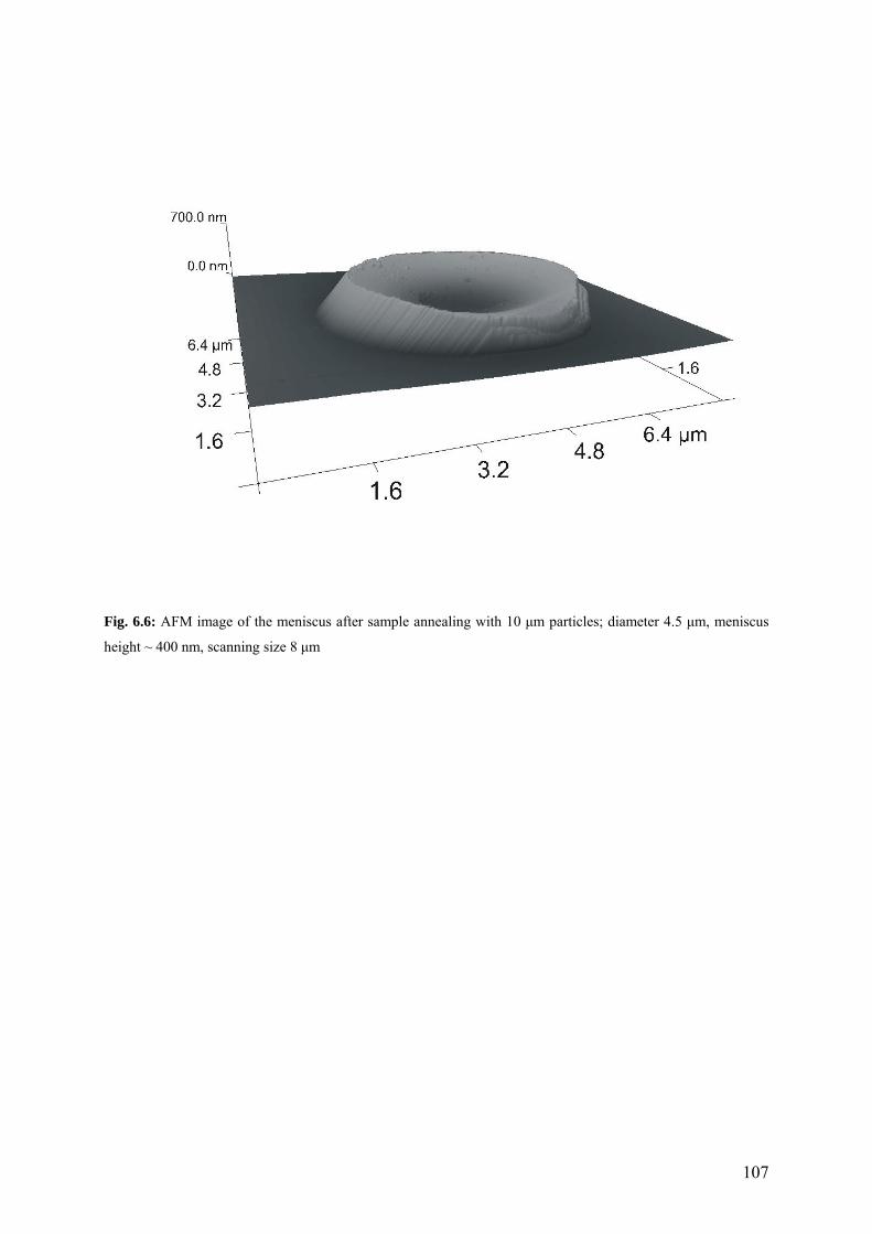
107
Fig. 6.6: AFM image of the meniscus after sample annealing with 10 µm particles; diameter 4.5 µm, meniscus
height ~ 400 nm, scanning size 8 µm

108
600 nm
0.0 nm -1 0 1 2 3 4 5 6 7 8
-100
-50
0
50
100
150
200
[nm
]
[µm]
-5 0 5 100
4000
8000
12000
16000
R = 10µm
[µm]
[nm
]
-5
0
5
10
15
Fig. 6.7: Upper left: an AFM image of a meniscus created by a 20 µm particle, after 5 min annealing by 1600C.
Upper right: the cross-section of the depicted meniscus (red line in the left picture). Lower: Representation of the
particle-surface meniscus contact on µm scale.

109
The second type was an asymmetric meniscus, with one “side” higher than the other, as
shown in Fig. 6.8. In addition, the imprint exhibited additionally a plateau. The latter is a
“flat” area in the center of the particle position on the surface with a diameter of
approximately 2 µm. This is however not to be confused to a damaged rim due to particle
removal but it is clearly due to an irregular inhomogeneous meniscus development. This
could be attributed in e.g. film inhomogeneity. A complete penetration of the film by the
particle in this case is excluded and the observed plateau is indeed a polymer surface. In case
a mechanical destruction of the meniscus during the manual particle removement would take
place, the meniscus rim would be obviously and clearly interrupted and broken, as
demonstrated in Fig. 6.7.
800 nm
0.0 nm
-2 0 2 4 6 8 10 12 14 16
-100
-50
0
50
100
150
200
250
[nm
]
[µm]
Fig. 6.8: Left: Asymmetric meniscus formed from a 10 µm particle on the surface after 15 min annealing by
1600C. Right: Cross-section of the depicted meniscus (line with red-points in the left picture).

110
The third type of meniscus shape was a relatively symmetrical form including a smaller
symmetrical meniscus in the centre, presented in Fig. 6.9, 6.10. In the middle of the meniscus
the contact point between the particle and the PS film could be recognised and imaged, which
resembles a very small plateau of 2 µm diameter. A smaller meniscus appears to be formed in
the middle of the main meniscus.
700nm
0.0nm
1000
0.0
0 2 4 6 8 10-150
-100
-50
0
50
100
150
nm
µm
Fig. 6.9: Height (upper left) and phase (upper right) images of the meniscus formed by a 15 µm particle on the
PS surface after 15 min annealing. The smaller homocentric meniscus is clearly depicted and regarded as the
effective contact area. In the lower figure this is also clearly demonstrated in the plot of the cross-section and the
approximately 1µm diameter secondary meniscus.

111
700nm
0.0nm
300
0.0
0 1 2 3 4 5-80
-60
-40
-20
0
20
40
60
80
100
120
high
t [nm
]
[um]
Fig. 6.10: Height (upper left) and phase (upper right) images of the meniscus formed from a 5 µm particle on the
surface after 15 min annealing. The smaller homocentric meniscus is clearly depicted and regarded as the
effective contact area. Scan size 5 µm. Below the cross-section with the secondary meniscus of approximately
1µm diameter depicted.
When zooming in on the centre of the meniscus spot, one could recognise that the
particles were definitely in contact with a very thin polymer layer and did not yet touch the
quartz electrode surface. This is demonstrated for the inner smaller meniscus of Fig. 6.10
which is shown in more detail in Fig. 6.11. This layer has a significantly higher roughness
than the original polymer surface, which appears to be qualitatively similar to the roughness
of the particle surface. Hence, it could be suggested that the observed surface of the secondary
meniscus is a direct imprint of the particle.

112
The images in Fig. 6.9 and 6.10 can be explained in the following way: The effective
particle-surface contact is the secondary meniscus of the small diameter of approx. 1µm
diameter. The larger meniscus of a diameter 4-6 µm stabilizes the particle during oscillation
and keeps it in position. This smaller meniscus would be the case of a weak particle-surface
coupling, while for strong-coupling the particle would be expected to have a “full meniscus”
contact area with the film.
400
300nm
0.0nm 0.0
Fig. 6.11: Height (left) and phase (right) zoom in on the centre of Fig. 6.10: Secondary meniscus after annealing
of 15 µm particle for 15 min, height and phase image, scan size 1.7 µm.
Additionally, the influence of annealing time on the meniscus formation was studied.
From AFM images for samples after different annealing durations, it was determined that
2 min is adequate to fully form the structure. The structure remains unchanged under further
annealing, specifically at typically 15 to 60 min. If however, the annealing takes place for
over than ~100 min the film is degraded and “dissolves” close to the meniscus, in other words
a dewetting of the film takes place, which is significantly affected and reduced in height. An
example of this defect is shown in Fig. 6.12.
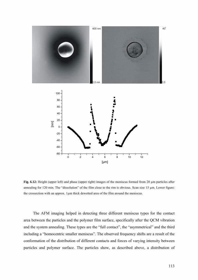
113
400
0.0
400 nm
0.0 nm
0 2 4 6 8 10 12-80
-60
-40
-20
0
20
40
60
80
100
[nm
]
[µm]
Fig. 6.12: Height (upper left) and phase (upper right) images of the meniscus formed from 20 µm particles after
annealing for 120 min. The “dissolution” of the film close to the rim is obvious. Scan size 15 µm. Lower figure:
the crossection with an approx. 1µm thick dewetted area of the film around the meniscus.
The AFM imaging helped in detecting three different meniscus types for the contact
area between the particles and the polymer film surface, specifically after the QCM vibration
and the system annealing. These types are the “full contact”, the “asymmetrical” and the third
including a “homocentric smaller meniscus”. The observed frequency shifts are a result of the
conformation of the distribution of different contacts and forces of varying intensity between
particles and polymer surface. The particles show, as described above, a distribution of

114
coupling-constants rather than a single precise value, while the system can find itself in the
strong- or in the weak-coupling regime.
All three meniscus types can be detected for all 4 particle sizes studied, even within the
same sample. They appear after annealing and have reproducible dimensions, in agreement
with the contact surface that is assumed for the specific particles on the polymer film. The
different bonding intensity, to which the meniscus forms are attributed, could explain the
deviation between number of particles per surface area measured by imaging and the values
provided by the QCM via the frequency shift analysis. One assumption could be that, the
asymmetric and the homocentric contact types are responsible for the positive frequency
shifts observed for the 3 measured overtones, in other words for the weak-coupling regime in
which the system appears to be. The particles with this binding intensity would change their
position faster and would not necessarily follow the QCM movement. Thus, they would not
effectively contribute to the mass increase of the quartz. The latter case is quantified by the
negative frequency shift, ∆f < 0 and can be the outcome of a “full contact” between particle
and polymer film surface.

115
7. Summary and conclusions
The particle-surface contact is important for a wide range of industrial applications and
governed by micromechanics. Within this work, a new methodology is developed for
measuring adhesion forces, which utilizes the quartz crystal microbalance, QCM, and
implements it for studying particle-polymer film interactions. The potential of this technique
in measuring forces in this type of systems is evaluated by carrying out experiments with
particles of different diameters, under different conditions. Furthermore, imaging and atomic
force microscopy, AFM, is additionally utilized in order to validate the results and analyse
how QCM experiments reflect the state of adhesion.
The quartz crystal microbalance is a very sensitive method developed to measure the
mass per unit area of homogeneous thin films. Within this work, it is extended to study the
contact between glass particles and a polymer, i.e. polystyrene, surface. The experimental
setup consists of the QCM with the polymer film deposited onto the quartz surface. The
imaging is performed by an optical microscope in order to get a combined monitoring of the
phenomena taking place during the vibration. With this setup it is possible to monitor the
particle motion under oscillation, while attached to the surface. The resonance frequency shift
recorded is reproducible and used to quantify the stiffness of the polymer-particle contact.
This interaction is found to be governed by the interplay between inertia and contact forces.
The induced frequency shift is found to decrease or increase, depending on the type of
particle-surface coupling and the amplitude and frequency overtone of the oscillation.
For a deeper understanding of the observed phenomena, four general models are taken
into consideration, i.e. the Hertz, Johnson-Kendall-Roberts, Derjaguin-Müller-Toporov and
the Mindlin theory of partial slip. The latter is utilized in order to qualitatively interpret the
resulting frequency shifts and the estimated adhesion forces and particle velocities.
Considering the above theories and the resulting frequency shifts of the 3rd overtone in
the QCM, one can describe the interaction between the particles and the surface. For strong
coupling with the QCM surface, the particles appear to move with the vibrations and simply
act as added effective mass. This leads to a decrease of the resonance frequency, in agreement
with the Sauerbrey equation (calculation of added mass on QCM). However, when the system
enters a regime of weak coupling between surface and particles, the latter are not able to
follow the fast movement of the QCM surface. Hence, they effectively act as adding a

116
“spring” with an additional coupling constant and increase the resonance frequency. This
positive frequency shift was consistently observed and was qualitatively reproducible.
When the QCM vibrations exceed specific critical amplitude, they may even lead to
particle detachment. This critical amplitude was determined for the system using amplitude
sweeps. During this set of experiments, three different behaviours were observed: no
movement of particles at very low amplitudes, lateral motion at intermediate amplitudes and
finally detachment, above the critical value. In experiments probing the particle – surface
coupling, only amplitudes well below the critical one were applied in order to avoid
frequency changes due to mass loss, as described by the Sauerbrey theory.
Furthermore, the higher overtones, specifically the 5th and the 7th were utilized in order
to derive, if possible, additional information about the interactions taking place. In general,
for small particles, i.e. < 15µm, the shift for specific overtones can increase after annealing.
For large particle diameters annealing causes a negative frequency shift at all three higher
overtones. For specific higher frequencies, one observes a break-down of the contact and even
very strong and stable particle-surface coupling can be destroyed. The shifts at the lower
overtones describe a generally strong-coupling regime for the system. For the highest
overtone however, 7th, a break-down of the contact was observed, indicated by positive
frequency shifts for most of the studied particles.
The applicability of the QCM method for quantifying particle-surface interactions and
directly measuring adhesion forces is investigated. In the analysis, one has to take into
account that the particles show a distribution of coupling constants rather than a single,
precisely defined value. When this distribution is convoluted with the model-predicted
frequency shift ∆f, three regimes can be distinguished: (1) For low mean coupling constants
k , the frequency increases with increasing k until it reaches a maximum. (2) After the maxi-
mum ∆f decreases and turns negative to reach a minimum. (3) Further increasing k leads to a
gradual increase of ∆f until it has reached a value in which the mass increase dominates. It is
found that, solely from standard QCM experiments, a quantitative determination of
interaction forces of particles with surfaces does not seem to be possible. One reason is that
the frequency shift is not a unique function of the coupling constant. Therefore, the value of
adhesion force cannot be deduced from the frequency shift measured by the QCM system.
Finally, the AFM method is introduced and used as a complementary method for direct
force measurements. AFM is further applied in order to study the surface of the polymer film
after the system excitation and removement of the particles. The AFM imaging helped in

117
detecting three different meniscus types for the contact area between the particles and the
polymer film surface, specifically after the QCM vibration and the system annealing. These
types are the “full contact”, the “asymmetrical” and the third including a “homocentric
smaller meniscus”. The observed frequency shifts are a result of the conformation of the
distribution of different contacts and forces of varying intensity between particles and
polymer surface. All three types of surface structures can be detected for all 4 particle sizes
studied, even within the same sample under investigation. The different bonding intensity, to
which the meniscus forms are attributed, could explain the deviation between number of
particles per surface area measured by imaging and the values provided by the QCM via the
frequency shift analysis. The asymmetric and the homocentric contact types are suggested to
be responsible for the positive frequency shifts observed for the 3 measured overtones, in
other words for the weak-coupling regime in which the system appears to be. The particles
with this binding intensity would change their position faster and would not necessarily
follow the QCM movement. Thus, they would not effectively contribute to the mass increase
of the quartz. The latter case is quantified by the negative frequency shift, ∆f < 0 and can be
the outcome of a “full contact” between particle and polymer film-surface.
The AFM provides is utilized here to study the surface effects and more importantly to
quantify the forces between particles and surface, while QCM gives qualitative information
on the contact type and interaction intensity.

118
References
1 J. N. Israelachvili, Intermolecular and Surface Forces, 2 ed. (Academic Press,
London, 1992). 2 M. A. Felicetti, G. R. Salazar-Banda, J. R. Coury, and M. L. Aguiar, Industrial &
Engineering Chemistry Research 48, 877-887 (2009). 3 G. R. Salazar-Banda, M. A. Felicetti, J. A. S. Goncalves, J. R. Coury, and M. L.
Aguiar, Powder Technology 173, 107-117 (2007). 4 R. Polke, Bull. Soc. Special Chim. France A3241, 51-54 (1969). 5 R. Polke, Chemie Ingenieur Technik 40, 1057-& (1968). 6 S. W. Booth and J. M. Newton, Journal Of Pharmacy And Pharmacology 39, 679-684
(1987). 7 K. K. Lam and J. M. Newton, Powder Technology 65, 167-175 (1991). 8 K. K. Lam and J. M. Newton, Powder Technology 73, 117-125 (1992). 9 K. K. Lam and J. M. Newton, Powder Technology 76, 149-154 (1993). 10 S. H. Kim, D. B. Asay, and M. T. Dugger, Nano Today 2, 22-29 (2007). 11 G. Behme and T. Hesjedal, J. Appl. Phys. 89, 4850-4856 (2001). 12 T. Oiwa, Rev. Sci. Instru. 77, 016107 (2006). 13 A. Socoliuc, E. Gnecco, S. Maier, O. Pfeiffer, A. Baratoff, R. Bennewitz, and E.
Meyer, Science 313, 207-210 (2006). 14 S. Herminghaus, Advances in Physics 54, 221-261 (2005). 15 J. Tomas, Chem. Eng. Sci. 62, 1997-2010 (2007). 16 H. Krupp, Adv. Colloid Interface Sci. 1, 111-239 (1967). 17 H. Schubert, H. Sommer, and H. Rumpf, Chem.-Ing.-Techol. 48, 716 (1976). 18 R. Polke, H. Krupp, and H. Rumpf, in Chemie, physikalische Chemie und
Anwendungstechnik der grenzflächenaktiven Stoffe, edited by V. I. K. f. g. Stoffe (Carl Hanser Verlag, München, 1973).
19 F. Podczeck, J. M. Newton, and M. B. James, Powder Technol. 83, 201-209 (1995). 20 L. Heim, S. Ecke, M. Preuss, and H.-J. Butt, J. Adh. Sci. Technol. 16, 829-843 (2002). 21 L. O. Heim, J. Blum, M. Preuss, and H.-J. Butt, Phys. Rev. Lett. 83, 3328-3331
(1999). 22 H. Rumpf, Chemie-Ing.-Techn. 46, 1-11 (1974). 23 T. C. Halsey and A. J. Levine, Phys. Rev. Lett. 80, 3141-3145 (1998). 24 M. Götzinger and W. Peukert, Langmuir 20, 5298-5303 (2004).
119
25 K. Cooper, A. Gupta, and S. Beaudoin, J. Colloid Interface Sci. 234, 284-292 (2001). 26 Y. I. Rabinovich, J. J. Adler, A. Ata, and B. M. Moudgil, J. Colloid Interface Sci. 232,
17-24 (2000). 27 M. Farshchi, M. Kappl, Y. Cheng, J. S. Gutmann, and H.-J. Butt, Langmuir 22, 2171-
2184 (2006). 28 G. R. Salazar-Banda, M. A. Felicetti, J. A. S. Goncalves, J. R. Coury, and M. L.
Aguiar, Powder Technol. 173, 107-117 (2007). 29 H.-J. Butt, B. Cappella, and M. Kappl, Surf. Sci. Rep. 59, 1-152 (2005). 30 G. L. Dybwad, J. Appl. Phys. 58, 2789-2790 (1985). 31 MtronPTI, www.mtronpti.com. 32 V. E. Bottom, (1982). 33 A. Pomorska, D. Shchukin, R. Hammond, M. A. Cooper, G. Grundmeier, and D.
Johannsmann, Analytical Chemistry 82, 2237-2242. 34 D. Johannsmann, (2001). 35 G. Sauerbrey, A.E.Ü. 18, 617-624 (1964). 36 D. Johannsmann and L. Heim, J. Appl. Phys. 100, 094505 (2006). 37 V. M. Mecea, Sensors And Actuators A-Physical 128, 270-277 (2006). 38 D. Johannsmann, in Piezoelectric Sensors, edited by J. A. Steinem C. (Springer,
2007), p. 49-109. 39 D. A. Buttry and M. D. Ward, Chemical Reviews 92, 1355-1379 (1992). 40 A. Arnau, (2004). 41 S. Berg, PhD thesis (2003). 42 A. Sapper, Dissertation (2006). 43 G. Sauerbrey, Z. Phys., 206-210 (1959). 44 D. Johannsmann, in Piezoelectric Sensors, edited by J. A. Steinem C. (Springer,
2007), p. 151-170. 45 S. Berg, M. Ruths, and D. Johannsmann, Rev.Sci.Instrum. 74, 3845-3852 (2003). 46 D. Johannsmann, PhD thesis (1991). 47 D. Johannsmann, Macromolecular Chemistry And Physics 200, 501-516 (1999). 48 K. K. Kanazawa, Faraday Discussions 107, 77-90 (1997). 49 K. K. Kanazawa and O. R. Melroy, Ibm Journal Of Research And Development 37,
157-171 (1993). 50 C. E. Reed, K. K. Kanazawa, and J. H. Kaufman, Journal Of Applied Physics 68,
1993-2001 (1990). 51 O. Wolff, PhD thesis (1998). 52 O. Wolff, E. Seydel, and D. Johannsmann, Faraday Discussions 107, 91-104 (1997). 53 J. R. Vig and A. Ballato, Ieee Transactions On Ultrasonics Ferroelectrics And
Frequency Control 45, 1123-1124 (1998). 54 H.-J. Butt and M. Kappl, (2010). 55 B. Cappella and G. Dietler, Surface Science Reports 34, 1-+ (1999). 56 F. Podczeck, J. M. Newton, and M. B. James, J. Appl. Phys. 79, 1458-1463 (1996). 57 B. Bhushan, (2004). 58 H.-J. Butt, K. Graf, and M. Kappl, Physics and Chemistry of Interfaces (Wiley-VCH,
Berlin, 2003). 59 P. M. Claesson, T. Ederth, V. Bergeron, and M. W. Rutland, Advances In Colloid And
Interface Science 67, 119-183 (1996). 60 F. Podczeck and J. M. Newton, J. Pharm. Sci. 84, 1067-1071 (1995). 61 H. C. Hamaker, Physica 4, 1058 (1937). 62 G. Binnig, C. F. Quate, and C. Gerber, Phys. Rev. Lett. 56, 930-933 (1986). 63 C. T. Gibson, G. S. Watson, and S. Myhra, Nanotechnology 7, 259-262 (1996).

120
64 E. Meyer, H. Heinzelmann, P. Grütter, T. Jung, H. R. Hidber, H. Rudin, and H. J. Güntherodt, Thin Solid Films 181, 527-544 (1989).
65 A. L. Weisenhorn, P. K. Hansma, T. R. Albrecht, and C. F. Quate, Appl. Phys. Lett. 54, 2651-2653 (1989).
66 E. Meyer, Progress In Surface Science 41, 3-49 (1992). 67 W. A. Ducker, T. J. Senden, and R. M. Pashley, Nature 353, 239-241 (1991). 68 W. A. Ducker, T. J. Senden, and R. M. Pashley, Langmuir 8, 1831-1836 (1992). 69 H.-J. Butt, Biophys. J. 60, 1438-1444 (1991). 70 H. Mizes, M. Ott, E. Eklund, and D. Hays, Colloids Surfaces A 165, 11-23 (2000). 71 M. D. M. Peri and C. Cetinkaya, J. Adh. Sci. Technol. 22, 507-528 (2008). 72 R. G. Horn, J. N. Israelachvili, and F. Pribac, Journal Of Colloid And Interface
Science 115, 480-492 (1987). 73 K. L. Johnson, K. Kendall, and A. D. Roberts, Proc. R. Soc. Lond. A 324, 301-313
(1971). 74 B. V. Derjaguin, V. M. Muller, and Y. P. Toporov, J. Colloid Interface Sci. 53, 314-
325 (1975). 75 H. Hertz, J. Reine Angewandte Mathematik 92, 156-171 (1882). 76 D. Maugis, J. Colloid Interface Sci. 150, 243-269 (1992). 77 R. W. Carpick, D. F. Ogletree, and M. Salmeron, J. Colloid Interface Sci. 211, 395-
400 (1999). 78 K. L. Johnson and J. A. Greenwood, Journal Of Colloid And Interface Science 192,
326-333 (1997). 79 B. Cappella and G. Dietler, Surf. Sci. Reports 34, 1-104 (1999). 80 A. Laschitsch and D. Johannsmann, J. Appl. Phys. 85, 3759-3765 (1999). 81 C. M. Flanigan, M. Desai, and K. R. Shull, Langmuir 16, 9825-9829 (2000). 82 J. A. Forrest, J. Mattsson, and L. Börjesson, Eur. Phys. J. E 8, 129-136 (2002). 83 Q. Zhang, R. M. Lec, and K. Pourrezaei, IEEE Trans. Ultrasonics, Ferroelectrics, and
Frequency Control 53, 167-174 (2006). 84 J. N. D’Amour, J. J. R. Stalgren, K. K. Kanazawa, C. W. Frank, M. Rodahl, and D.
Johannsmann, Phys. Rev. Lett. 96, 058301 (2006). 85 E. Vittorias, M. Kappl, H. J. Butt, and D. Johannsmann, Powder Technology 203,
489-502. 86 D. Johannsmann, in Piezoeletric Sensors, edited by A. Langhoff and C. Steinem
(Springer, Heidelberg, 2006). 87 S. J. Martin, H. L. Bandey, R. W. Cernosek, A. R. Hillman, and M. J. Brown, Anal.
Chem. 72, 141-149 (2000). 88 F. Eggers and T. Funck, J. Physics E - Sci. Instru. 20, 523-530 (1987). 89 D. Johannsmann, K. Mathauer, G. Wegner, and W. Knoll, Phys. Rev. B 46, 7808-
7814 (1992). 90 R. Lucklum, C. Behling, and P. Hauptmann, Anal. Chem. 71, 2488-2496 (1999). 91 D. Johannsmann, I. Reviakine, and R. R.P., submitted (2009). 92 B. Y. Du, A. M. Konig, and D. Johannsmann, New J. Physics 10, 053014 (2008). 93 S. Strogatz, Nonlinear Dynamics and Chaos, Vol. Chapter 7.6 (Addison-Wesley,
1996). 94 S. Berg, T. Prellberg, and D. Johannsmann, Rev. Sci. Instrum. 74, 118-126 (2003). 95 A. D. Polyanin and A. V. Manzhirov, Handbook of Integral Equations (CRC Press,
Boca Raton, 1998). 96 F. J. Giessibl, Appl. Phys. Lett. 78, 123-125 (2001). 97 H. Hölscher, W. Allers, U. D. Schwarz, A. Schwarz, and R. Wiesendanger, Phys. Rev.
Lett. 83, 4780-4783 (1999). 98 J. E. Sader and S. P. Jarvis, Appl. Phys. Lett. 84, 1801-1803 (2004).

121
99 K. L. Johnson, Contact Mechanics (Cambridge University Press, Cambridge, 1985). 100 R. D. Mindlin and H. Deresiewicz, J. Appl. Mech., Trans. ASME 20, 327-344 (1953). 101 D. Johannsmann, Phys. Chem. Chem. Phys. 10, 4516-4534 (2008). 102 P. Berthoud and T. Baumberger, Proc. Roy. Soc. London A 454, 1615-1634 (1998). 103 L. Bureau, C. Caroli, and T. Baumberger, Proc. Roy. Soc. London A 459, 2787-2805
(2003). 104 E. Arzt, S. Gorb, and R. Spolenak, Proc. Natl. Acad. Sci. USA 100, 10603-10606
(2003). 105 B. N. J. Persson, Euro. Phys. J. E 8, 385-401 (2002). 106 C. W. Extrand, Polymer Engineering And Science 34, 390-394 (1994). 107 W. J. Daughton and F. L. Givens, Journal Of The Electrochemical Society 129, 173-
179 (1982). 108 O. Wolff and D. Johannsmann, J. Appl. Phys. 87, 4182-4188 (2000). 109 S. Rudenkiy, Thesis, University of Technology, 2007. 110 S. H. Kim, D. B. Asay, and M. T. Dugger, Nano Today 2, 22-29 (2007). 111 M. Janssen, J. Zuidema, and R. J. H. Wanhill, Fracture Mechanics (Chapman & Hall,
2004). 112 A. Laschitsch, PhD thesis (1999). 113 M. Kappl and H.-J. Butt, Part. Part. Syst. Charact. 19, 129-143 (2002). 114 A. Torii, M. Sasaki, K. Hane, and O. Shigeru, Meas. Sci. Technol. 7, 179-184 (1996). 115 J. L. Hutter and J. Bechhoefer, Rev. Sci. Instrum. 64, 1868-1873 (1993). 116 M. Götzinger and W. Peukert, Powder Technol. 130, 102-109 (2003).

122
Acknowledgements