Mechanical fault detection and classification using ... · Mechanical fault detection and...

BUE ACE1

Sustainable Vital Technologies in

Engineering & Informatics 8-10 Nov 2016

Mechanical fault detection and classification using pattern

recognition based on bispectrum algorithm

Michael R.Habiba, Mohammed A. Hassana*, Rania A. Abul Seouda, Abdel M. Bayoumib

a Electrical Engineering Department, Fayoum University, Fayoum, Egypt b Mechanical Engineering Department, University of South Carolina, SC, USA

Abstract

Higher order spectral analysis of vibration signals is an efficient tool in condition monitoring and fault detection and

diagnosis of rotating machinery. In this paper, features extracted from vibration bispectrum are used in fault classification

of critical rotating components in the AH-64D helicopter tail rotor drive train system. Different classifiers are used to

compare the performance of the proposed algorithm based on bispectrum to the traditional algorithms based on linear auto-

and cross-power spectral analysis techniques. Principal component analysis (PCA) is used to reduce the size of features

extracted from vibration bispectrum and linear spectral analysis, then the reduced set is used to train different classifiers.

Using different criteria such as accuracy, precision, sensitivity, F score, true alarm, and error classification accuracy (ECA),

the performance of the proposed algorithm is evaluated and compared against similar classification algorithms. The

proposed method is verified using real-world data collected from a dedicated AH-64D helicopter drive-train research test

bed at the CPM center, University of South Carolina. The proposed algorithm increases the accuracy of fault detection to

96.88%, precession to 95.83%, sensitivity to 95.83%.

Keywords : Vibration Analysis; Bispectrum; Condition Based Maintenance; Machine Learning; Principle Component Analysis; Logistic

Regression; Rotating Machinery Fault Detection

1. Introduction

Condition based maintenance (CBM) is a maintenance program that uses information collected through

continuous condition monitoring of systems to recommend maintenance decisions [1]. CBM has proven to be

more reliable, accurate and efficient than traditional time based maintenance (TBM) which depends on changing

parts after working for finite number of operational hours or finite period of time. CBM is more important for

rotorcraft as there are a lot of critical component that experience high dynamic load and their maintenance after

failure needs high cost. More important than cost is the safety of all people on the rotorcraft. P. D. Samuel in

[2] discussed the cost of failure of rotorcraft and summary of accident count and their reasons.

* Corresponding author: [email protected].

2 Michael R. Habib / BUE ACE1 SVT2016

One of the CBM objectives is to discover and classify errors in high asset value mechanical systems such as

the AH-64D tail rotor drive system. Failure of such a system may lead to serious helicopter accidents and loss

of lives. CBM consists of three steps: First, sensor data are acquired to collect information about the mechanical

system under study (e.g., vibration signal as in [3] and acoustic signal as in [4]). After data acquisition, collected

data is processed to extract indicative features which are correlated to the system’s health. Many signal

processing techniques can be used such as time domain analysis discussed in [5], frequency domain analysis

including power spectrum and bispectrum [6], time frequency analysis [7] and wavelet analysis [4]. Third step

in CBM is the fault detection and diagnosis using machine learning algorithms such as pattern recognition in

order to map features into faults. Different studies have been conducted to extract condition indicators (CI) for

fault detection. For example, spectral peak 2 (SP2) has been used as a CI to detect drive shafts’ misalignment

and/or imbalance [5]. However, this CI has limited diagnostic capabilities where it doesn’t specify fault type.

CIs based on higher order spectral analysis, such as quadratic coupling index AQC based on cross bispectrum [6]

and quadratic nonlinearity power index QNLPI based on normalized bicoherence [8], have shown higher

performance in terms of distinguishing different fault cases. However, using higher order spectral analysis needs

more experience and human efforts in order to correctly interpret results and categorize fault cases.

In this paper, based on vibration bispectral analysis, a fully automated fault detection and classification

algorithm is proposed and used to distinguish three common drive-shaft faults in the AH-64D tail rotor drive

train, namely; shaft misalignment, shaft imbalance, and a combined case of shaft misalignment and imbalance

from a baseline healthy case. The proposed algorithm uses features extracted from both auto- and cross-

bispectrum. The extracted features are then filtered using principle component analysis (PCA) to reduce the

burden on the pattern recognition algorithm. Using real-world vibration data, different classification algorithms

are compared against each other to get the highest performance using a set of criteria including accuracy,

precision, sensitivity, F score, true alarm and error classification accuracy (ECA). Classification algorithms used

in this study are naïve bayes, linear discrimint analysis, quadratic discrimint analysis, support vector machine,

multiclass logistic regression

This paper is organized as follows: First, mathematical foundation to calculate auto and cross power spectrum

and bispectrum is introduced in section 2. Experiment setup and vibration data collection and organization are

discussed in section 3. Section 4 introduces the steps of the proposed classification algorithm. In section 5,

evaluation criteria to compare the proposed algorithm based on bispectral analysis to its power spectral analysis

counterpart are discussed. Section 6 presents the results of the study, and section 7 is the conclusion.

Nomenclature

AHB aft hanger bearing

CBM condition based maintenance

CI condition indicator

FHB forward hanger bearing

PCA principle component analysis

SVM support vector machine

HOS higher order statistical analysis

LOI loss of information

CM confusion matrix

ECA error classification accuracy

Michael R. Habib / BUE ACE1 SVT2016 3

2. Theoretical foundation of bispectral analysis

Information in the vibration signals collected from rotating mechanical components can be extracted and

interpreted using different signal processing concepts. One of the fundamental concepts is the auto correlation

function 𝑅𝑥𝑥(𝜏) which is defended for a wide-sense stationary signal 𝑥(𝑡) as:

𝑅𝑥𝑥(𝜏) = 𝑥(𝑡) ⋆ 𝑥(𝑡) = ∫ 𝑥∗(𝑡)𝑥(𝑡 + 𝜏)𝑑𝑡∞

−∞ (1)

where (⋆) is the correlation operator and (∗) is the complex conjugate of the signal. Auto correlation measures

statistical dependence between signal 𝑥(𝑡) and a time shifted version of it, 𝑥(𝑡 + 𝜏), which in turn reveals

information about any periodicity in the signal. Cross correlation function, on the other hand, measures the

statistical dependence between a signal 𝑥(𝑡) and a shifted version of another signal 𝑦(𝑡 + 𝜏), and can be

calculated using equation (2).

𝑅𝑦𝑥(𝜏) = 𝑥(𝑡) ⋆ 𝑦(𝑡) = ∫ 𝑥∗(𝑡)𝑦(𝑡 + 𝜏)𝑑𝑡∞

−∞ (2)

Since it is impossible from the experimental point of view to have access to all realizations of 𝑥(𝑡) and 𝑦(𝑡),

the auto and cross correlation are estimated statistically from a finite number of realizations as described in

equations (3) and (4).

𝑅𝑥𝑥(𝜏) = 𝐸{𝑥∗(𝑡)𝑥(𝑡 + 𝜏)} (3)

𝑅𝑥𝑦(𝜏) = 𝐸{𝑥∗(𝑡)𝑦(𝑡 + 𝜏)} (4)

where E{.} is the expected function operator.

The Wiener-Khinchin theorem [9] states that auto-power spectrum 𝑃𝑥𝑥(𝑓) is the Fourier transform of the

auto correlation function 𝑅𝑥𝑥(𝜏) and the cross-power spectrum 𝐶𝑦𝑥(𝑓) is the Fourier transform of cross

correlation function 𝑅𝑥𝑦(𝜏) and they can be estimated using equations (5) and (6) respectively.

𝑃𝑥𝑥(𝑓) = 𝐸{𝑋∗(𝑓)𝑋(𝑓)} = 𝐸{|𝑋(𝑓)2|} (5)

𝐶𝑦𝑥(𝑓) = 𝐸{𝑋∗(𝑓)𝑌(𝑓)} (6)

wheres signal 𝑋(𝑓) is the Fourier transform of the signal 𝑥(𝑡) which can be calculated by the following

equation:

𝑋(𝑓) = ∫ 𝑥(𝑡)𝑒−𝑗2𝜋𝑓𝑡𝑑𝑡∞

−∞ (7)

Bispectrum is the Fourier transform of the third order correlation function𝑅𝑥𝑥𝑥 . It is a very powerful

technique to detect nonlinearities in the signals. It detects and quantifies frequency components which result

from nonlinear physical phenomena by using phase coupling. If two frequency components are cross-interacted

together due to some nonlinearity, two new frequency components will be generated at the sum and the

difference values of the interacting frequencies, and the resulted components will be phase coupled to the

interacting frequency[6][10].

Third order auto correlation function 𝑅𝑥𝑥𝑥(𝜏1, 𝜏2) and third order cross correlation can be estimated using

equations (8) and (9) respectively.

𝑅𝑥𝑥𝑥(𝜏1, 𝜏2) = 𝐸{𝑥∗(𝑡)𝑥(𝑡 + 𝜏1)𝑥(𝑡 + 𝜏2)} (8)


𝑅𝑥𝑥𝑦(𝜏1, 𝜏2) = 𝐸{𝑦∗(𝑡)𝑥(𝑡 + 𝜏1)𝑥(𝑡 + 𝜏2)} (9)

The auto bispectrum is the Fourier transform of the auto correlation function 𝑅𝑥𝑥𝑥which describes frequency

components resulted from nonlinear relation between two frequency components in the same signal. While the

cross bispectrum is the Fourier transform of the cross correlation signal 𝑅𝑥𝑥𝑦 and it describes frequency

components in a signal Y(f) that resulted from nonlinear relation between two frequency components in the

signal X(f). Equation (10) is used to estimate auto bispectrum while equation (11) is used to estimate cross

bispectrum.

𝐵𝑥𝑥𝑥(𝑓1, 𝑓2) = 𝐸{𝑋(𝑓1)𝑋(𝑓2)𝑋∗(𝑓3 = 𝑓1 + 𝑓2)} (10)

𝑆𝑥𝑥𝑦(𝑓1, 𝑓2) = 𝐸{𝑋(𝑓1)𝑋(𝑓2)𝑌∗(𝑓3 = 𝑓1 + 𝑓2)} (11)

3. Experimental data description

Data used in this study are collected using two accelerometer sensors located at the forward hanger bearing

(FHB) and the aft hanger bearing (AHB) of an Apache AH-64D helicopter experimental tail rotor drive system

as shown in Fig. 1 [6]. The two sensors collect vibration signal simultaneously every 2 minutes during 30

minutes experimental run. The experiment is repeated 16 times using four different hanger bearings with four

serial numbers 0321, 0316, 0373 and 01ARL and the experiment is repeated four times for each hanger bearing

to test different-shafts settings as follows: 1- base line case (balanced and aligned), 2- imbalanced and aligned,

3- balanced and misaligned, and 4- imbalanced and misaligned.

Fig. 1. Experiment helicopter tail rotor drive system with labelled drive shafts and indication for sensor places [3]

Each case of the four shaft settings is given a unique digit from 0 to 3 and this digit is added before the serial

number of any hanger bearing to give a unique test-code for each shaft and hanger bearing case (e.g., for the

test number 10321, first digit to the left, 1, indicates shaft condition and the remaining number indicates the

bearing serial number).

Each vibration segment has 65536 data points collected at sampling rate of 48 kHz (fS) which results in data

collection time of approximately 1.31 sec per acquisition. Vibration signals are collected during operation of

the test stand at a constant rotational speed of 4863 rpm (81.05 Hz) from the prime mover. The input torque


applied to the input of the shaft and hanger bearing is equal to 32.35 ft.lb, while the output torque is equal to

111 ft.lb which is the torque applied at the output of the tail rotor gearbox.

4. Proposed classification algorithm

This section discusses how features are extracted from power spectrum and bispectrum, how PCA is used to

reduce features number and how multiclass logistic regression, which gives best results among all classifiers,

can be used to classify features into correct classes.

4.1. Auto and cross power spectrum

For the vibration signals collected at the AHB and FHB sensors, autocorrelation is first calculated for

individual AHB and FHB signals, then the cross correlation between them is estimated using equations (5) and

(6) given in section 2. Features extracted from power spectra are then fed directly to the PCA algorithm. In this

subsection, some plots of vibration power spectra are presented in order to get the sense of the required human

efforts to interpret the results. However, this step of plotting the result is not required.

(a)

(b)


(c)

(d)

Fig. 2. (a) AHB auto power spectrum case 1; (b) AHB auto power spectrum case 2; (c) AHB auto power spectrum case 3;

(d) AHB auto power spectrum case 4;

Figure 2 shows the auto power spectrum at the AHB and how vibration power is distributed at different

frequencies especially at the fundamental frequency (81.05 Hz) and its harmonics 2R at (161.2 Hz), 3R at (243.2

Hz), 6R at (486.4 Hz). It can be noted that at the healthy case most of the vibration power is located at 3R and

6R harmonics as shown in Fig. 2(a). However, in the second case (unbalanced and aligned shafts) the power

distributed over a range of frequencies including 1R, 2R, 3R ,4R, and 9R as shown in Fig. 2(b). The third case

(balanced and misaligned shafts) has vibration power which is distributed over the 3R and 4R harmonics as

shown in Fig. 2(c). In the last case (unbalanced and misaligned shafts), most of the vibration power is located

at 4R and there are small peaks at 1R, 2R and 3R as shown in Fig. 2(d).


Cross power spectrum between AHB and FHB is also a very important tool to extract features that

are important in distinguishing the four cases under study. Figure 3 shows the cross power spectrum

variations between different cases.

The cross power spectrum between FHB and AHB has distinct vibration power distribution as in the case of

auto power spectrum of the AHB discussed above. The healthy case shown in Fig. 3(a) has vibration peaks at

3R harmonic. Case 2 shown in Fig. 3(b) has vibration power distributed between the fundamental frequency

and the third harmonic, while case 3 shown in Fig. 3(c) has power at 1R, 2R, and 3R. In the last case shown in

Fig. 3(d), vibration power is distributed over 1R, 2R, 3R, 5R, and 9R.

To automate the process of fault classification, auto and cross power spectral data of the AHB, and FHB are

used to extract features to be used for pattern recognition. An easy way to extract the feature set is to think about

each frequency pin as an independent feature and feed the whole spectral contents to a classifier. However.

The large number of frequency pins may lead to higher cost of computation in terms of resources and time.

Therefore, principle component analysis PCA is suggested to be used in order to reduce the number of features

to only 95 features as will be shown later in section 5.

(a)

(b)


(c)

(d)

Fig. 3. (a) Cross power spectrum case 1; (b) Cross power spectrum case 2; (c) Cross power spectrum case 3;

(d) Cross power spectrum case 4;

4.2. Auto and cross bispectrum

For feature extraction from bispectrum, auto bispectrum from the individual AHB and FHB signals are both

estimated. Also, cross bispectrum between FHB and AHB and cross bispectrum between AHB and FHB are

calculated. All the four measures are used to form the feature set which is then fed to the PCA algorithm. Again,

although not required as part of the classification algorithm, some bispectral plots are discussed in this section

to get a sense of its complexity and the effort needed to interpret it without applying the proposed automated

classification algorithm.

Figure 4 shows the cross bispectrum between AHB, FHB in the four studied cases. As shown in Fig 4(a),

nonlinear interactions at healthy case takes place between 3R with some other harmonics such as 3R, 6R, and

7R. However, in the second case (unbalanced shafts), nonlinearity appear between 4R with other harmonics


such as 4R, 7R, and 9R and also between 1R and 1R as shown in Fig. 4(b). In the third case (misaligned shafts),

nonlinear interactions occur between 3R with 1R, 3R, 4R, 5R as shown in Fig. 4(c). While in the last case

(unbalanced and misaligned shafts), nonlinear interactions take place between 3R with 3Rand 1R and between

4R and 6R as shown in Fig. 4(d). Thus, different cases can be distinguished from each other by different

characterizing nonlinear interactions patterns.

By taking the information from the bispectral analysis in to consideration and use features extracted from them

in pattern recognition after applying PCA, the accuracy of the classification increases as will be discussed in

section 5.

(a)

(b)


(c)

(d)

Fig. 4. (a) Cross bispectrum case 1; (b) cross bispectrum case 2; (c) cross bispectrum case 3; (d) cross bispectrum case 4;

4.3. Principle component analysis

PCA is a widely used technique for dimensionality reduction. It can be defined as the linear projection that

minimizes the average projection cost, defined as mean squared distance between the data [11]. PCA works by

finding a set of orthogonal components that minimizes the mean square error of the reconstructed data and

represent the original data with fewer components, which reduces the dimension of the data [12]. Loss of

information (LOI) can be calculated by finding the ratio between the eigenvalue (𝜆𝑖 ) of this feature and


summation of eigenvalues as a result of the elimination of the element ith as indicated in equation (12) is the

calculation of LOI. PCA components are ordered by largest variance.

𝐿𝑂𝐼 = 𝜆𝑖

∑ 𝜆𝑚𝑛𝑚=1

(12)

where n is length of feature set.

Reconstruction error in PCA is the average of the difference between the original matrix and the

reconstructed matrix.

4.4. Multiclass logistic regression

In this study, multiclass logistic regression has the highest reliability and the best results among other

classifier used, as will be shown later in section 6. Therefore, mathematical foundation of this pattern

recognition algorithm is presented in this subsection.

Logistic regression is a discrete supervised learning algorithm that classifies multiclass problems by

separating them into a number of binary class problems [11]. It converts the multiclass problem to binary class

problems by taking every class against all the other classes. So, to classify data into four classes as in our case,

logistic regression separates the problem into four binary problems.

a- Class 1 versus class 2,3,4

b- Class 2 versus class 1,3,4

c- Class 3 versus class 1,2,4

d- Class 4 versus class 1,2,3

Then for each sample, logistic regression train the hypothesis (ℎ𝜃(𝑖)

(𝑥)) four times for each class i to predict

the probability that (y=1) at this class and the class i that maximize the probability that ℎ𝜃(𝑖)(𝑥) = 1 is

considered as the class that the sample belongs to. So, if the largest hypothesis was at case c, the sample belongs

to class 3.

Equation (13) is used to calculate the hypothesis (ℎ𝜃(𝑥)) for every binary classification problem which depends

on sigmoid function evaluated in equation (14). After hypothesis calculation, the cost function 𝐽(𝜃) is

evaluated, as described in equation (15), which represents the average error between hypothesis and reality on

all training samples. Finally, gradient descent algorithm is used to minimize the cost function and update the

new values of theta parameters as shown in equation (16).

ℎ𝜃(𝑥) = 𝑔((𝜃𝑇𝑥)) (13)

where g (.) is the sigmoid function equation (14), (.)T is the transpose of the matrix and x is the training samples

features.

𝑔(𝑧) =1

1+𝑒−𝑧 (14)

𝐽(𝜃) = −1

𝑚 (∑ (𝑦(𝑖) log (ℎ𝜃(𝑥(𝑖))) + (1 − 𝑦(𝑖)) log (1 − ℎ𝜃(𝑥(𝑖))))𝑚

𝑖=1 (15)

where m is number of training samples 𝑦(𝑖) is the real class of sample i of the training set, 𝑥(𝑖)is the features of

the training sample i.

𝜃𝑗 ∶= 𝜃𝑗 − 𝛼(∑ (ℎ𝜃(𝑥(𝑖)) − 𝑦(𝑖)𝑚𝑖=1 )𝑥𝑗

(𝑖)) (16)

where 𝜃𝑗 is the parameter number j in the parameters vector, (: =) means simultaneous update of all parameters,

𝛼 is the learning rate, 𝑥𝑗(𝑖)

is the feature number j in the training sample number i.

Gradient descent is an optimization algorithm that updates the value of theta parameters in the direction that

minimizes the cost function 𝐽(𝜃) iteratively.


5. Algorithm performance evaluation

In this section criteria used to evaluate the proposed algorithm are discussed. For power spectrum, 96 samples

are collected to be used for training and testing different classifier, 24 samples for every shaft case of the four

cases. And for bispectrum 128 samples are collected, with 32 samples for every study case. In power spectrum

and bispectrum 70% of the samples are used as a training set and 30% as a testing set.

5.1. Fault detection evaluation criteria

In this subsection, the evaluation criteria used compare the performance of pattern recognition algorithms

based on bispectrum against conventional power spectrum are introduced. Different classification algorithms

are to conduct this study including naïve bayes, linear discrimint analysis, quadratic discrimint analysis, support

vector machine, multiclass logistic regression and trained neural network. The criteria used in this comparison

are accuracy, precision, sensitivity, F score, true alarm, and error classification accuracy (ECA). Those criteria

are calculated using confusion matrix (CM) elements described in equation (17) [12].

𝐶𝑀 = (

𝑆11 𝑆12

𝑆21 𝑆22

𝑆13 𝑆14

𝑆23 𝑆24

𝑆31 𝑆23

𝑆41 𝑆42

𝑆33 𝑆34

𝑆43 𝑆44

) (17)

Every row in CM represent actual values and every column represent predicted values so Sxy represent values

that actually in class x and predicted by the classifier to be in class y. Recall that 1 is the healthy case 2 is the

unbalanced case, 3 is the misaligned case and 4 is the unbalanced and misaligned case. The definitions of

evaluation criteria parameter and how to calculate them are as follows:

1- Accuracy : a value express the degree of closeness between reality and classifier results, it is measured as

the ratio of truly classified samples to the total number of samples

𝑎𝑐𝑐𝑢𝑟𝑎𝑐𝑦 = 𝑆11+𝑆22+𝑆33+𝑆44

∑ ∑ 𝐶𝑀(𝑖,𝑗)4𝑗=1

4𝑖=1

(18)

2- Precision : a value that express the classifier ability to predict error correctly and it can be measured by

the ratio between total number of samples that are truly classified as they contain error to the total

number of samples that are classified as they contain error.

𝑝𝑟𝑒𝑐𝑖𝑠𝑖𝑜𝑛 =𝑆22+𝑆33+𝑆44

∑ (𝐶𝑀(2,𝑖)+𝐶𝑀(3,𝑖)+𝐶𝑀(4,𝑖))4𝑖=1

(19)

3- Sensitivity: is the classifier ability to distinguish and classify error, it is calculated by the ratio between

truly classified samples predicted to have error and the total number of samples that actually contain

error.

𝑠𝑒𝑛𝑠𝑖𝑡𝑖𝑣𝑖𝑡𝑦 =𝑆22+𝑆33+𝑆44

∑ (𝐶𝑀(𝑖,2)+𝐶𝑀(𝑖,3)+𝐶𝑀(𝑖,4))4𝑖=1

(20)

4- F score : is the weighted average of precision and sensitivity

𝐹 𝑠𝑐𝑜𝑟𝑒 =2∗𝑝𝑟𝑒𝑐𝑖𝑠𝑖𝑜𝑛∗𝑠𝑒𝑛𝑠𝑖𝑡𝑖𝑣𝑖𝑡𝑦

𝑝𝑟𝑒𝑐𝑖𝑠𝑖𝑜𝑛+𝑠𝑒𝑛𝑠𝑖𝑡𝑖𝑣𝑖𝑡𝑦 (21)

5- True alarm: the ratio between number of times the classifier predicts error and there was actually an error.

𝑡𝑟𝑢𝑒 𝑎𝑙𝑎𝑟𝑚 = 1 −𝑆12+𝑆13+𝑆14

∑ (𝐶𝑀(2,𝑖)+𝐶𝑀(3,𝑖)+𝐶𝑀(4,𝑖))4𝑖=1

(22)


6- Error classification accuracy (ECA): a parameter that measures accuracy of classifying samples predicted

to have errors and they actually have errors in the right class.

𝐸𝐶𝐴 = 𝑆22+𝑆33+𝑆44

∑ ∑ 𝐶𝑀(𝑖,𝑗)4𝑗=2

4𝑖=2

(23)

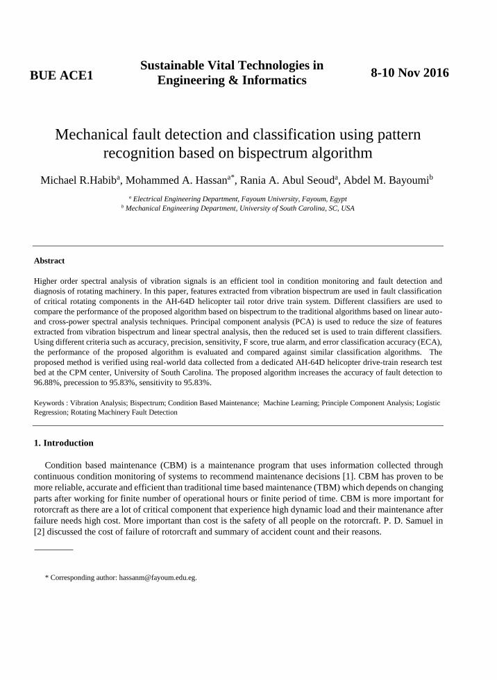
5.2. PCA feature selection

PCA algorithm is used to reduce the number of features extracted from power spectra from 4096 to 95

features. The number of principal components is less than or equal to the number of original samples [11] [13].

Therefore, PCA converts 4096 features to a number of features less than the number of samples which in our

case 96 samples so we get 95 linearly uncorrelated features and every principle component contain some

information as shown in figure 5 which gives loss of information at every principle component we use all the

features given from PCA so as to represent 100% of data information.

Fig. 5. PCA loss of information at every column of PCA features extracted from vibration power spectrum

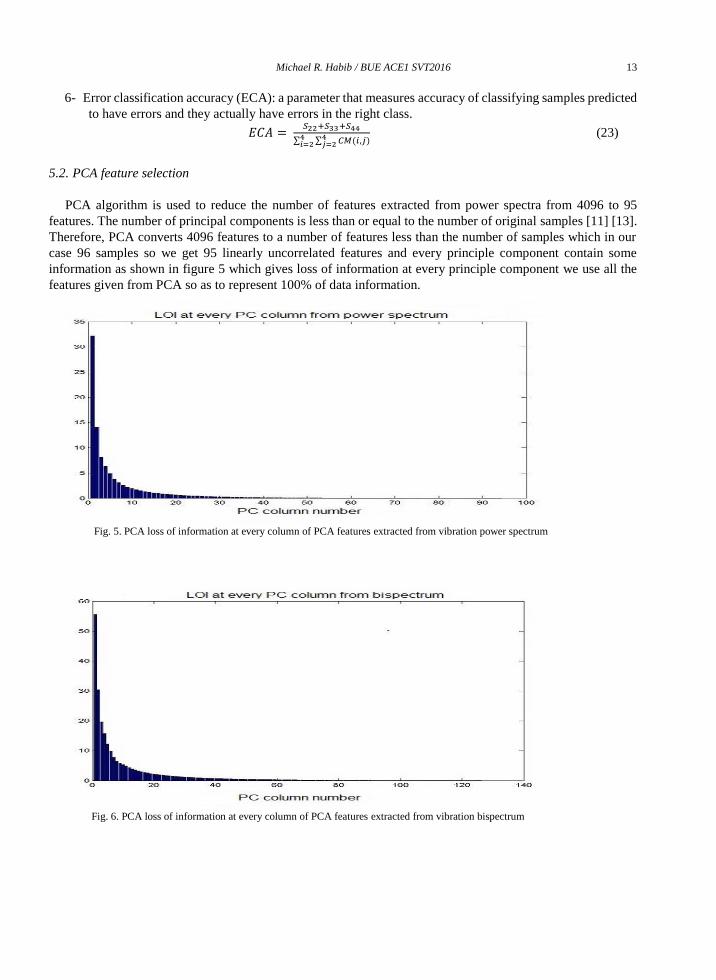
Fig. 6. PCA loss of information at every column of PCA features extracted from vibration bispectrum


Bispectrum has 360000 features which represents a burden on the pattern recognition algorithm. Therefore,

PCA is used to reduce the number of features to a number less than or equal the samples which in this case is

equal to 128 samples. PCA output in this case is 127 linearly uncorrelated features. In PCA, smaller

eigenvalues of covariance matrix provide less pattern information [11]. Figure 6 shows the loss of information

at every principle component of 127 components of the bispectrum. In this paper all the 127 features used in

order not to lose any information.

6. Results

In this section, the results of training different classifiers using features extracted from both bispectrum and

power spectrum are presented and compared using the evaluation criteria discussed above.

For pattern recognition based on feature extracted from power spectrum, the best classification performance

is achieved when logistic regression and neural network are used. Figure 6 and table 1 show the results of

evaluation for all classifiers.

Fig. 7.Comparison of six pattern classifiers using features from power spectrum

Table 1. Comparison of different classifiers using features extracted from power spectrum

Pattern algorithms Accuracy Precision sensitivity F score True alarm ECA

Naïve bayes 93.750 91.89 94.44 93.15 97.29 94.44

Linear discrimint 90.62 92.85 90.27 91.54 97.14 95.58

Quadratic discrimint 91.67 94.20 90.28 92.20 98.55 95.59

Support vector machine 80.21 75.64 81.94 78.66 92.3 81.94

Logistic regression 94.79 93.15 94.44 93.79 98.63 94.44

Neural network 94.79 93.06 93.06 93.06 100 93.05


As indicated in Figure 6 and table 1, the best accuracy is achieved using neural network and logistic

regression and it is equal to 94.79 %. However, for precision and error classification accuracy, quadratic

discrimint analysis gives best results, for sensitivity and F score, logistic regression shows better results than

other and true alarm of the neural network has the best result of 100%. So, in summary, logistic regression

shows best classification performance if power spectrum features are used.

Although bispectrum is more complex techniques than power spectrum and it has more features, using

bispectrum features to train pattern recognition classifiers gives better results. Among different classifiers,

logistic regression and neural network have the best accuracy, precision, sensitivity and ECA. Both of them

also have 100% true alarm. Figure 7 and table 2 compare all classifiers using bispectrum features.

Fig. 8.Comparison of six pattern classifiers using features from bispectrum

Table 2. Comparison of different classifiers using features extracted from bispectrum

Pattern algorithms Accuracy Precision sensitivity F score True alarm ECA

Naïve bayes 81.25 77.32 78.13 77.72 96.91 79.79

Linear discrimint 89.84 92.31 87.50 89.84 98.90 93.33

Quadratic discrimint 88.28 90.11 85.42 87.70 98.90 91.11

Support vector machine 80.47 75.96 82.29 79 92.31 82.29

Logistic regression 96.88 95.83 95.83 95.83 100 95.83

Neural network 96.09 95.79 94.09 95.29 100 95.79

7. conclusion

In this paper, fault detection and diagnosis of a rotating mechanical system have been improved by training a

pattern recognition algorithm using features extracted from vibration bispectra. The proposed algorithm uses

features extracted from both auto- and cross- bispectrum then reduce the feature set using principle component

analysis (PCA). The proposed algorithm has shown the ability to detect 3 different mechanical faults (drive


shaft imbalance, misalignment, and combined case of shaft imbalance and misalignment) and distinguish them

from the healthy case and from each other. Six pattern recognition algorithms have been used to classify the

data collected in this study from trail rotor drive train of an AH64D helicopter. A complete set of criteria has

been used to evaluate the proposed algorithm including accuracy, precision, sensitivity and error classification

accuracy (ECA). The proposed method has shown high performance in all of these criteria. Using features

extracted from the conventional power spectrum, multiclass logistic regression and neural network have shown

the highest classification performance with 94.79% accuracy, 93.15% precision, 94.44% sensitivity, and

94.44% ECA. When feature extracted from bispectrum is used, classification performance has recorded

measurable increase such as 96.88% accuracy, 95.83% precision, 95.83% sensitivity, 100% true alarm and

95.83% ECA. The tradeoff of the proposed technique is its higher complexity and computational cost than

linear power spectrum.

Acknowledgements

This research is funded by the South Carolina Army National Guard and United States Army Aviation and Missile Command via the Center of Predictive Maintenance (CPM) at the University of South Carolina- Columbia USA.

References

[1] Jardine, A. K., Lin, D., & Banjevic, D., 2006. “A review on machinery diagnostics and prognostics implementing condition-based

maintenance” Mechanical Systems and Signal Processing, 20(7), 1483-1510. [2] Samuel, P. D., & Pines, D. J., 2005. “A review of vibration-based techniques for helicopter transmission diagnostics” Journal of Sound

and Vibration, 282(1-2), 475-508. [3] Kang, P., & Birtwhistle, D., 1998. “Analysis of vibration signals for condition monitoring of power switching equipment using wavelet

transform,” in Proc IEEE-SP Int. Symp. Time Frequency and Time Scale Analysis, pp. 6–9.

[4] Baydar, N., & Ball, A., 2003. “Detection of gear failures via vibration and acoustic signals using wavelet transform,” Mechanical

Systems and Signal Processing, 17(4), 787-804.

[5] Grabill, P., Seale, J., & Brotherton, T., 2002. “ATEDS: Airborne turbine engine diagnostic system,” 2004 IEEE Aerospace Conference Proceedings (IEEE Cat. No.04TH8720).

[6] Hassan, M. A., Tarbutton, J., Bayoumi, A., & Shin, Y, 2014. “Condition monitoring of helicopter drive shafts using quadratic-

nonlinearity metric based on cross-bispectrum,” IEEE Transactions on Aerospace and Electronic Systems, 50(4), 2819-2829. [7] Rivera, I., Ramirez, A., & Rodriguez, D, 2005. “A time-frequency signal analysis system for power quality assessment,” 48th Midwest

Symposium on Circuits and Systems, 2005., 2, 1670-1680. [8] Hassan, M. A., Bayoumi, A. E., & Shin, Y, 2014. “Quadratic-nonlinearity index based on bicoherence and its application in condition

monitoring of drive-train components,” IEEE Transactions on Instrumentation and Measurement, 63(3), 719-728.

[9] Proakis, J. G., and Manolakis, D. G, 2007. “Power spectrum estimation,” in Digital Signal Proccessing: Principles, Algorithms, and Applications, 4th ed. New Jersey: Prentice Hall, pp. 960-1040.

[10] Kim, Y. C., & Powers, E. J., 1979. “Digital bispectral analysis and its applications to nonlinear wave interactions,” IEEE Trans. Plasma

Sci. IEEE Transactions on Plasma Science, 7(2), 120-131. [11] Bishop, Christopher M.,2006 “Pattern recognition and machine learning”. New York: Springer.

[12] Ghaderi, A., Mohammadpour, H. A., Ginn, H., & Shin, Y, 2015. “High impedance fault detection in distribution network using time-

frequency based algorithm,” 2015 IEEE Power & Energy Society General Meeting.

[13] Hotelling, H., 1933.” Analysis of a complex of statistical variables into principal components,” Baltimore: Warwick & York.

Mechanical fault detection and classification using ... · Mechanical fault detection and...

Documents

Transcript of Mechanical fault detection and classification using ... · Mechanical fault detection and...