MECH370: Modelling, Simulation and Analysis of...

MECH370: Modelling, Simulation and Analysis of

Physical SystemsChapter 2

Modeling of Translational Mechanical SystemElements and element laws of translational mechanical systemsFree body diagram (FBD)Interconnection lawsObtaining the system model

Lecture Notes on Lecture Notes on MECH 370MECH 370 –– ModellingModelling, Simulation and Analysis of Physical Systems, Youmin Zhang (CU), Simulation and Analysis of Physical Systems, Youmin Zhang (CU)

Lecture Notes on Lecture Notes on MECH 370MECH 370 –– ModellingModelling, Simulation and Analysis of Physical Systems, Simulation and Analysis of Physical SystemsChapter 2Chapter 2 2

Course OutlineCourse OutlineModellingModelling (Ch. 2,3,4,5,6,9,10,11,12) Simulation (4) Analysis (7(Ch. 2,3,4,5,6,9,10,11,12) Simulation (4) Analysis (7,8),8)

1. Definition and classification of dynamic systems (chapter 1)

2. Translational mechanical systems (chapter 2)3. Standard forms for system models (chapter 3)4. Block diagrams and computer simulation with

Matlab/Simulink (chapter 4)5. Rotational mechanical systems (chapter 5)6. Electrical systems (chapter 6)7. Analysis and solution techniques for linear systems

(chapters 7 and 8)8. Developing a linear model (chapter 9)9. Electromechanical systems (chapter 10)10.Thermal and fluid systems (chapters 11, 12)


Why Mathematical Models are Needed? Why Mathematical Models are Needed? ReviewReview

• Analogous SystemsCan have the same mathematical model for

different types of physical systemsCommon analysis methods and tools can be used


Procedure of System ModelingProcedure of System ModelingReviewReview

• Divide the system into idealized components• Apply physical laws to the elements• Apply interconnection laws between elements• Combine the equations to obtain the model


Overview of Element Models in Physical SystemsOverview of Element Models in Physical SystemsMechanical Translational ModelsMechanical Translational Models

MM

xx

ffxx

BB

ff

ff xx

kk

force/velocity force/position

Mass f = M dv/dt f = M dx2 /dt2

Damper(Viscous friction)

f = B v f = B dx/dt

Spring(Stiffness)

f = k ∫ v dt f = k x


torque/velocity torque/position

Inertia T = J dω/dt T = J dθ2/dt2

Viscous friction

T = B ω T = B dθ/dt

Stiffness T = s ∫ ω dt T = s θ

T, T, θθ

JJ

BB

T, T, θθ

T, T, θθ

ss

Overview of Element Models in Physical SystemsOverview of Element Models in Physical SystemsMechanical Rotational ModelsMechanical Rotational Models


voltage/current voltage/charge

Inductance v = L di/dt v = L dq2/dt2

Resistance v = R i v = R dq/dt

Capacitance v = 1/C ∫ i dt v = 1/C q

ii++vv__

ii++vv__

ii ++vv__

Overview of Element Models in Physical SystemsOverview of Element Models in Physical SystemsElectrical Component ModelsElectrical Component Models


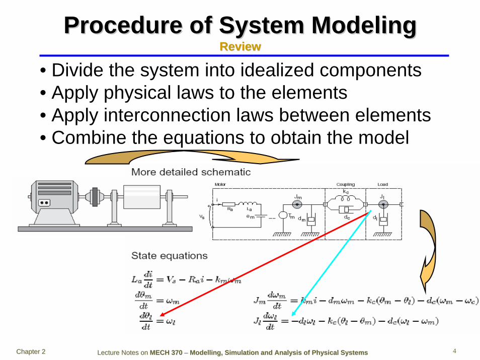
Transformer

Lever

Gears

ii11

vv11

ii22

vv22

NN22NN11

TT1 1 , , θθ11

TT2 2 , , θθ22

NN11

NN22

ff11 , x, x11

ff22 , x, x22

LL11

LL22

v1 N1=

v2 N2

i1 N2=

i2 N1

f1 L2=

f2 L1

x1 L1=

x2 L2

T1 N1=

T2 N2

θ1 N2=

θ2 N1

Overview of Element Models in Physical SystemsOverview of Element Models in Physical SystemsTransformation ModelsTransformation Models


Mathematical Mathematical ModellingModelling of of Mechanical SystemsMechanical Systems

Elementary parts• A means for storing kinetic energy (mass or inertia)

• A means for storing potential energy (spring or elasticity)

• A means by which energy is gradually dissipated (damper)


Mathematical Mathematical ModellingModelling of of Mechanical SystemsMechanical Systems

Motion in mechanical systems can be• Translational• Rotational, or• Combination of aboveMechanical systems can be of two types• Translational systems• Rotational systemsVariables that describe motion• Displacement, x• Velocity, v• Acceleration, a


Modeling of translational mechanical systems Modeling of translational mechanical systems VariablesVariables

xdtdxv == &

xxdtd

dtd

dtdva &&=== )(

dtdWxfvfP =⋅=⋅= &

• x: displacement (m)

• v: velocity (m/sec)

• a: acceleration (m/sec )

• f: force (N)

• P: power (Nm/sec, Watt)

• W: work (energy) (Nm, J)All these variables are functions of time, t.Power is defined to be the rate at which energy is supplied or dissipated.

2

MM

xx

ffxx

BB

ff

ff xx

kk∫+= 1

001

t

tdt)t(P)t(W)t(W


∫1

0

t

tdt)t(P

∫+= 1

001

t

tdt)t(P)t(W)t(W

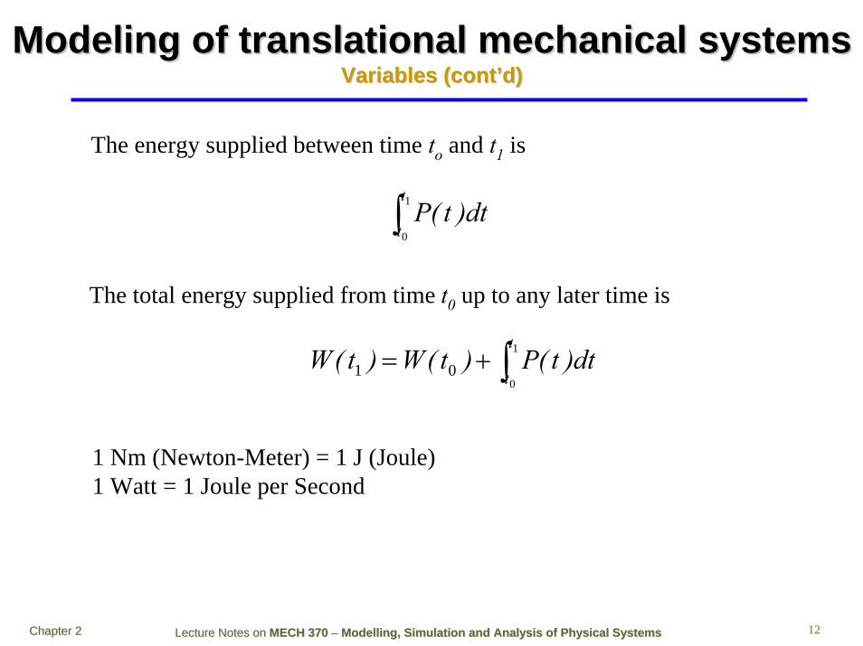
The energy supplied between time to and t1 is

The total energy supplied from time t0 up to any later time is

1 Nm (Newton-Meter) = 1 J (Joule)1 Watt = 1 Joule per Second

Modeling of translational mechanical systems Modeling of translational mechanical systems Variables (contVariables (cont’’d)d)


Modeling of translational mechanical systems Modeling of translational mechanical systems ElementsElements

• Three primary elements of interest– Mass (inertia) m (or M)– Stiffness (spring) k– Friction - Dissipation (damper) B– Usually we deal with “equivalent” m, B, k

Distributed mass -> lumped mass• Lumped parameters– Mass maintains motion– Stiffness restores motion– Damping eliminates motion

mm

xx

ffxx

BB

ff

ff xx

kk


ElementsElements

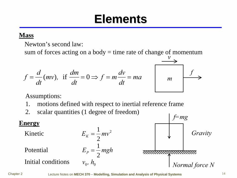
Newton’s second law: sum of forces acting on a body = time rate of change of momentum

madtdvmf

dtdm,mv

dtdf ==⇒== 0 if )(

Assumptions:1. motions defined with respect to inertial reference frame2. scalar quantities (1 degree of freedom)

m

v

f

Energy

Mass

2

21 mvEK =

mghEP 21

=

00, hv

Potential

Initial conditions

Kinetic

Normal force N

f=mg

Gravity


Elements (contElements (cont’’d)d)

Stiffness is the resistance of an elastic body to deflection or deformationby an applied force

Stiffness (N/m)

Most common: ideal spring

d0+x

x

kxfdtdtxtxdtd

fxd

=−=⇒+=

==

00

0

)( )( )()(by caused elongation

applied is force no when spring oflength

k: stiffness constant


Elements (contElements (cont’’d)d)

Multiple applied forces: xk)xx(kf Δ=−= 12

The linear spring is an approximation of something likef

x

k

x1 x2

kff

Linear

Non-linear

f

x


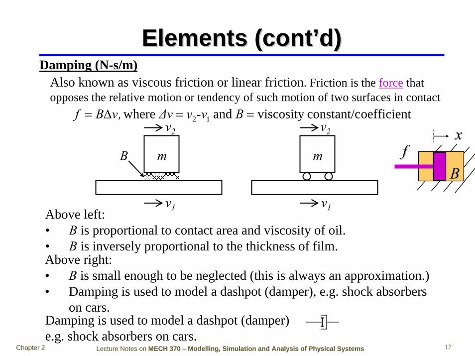
Elements (contElements (cont’’d)d)Also known as viscous friction or linear friction. Friction is the force that opposes the relative motion or tendency of such motion of two surfaces in contact

Damping (N-s/m)

oefficientconstant/cviscosity and where 12 ==Δ= B-vvΔv,vBf

Above left: • B is proportional to contact area and viscosity of oil.• B is inversely proportional to the thickness of film.Above right:• B is small enough to be neglected (this is always an approximation.)• Damping is used to model a dashpot (damper), e.g. shock absorbers

on cars.Damping is used to model a dashpot (damper)e.g. shock absorbers on cars.

B

v2

v1

m

v1

m

v2

ffxx

BB

http://en.wikipedia.org/wiki/Force


Element Laws

ifdtdvm

dtxdmma ∑=== 2

2

)xx(kf 12 −=

vB)vv(Bf Δ=−= 12Friction(Damping):

Mass: Newton’s 2nd Law

Stiffness(Spring):

mfi

x

x1 x2

kff

Bv2

v1

m

v1

m

v2

v2f

x1 x2

ffB No friction

Idealized shock absorber (dashpot)

B: viscosity constant, unit: N-s/m


Element Laws (cont’d)

vBf Δ=

)v(Asignf Δ=

axCf Δ=

Viscous friction: f

Δv

k

Coulomb (dry) friction:

Drag:

fA

Δv-A

f

Δv


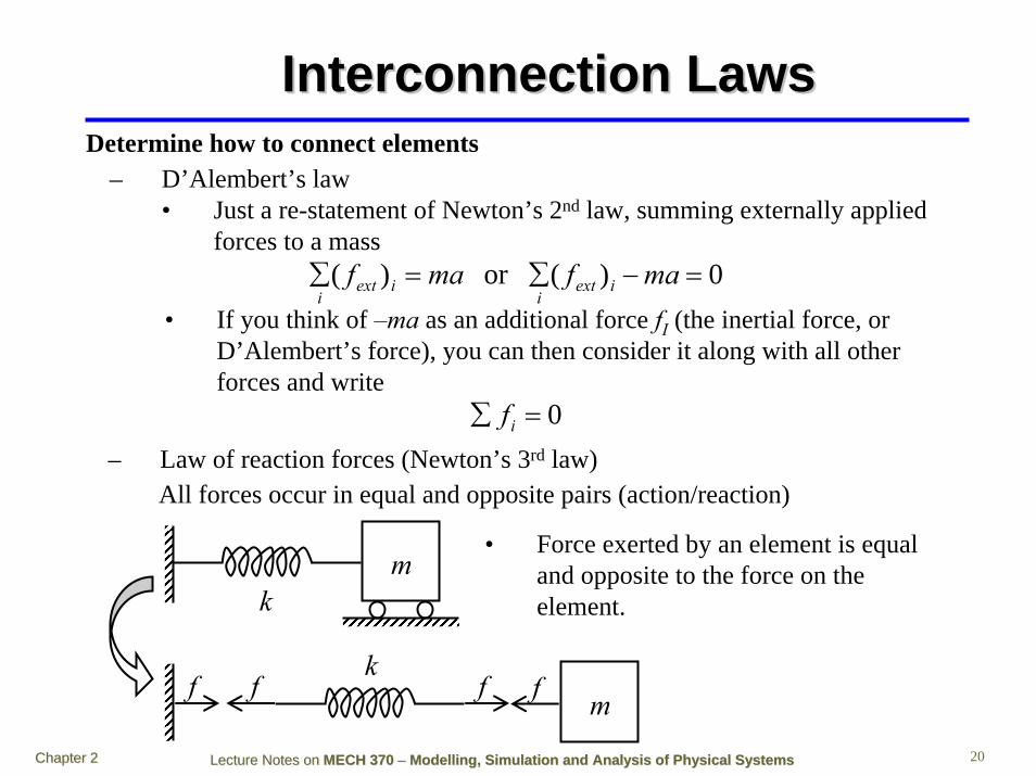
Interconnection LawsInterconnection Laws

– D’Alembert’s law• Just a re-statement of Newton’s 2nd law, summing externally applied

forces to a mass0)(or )( =−∑=∑ mafmaf iext

iiext

i• If you think of –ma as an additional force fI (the inertial force, or

D’Alembert’s force), you can then consider it along with all other forces and write

0=∑ if

All forces occur in equal and opposite pairs (action/reaction)

Determine how to connect elements

– Law of reaction forces (Newton’s 3rd law)

km

mfffk

f

• Force exerted by an element is equal and opposite to the force on the element.


Law of Displacements– If the ends of two elements are connected, these ends are forced to

move with the same displacement, velocity, and acceleration.

00

mass no

=∑⇒∑=/⇑

iiP

P ffdt

dvm 0211 =+−− kBk fff

– Newton’s 2nd law at a point:The sum of the forces at a connection between elements equals zero.

xv

mxv

xv

km

x

vB

k1 k2

x1v1

x1v1

k2

x1v1

k1

f1 f2

fn

k1

B1

k2fk1

fB1

fk2

x

y


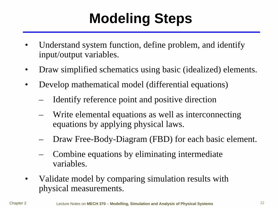
Modeling Steps

• Understand system function, define problem, and identify input/output variables.

• Draw simplified schematics using basic (idealized) elements.

• Develop mathematical model (differential equations)

– Identify reference point and positive direction

– Write elemental equations as well as interconnecting equations by applying physical laws.

– Draw Free-Body-Diagram (FBD) for each basic element.

– Combine equations by eliminating intermediate variables.

• Validate model by comparing simulation results with physical measurements.


Obtaining the System ModelExample: a mass-spring-damper system

)t(fkxxBxm

)t(fkxdtdxB

dtxdm

vdtdx),t(fkxBv

dtdvm

kxBv)t(fff)t(fdtdvm

a

a

a

akBa

=++

=++

==++

−−=−−=

&&&

2

2

Free Body Diagram (FBD):

Newton’s 2nd Law:

km fa(t)

B x, v

m

fB

fk

fa(t)

fI

Force exerted by the dashpot

the applied force

Force exerted by the spring

the initial force

x

y


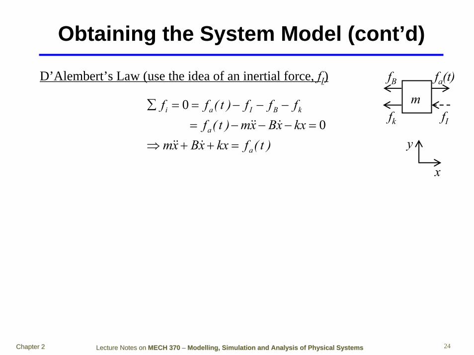
Obtaining the System Model (cont’d)

D’Alembert’s Law (use the idea of an inertial force, fI)

)t(fkxxBxmkxxBxm)t(ffff)t(ff

a

a

kBIai

=++⇒=−−−=

−−−==∑

&&&

&&& 0 0 m

fB

fk

fa(t)

fI

x

y



• EOM of the above simple mass-spring-damper system

ForceApplied TotalSpring theof

nContribuioDamper theof

ContribtinInertia of

Contibutin)t(fkxxBxm a=++ &&&

We now want to look at the energy distribution of the system. How should we do it?

43421&&&&&&&

Power

x)t(fxkxxxBxxm a ⋅=⋅+⋅+⋅

• Integrate the 2nd equation w.r.t. (with respect to) time:

43421&

43421&

43421&&

43421&&&

&

10

1

0

1

0

10

2

1

0

1

0

to timefrom force applied the

by done work Totalenergy potential

of Changedamperby dissipatedEnergy

0

energykenetic of change

tt(t)f

W

t

t a

E

t

t

dtxB

t

t

E

t

t

a

Pttk

dtx)t(fdtxkxdtxxBdtxxm ∫∫∫∫ ⋅=⋅+⋅+⋅

Δ∫ ≥Δ

Energy distribution:

• Multiply the above equation by the velocity v: (since P is defined as P=fv)


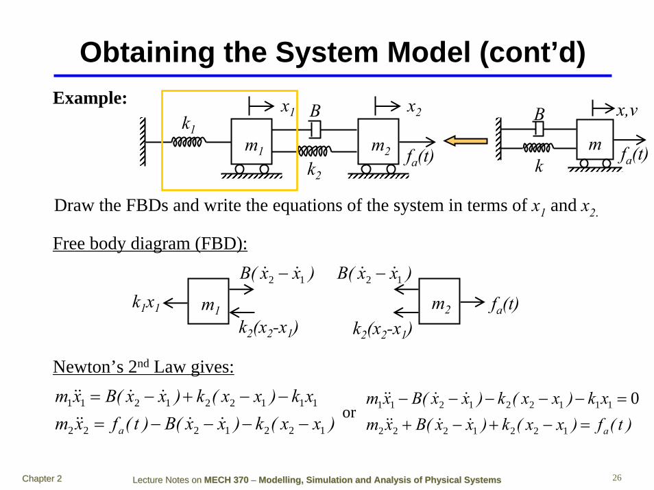
Obtaining the System Model (cont’d)Example:

Free body diagram (FBD):

Draw the FBDs and write the equations of the system in terms of x1 and x2.

)xx(k)xx(B)t(fxmxk)xx(k)xx(Bxm

a 1221222

111221211

−−−−=−−+−=

&&&&

&&&&

Newton’s 2nd Law gives:

m2 fa(t)

B x2

m1

k1

k2

x1

k1x1

k2(x2-x1)m1

)xx(B 12 && −

fa(t)m2

k2(x2-x1)

)xx(B 12 && −

km fa(t)

B x,v

)t(f)xx(k)xx(Bxmxk)xx(k)xx(Bxm

a=−+−+=−−−−−

1221222

111221211 0&&&&

&&&&or


Obtaining the System Model (contObtaining the System Model (cont’’d)d)How about deriving the equations using D’Alembert’s Law?


k1x1

k2(x2-x1)m1

)xx(B 12 && − fa(t)m2

k2(x2-x1)

)xx(B 12 && −

11xm && 22xm &&

00

2212212

111112212

=−−−−−=−−−+−xm)xx(k)xx(B)t(f

xmxk)xx(k)xx(B

a &&&&

&&&&

or

)t(f)xx(k)xx(Bxmxk)xx(k)xx(Bxm

a=−+−+=−−−−−

1221222

111221211 0&&&&

&&&&

k1x1

k2(x2-x1)m1

)xx(B 12 && −

fa(t)m2

k2(x2-x1)

)xx(B 12 && −


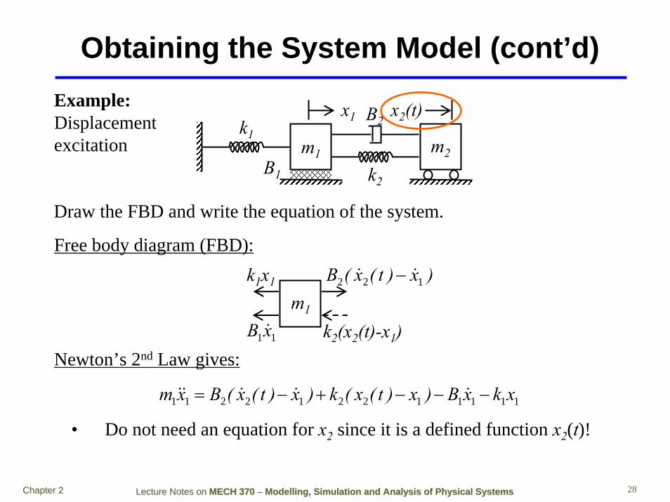
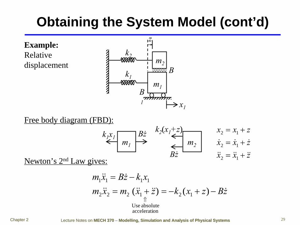
Obtaining the System Model (cont’d)Example:Displacementexcitation


Draw the FBD and write the equation of the system.


m2

B2x2(t)

m1

k1

k2

x1

B1

k1x1

k2(x2(t)-x1)m1

)x)t(x(B 122 && −

11xB &

111112212211 xkxB)x)t(x(k)x)t(x(Bxm −−−+−= &&&&&

• Do not need an equation for x2 since it is a defined function x2(t)!



zxxzxxzxx

&&&&&&

&&&

+=+=+=

12

12

12

zBzxkzxmxmxkzBxm

&&&&&&&

&&&

−+−=+=−=

⇑)()( 12

onacceleratiabsolute Use

1222

1111

Example:Relativedisplacement



m2

m1

x1

k1

B1

k2

z

B

k1x1m1

zB&m2

zB&

k2(x1+z)


Ideal Pulley ElementIdeal Pulley Element

m1

m2

T

T

• No mass, no friction, no slippage between cable and cylinder.

• Cable is always in tension.

• Cable cannot stretch.

If the pulley is not ideal, its mass and any frictional effects must be considered.

Assumption for ideal pulley:


Ideal Pulley Element (contIdeal Pulley Element (cont’’d)d)

)t(f)xx(kxBxmxB)xx(k)t(fxm

a

a

=−++∴+−+−=−

2111111

1121111

:M1

&&&

&&&

)xx(kgmxkxBxmgmxBxk)xx(kxm

2112222222

2222221122

:M2

−=+++∴−−−−=

&&&

&&&

Example:


Find the equation describing the system with pulley.

Equations:

m2

T

m1fa(t)B1

x1

k1

B2k2

x2k1 (x1-x2)

m1xB &1

fa(t)m2

k1 (x1-x2)

m2 gk2 x2

something new here!

xB &2


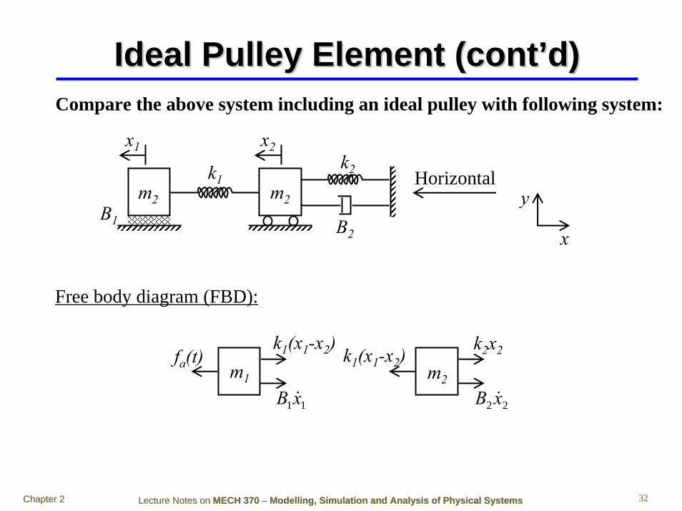
Ideal Pulley Element (contIdeal Pulley Element (cont’’d)d)Compare the above system including an ideal pulley with following system:

fa(t)k1(x1-x2)

m1

11xB &

k2x2

m2

22 xB &

k1(x1-x2)

m2

B2

m2

k1k2

x1

B1

x2

Horizontal

x

y



Ideal Pulley Element (contIdeal Pulley Element (cont’’d)d)

)xx(kxkxBxmxBxk)xx(kxm

)t(f)xx(kvBvm)t(f)xx(kxBxmxB)xx(k)t(fxm

a

a

a

211222222

222221122

2111111

2111111

1121111

:M2

or

:M1

−=++∴−−−=

=−++=−++∴

+−+−=−

&&&

&&&

&

&&&

&&&

p.32 )28( 211222222

2111111

22

,)xx(kxkxBxm)t(f)xx(kvBvm

vv

a

⎪⎭

⎪⎬⎫

−=++=−++

⇑⇑&&&

&

&

Equations for the system:

Finally,

m

x

fa(t)

m

x

fa(t)

)t(fxm a=&&

)t(fxm)t(fxm

a

a

=∴−=−

&&

&& x

y

)t(f)xx(kxBxm a=−++ 2111111 :M1 &&&

)xx(kgmxkxBxm 2112222222 :M2 −=+++ &&&


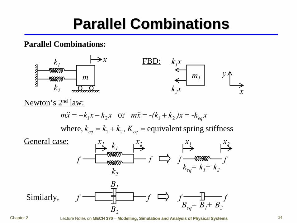
Parallel CombinationsParallel Combinations

stiffness spring equivalent where,

or

21

2121

=+=

=+=−−=

eqeq

eq

K,kkk

x-k)xk-(kxmxkxkxm &&&&

m

xk1

k2 x

yk1x

m1

k2x

Parallel Combinations:

FBD:

Newton’s 2nd law:

General case:

f

k1

k2

f

x1 x2

keq= k1+ k2

f f

x1 x2

fB1

B2

f f fBeq= B1+ B2

Similarly,


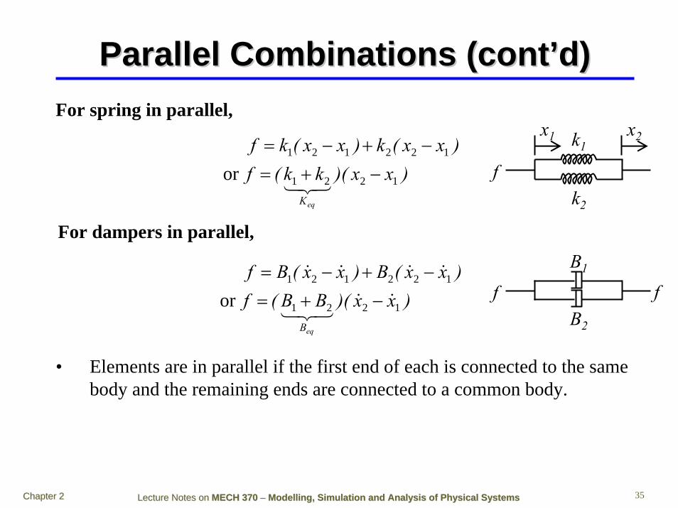
Parallel Combinations (contParallel Combinations (cont’’d)d)For spring in parallel,

)xx)(kk(f)xx(k)xx(kf

eqK

1221

122121

or

−+=−+−=

321

For dampers in parallel,

)xx)(BB(f)xx(B)xx(Bf

eqB

1221

122121

or

&&321

&&&&

−+=−+−=

• Elements are in parallel if the first end of each is connected to the same body and the remaining ends are connected to a common body.

k1

k2

f

x1 x2

fB1

B2

f


Example:

Equivalent system:

B3

m

k2x

B2B1

k1

m

Beq

keq k1x

m xB &3

xB &2

xB &1

k2xfa(t)

xm &&

FBD:

21eq321

21321

21321

where,

then,

kkk,BBBB

)t(fxkxBxm

x)kk(x)BBB()t(fxkxkxBxBxB)t(fxm

eq

aeqeq

kB

a

a

eqeq

+=++=

=++

+−++−=−−−−−=

&&&

321&

43421

&&&&&

Equations:

x

y

Parallel Combinations (contParallel Combinations (cont’’d)d)


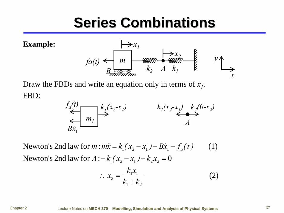
Series CombinationsSeries CombinationsExample:

Draw the FBDs and write an equation only in terms of x1.

mk2

x1

Bfa(t)

k1A

x2

x

y

FBD:fa(t)

m1

1xB&

k1(x2-x1)

A

k2(0-x2)k1(x2-x1)

(2)

0 :for law 2nd sNewton'(1) :for law 2nd sNewton'

21

112

22121

1121

kkxkx

xk)xx(kA)t(fxB)xx(kxmm a

+=∴

=−−−−−−= &&&


Series Combinations (contSeries Combinations (cont’’d)d)Substitute (2) into (1) to get:

21

21

21eq

1121

21

121

121

21

111

111k where,

kkkk

kk

)t(fxBxkk

kkxm

)t(fxB)kk

x)kk(kk

xk(kxm

a

k

a

eq

+=

+=

−−+

−=

−−++

−+

=

&

43421

&&

&&&


SummarySummary• Understand the system and identify the elements and variables.

• Divide system into idealized elements: mass, stiffness, friction, pulley.

• Find the element laws:

• Use the interconnection laws:

vBfx,kf,fxm i Δ=Δ=∑= &&

• Apply Newton’s 2nd law to masses, nodes with unknown v and use element, interconnection laws to determine forces in terms of x, v.

f f

Newton’s 3rd law

x

Law of displacement

x

Newton’s 2nd law

fi0=∑ if


Reading and ExerciseReading and Exercise• Reading

Chapter 2

• Assignment #1Ex: 2.1, 2.2, 2.16, 2.22, 3.13, 3.28 (to be

handed in for marking)

Due: Fri., 6/7/07 at lecture

Ex: 2.10, 2.27, 3.1, 3.15, 3.18 (for your practice, no need to hand in)

MECH370: Modelling, Simulation and Analysis of...

Documents

Transcript of MECH370: Modelling, Simulation and Analysis of...