MECH 401 Mechanical Design ApplicationsDr. M. O’Malley– Master Notes

Spring 2006Dr. D. M. McStravickRice University

ReadingChapter 7

HomeworkHW #4 available, due 2-14

TestsQuiz #2 will be in class on 2-16

Nature of fatigue failure

Starts with a crack Usually at a stress concentration

Crack propagates until the material fractures suddenlyFatigue failure is typically sudden and complete, and doesn’t give warning

Fatigue Failure Examples

Door Stop [Text fig 6-12]Rocker Arm [Text fig. 6-9]Auto Door Handle [Text fig. 6-7]Large Flanged Connection FailureJacob Neu chair failure

Fatigue

Fatigue strength and endurance limitEstimating FS and ELModifying factors

Thus far we’ve studied static failure of machine elementsThe second major class of component failure is due to dynamic loading

Variable stressesRepeated stressesAlternating stressesFluctuating stresses

The ultimate strength of a material (Su) is the maximum stress a material can sustain before failure assuming the load is applied only once and heldA material can also fail by being loaded repeatedly to a stress level that is LESS than Su

Fatigue failure

More Fatigue Failure Examples (ASM)

More Fatigue Failure Examples (ASM)

Approach to fatigue failure in analysis and design

Fatigue-life methods (7-3 to 7-6)Stress-life method (rest of chapter 7)

Fatigue-life methods

Three major methodsStress-lifeStrain-lifeLinear-elastic fracture mechanics

Each predict life in number of cycles to failure, N, for a specified level of loadingLow-cycle fatigue

1≤N≤103 cyclesHigh-cycle fatigue

N>103 cycles

The 3 major methods

Stress-lifeBased on stress levels onlyLeast accurate for low-cycle fatigueMost traditional

Easiest to implementAmple supporting dataRepresents high-cycle applications adequately

Strain-lifeMore detailed analysis of plastic deformation at localized regionsGood for low-cycle fatigue applicationsSome uncertainties exist in the results

Linear-elastic fracture mechanicsAssumes crack is already present and detectedPredicts crack growth with respect to stress intensityPractical when applied to large structures in conjunction with computer codes and periodic inspection

Strain-life method

Fatigue failure almost always begins at local discontinuity

Notch, crack or other SCWhen stress at discontinuity > elastic limit, plastic strain occursFatigue fracture occurs for cyclic plastic strains

Can find fatigue life given strain and other cyclic characteristics

Often the designer does not have these a priori

Linear-elastic fracture mechanics method

Stage 1 – crystal slip through several contiguous grainsStage 2 – crack extensionStage 3 – fractureMethod involves

Determining stress intensity as function of crack lengthFrom here, determine life

In reality, computer programs are used to calculate fatigue crack growth and therefore onset of failure

Fatigue analysis

Always good engineering practice to conduct a testing program on the materials to be employed in design and manufactureIs actually a requirement in guarding against possibility of fatigue failureBecause of this necessity, it would really be unnecessary for usto proceed in study of fatigue failure except for one important reason:

The desire to know why fatigue failures occur so that the most effective method or methods can be used to improve fatigue strength

Stress-life method Least accurate for low-cycleMost traditionalWe will come back to this method later

Fatigue analysis

2 primary classifications of fatigue

Alternating – no DC component

Fluctuating – non-zero DC component

Analysis of alternating stresses

As the number of cycles increases, the fatigue strength Sf (the point of failure due to fatigue loading) decreasesFor steel and titanium, this fatigue strength is never less than the endurance limit, SeOur design criteria is:

As the number of cycles approaches infinity (N ∞), Sf(N) = Se (for iron or Steel)

a

f NSσ

η′

=)(

Method of calculating fatigue strength

Seems like we should be able to use graphs like this to calculate our fatigue strength if we know the material and the number of cyclesWe could use our factor of safety equation as our design equation

But there are a couple of problems with this approach

S-N information is difficult to obtain and thus is much more scarce than σ−ε informationS-N diagram is created for a lab specimen

SmoothCircularIdeal conditions

Therefore, we need analytical methods for estimating Sf(N) and Se

a

f NSσ

η′

=)(

Terminology and notationInfinite life versus finite life

Infinite life Implies N ∞Use endurance limit (Se) of materialLowest value for strength

Finite lifeImplies we know a value of N (number of cycles)Use fatigue strength (Sf) of the material (higher than Se)

Prime (‘) versus no primeVariables with a ‘ (Se’)

Implies that the value of that strength (endurance limit) applies to a LAB SPECIMEN in controlled conditions

Variables without a ‘ (Se, Sf)Implies that the value of that strength applies to an actual case

First we find the prime value for our situation (Se’)Then we will modify this value to account for differences between a lab specimen and our actual situationThis will give us Se (depending on whether we are considering infinite life or finite life)Note that our design equation uses Sf, so we won’t be able to account for safety factors until we have calculated Se’ and Se

a

f NSσ

η′

=)(

Estimating Se’ – Steel and Iron

For steels and irons, we can estimate the endurance limit (Se’) based on the ultimate strength of the material (Sut)

SteelSe’ = 0.504 Sut for Sut < 212 ksi (1460 MPa)

= 107 ksi (740 MPa) for all other values of Sut

IronSe’ = 0.4 Sut for Sut < 60 ksi (400 MPa)

= 24 ksi (160 MPa) for all other values of Sut

S-N Plot with Endurance Limit

Estimating Se’ – Aluminum and Copper Alloys

For aluminum and copper alloys, there is no endurance limitEventually, these materials will fail due to repeated loadingTo come up with an “equivalent” endurance limit, designers typically use the value of the fatigue strength (Sf’) at 108 cycles

Aluminum alloysSe’ (Sf at 108 cycles) = 0.4 Sut for Sut < 48 ksi (330 MPa)

= 19 ksi (130 MPa) for all other values of Sut

Copper alloysSe’ (Sf at 108 cycles) = 0.4 Sut for Sut < 40 ksi (280 MPa)

= 14 ksi (100 MPa) for all other values of Sut

Constructing an estimated S-N diagram

Note that Se’ is going to be our material strength due to “infinite”loading

We can estimate an S-N diagram and see the difference in fatigue strength after repeated loading

For steel and iron, note that the fatigue strength (Sf) is never less than the endurance limit (Se’)

For aluminum and copper, note that the fatigue strength (Sf) eventually goes to zero (failure!), but we will use the value of Sf at 108 cycles as our endurance limit (Se’) for these materials

Estimating the value of Sf

When we are studying a case of fatigue with a known number of cycles (N), we need to calculate the fatigue strength (Sf)We have two S-N diagrams

One for steel and ironOne for aluminum and copper

We will use these diagrams to come up with equations for calculating Sf for a known number of cyclesNote: Book indicates that 0.9 is not actually a constant, and uses the variable f to donate this multiplier. We will in general use 0.9.

Estimating Sf (N)

For steel and iron

For aluminum and copper

( )

( ) ( ) bSaSSb

aNNS

ut

e

ut

bf

39.0loglog

9.0log31

−=

⎟⎟⎠

⎞⎜⎜⎝

⎛′

−=

=

( )

( ) ( ) bSaSSb

aNNS

ut

e

ut

bf

39.0loglog

9.0log7.5

1

−=

⎟⎟⎠

⎞⎜⎜⎝

⎛′

−=

= For N < 108

Where Se’ is the value of Sf at N = 108

For 103 < N < 106

Correction factorsNow we have Se’ (infinite life) We need to account for differences between the lab specimen and a real specimen (material, manufacturing, environment, design)We use correction factors

Strength reduction factorsMarin modification factors

These will account for differences between an ideal lab specimen and real lifeSe = ka kb kc kd ke kf Se’

ka – surface factorkb – size factorkc – load factorkd – temperature factorke – reliability factorKf – miscellaneous-effects factorModification factors have been found empirically and are described in section 7-9 of Shigley-Mischke-Budynas (see examples)

If calculating fatigue strength for finite life, (Sf), use equations on previous slide

Endurance limit modifying factors

Surface (ka)Accounts for different surface finishes

Ground, machined, cold-drawn, hot-rolled, as-forgedSize (kb)

Different factors depending on loadingBending and torsion (see pg. 329)Axial (kb = 1)

Loading (kc)Endurance limits differ with Sut based on fatigue loading (bending, axial, torsion)

Temperature (kd)Accounts for effects of operating temperature

Reliability (ke)Accounts for scatter of data from actual test resultsWe will probably not address ke

Miscellaneous-effects (kf)Accounts for reduction in endurance limit due to all other effectsReminder that these must be accounted for

Residual stressesCorrosionetc

Now what?

Now that we know the strength of our part under non-laboratory conditions…… how do we use it?

Choose a failure criterionPredict failure

Part will fail if:σ’ > Sf(N)Factor of safety:η = Sf(N) / σ’Life of part

b = - 1/3 log (0.9 Sut / Se) log(a) = log (0.9 Sut) - 3b

b

aN

1

⎟⎠⎞

⎜⎝⎛ ′

=σ

Stress concentrations and fatigue failure

Unlike with static loading, both ductile and brittle materials are significantly affected by stress concentrations for repeated loading casesWe use stress concentration factors to modify the nominal stressSC factor is different for ductile and brittle materials

SC factor – fatigue

σ = kfσnom+ = kfσo

τ = kfsτnom = kfsτo

kf is a reduced value of kT and σo is the nominal stress.kf called fatigue stress concentration factorWhy reduced? Some materials are not fully sensitive to the presence of notches (SC’s) therefore, depending on the material, we reduce the effect of the SC

Fatigue SC factor

kf = [1 + q(kt – 1)]kfs = [1 + qshear(kts – 1)]

kt or kts and nominal stressesPages 982-988

q and qshearNotch sensitivity factorFind using figures 7-20 and 7-21 in book (SMB) for steels and aluminumsUse q = 0.20 for cast iron

Brittle materials have low sensitivity to notchesAs kf approaches kt, q increasing (sensitivity to notches, SC’s)If kf ~ 1, insensitive (q = 0)

Property of the material

Example

AISI 1020 as-rolled steelMachined finishFind Fmax for:

η = 1.8Infinite life

Design Equation:η = Se / σ’

Se because infinite life

Example, cont.

η = Se / σ’What do we need?

Se

σ’Considerations?

Infinite life, steelModification factorsStress concentration (hole)

Find σ’nom (without SC)

( ) ( ) FFhdb

PAP

nom 2083101260

=−

=−

==′σ

Example, cont.

Now add SC factor:

From Fig. 7-20,r = 6 mmSut = 448 MPa = 65.0 ksiq ~ 0.8

( )[ ] nomtnomf kqk σσσ ′−+=′=′ 11

Example, cont.

From Fig. A-15-1,Unloaded holed/b = 12/60 = 0.2kt ~ 2.5

q = 0.8kt = 2.5σ’nom = 2083 F

( )[ ]( )[ ] ( )

( )FF

kq nomt

4583208315.28.01

11

=′−+=′

′−+=′

σσ

σσ

Example, cont.

Now, estimate SeSteel:Se’ = 0.504 Sut for Sut < 1400 MPa (eqn. 7-8)

740 MPa elseAISI 1020 As-rolled

Sut = 448 MPaSe’ = 0.506(448) = 227 MPa

Constructing an estimated S-N diagram

Note that Se’ is going to be our material strength due to “infinite”loading

We can estimate an S-N diagram and see the difference in fatigue strength after repeated loading

For steel and iron, note that the fatigue strength (Sf) is never less than the endurance limit (Se’)

For aluminum and copper, note that the fatigue strength (Sf) eventually goes to zero (failure!), but we will use the value of Sf at 108 cycles as our endurance limit (Se’) for these materials

Correction factorsNow we have Se’ (infinite life) We need to account for differences between the lab specimen and a real specimen (material, manufacturing, environment, design)We use correction factors

Strength reduction factorsMarin modification factors

These will account for differences between an ideal lab specimen and real lifeSe = ka kb kc kd ke kf Se’

ka – surface factorkb – size factorkc – load factorkd – temperature factorke – reliability factorKf – miscellaneous-effects factorModification factors have been found empirically and are described in section 7-9 of Shigley-Mischke-Budynas (see examples)

If calculating fatigue strength for finite life, (Sf), use equations on previous slide

Example, cont.

Modification factorsSurface: ka = aSut

b (Eq. 7-18)a and b from Table 7-4Machined

ka = (4.45)(448)-0.265 = 0.88

Example, cont.

Size: kbAxial loadingkb = 1 (Eq. 7-20)

Load: kcAxial loadingkc = 0.85 (Eq. 7-25)

Example, cont.

Temperature: kd = 1 (no info given)

Reliability: ke = 1 (no info given)

Miscellaneous:kf = 1

Endurance limit:Se = kakbkckdkekfSe’ = (0.88)(0.85)(227) = 177 MPa

Design Equation:( )

( ) kN 4.218.14583

10x177

8.14583177

6==

==′

=

F

FMPaSe

ση

Fluctuating Fatigue Failures

More Fatigue Failure Examples

Alternating vs. fluctuatingAlternating Fluctuating

IMrAP

a

m

=

=

σ

σ

Alternating Stresses

σa characterizes alternating stress

Fluctuating stresses

Mean Stress

Stress amplitude

Together, σm and σacharacterize fluctuating stress

2minmax σσσ +

=m

2minmax σσσ −

=a

Alternating vs. Fluctuating

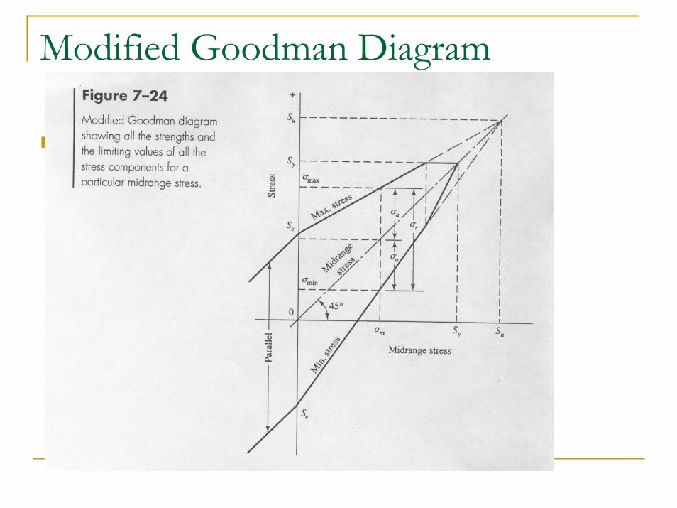
Modified Goodman Diagram

Another Fatigue Failure Representation

Failure criterion for fluctuating loading

SoderbergModified GoodmanGerberASME-ellipticYielding

Points above the line: failureBook uses Goodman primarily

Straight line, therefore easy algebraEasily graphed, every time, for every problemReveals subtleties of insight into fatigue problemsAnswers can be scaled from the diagrams as a check on the algebra

Fluctuating stresses, cont.

As with alternating stresses, fluctuating stresses have been investigated in an empirical mannerFor σm < 0 (compressive mean stress)

σa > Sf FailureSame as with alternating stressesOr,

Static Failure

For σm > 0 (tensile mean stress)Modified Goodman criteria

η < 1 Failure

)S(or max ucycam S≥−= σσσ

ησσ 1

=+ut

m

f

a

SS

Fluctuating stresses, cont.

Relationship is easily seen by plotting:

Goodman LineSafe design region(for arbitrary fluctuationsin σm and σa )

(safe stress line)

1=+ut

m

f

a

SSσσ

ησσ 1

=+ut

m

f

a

SS

Note: σm + σa = σmax

σm + σa > Syt (static failure by yielding)

Important point:Important point: Part can fail because of fluctuations in either σa, σm, or both.Design for prescribed variations in σa and σm to get a more exact solution.

Special cases of fluctuating stresses

Case 1: σm fixed

Case 2: σa fixed

a

aSσ

η =

m

mSσ

η =

Special cases of fluctuating stresses

Case 3: σa / σm fixed

Case 4: both vary arbitrarily

m

m

a

a SSσσ

η ==

ut

m

f

a

SSσσ

η+=

1

Example

Given:Sut = 1400 MPaSyt = 950 MPaHeat-treated (as-forged)Fmean = 9.36 kNFmax = 10.67 kNd/w = 0.133; d/h = 0.55

Find:η for infinite life, assuming Fmean is constant

Example, cont.

Find σm and σa( ) ( )

( )( )

( )( )

MPa28

MPa228

MPa200

Nm 8003.0100.67x141

41

22

Nm 7023.010x36.941

41

22

m 009.02

mx1016.3181075121

121

121

max

maxmaxmax

max

3max

maxmax

3

max

48333

=−=

==

==

===⎟⎠⎞

⎜⎝⎛⎟⎠⎞

⎜⎝⎛=

===⎟⎠⎞

⎜⎝⎛⎟⎠⎞

⎜⎝⎛=

==

=−=−==

=

−

ma

mm

mm

m

IyM

IyM

LFLFM

LFLFM

hy

hdwbhI

IMy

σσσ

σ

σ

σ

Stress Concentration Factor

Example, cont.

Since this is uniaxialloading, σm = 200 MPaσa = 28 MPa

We need to take care of the SC factors

Su = 1400Mpa

kt ~ 2.2 (Figure A15-2)q ~ 0.95 (Table 7-20)kf = 2.14

( )11 −+= tf kqk

nominal

( )( )( )( ) MPa 42820014.2

MPa 602814.2

===′=

===′=

nom

nom

mfmm

afaa

k

k

σσσ

σσσ

Example, cont.

Find strengthEqn. 7-8: S’e = .504Sut

Modification factors

( )

86.0

24.1

808.0

mm 51d2.8 :19)-(7Equation

:Size

107.0

21

eq

=

=

=

≤≤

−

b

eqb

eq

k

dk

hbd

MPa1400S since MPa 700~ ut =′eS

201.0995.0

271

:Surface

=−=

==

a

buta

kba

aSk25)-7 (Eq. 1

Bending:Load

=ck

( )( )( ) MPa12170086.0201.0 ==eS

Example, cont.

Design criteriaGoodman line:

For arbitrary variation in σa and σm,

1=+ut

m

e

a

SSσσ

121

1400

11400121

=+ ma σσ

25.11400428

121601

11400121

=

+=

=+

ηη

ησσ ma

Example, cont.

However, we know that Fmean = constant from problem statement

σm = constant

4.16084

MPa84

11400428

121

1

===

=

=+

=+

a

a

a

a

ut

m

e

a

SS

SSS

S

ση

σ

Less conservative!

Combined loading and fatigueSize factor depends on loadingSC factors also depend on loadingCould be very complicated calculation to keep track of each loadcaseAssuming all stress components are completely reversing and are always in time phase with each other,1. For the strength, use the fully corrected endurance limit for

bending, Se2. Apply the appropriate fatigue SC factors to the torsional stress,

the bending stress, and the axial stress components3. Multiply any alternating axial stress components by the factor

1/kc,ax4. Enter the resultant stresses into a Mohr’s circle analysis to find

the principal stresses5. Using the results of step 4, find the von Mises alternating stress

σa’6. Compare σa’ with Sa to find the factor of safety

Additional details are in Section 7-14