Measuring Transit Timing Variations of Exoplanets using Small

Telescopes

Caroline V. Morley∗

MIT Department of Earth Atmosphere and Planetary Science; MIT Department of Physics

(Dated: May 7, 2010)

Transits of exoplanets were observed from June 2009 through January 2010. Six

transit light curves are presented in this paper for three planets: WASP-10b, WASP-

11/HAT-P-10b, and TrES-3. Measurements of the planetary radii, semi-major axis,

transit duration, and period confirmed literature values to within two sigma. Transit

timing variations were not observed in these systems, but calculations show that it

would be possible to measure transit timing variations induced by large exomoons

(greater than about 6 Earth masses) in the WASP-11/HAT-P-10b system. Chal-

lenges of exoplanet observation from small telescopes are discussed. It was deter-

mined that overall, transit measurements of many exoplanets using small telescopes

can be successful and scientifically useful.

∗cmorley@mit.edu

2

ACKNOWLEDGMENTS

I would like to thank my thesis advisor, Jim Elliot, for all of his help and wisdom during

this project.

I would like to extend a huge thank you to Elisabeth Adams, for everything she taught

me during this process. She guided me through the project, from my first astronomical

observations ever, to data reduction and analysis, to last-minute thesis revisions from her

vacation in Europe. Without all of Elisabeth’s time, effort, and Mathematica code, this

project would never have happened.

I would like to thank Tim Brothers for taking care of all the Wallace telescopes and being

very patient when things occasionally went wrong.

I would like to thank Jane Connor for all of her writing help and support.

I would also like to thank Scott Morrison for observing with me, driving me home from

observation runs, helping me with LaTeX (and grammar), and for generally being patient

and good-humored even when I was not.

3

CONTENTS

Acknowledgments 2

I. Introduction 6

I.1. Scientific Background: Transiting Exoplanets 6

I.2. Earlier Research on Observed Exoplanets 8

I.2.1. WASP-10b 8

I.2.2. TrES-3 10

I.2.3. WASP-11/HAT-P-10b 11

I.3. Goals for Observation of Transits from Wallace Observatory 12

II. Methods for Exoplanet Observation 13

II.1. Preparing to Observe 13

II.2. Observing at Wallace Astrophysical Observatory 14

II.3. Data Reduction 15

II.3.1. Calibration of CCD Frames using IRAF 15

II.3.2. Differential Photometry using IRAF and Mathematica 16

II.4. Transit Fitting 19

II.4.1. Least Squares Fit 19

II.4.2. Calculating Parameters using Least Squares Fit 20

III. Observations 22

III.1. TrES-3 Observations 23

III.2. WASP-10b Observations 25

III.3. WASP-11/HAT-P-10b Observations 27

4

IV. Data Reduction for Observed Transits 29

IV.1. TrES-3 Data Reduction 29

IV.1.1. 2009/06/17 29

IV.1.2. 2009/07/04 29

IV.2. WASP-10b Data Reduction 30

IV.3. WASP-11/HAT-P-10b Data Reduction 30

V. Fitting Light Curves 31

V.1. TrES-3 31

V.2. WASP-10b 32

V.3. WASP-11/HAT-P-10b 32

V.4. Plots 34

VI. Transit Timing Variations (TTV) 37

VI.1. Comparing Measured Transit Midtimes with Literature Midtime Values 37

VI.1.1. TrES-3 TTV 37

VI.1.2. WASP-10b TTV 40

VI.1.3. WASP-11/HAT-P-10b TTV 42

VI.2. Potential for Exomoon detection using Small Telescopes 44

VII. Observing Challenges from Wallace Observatory 49

VII.1. Using Small Telescopes 49

VII.2. Location in Massachusetts 49

VII.3. Examples of “Bad Data” 50

VIII. Conclusions 53

5

VIII.1. Observing Exoplanet Transits and Transit Timing Variations from Small

Telescopes 53

VIII.2. Future Observations 54

IX. Appendix 56

X. Works Cited 57

6

I. INTRODUCTION

I.1. Scientific Background: Transiting Exoplanets

The study of extrasolar planets is a new and dynamic field of research. The first planets

around other stars were discovered in the early 1990s, and as of May 2010, scientists have

discovered 453 exoplanets1. Different methods of detection allow researchers to determine

different planetary parameters. For instance, radial velocity measurements are made using

the doppler shifts in the star’s spectrum from its motion about the center of mass of the

system; these measurements allow scientists to calculate minimum mass of a planet (the

mass multiplied by the sine of the orbital inclination).

Of the known exoplanets, 79 are known to transit — or cross in front of — the central

star1. Using the light curve of a transit, the ratio of the radius of the planet to the radius

of its host star can also be determined. A transiting planet blocks a percentage of light

from the star during the transit; the change in flux from the star during transits observed

to date varies between 2.8% and 0.3%1. A schematic depicting a transiting planet and its

light curve is shown in Figure 1, where the curve shows a small decrease in flux.

By combining the mass, determined using radial velocity calculations, and the radius,

determined from the transit light curve, the density of the planet can be calculated. From

the density, constraints on the planet’s composition can be determined.

Other parameters of the system can also be calculated from the observation of a transit.

Orbital parameters such as period and semi-major axis can be determined by measuring the

shape of a light curve. Also, the shape of the light curve is different in different wavelengths,

a phenomenon caused by a stellar property called limb darkening. Limb darkening refers

1The Extrasolar Planets Encyclopaedia. Web. 02 May 2010. http://exoplanet.eu/

7

FIG. 1. Schematic of Transiting Planet. This image shows an artist’s depiction of a transit.The light curve on the bottom shows how the flux from the star decreases by a small percentagefor the duration of time that the planet blocks the light of a small section of the star. The numberson the image and light curve correspond to moments in time before and during the transit (CentreNational D’etudes Spatiales)

to the fact that because the temperature of the star decreases as a function of increasing

radius within a star, the center of the star’s disk appears to radiate at bluer wavelengths

than the edge of a star. In general, limb darkening effects cause transits measured in red

wavelengths to have light curves with a flatter bottom section than transits measured in

blue wavelengths, because the star is more uniformly bright at redder wavelengths.

Another quantity that can be measured is the midtime of the transit. By comparing

this value to the midtimes of previously measured transits, any variability in the period can

be constrained. These variations, called Transit Timing Variations or TTV, would indicate

the presence of a perturbing body in the system (Holman & Murray, 2005). For instance,

another planet in the system or a large moon around the planet could be detected. Upper

constraints on the mass of such a perturbing object can be made.

The limits of extrasolar planet observation from Wallace Observatory were determined.

8

This determination was challenging because the variability of the weather was a dominating

factor in observations, but some conclusions were drawn about the viability of exoplanet

research at Wallace. In particular, the precision of timing of transits that can be determined

from Wallace data was determined. This is a particularly interesting question because the

telescopes at Wallace Observatory are similar to telescopes generally used by amateur ob-

servers. There are many thousands of amateur telescopes across the country, and I quantified

the precision of transit timing variations (TTV) that they can achieve using this equipment.

Using this value and calculations to determine where viable moons could exist in the sys-

tem, I calculated a lower bound for the mass of a detectable “exomoon” (moon around an

exoplanet) around specific planets in my study. If detections of TTV could be made using

small telescopes, amateurs could play an extremely important role in discovering planets or

moons in known transiting systems.

I.2. Earlier Research on Observed Exoplanets

I.2.1. WASP-10b

WASP-10 (GSC 2752-00114) is a relatively faint star (V = 12.7) located about 90 parsecs

from the Earth (Christian et al. 2009). Stellar parameters for WASP-10 are summarized in

Table I.

TABLE I. Stellar Parameters for WASP-10 from Christian et al. 2009

Parameter Value

RA (J2000) (h min s) 23 15 58.3

Dec. (J2000) (◦ min s) +31 27 46.4

V (Magnitude) 12.7

Distance (parsec) 90 ±20

Teff (K) 4675± 100

9

WASP-10b is a ‘hot Jupiter’ discovered by the Wide Angle Search for Planets (WASP)

Consortium (Christian et al., 2009). This type of planet is called a ‘hot Jupiter’ because it

is similar in mass to Jupiter, but it orbits much closer to the star, making the planet much

hotter than Jupiter. Johnson et al. (2009) suggested that the system had slightly different

planetary parameters than those given by Christian et al. (2009). Johnson et al. included

precision photometry taken using the novel Orthogonal Parallel Transfer Imaging Camera,

mounted on the University of Hawaii 2.2 m telescope atop Mauna Kea, Hawaii. The revised

value for the radius of the planet was 16% smaller than in the previous paper. A summary

of important parameters is shown in Table II.

TABLE II. Literature Values for WASP-10b from Discovery and Follow-up Papers

Parameter Christian et al. 2009 Johnson et al. 2009

Transit Epoch (BJD) 2454357.85808 +0.00041−0.00036 2454664.030913± 0.000082

Orbital Period (days) 3.0927636 +0.0000094−0.000021 3.0927616± 0.0000112

Planet/star area ratio 0.029 +0.001−0.001 0.02525 +0.00024

−0.00028

Planet radius (RJ) 1.28 +0.077−0.091 1.080± 0.020

Transit duration (hours) 2.356344 +0.0456−0.036 2.2271+0.0078

−0.0068

Impact parameter 0.568 +0.054−0.084 0.299 +0.029

−0.043

Planet mass (MJ) 2.96 +0.22−0.17 3.15+0.13

−0.11

Orbital semimajor axis (AU) 0.0369 +0.0012−0.0014 0.03781 +0.00067

−0.00047

10

I.2.2. TrES-3

TrES-3 (GSC 03089-00929) is a 12.4 magnitude G type star. It is located about 400

parsecs from the Solar System (O’Donovan et al., 2007). Stellar parameters for TrES-3 are

summarized in Table III.

TABLE III. Stellar Parameters for TrES-3 from O’Donovan et al., 2007

Parameter Value

RA (J2000) (h min s) 17 52 07.03

Dec. (J2000) (◦ min s) +37 32 46.1

V (Magnitude) 12.402 ± 0.006

Distance (parsec) 400 ± 200

Teff (K) 5720 ± 150

The name TrES-3 also applies to the exoplanet discovered around this star. It was discov-

ered by the Trans-atlantic Exoplanet Survey (TrES) network; O’Donovan et at. announced

the discovery in 2007. TrES-3 is a massive ‘hot Jupiter’ with a very short orbital period

(1.30619 days). TrES-3 is located 0.0226 ± 0.0013 AU from the central star (for reference,

the distance from the Sun to Mercury is about 0.39 AU). A summary of the literature values

of important transit parameters is shown in Table IV.

TABLE IV. Literature Values from TrES-3 Discovery and Follow-up Papers

Parameter O’Donovan 2007 Sozzetti 2008

Transit Epoch (BJD) 2454185.9101 ± 0.0003 2454594.745943 ± 0.000253

Orbital Period (days) 1.30619 ± 0.00001 1.30618581

Planet/star radius ratio 0.1660 ± 0.0024 0.1655±0.0020

Planet radius (RJ) 1.295 ± 0.081 1.336+0.031−0.037

Impact parameter 0.8277 ± 0.0097 0.840 ± 0.010

Planet mass (MJ) 1.92 ± 0.23 1.910+0.075−0.080

Orbital semimajor axis (AU) 0.0226 ± 0.0013 0.02282+0.00023−0.00040

11

I.2.3. WASP-11/HAT-P-10b

WASP-11 or HAT-P-10 (GSC 02340-01714) is an 11.89 magnitude K dwarf star located

125 parsecs away from the Solar System. Stellar parameters for WASP-11/HAT-P-10 are

shown in Table V.

TABLE V. Stellar Parameters for WASP-11/HAT-P-10 from Bakos et al., 2009

Parameter Value

RA (J2000) (h min s) 03 09 29

Dec. (J2000) (◦ min s) +30 40 25

V (Magnitude) 11.89

Distance (parsec) 125 +6−5

Teff (K) 4980 ± 60

WASP-11/HAT-P-10b is a sub-Jupiter sized exoplanet orbiting around WASP-11/HAT-

P-10, discovered by the Wide Angle Search for Planets (WASP) Consortium (Bakos et al.,

2008) and the Hungarian-made Automated Telescope (HAT) Network (West et al., 2008).

The two surveys differ slightly on the precise values of planetary and orbital parameters, but

the planet is approximately 1 Jupiter radius in size and half a Jupiter mass. It orbits the

star in 3.72 days. A summary of the planetary and orbital parameters from both surveys is

included in Table VI.

TABLE VI. Literature Values from WASP-11/HAT-P-10b Discovery Papers

Parameter Bakos et al. (HAT) West et al. (WASP)

Transit Epoch (BJD) 2454185.9101 ± 0.0003 2454473.05586 ± 0.0002

Orbital Period (days) 3.7224690 ± 0.0000067 3.722465+0.000006−0.000008

Planet/star radius ratio 0.1332 ± 0.0013

Planet radius (RJ) 1.045 +0.050−0.033 0.91+0.06

−0.03

Transit duration (days) 0.1100 ± 0.0015 0.1065 0.001−0.0003

Impact parameter 0.238 +0.130−0.093 0.054+0.168

−0.050

Planet mass (MJ) 0.460 ± 0.028 0.53 ± 0.07

Orbital semimajor axis (AU) 0.0439+0.0006−0.0009 0.043 ± 0.002

12

I.3. Goals for Observation of Transits from Wallace Observatory

Using two of the 14-inch telescopes at the George R. Wallace Jr. Astrophysical Obser-

vatory in Westford, MA, transits of the exoplanets presented above were observed. Using

the transit measurements taken, planetary and orbital parameters of each transit light curve

were determined.

For each light curve, the radius of the planet was calculated, and the value from the

literature were compared with this value. The midtime of the transit was also calculated.

By comparing the midtime of the transit with the predicted midtime based on previous

observations, the variability of the period of the orbit was determined. A variable orbital

period would indicate another body in the system, such as a second planet or a large moon.

The duration of the transit was also determined.

The limits of extrasolar planet observation from Wallace Observatory were evaluated.

This evaluation included determining the detectability of transit timing variations, based on

the precision of the transit timing in these light curves.

13

II. METHODS FOR EXOPLANET OBSERVATION

II.1. Preparing to Observe

A transit schedule was created with prediction software written by Elisabeth Adams

(Adams, 2010). The software calculated when transits are observable from WAO by com-

bining the timing of the transit with the altitude of the Sun, proximity and brightness of the

moon, and the airmass of the target in order to determine which transits are visible each

night. The highest airmass allowed was 2.0, the highest altitude of the Sun allowed was -9

degrees, and the closest distance to the moon was 30 degrees.

After determining which transits are visible, finder charts of the fields of view were cre-

ated. These can be created using many different astronomical programs; for this project,

the program Aladin was used to make these finder charts (Bonnarel et al. 2000). Finder

charts were used for determining which transits are measurable from WAO. Specifcally, the

field of view for the target should also include ‘good’ comparison stars, defined as stars of a

comparable magnitude within the field of view. The 14-inch telescopes at WAO have a field

of view of approximately 22 arcminutes, so these comparison stars must be well within that

window to allow for imprecisions in telescope tracking. Also, the target star should be re-

solvable in the image. Most potential target stars are resolvable from the 14-inch telescopes,

which have a plate scale of 1.29 arcseconds/pixel, with the exception of close binary stars

such as HAT-P-1b.

Several possible observing targets were chosen because weather at the observatory pre-

vents observations for much of the time. The process of choosing targets depends on the

following criteria. First, the star must be bright enough for the telescopes to gather enough

photons within about a 3-5 minute exposure time (from WAO telescopes, around V=12

14

is a reasonable brightness). As discussed above, other comparably bright stars should be

within the field of view. Also, the transit should be deep enough to be observable with

the equipment at Wallace; the minimum depth measurable from Wallace was through to be

about 1% due to signal to noise calculations.

II.2. Observing at Wallace Astrophysical Observatory

The telescopes used were two nearly identical Celestron C14 Schmidt-Cassegrain tele-

scopes (referred to in this paper as Pier 3 and Pier 4). These are mounted on equatorial

Paramounts. The CCDs used were SBIG STL-1001E imaging CCD cameras with a 22x22

arcminute field of view and 1.29 arcseconds/pixel. While these telescopes are very similar,

each has slightly different observing properties. For instance, the focus values on Pier 3 and

Pier 4 are not identical, with Pier 3 having slightly better focus.

The R filter is generally used for transit observation, because many stars with transiting

planets emit more light in redder wavelengths than in bluer wavelengths. Another benefit of

the R filter is that there is significantly less background sky light at these wavelengths than

in bluer wavelengths. If, however, the goal for the observation was to observe stellar limb

darkening, the object was simultaneously observed on two telescopes using different filters.

For instance, the V filter could be used on Pier 3 and the I filter could be used on Pier 4.

Before observations began each night, the computer clock for the telescope used was

synchronized using the network time protocol (NTP). To observe any transit, data are

collected throughout the transit with significant time (about 50% of the transit duration)

before and after the transit event to serve as a baseline flux measurement. Collection of

data takes between 2 and 8 hours, depending on the length of the transit. Dark and bias

calibration frames must be taken for each observation, and flat field calibrations frames must

15

be taken during twilight before or after the observation.

II.3. Data Reduction

II.3.1. Calibration of CCD Frames using IRAF

The CCD frames were calibrated using the Image Reduction and Analysis Facility

(IRAF)1, a general purpose astronomical reduction and analysis software. The functions

imcombine, imarith, and imstat were used.

Using the imcombine function, a dark frame was created for each exposure time using the

median value of each pixel over 10-15 dark images. The dark frame for each exposure time

was subtracted from each data frame of that exposure time using the imarith function.

This calibration removes offset created by ‘dark current’ from the CCD, which increases

with exposure time. Dark current, caused by small electric currents in the CCD even when

no photons enter the device, was minimized by cooling the CCD to between -15◦ and -25◦

depending on ambient temperature conditions.

The imcombine function was also used to create an averaged bias frame for each filter.

This bias frame was subtracted from each flat field frame (the exposure times for the flat

field were all less than 1 second, so dark current is negligible). After this, the flat fields

were combined for each filter using imcombine, taking the median value for each pixel value.

Using the imstat function, the midpoint of the averaged flat field is calculated, and the flat

field is normalized by dividing the frame by this value.

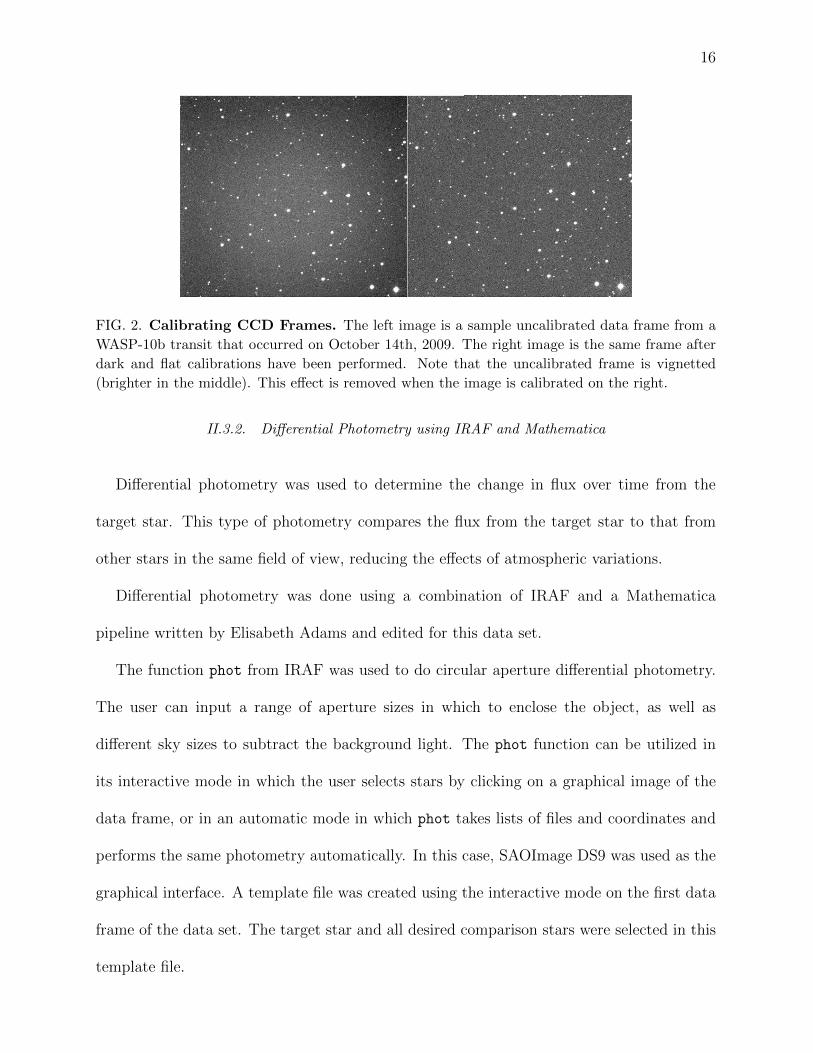
The dark-corrected frames are then divided by this normalized flat. An example of

uncalibrated and calibrated CCD frames is shown in Figure 2.

1 Image Reduction and Analysis Facility. National Optical Astronomy Observatory. http://iraf.noao.edu/

16

FIG. 2. Calibrating CCD Frames. The left image is a sample uncalibrated data frame from aWASP-10b transit that occurred on October 14th, 2009. The right image is the same frame afterdark and flat calibrations have been performed. Note that the uncalibrated frame is vignetted(brighter in the middle). This effect is removed when the image is calibrated on the right.

II.3.2. Differential Photometry using IRAF and Mathematica

Differential photometry was used to determine the change in flux over time from the

target star. This type of photometry compares the flux from the target star to that from

other stars in the same field of view, reducing the effects of atmospheric variations.

Differential photometry was done using a combination of IRAF and a Mathematica

pipeline written by Elisabeth Adams and edited for this data set.

The function phot from IRAF was used to do circular aperture differential photometry.

The user can input a range of aperture sizes in which to enclose the object, as well as

different sky sizes to subtract the background light. The phot function can be utilized in

its interactive mode in which the user selects stars by clicking on a graphical image of the

data frame, or in an automatic mode in which phot takes lists of files and coordinates and

performs the same photometry automatically. In this case, SAOImage DS9 was used as the

graphical interface. A template file was created using the interactive mode on the first data

frame of the data set. The target star and all desired comparison stars were selected in this

template file.

17

The midtime of each data file was extracted from the header file of each data frame. The

template file generated by phot was then sent to the Mathematica pipeline. A centroiding

algorithm adjusted the position of each star over time to account for imperfections in the

tracking of the telescope. The pipeline returned a list of these recentered coordinates.

The IRAF function phot was used again, this time in its automatic mode. It read in these

recentered coordinates for each data file, and returned a list of the instrumental magnitudes

of the targets and comparison stars. These values included the magnitudes of the target

and between 5 and 20 different comparison stars for each of the aperture sizes used, ranging

from 3 pixels to 14 pixels in half steps. The sky to be subtracted from the region within this

aperture was calculated using a larger annulus around each star with an inner radius input

by the user.

After this, the data reduction was completed using Mathematica to produce a light curve

of the magntitude ratio between the target and several chosen comparison stars. The values

from the IRAF differential photometry were sent to the Mathematica pipeline. The ratio of

the target to each comparison star in each aperture was calculated. The best aperture size

was chosen based on calculations that minimized the scatter on points. Comparison stars

that had saturated frames, too few counts, or unexplained variability in their magnitudes

were eliminated. The light curve output for each data set was made by adding the contri-

butions from each comparison star and using the ratio between the target and the sum of

the comparison magnitudes. Combining stars increases photon counts, decreasing statistical

uncertainty.

If the light curve had an anomaly in the baseline, some ‘detrending’ is possible. For

instance, the anomaly could be approximately proportional to the geometric diameter of

the observed star, which fluctuates due to variability in the seeing; instead, it could be

18

proportional to airmass because of differential extinction of the image over many hours.

The light curve can be ‘detrended’ using a linear detrending function against geometric

diameter, airmass, the x and y coordinates of the target star, or time. The function plots

time versus any one of these parameters and calculates the slope. The data points are then

scaled by this slope, reducing the anomaly in the baseline. This process can be repeated to

detrend against other of these features present in the light curve. Many of the six light curves

presented did not require detrending. Detrending of those that required it is explained in

Section IV.

19

II.4. Transit Fitting

II.4.1. Least Squares Fit

The models were fit using a least squares fitting Mathematica package from Jim Elliot’s

research group at MIT. Eight different parameters were used to make this least squares fit.

These parameters were the scale (the number that will normalize the baseline to 1), the

slope, the midtime of the transit, the duration of the transit, the ratio of the radii of the

planet and star, the impact parameter, and two limb darkening parameters. These could

not all be constrained with the data from Wallace Observatory, leading to assumptions in

the fit for each light curve. Different parameters were taken to be constant based on the

quality of the light curve.

For all transits, the impact parameter was calculated using results from published papers.

The impact parameter b is defined by the equation

b = cos i · a

Rstar, (1)

where i is the orbital inclination, a is the semi-major axis, and Rstar is the stellar radius.

The value of the semi-major axis a can be determined from the shape of the transit light

curve. The inclination can be determined using the equation

tT =PR�

πa

�(1 +

Rp

R�

)2 − (a

R�

cos i)2, (2)

where tT is the transit duration and Rp is the radius of the planet (Seager 2008). The

impact parameter for the fit was calculated for each transit with published values for these

20

parameters.

The other two values taken to be constant for all light curves were the two limb dark-

ening parameters. These were calculated using a FORTRAN program written by John

Southworth called jktld which accepts values for the effective temperature, surface grav-

ity, metal abundance [M/H], and microturbulence velocity and returns values for various

linear and nonlinear models for limb darkening2. For this fit, two quadratic limb darkening

parameters are used.

The impact parameter and two limb darkening parameters were kept constant for all

transit fits. In addition, values for transit duration or slope were also held constant if the

transit light curve could not constrain the model well enough to fit them. The models were

fit to the parameters not held constant: the scale, midtime of the transit, and the ratio

of the planetary radius to the stellar radius were calculated for all light curves. (Transit

duration and slope were calculated for some light curves). The initial values of the midtime

and scale were estimated and input by the user; the initial values for the radius ratio and

transit duration were literature values. The least squares fit algorithm iterated these initial

values until they converged on a set of values that minimized the sum of the squared resid-

uals between the model and the data. The fitting software returned the values for these

parameters and the errors on the parameters from this residual of the fit.

II.4.2. Calculating Parameters using Least Squares Fit

The radius of the planet can be calculated using the ratio of the planetary radius to the

stellar radius. This ratio RPR�

will be defined symbolically as δ. The planetary radius is

2 Southworth, John. JKTLD - for calculating limb darkening coefficients.

http://www.astro.keele.ac.uk/ jkt/codes/jktld.html

21

Rp =RP

R�

·R� = δ ·R� (3)

with an error of

∆Rp =�

δ2 · (∆R�)2 +R2�· (∆δ)2), (4)

where ∆δ is the error in the radius ratio from the least squares fit, ∆R� is the error in the

radius of the star (Johnson et al. 2009), and ∆Rp is the error on the radius of the planet.

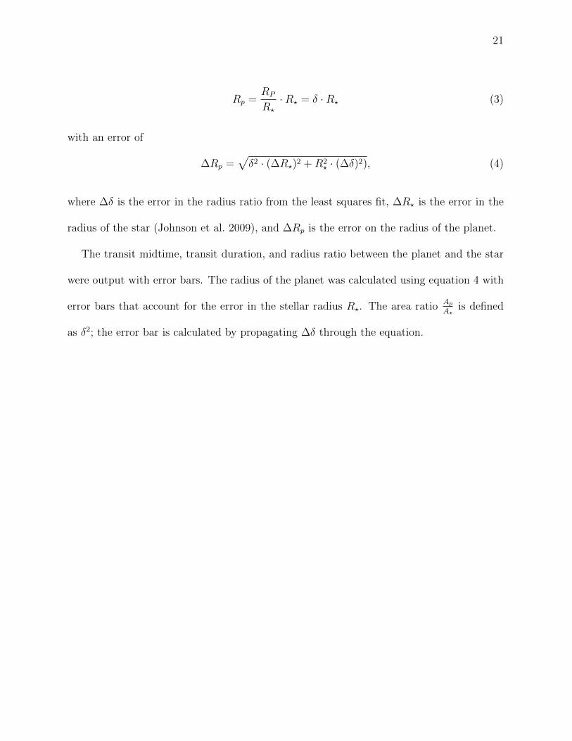
The transit midtime, transit duration, and radius ratio between the planet and the star

were output with error bars. The radius of the planet was calculated using equation 4 with

error bars that account for the error in the stellar radius R�. The area ratio Ap

A�is defined

as δ2; the error bar is calculated by propagating ∆δ through the equation.

22

III. OBSERVATIONS

Observations of the three planets discussed in the Introduction (TrES-3, WASP-10b,

and WASP-11/HAT-P-10b) were taken between June 2009 and January 2010. Many other

observations of other planets including HAT-P-5b, HAT-P-7b, HD17156b, HD80606b, and

HAT-P-11b were attempted, but the data were discarded for a variety of reasons summarized

in Table XVIII. Discussion of the difficulties experienced observing fromWallace Observatory

and the viability of exoplanet research from small observatories will follow in Section VII.

TABLE VII. Reasons for Exclusion of other Transit Data

Planet Date Reason for Exclusion

TrES-3 2009/07/21 The night became extremely cloudy. Data were examined and imageswith fewer than 10,000 counts on the target star were excluded. This leftapproximately 20 data frames left, which were not sufficient to create areasonable light curve.

HAT-P-5b 2009/07/07 It was hazy and the moon was extremely bright (it was a nearly fullmoon close to my target). The counts on the target star dropped duringthe night. Only a partial transit was observed.

HAT-P-7b 2009/07/10 It was clear at the beginning of the night but became cloudy. Onlya partial transit was observed. In addition, the HAT-P-7b transit isshallow (0.7%) which decreased the signal to noise ratio considerably.

WASP-3b 2009/07/14 Thick clouds rolled after 30 minutes of observation. Transit was notobserved.

HD17156b 2009/07/20 Observed by Robert Arlt. The night seemed to be reasonably clear;counts dropped off towards morning. The main limiting factor here isthe lack of comparison stars - HD17156 is a bright star (8.17 mag) withno really comparable stars in the field. We needed 5 sec exposures toavoid saturating the target, but this meant that dimmer stars had veryfew counts. I used the brightest 2 stars to make this plot.

HAT-P-11b 2009/08/02 Transit was only 0.3% deep. Signal to noise ratio was extremely low,and transit was not visible within the noise.

HD80606b 2009/01/14 Observed as part of a coalition of observers organized by Josh Winn.Weather conditions at Wallace Observatory were variable and a smallpart of the transit was observed (part of egress plus a small amount ofbaseline afterwards). The light curve was sent to collaborators, but isnot complete enough by itself for inclusion in this work.

23

III.1. TrES-3 Observations

Usable data from TrES-3 were collected on June 17th, 2009 and on July 4th, 2009. TrES-

3 was a good target from Wallace Observatory for a few reasons. First, it has excellent

comparison stars. Second, it is a deep transit (2.6% deep), which significantly increases

the signal to noise ratio. Third, I had reasonably good weather for both transits. These

observations are summarized in Table VIII. An example star field is shown in Figure 3.

FIG. 3. Example TrES-3 Field. This image was taken on June 17th, 2009 and has beencalibrated using flat and dark images from the same night. TrES-3 is circled in green. Comparisonstars used for differential photometry are circled in magenta.

On June 17th, my very first night of observing ever, the weather was especially clear.

Flats, darks, and biases were collected before observations began. The R filter was used and

24

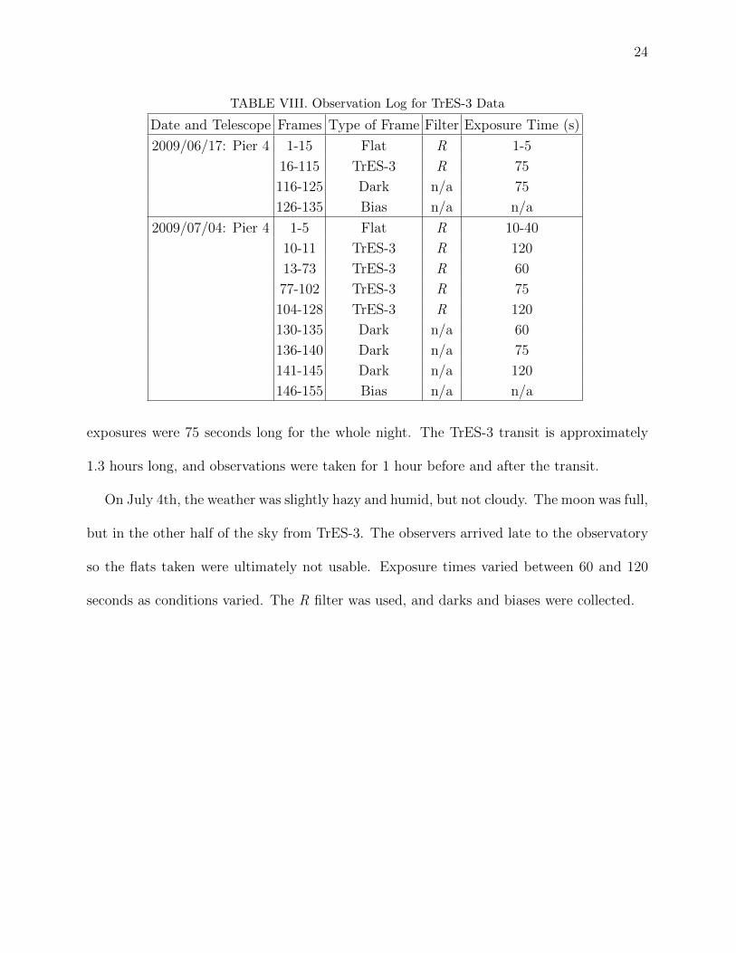
TABLE VIII. Observation Log for TrES-3 Data

Date and Telescope Frames Type of Frame Filter Exposure Time (s)

2009/06/17: Pier 4 1-15 Flat R 1-5

16-115 TrES-3 R 75

116-125 Dark n/a 75

126-135 Bias n/a n/a

2009/07/04: Pier 4 1-5 Flat R 10-40

10-11 TrES-3 R 120

13-73 TrES-3 R 60

77-102 TrES-3 R 75

104-128 TrES-3 R 120

130-135 Dark n/a 60

136-140 Dark n/a 75

141-145 Dark n/a 120

146-155 Bias n/a n/a

exposures were 75 seconds long for the whole night. The TrES-3 transit is approximately

1.3 hours long, and observations were taken for 1 hour before and after the transit.

On July 4th, the weather was slightly hazy and humid, but not cloudy. The moon was full,

but in the other half of the sky from TrES-3. The observers arrived late to the observatory

so the flats taken were ultimately not usable. Exposure times varied between 60 and 120

seconds as conditions varied. The R filter was used, and darks and biases were collected.

25

III.2. WASP-10b Observations

WASP-10 was observed for 4.5 hours, from 01:35 to 06:05 (UT) on October 14, 2009.

The weather was clear and crisp. Twilight flats were obtained after the transit, during the

evening of the 14th. Images were collected on two telescopes in two different filters. The I

filter was used on Pier 4 and the V filter was used on Pier 3. Exposure times were varied

as the seeing changed during the course of the night from 2 minutes to 3 minutes and 30

seconds. These observations are summarized in Table IX. An example star field is shown in

Figure 4.

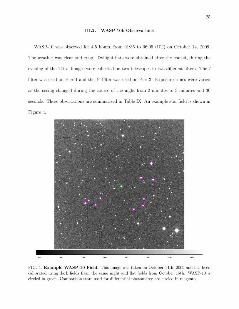
FIG. 4. Example WASP-10 Field. This image was taken on October 14th, 2009 and has beencalibrated using dark fields from the same night and flat fields from October 15th. WASP-10 iscircled in green. Comparison stars used for differential photometry are circled in magenta.

26

TABLE IX. Observation Log for WASP-10b Data

Date andTelescope Frames Type of Frame Filter Exposure Time (s)

2009/10/14: Pier 3 13-33 WASP-10b V 150

34-94 WASP-10b V 210

95-99 Dark n/a 210

100-194 Dark n/a 150

105-124 Bias n/a n/a

2009/10/14: Pier 4 1-10 Dark n/a 60

19-40 WASP-10b I 150

41-101 WASP-10b I 210

102-107 Dark n/a 210

108-112 Dark n/a 150

113-133 Bias n/a n/a

27

III.3. WASP-11/HAT-P-10b Observations

WASP-11/HAT-P-10b was observed for 5.5 hours from 22:30 on January 20th to 04:00

(UT) on January 21st, 2010 using both Pier 3 and Pier 4. The weather was reasonably

clear, and the seeing was slightly variable. Flats were obtained during the evening before

the transit. The exposure time was varied between 60 seconds and 90 seconds. The R filter

was used in Pier 3 and Pier 4. Images were collected on Pier 4 for the entire 5.5 hour period.

Images were collected on Pier 3 for about two thirds of the 5.5 hour transit period, with a

section in the middle missing because of observer error. The observer forgot to save files

automatically after the meridian flip and thus lost data between the meridian flip and the

time at which she realized and fixed the mistake. These observations are summarized in

Table X. An example star field is shown in Figure 5.

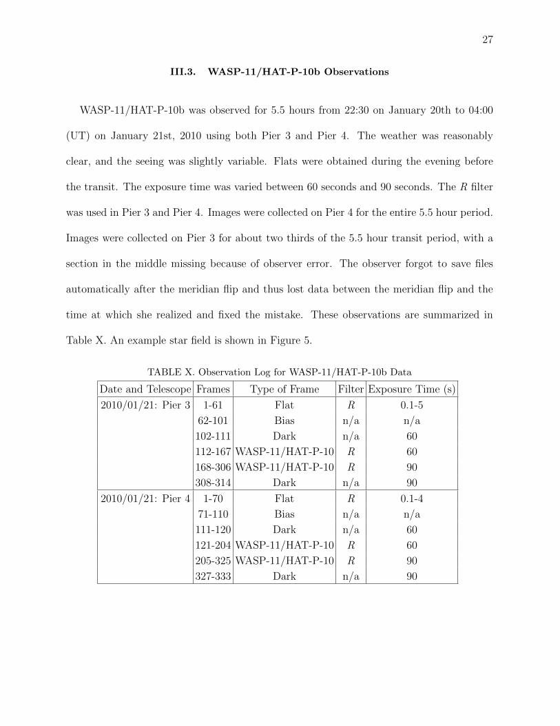
TABLE X. Observation Log for WASP-11/HAT-P-10b Data

Date and Telescope Frames Type of Frame Filter Exposure Time (s)

2010/01/21: Pier 3 1-61 Flat R 0.1-5

62-101 Bias n/a n/a

102-111 Dark n/a 60

112-167 WASP-11/HAT-P-10 R 60

168-306 WASP-11/HAT-P-10 R 90

308-314 Dark n/a 90

2010/01/21: Pier 4 1-70 Flat R 0.1-4

71-110 Bias n/a n/a

111-120 Dark n/a 60

121-204 WASP-11/HAT-P-10 R 60

205-325 WASP-11/HAT-P-10 R 90

327-333 Dark n/a 90

28

FIG. 5. Example WASP-11/HAT-P-10b Field. This image was taken on January 21st, 2010and has been calibrated using flat and dark images from the same night. WASP-11/HAT-P-10 iscircled in green. Comparison stars used for differential photometry are circled in magenta.

29

IV. DATA REDUCTION FOR OBSERVED TRANSITS

The general methods of data reduction are described in Section II.3. Each individual

transit had certain deviations from the general methods that will be described in this section.

IV.1. TrES-3 Data Reduction

IV.1.1. 2009/06/17

Differential photometry for this transit used 9 comparison stars (shown above in Figure

3. The aperture size was 4.75 pixels (6 arcseconds), the sky inner radius was 17 pixels

(22 arcseconds), and outer radius was 33 pixels (43 arcseconds). Frames with under 25,000

counts on the target star were removed; counts declined sharply about two thirds of the

way through the transit, so the last half of the transit is noisier than the first half of the

transit). The transit was detrended linearly with the geometric diameter of the target star;

this detrending improved photometric precision slightly, from 2.5 mmag to 2.01 mmag.

IV.1.2. 2009/07/04

As discussed before, flats from 2009/07/04 were unusable. Instead, calibrations were

done using flats from 2009/06/17. Differential photometry for this transit used 5 stars.

The aperture size chosen was 4.0 pixels (5 arcseconds), the sky inner radius was 20 pixels

(26 arcseconds), and the outer radius was 40 pixels (52 arcseconds). Frames with under

25,000 counts on the target star were removed. This essentially took out a cloudy middle

section of the transit including ingress and the flat part after egress, leaving me with baseline

before ingress and almost all of egress. The section after the meridian flip may have been

30

troublesome because flats from 2 weeks prior were used; this means that the fields are

not completely flat because of changes in the dust and alignment of the telescope. The

photometric precision of this transit was 5.44 mmag.

IV.2. WASP-10b Data Reduction

Differential photometry for WASP-10b used ten comparison stars. For both the Pier 3

and Pier 4 data, the best aperture size was 6.5 pixels (8.4 arcseconds). The sky annulus

chosen had an inner radius of 25 pixels (32 arcseconds) and an outer radius of 50 pixels (65

arcseconds). The Pier 4 light curve had a slight slope that was correlated with the geometric

diameter and was detrended to correct for this slope. The Pier 3 light curve did not have

this slope and was not detrended against any parameters.

IV.3. WASP-11/HAT-P-10b Data Reduction

Differential photometry for WASP-11/HAT-P-10b used seven comparison stars. The

aperture size chosen for both the Pier 3 and Pier 4 data was 5.5 pixels (7 arcseconds). The

sky annulus had an inner radius of 30 pixels (39 arcseconds) and an outer radius of 60 pixels

(77 arcseconds). The Pier 3 light curve is missing the middle section because of human error

while observing (see Section III.3). The photometric precisions of the Pier 3 and Pier 4 light

curves were 3.55 mmag and 3.86 mmag respectively.

31

V. FITTING LIGHT CURVES

V.1. TrES-3

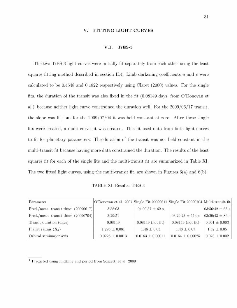
The two TrES-3 light curves were initially fit separately from each other using the least

squares fitting method described in section II.4. Limb darkening coefficients u and v were

calculated to be 0.4548 and 0.1822 respectively using Claret (2000) values. For the single

fits, the duration of the transit was also fixed in the fit (0.08149 days, from O’Donovan et

al.) because neither light curve constrained the duration well. For the 2009/06/17 transit,

the slope was fit, but for the 2009/07/04 it was held constant at zero. After these single

fits were created, a multi-curve fit was created. This fit used data from both light curves

to fit for planetary parameters. The duration of the transit was not held constant in the

multi-transit fit because having more data constrained the duration. The results of the least

squares fit for each of the single fits and the multi-transit fit are summarized in Table XI.

The two fitted light curves, using the multi-transit fit, are shown in Figures 6(a) and 6(b).

TABLE XI. Results: TrES-3

Parameter O’Donovan et al. 2007 Single Fit 20090617 Single Fit 20090704 Multi-transit fit

Pred./meas. transit time1 (20090617) 3:58:03 04:00:37 ± 62 s 03:56:42 ± 63 s

Pred./meas. transit time1 (20090704) 3:29:51 03:29:23 ± 114 s 03:29:43 ± 86 s

Transit duration (days) 0.08149 0.08149 (not fit) 0.08149 (not fit) 0.061 ± 0.003

Planet radius (RJ) 1.295 ± 0.081 1.46 ± 0.03 1.48 ± 0.07 1.32 ± 0.05

Orbital semimajor axis 0.0226 ± 0.0013 0.0163 ± 0.00011 0.0164 ± 0.00025 0.023 ± 0.002

1 Predicted using midtime and period from Sozzetti et al. 2009

32

V.2. WASP-10b

The two WASP-10b light curves were fit separately using the least squares fitting method

described in section II.4. Limb darkening coefficients were different for each light curve

because the data were taken using different filters. For Pier 3 (V filter), values of u and v

were 0.7657 and 0.0743. For Pier 4 (I filter), values of u and v were 0.4230 and 0.2693 using

Claret (2000) values. The slopes were taken to be zero, and the light curves were fit for the

four remaining parameters (radius ratio, duration, midtime, and scale). A multi-curve fit

was not completed because the limb darkening coefficients were different for each light curve.

The values found in each fit were then combined using a weighted average. The results of

the least-squares fit for each of the single fits and the combined values using both fits are

shown in Table XII. The two fitted light curves are shown in Figures 7(a) and 7(b).

TABLE XII. Results: WASP-10b

Parameter Johnson et al. 2008 Pier 3 (V Filter) Pier 4 (I Filter) Combined Value

Pred./Meas. Midtime (h:min:s)2 4:02:44 4:03:53 ±38 4:03:34 ±35s 4:03:18 ± 26s

Transit Duration (hours) 2.2271+0.0078−0.0068 2.31 ±0.03 2.39 ±0.03 2.35 ±0.02

Planet/Star Area Ratio 0.02525 +0.00024−0.00028 0.0252 ±0.0008 0.0294 ±0.0008 0.0272 ±0.0006

Radius of Planet (RJ) 1.080± 0.020 1.08 ±0.02 1.17 ±0.03 1.12 ±0.02

V.3. WASP-11/HAT-P-10b

The two WASP-11/HAT-P10b light curves were fit separately using the least squares

fitting method described in section II.4. They were then fit using the multi-transit fitting

model. Limb darkening coefficients u and v were calculated to be 0.6411 and 0.1441 respec-

tively. The slopes were taken to be zero, and the light curves were fit for the four remaining

2 Predicted using midtime and period from Johnson et al., 2009

33

parameters (radius ratio, duration, midtime, and scale). A multi-curve fit was then com-

pleted, fitting both plots with the same model. The results of the least-squares fit for each

of the single fits and the multi-fit values are shown in Table XIII. The two fitted light curves

are shown in Figures 8(a) and 8(b).

TABLE XIII. Results: WASP-11/HAT-P-10b

Parameter Bakos et al. 2008 Pier 4 Pier 3 Multi-fit

Predicted/measured 01:17:21 01:16:06 ± 74s 01:15:56 ± 179s Pier 4: 01:15:58±111s

transit time (h:m:s)3 Pier 3: 01:16:56±129s

Transit duration (days) 0.1100 ± 0.0015 0.108 ± 0.002 0.111 ±0.005 0.111±0.004

Planet radius (RJ) 1.045 +0.050−0.033 1.106 ±0.02 1.077 ± 0.03 1.115 ±0.049

Orbital semimajor axis 0.0439+0.0006−0.0009 0.045 ± 0.001 0.0442 ±0.002 0.0415±0.002

3 Predicted using midtime and period from Bakos et al. 2008

34

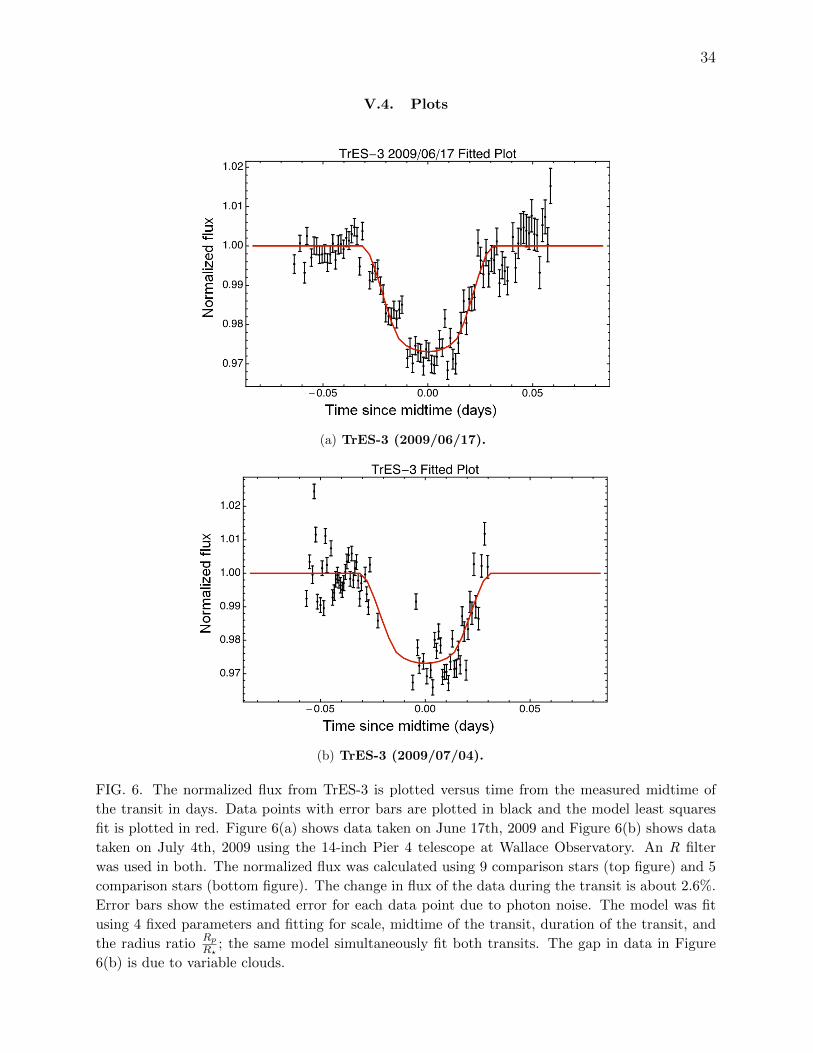
V.4. Plots

(a) TrES-3 (2009/06/17).

(b) TrES-3 (2009/07/04).

FIG. 6. The normalized flux from TrES-3 is plotted versus time from the measured midtime ofthe transit in days. Data points with error bars are plotted in black and the model least squaresfit is plotted in red. Figure 6(a) shows data taken on June 17th, 2009 and Figure 6(b) shows datataken on July 4th, 2009 using the 14-inch Pier 4 telescope at Wallace Observatory. An R filterwas used in both. The normalized flux was calculated using 9 comparison stars (top figure) and 5comparison stars (bottom figure). The change in flux of the data during the transit is about 2.6%.Error bars show the estimated error for each data point due to photon noise. The model was fitusing 4 fixed parameters and fitting for scale, midtime of the transit, duration of the transit, andthe radius ratio Rp

R�; the same model simultaneously fit both transits. The gap in data in Figure

6(b) is due to variable clouds.

35

(a) WASP-10b (V Filter).

(b) WASP-10b (I Filter).

FIG. 7. The normalized flux from WASP-10 is plotted versus time from the measured midtime ofthe transit in days. Data points with error bars are plotted in black and the model least squaresfit is plotted in purple or red. Residuals are plotted offset from the light curve. Both plots showdata taken on October 14th, 2009 on 14-inch telescopes at Wallace Observatory; the data in thetop plot were taken on Pier 3 and the data in the bottom plot were taken on Pier 4. A V filterwas used on Pier 3 and an I filter was used on Pier 4. The normalized flux was calculated using10 comparison stars. The change in flux of the data during the transit is about 2.5%. Error barsshow the estimated error for each data point due to photon noise. The model was fit using 4 fixedparameters and fitting for scale, midtime of the transit, duration of the transit, and the radiusratio Rp

R�; the same model simultaneously fit both transits.

36

(a) WASP-11/HAT-P-10b (Pier 3).

(b) WASP-11/HAT-P-10b (Pier 4).

FIG. 8. The normalized flux from WASP-11/HAT-P-10 is plotted versus time from the measuredmidtime of the transit in days. Data points with error bars are plotted in black and the modelleast squares fit is plotted in blue. Both plots show data taken on January 21st, 2010 on 14-inchtelescopes at Wallace Observatory; the data in the top plot were taken on Pier 3 and the data inthe bottom plot were taken on Pier 4. The R filter was used in Pier 3 and Pier 4. The exposuretime was varied between 60 seconds and 120 seconds. The normalized flux was calculated using7 comparison stars. The change in flux of the data during the transit is about 1.8%. Error barsshow the estimated error for each data point due to photon noise. The model was fit using 4 fixedparameters and fitting for scale, midtime of the transit, duration of the transit, and the radiusratio Rp

R�; the same model simultaneously fit both transits.

37

VI. TRANSIT TIMING VARIATIONS (TTV)

VI.1. Comparing Measured Transit Midtimes with Literature Midtime Values

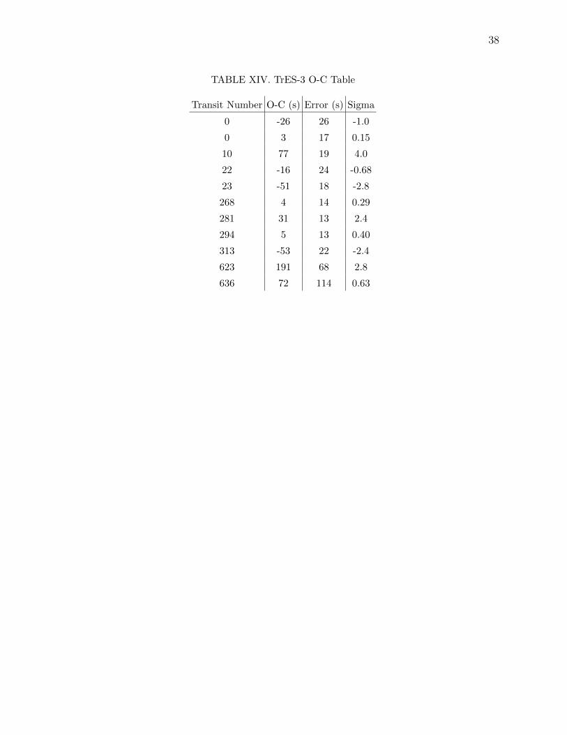
The deviations from predicted transit time are shown in Tables XIV, XV, and XVI and

are shown graphically in the ‘O-C’ Figures 9, 10, and 11. These plots show the epoch of

the known transit (including literature values) plotted against the observed time minus the

calculated time. The code used to measure transit times and generate the plots in this

section was adapted from Elisabeth Adam’s transit timing code (Adams, 2010).

VI.1.1. TrES-3 TTV

As you can see, the O-C plot for TrES-3 shows that my first observed transit deviates from

the calculated time by 191 seconds (2.8 sigma). Some of this difference could potentially

be due to differences in calculating time in BJD. Some groups use calculations that include

additional leap seconds (the code used for these calculations does) but other groups do

not. (See discussion in Appendix C of Adams, 2010 for a detailed explanation of conversion

between UTC and TT). The offset for all of these transits is 66.187 seconds (Adams, 2010).

Whether other scientists used this offset in their calculations is difficult to determine without

talking to the other groups. My second transit deviates from the calculated time by 72

seconds, which agrees within 1 sigma of the calculated time.

38

TABLE XIV. TrES-3 O-C Table

Transit Number O-C (s) Error (s) Sigma

0 -26 26 -1.0

0 3 17 0.15

10 77 19 4.0

22 -16 24 -0.68

23 -51 18 -2.8

268 4 14 0.29

281 31 13 2.4

294 5 13 0.40

313 -53 22 -2.4

623 191 68 2.8

636 72 114 0.63

39

�

�

�

�

��

���

��

Sozzetti et al. �2008� ephemeris

0 100 200 300 400 500 600�300

�200

�100

0

100

200

300

orbital periods

O�C�sec�

�

��

�

��

���

�

�

New ephemeris

0 100 200 300 400 500 600�300

�200

�100

0

100

200

300

orbital periods

O�C�sec�

FIG. 9. TrES-3 O minus C Graph. This plot shows the literature midtimes of TrES-3 transitsfrom O’Donovan et al. (2007) and Sozzetti et al. (2008). In the top plot, the period and firstmidtime in Sozzetti et al. (2008) was used as the baseline. The diagonal lines represent 1 sigma and2 sigma deviations from the calculated transit time using the published error on the period. Notethat Sozzetti’s points and O’Donovan’s points agree reasonably well with this ephemeris, thoughit seems that they have perhaps underestimated errors. Transits from this work are shown in blue.In the bottom plot the ephemeris is recalculated, incorporating all published midtimes plus thosemeasured in this project. This changes the period slightly, but it greatly increases the error on theperiod.

40

VI.1.2. WASP-10b TTV

WASP-10b had the smallest statistical error bars on the timing, but the largest systematic

offset from the calculated time. Note that O-C for the Pier 3 and Pier 4 were 217±35 seconds

and 237±38 seconds (See Table XV and Figure 10). This could mean that a transit timing

variation was detected. However, the same transit (epoch 0) was also observed by Dittmann

et al. using the 61-inch Kuiper telescope on Mt. Bigelow and a clock that synchronized

with GPS every few seconds (Dittmann 2010). Dittmann et al.’s value agrees very well

with Christian et al. and Johnson et al.; it seems much more likely that there was some

kind of systematic error in the light curve timing. One possibility is that the clock was not

synchronized correctly. Another possibility is that there is a systematic error in the code

that determines the timing. Preliminary fits on the data kindly provided by J Dittman

(personal communication) indicate that when we fit his data using our model we do not

find the same times he did, with an O-C of 469 seconds. This discrepancy is still being

investigated.

TABLE XV. WASP-10b O-C Table

Transit Number O-C (s) Error (s) Sigma

-246 -15 35 -0.41

-147 6 7 0.78

-111 230 69 3.3

-14 27 9 3.1

-3 244 26 9.4

-2 190 26 7.3

0 217 35 6.2

0 237 38 6.2

0 0 11 0

41

��

��

�

�

�

�

�

Dittmann et al. �2010� ephemeris

�250 �200 �150 �100 �50 0�100

0

100

200

300

orbital periods

O�C�sec�

��

��

�

�

�

�

�

New ephemeris

�250 �200 �150 �100 �50 0�100

0

100

200

300

orbital periods

O�C�sec�

FIG. 10. WASP-10b O minus C Graph. This plot shows the literature midtimes of WASP-10btransits from Christian et al. (2008), Johnson et al. (2009), Krejcova et al. (2010), and Dittmannet al. (2010). In the top plot, the period and midtime in Dittmann et al. (2010) was used asthe baseline. The diagonal lines represent 1 sigma and 2 sigma deviations from the calculatedtransit time using the published error on the period. Note that Christian’s points and Johnson’spoints agree very well with this ephemeris; Krejcova’s published points vary. The midtimes fromthis study are shown in blue, and deviate significantly from the ephemeris in the literature. Inthe bottom plot the ephemeris is recalculated, incorporating all published midtimes plus thosemeasured in this project. This changes the period slightly, but it greatly increases the error on theperiod.

42

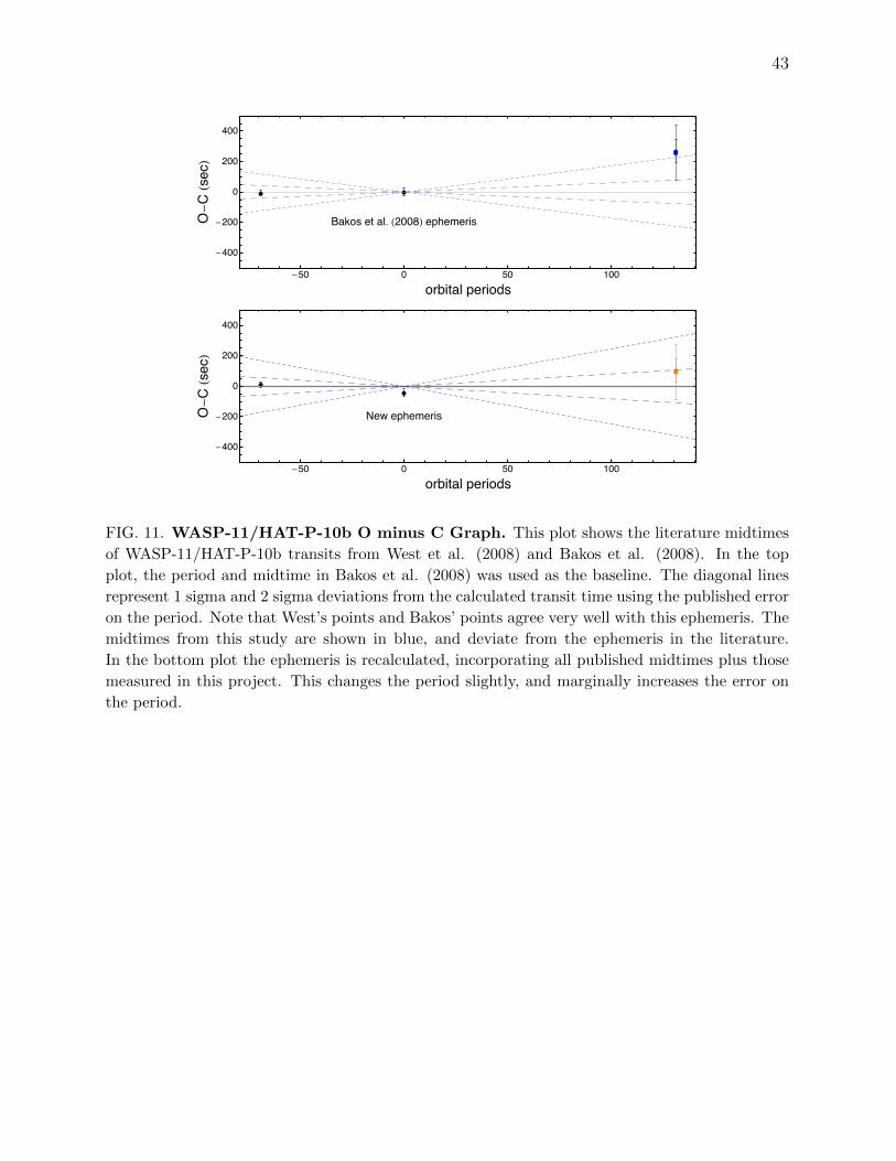
VI.1.3. WASP-11/HAT-P-10b TTV

The observed midtimes for WASP-11/HAT-P-10b are plotted with the two published

midtimes. The first is from West et al. (2008), the WASP discovery paper. The second

is from Bakos et al. (2008), the HAT discovery paper. The light curves from this paper

deviate from the ephemeris from Bakos et al. by 257±179 seconds (for the partial transit,

observed on Pier 3) and 268±74 seconds (for the full transit, observed on Pier 4).

TABLE XVI. WASP-10b O-C Table

Transit Number O-C (sec) Error (sec) Sigma

-69 -8 17 -0.44

0 0 26 0

131 257 179 1.4

131 268 74 3.6

43

��

��

Bakos et al. �2008� ephemeris�50 0 50 100

�400

�200

0

200

400

orbital periods

O�C�sec�

��

��

New ephemeris

�50 0 50 100

�400

�200

0

200

400

orbital periods

O�C�sec�

FIG. 11. WASP-11/HAT-P-10b O minus C Graph. This plot shows the literature midtimesof WASP-11/HAT-P-10b transits from West et al. (2008) and Bakos et al. (2008). In the topplot, the period and midtime in Bakos et al. (2008) was used as the baseline. The diagonal linesrepresent 1 sigma and 2 sigma deviations from the calculated transit time using the published erroron the period. Note that West’s points and Bakos’ points agree very well with this ephemeris. Themidtimes from this study are shown in blue, and deviate from the ephemeris in the literature.In the bottom plot the ephemeris is recalculated, incorporating all published midtimes plus thosemeasured in this project. This changes the period slightly, and marginally increases the error onthe period.

44

VI.2. Potential for Exomoon detection using Small Telescopes

In this section, the potential for exomoon discovery around TrES-3, WASP-10b, and

WASP-11/HAT-P-10b will be quantified. The maximum transit timing variation that could

be induced by an orbiting moon around a planet was calculated for a moon in a circular

orbit around a planet which is in a circular orbit about its star. The calculations also assume

there were no other perturbing influences (such as another planet) in the system. I started

with Kepler’s Third Law, which states

P 2 =4π2a3

G(Ms +Mp), (5)

where a is the semi-major axis of the planet, Mp is the mass of the planet, Ms is the

mass of the star, P is the period of the orbit, and G is the gravitational constant. The

planet-moon system will rotate about its center of mass, which is located at

rcm =dmoonMmoon

Mp +Mmoon, (6)

where rcm is the distance from the planet to the center of mass, dmoon is the distance from

the planet to the moon, and Mmoon is the mass of the exomoon. The maximum distance the

planet could be “ahead” or “behind” in its orbit would be equal to 2rcm. I then set the ratio

of the perturbation in distance to the total distance equal to the ratio of the perturbation

in time to the period as follows:

2rcm2πa

=TTV

P, (7)

where TTV is the maximum transit timing variation. From equations 5, 6, and 7, I determine

45

that the maximum TTV is

TTV =2dmoona1/2

(Mp +Mmoon)G1/2(Ms +Mp)1/2. (8)

For a moon to be gravitationally bound to the planet, it must orbit within the Hill sphere

of a planet. The radius of the Hill sphere is given by the equation

rHill =amp

3M1/3∗

. (9)

Moons orbiting inside the Hill sphere can be in stable orbits. Moons will not be found

outside of the Hill sphere.

The precision of transit timing from Wallace for each transit was input as the TTV in

this equation. The only unknowns in the equations are then mmoon and dmoon. Figures 12,

13, and 14 show plots of the mass of a potential moon versus the radius at which a moon

of that mass could be detected. The solid green line represents a 3σ detection. The dotted

blue and magenta lines represent 2σ and 1σ detections. The shaded purple region above

the green curve represents the region of detectable moons. The radius of the Hill sphere for

each planet is plotted with a solid horizontal red line. The shaded red region under the red

line represent the region of stable moon orbits.

For TrES-3 and WASP-10b, the region of detectable moons does not overlap with the

region of stable orbits; moons under 10 Earth Masses could not be detectable using the

Wallace telescopes. For WASP-11/HAT-P-10b, the region of detectable moons actually

overlaps with the region of stable orbits; moons around six earth masses orbiting close to

the planet’s Hill Sphere could be detectable using the Wallace telescopes or other similar

amateur telescopes.

46

FIG. 12. TrES-3 Detectable Moons In this figure, the mass of a potential moon is plottedagainst the radius at which that sized moon could be detected. The solid green line representsa 3σ detection. The dotted blue and magenta lines represent 2σ and 1σ detections. The shadedpurple region above the green curve represents the region of detectable moons. The radius of theHill Sphere for each planet is plotted with a solid horizontal red line. The shaded red region underthe red line represent the region of potentially stable moon orbits. The mass range is from 0 to 10Earth masses. Clearly for TrES-3, the region of detectable moons does not overlap with the regionof stable orbits; moons under 10 Earth Masses will not be detectable using the Wallace telescopes.

47

FIG. 13. WASP-10b Detectable Moons In this figure, the mass of a potential moon is plottedagainst the radius at which that sized moon could be detected. The solid green line representsa 3σ detection. The dotted blue and magenta lines represent 2σ and 1σ detections. The shadedpurple region above the green curve represents the region of detectable moons. The radius of theHill Sphere for each planet is plotted with a solid horizontal red line. The shaded red region underthe red line represent the region of potentially stable moon orbits. The mass range is from 0 to 10Earth masses. For WASP-10b, the region of detectable moons does not overlap with the region ofstable orbits; moons under 10 Earth Masses will not be detectable using the Wallace telescopes.

48

FIG. 14. WASP-11/HAT-P-10b Detectable Moons In this figure, the mass of a potentialmoon is plotted against the radius at which that sized moon could be detected. The solid greenline represents a 3σ detection. The dotted blue and magenta lines represent 2σ and 1σ detections.The shaded purple region above the green curve represents the region of detectable moons. Theradius of the Hill Sphere for each planet is plotted with a solid horizontal red line. The shadedred region under the red line represent the region of potentially stable moon orbits. The massrange is from 0 to 10 Earth masses. For WASP-11/HAT-P-10b, the region of detectable moonsactually overlaps with the region of stable orbits; moons around six earth masses orbiting close tothe planet’s Hill Sphere could be detectable using the Wallace telescopes.

49

VII. OBSERVING CHALLENGES FROM WALLACE OBSERVATORY

As shown in Table XVIII, many observations were attempted but only a handful were

successful enough to analyze to determine system parameters. In this section, the challenges

of observing exoplanet transits fromWallace Observatory will be discussed. These challenges

mirror those of many enthusiastic amateur astronomers attempting to observe transits using

similar telescopes.

VII.1. Using Small Telescopes

The first challenge at Wallace is the size of the telescopes. I used two 14-inch telescopes

for almost all of my data collection (I briefly used the 24-inch telescope, but without much

luck because of poor weather conditions). These telescopes are similar in size to larger

amateur telescopes. A 14-inch telescope has only 12% of the collecting area of a 1-meter

telescope, or 0.3% of the collecting area of one of the 6.5 meter Magellan telescopes. This

means that a 14-inch telescope collects far fewer photons than larger telescopes. While most

stars with known exoplanets are plenty bright enough to be visible from these telescopes

(the observation limit for both 14-inch telescopes is around magnitude 18 and stars with

transits average about magnitude 12), the photon noise is much greater when fewer photons

are collected.

VII.2. Location in Massachusetts

Countless observations in Westford, Massachusetts were thwarted because of the weather.

Five out of seven transits discusses above in Table XVIII were omitted because of clouds or

other meteorological difficulties. Many other scheduled observation sessions were not even

50

attempted because of clouds, rain, or snow. This is much less of a problem with larger,

professional places because a location with better conditions is chosen.

Even when the weather is reasonable in Westford, the atmosphere is still a challenge.

The elevation of Wallace is about 107m above sea level (in comparison, Mauna Kea, which

has several telescopes, is 4,205 meters above sea level). Large telescopes are generally placed

on mountaintops so that there is less atmosphere above them. The low elevation of Wallace

means that the atmosphere has signficant extinction, seeing, dispersion, and scintillation

effects on astronomical observations. Background light is also a problem; Wallace is near

Boston, Lowell, and other urban and suburban locations.

VII.3. Examples of “Bad Data”

This section will illustrate some of the challenges encountered observing exoplanets from

Wallace by showing some omitted data.

51

FIG. 15. HAT-P-7b Transit. These data were taken on July 10th from Pier 3. This transitis probably the ‘best’ looking rejected transit. The transit is certainly visible, and is about 0.6%.It was omitted because clouds prevented the observation of egress and because the signal to noiseratio is low because the transit is so shallow. This data illustrates that transits shallower that 0.6%are much more challenging to observe from small telescopes, especially if conditions deteriorate.Note that this transit would have been fit and analyzed if an observation of a full transit had beenmade.

FIG. 16. HAT-P-11b Transit. These data were taken on August 2nd on the 24-inch telescope.There are some slightly odd systematic errors due to the non-flatness of the field, but this imageis included to illustrate the limits of observation from Wallace. The transit of HAT-P-11b is 0.3%deep. Even with the 24-inch telescope, the noise here is too great to actually detect a transit thisshallow.

52

FIG. 17. HD17156b Transit. These data were taken on July 20th on Pier 3. There is somesystematic slope. The transit of HD17156 is 0.5% deep. The limitation of this transit was not themagnitude of the target star but the magnitude of comparison stars; there were no comparablybright objects in the field. Comparison stars are challenging in this system because HD17156bis bright (V magnitude 8.17). Field of view limitations exist in all telescopes, and, in fact, the14-inch telescopes, with 22 arcminute fields of view, are generally adequate for transits becausemost stars with known transiting planets are dimmer (magnitude 12).

53

VIII. CONCLUSIONS

I have presented six new transit light curves for three planetary systems: WASP-10b,

TrES-3, and WASP-11/HAT-P-10b. The measured planetary radii and semi-major axes

agree to within 1-2 sigma with literature values for all transits. The measured parameters

are summarized in Table XVII.

TABLE XVII. Measured Planetary Parameters: Summary

Planet Radius (RJ) Semi-major Axis (AU) Transit Duration (days)

WASP-10b 1.12 ±0.02 0.0342±0.0005 0.0979 ±0.0008

WASP-11/HAT-P-10b 1.115 ±0.049 0.0415±0.002 0.111±0.004

TrES-3 1.32 ± 0.05 0.023 ± 0.002 0.061 ± 0.003

VIII.1. Observing Exoplanet Transits and Transit Timing Variations from Small

Telescopes

I have demonstrated that observing exoplanet transits from small telescopes in poor

weather sites can be very successful. The transit of WASP-11/HAT-P-10b had high enough

precision on its light curves to measure transit timing variations that could indicate a large

(6REarth+) exomoon in this system.

I have also discussed the difficulties of observing transits using small telescopes. Weather

conditions prevented quality observations more than 50% of the time (Out of 13 transits

observations were attempted, five were ultimately discarded due to weather; dozens of others

were planned but not attempted due to poor weather conditions). I determined that these 14-

inch telescopes do not have enough collecting area to collect useful data for shallow transits

(less than about 0.6%). This limitation would generally prevent the observation of most

54

small (Neptune and Earth sized) planets from Wallace and other small observatories. Some

small planets could be detectable around small stars like M dwarfs because the same planet

creates a deeper transit when it crosses in front of a star with a smaller radius. GJ 1214b

(Charbonneau et al., 2009) is an example of such an object; while the planet is approximately

Neptune-sized, its transit it 1.4% deep. Because of its smaller mass, a 3σ detection of a 1

Earth mass moon around GJ 1214b could be made, assuming a TTV precision of about 75

seconds (about the timing precision of the WASP-11/HAT-P-10b transits presented here).

The measurement of this transit was planned for March/April 2010 but not executed due

to a combination of poor weather and time constraints.

Another limitation discovered during this process is the limitation in transit timing accu-

racy. While the WASP-10b transits measured had a respectable precision (30-40 seconds),

they differed by several minutes from the measurement made by Dittmann et al. on the

same night. This difference indicates that in order to trust midtimes of transits to be correct,

the timing of the frames should be better synchronized — probably GPS triggered, like the

POETS camera which was designed to measure occultations, eclipses, and transits (Souza

et al., 2006). This would certainly be possible to install on small telescopes and would make

the timing measurements much more standardized and reliable.

VIII.2. Future Observations

Increasing the accuracy of transit timing on amateur telescopes and at teaching obser-

vatories such as Wallace Observatory would create a wealth of useful transit timing data.

The precision of the best light curves from Wallace, about 30-40 seconds, is small enough to

detect large moons. Furthermore, there are millions of small telescopes much like those at

Wallace spread across the world. If the data collected on these telescopes could be standard-

55

ized to a global time by GPS and collected in an automatic pipeline, the data could easily

be used to detect moons or other planets in the system without using telescopes larger than

1 meter.

56

IX. APPENDIX

TABLE XVIII. All Attempted Transit Observations

System UT Date Telescope Filter Hours Observer Used?

TrES-3 2009/06/17 Pier 4 R 3 CVM yes

TrES-3 2009/07/04 Pier 4 R 3 CVM yes

HAT-P-5b 2009/07/07 Pier 3 R 5 CVM no

HAT-P-7b 2009/07/10 Pier 3 R 5 CVM no

WASP-3b 2009/07/14 Pier 4 R 2 CVM no

HD17156b 2009/07/20 Pier 3 R 7 RAA no

TrES-3 2009/07/21 Pier 3/4 R 3 CVM no

HAT-P-11b 2009/08/02 24-inch R 6 CVM no

WASP-10b 2009/10/14 Pier 3/4 R 4.5 CVM yes

HD80606b 2009/01/14 Pier 3/4 R 8 CVM no

WASP-11/HAT-P-10b 2009/01/21 Pier 3/4 R 5.5 CVM yes

57

X. WORKS CITED

Adams, E. Transit Timing with Fast Cameras on Large Telescopes. PhD Thesis, MIT, 2010.

Bakos, G et al., HAT-P-10b: A light and moderately hot Jupiter transiting a K dwarf. 24

Sep 2008. arXiv:0809.4295v2 [astro-ph].

Christian et al., WASP-10b: a 3MJ, gas-giant planet transiting a late-type K star. Mon.

Not. R. Astron. Soc. 392, 15851590 (2009).

Dittman, J. et al., Transit Observations of the WASP-10 System. 9 March 2010. arXiv:1003.1762v1

[astro-ph.EP].

Holman, M. J. & Murray, N. W. 2005, Science, 307, 1288

Johnson, J et al., 2009 A Smaller Radius for the Transiting Exoplanet WASP-10b. ApJ 692

L100.

Krejcova, T. et al., Photometric observation of transiting extrasolar planet WASP-10b. 5

March 2010. arXiv:1003.1301v1 [astro-ph.EP].

O’Donovan, F. et al., TrES-3: A Nearby, Massive, Transiting Hot Jupiter in a 31 Hour

Orbit. 2007 ApJ 663 L37.

Southworth, John. JKTLD - for calculating limb darkening coefficients. http://www.astro.keele.

ac.uk/ jkt/codes/jktld.html

Souza, Steven P. POETS: Portable Occultation, Eclipse, and Transit System. Publications

of the Astronomical Society of the Pacific, 118: 15501557, 2006 November.

Sozzetti, A. et al., A New Spectroscopic and Photometric Analysis of the Transiting Planet

Systems TrES-3 and TrES-4. 26 Sep 2008. arXiv:0809.4589v1 [astro-ph].

The Extrasolar Planets Encyclopaedia. Web. 02 May 2010. http://exoplanet.eu/

58

West, R. et al., The sub-Jupiter mass transiting exoplanet WASP-11b. Astronomy & As-

trophysics Sep 17 2008.