Measuring the welfare effects of slum improvement programs ... · Measuring the welfare effects of...

Journal of Urban Economics 64 (2008) 65–84www.elsevier.com/locate/jue

Measuring the welfare effects of slum improvement programs:The case of Mumbai ✩

Akie Takeuchi a, Maureen Cropper a,b, Antonio Bento c,∗

a Department of Economics, University of Maryland, College Park, MD, USAb Research Department, The World Bank, USA

c Department of Applied Economics, Cornell University, Ithaca, NY, USA

Received 24 July 2006; revised 16 August 2007

Available online 19 September 2007

Abstract

This paper evaluates the welfare effects of in situ slum upgrading and relocation programs using data for 5000 households inMumbai, India. We estimate a model of residential location choice in which households value the ethnic composition of neigh-borhoods and employment accessibility in addition to housing characteristics. The importance of neighborhood composition andemployment access implies that relocation programs must be designed carefully if they are to be welfare-enhancing. The value ofour model is that it allows us to determine the magnitude of these effects. It also allows us to determine the value households placeon in situ improvements, which policymakers need to know if they are to design housing programs that permit cost recovery.© 2007 Elsevier Inc. All rights reserved.

1. Introduction

Slums, which are characterized by substandard hous-ing and inadequate water and sanitation facilities, pre-sent some of the most pressing urban environmentalproblems in developing countries. Overcrowding andunsanitary conditions increase the incidence of commu-nicable diseases, such as diarrhea, worms, and tubercu-losis, and make infant mortality rates in slums almostas high as in rural areas (Sclar et al., 2005). This is dueboth to poor healthcare and unsanitary conditions: wa-

✩ The findings, interpretations, and conclusions expressed in this pa-per are entirely those of the authors. They do not necessarily representthe views of the World Bank, its Executive Directors, or the countriesthey represent.

* Corresponding author.E-mail address: [email protected] (A. Bento).

0094-1190/$ – see front matter © 2007 Elsevier Inc. All rights reserved.doi:10.1016/j.jue.2007.08.006

ter quality in slums is poor and community toilets oftenoverflow with human waste.

In the early Twentieth Century, slum improvementprograms in many countries were equivalent to slumclearance—hardly a solution to the problem of lack ofadequate housing in developing country cities. Begin-ning in the 1970s the strategy shifted to one of im-proving and consolidating existing housing—often byproviding slum dwellers tenure security, combined withthe materials needed to upgrade their housing or—inareas where land was plentiful—to build new housing.Emphasis on in situ improvements has continued to thepresent. These improvements may take the form of pro-viding infrastructure services and other forms of physi-cal capital, but also include efforts to foster communitymanagement, and access to health care and education.At the same time, some have called for replacing slums

66 A. Takeuchi et al. / Journal of Urban Economics 64 (2008) 65–84

with multiple story housing either at the site of the orig-inal slum or in an alternate location.

The goal of this paper is to evaluate the welfare ef-fects of such programs using data for Mumbai (Bom-bay), India. A key issue in slum upgrading is whethercurrent residents are made better off by improving hous-ing in situ, or by relocating. The answer to this questiondepends on the tradeoffs people are willing to make tak-ing account of commuting costs, housing costs and theattributes of the housing that they consume. If, for ex-ample, a relocation program distances a worker fromhis job and, if finding a new job is difficult, in situimprovements in housing may dominate relocation pro-grams. The utility of relocation programs also dependson neighborhood composition: if households depend onneighbors of the same caste or ethnic group for informa-tion about employment or for social services, relocationto neighborhoods of different ethnicity may be welfare-reducing.

Evaluating the welfare effects of slum upgrading andresettlement programs can be accomplished by esti-mating models of residential location choice, in whichhouseholds trade off commuting costs against the costand attributes of the housing they consume, includingneighborhood attributes. We estimate such a model us-ing data for 5000 households in Mumbai, a city inwhich 40% of the population lives in slums. A key fea-ture of Mumbai that distinguishes it from other ThirdWorld cities is that many slums are centrally located,i.e., located near employment centers, rather than beingrelegated to the periphery of the city. Slum relocationprojects may therefore involve moving people to moreremote locations. We ask what corresponding improve-ments in housing and/or income would be necessary tooffset the location change.

To answer these questions we estimate a model ofresidential location choice for households in Mumbai.The choice of residential location is modeled as a dis-crete choice problem in which each household’s choiceset consists of the chosen house type plus a random sam-ple of 99 houses from the subset of the 5000 house typesin our sample that the household can afford. Housetypes are described by a vector of housing character-istics and by the characteristics of the neighborhoodwithin a 1 km radius. Two important neighborhoodcharacteristics are ethnic composition (the percent ofone’s neighbors of the same religion and same mothertongue) and employment accessibility. In one specifica-tion we treat the employment location of the primaryhousehold earner as fixed and characterize house typesby their distance from the current work location. In analternate specification we replace distance to the cur-

rent workplace by an employment accessibility index,to capture opportunities for changing jobs.

We use the model of residential location to examinethe welfare effects of specific programs—in situ im-provements in housing attributes and the provision ofbasic public services, and a slum relocation program.Historically, both types of programs have been imple-mented in Mumbai (Mukhija, 2001, 2002). In 1985the World Bank launched the Bombay Urban Develop-ment Project to provide tenure security and encouragein situ upgrading by slum dwellers. In the same yearthe Prime Minister’s Grant Project (PMGP), introducedby the state of Maharashtra, proposed to construct newhousing units on the sites of existing slums in Dharavi.Currently the Valmiki Ambedkar Awas Tojana Program(VAMBAY) provides loans to the poor to build or up-grade houses.1

The economics literature on the benefits of slum im-provements has, for the most part, consisted of hedonicstudies that estimate the market value of various im-provements, including tenure security and infrastructureservices (Crane et al., 1997; Jimenez, 1984). Kaufmannand Quigley (1987) advanced this literature by estimat-ing the parameters of household utility functions ratherthan limiting the analysis to the hedonic price func-tion. We extend this literature in three ways: first, fol-lowing Bayer et al. (2004a, 2004b) we introduce dis-tance to work and neighborhood amenities—in partic-ular the language and religion of one’s neighbors—asfactors influencing the choice of residential location.One advantage of the discrete choice approach overthe hedonic approach to modeling residential locationis that the former more easily incorporates characteris-tics that vary with the chooser, such as the distance tohis workplace. It also allows the value of neighborhoodcharacteristics—for example, religion or language—todepend on household attributes: A Hindu householdmay value living with Hindus more than living withMuslims. Secondly, we account for unobserved hetero-geneity in housing and neighborhood attributes, in thespirit of Bayer et al. (2004b), by estimating housing-type constants for all housing types in the universalchoice set. Failure to do so will bias the values attachedto housing and neighborhood attributes. Thirdly, we ex-tend Bayer et al. (2004a, 2004b) by computing exact

1 http://mhada.bom.nic.in/html/web_VAMBAY.htm. Mukhija (2001)notes that there was little interest in the World Bank’s 1985 program,possibly due to competition from the Prime Minister’s Grant Project.

A. Takeuchi et al. / Journal of Urban Economics 64 (2008) 65–84 67

welfare measures for changes in housing and neighbor-hood attributes.2

The paper is organized as follows. Section 2 de-scribes the data used in our empirical work and presentsthe stylized facts about where people live and work inMumbai. Section 3 describes the model of residentiallocation choice. Section 4 presents estimation resultsand Section 5 the welfare effects of slum upgradingpolicies. Section 6 concludes.

2. Job and housing locations in Mumbai

The target population of our study are households inthe Greater Mumbai Region (GMR), which constitutesthe core of the Mumbai metropolitan area. The GMR,with a population of 11.9 million people in 2001, isone of the most densely populated cities in the world.3

Located on the Arabian Sea, the GMR extends 42 kmnorth to south and has a maximum width of 17 km. TheMunicipal Corporation of Greater Mumbai has dividedthe city into 6 zones (see Fig. 1), each with distinctivecharacteristics.4 The southern tip of the city (zone 1)is the traditional city center. Zone 3 is a newly devel-oped commercial and employment center, and zones 4,5 and 6, each served by a different railway line, consti-tute the suburban area. In the remainder of this sectionwe describe the distribution of population and jobs inthe GMR, as well as the characteristics of the housingstock, based on a random sample of 5000 households inMumbai who were surveyed in the winter of 2003–2004(Baker et al., 2005).5

2 The purpose of Bayer et al.’s analysis is not to value specific policymeasures but rather to uncover the importance of different factors inexplaining neighborhood segregation.

3 The population density of Mumbai in 2006 was about 27,220 per-sons per square km.

4 The shaded areas in Figs. 1–3 represent parks and flood plains—portions of the city that are not inhabited.

5 The sampling universe for the Mumbai survey was the GreaterMumbai Region (GMR). All households in the city were part of thesampling universe with the exception of residents of military canton-ments and institutional populations (e.g., prisons). The target samplesize was 5000 households. Household listings from the March 2001Census were used as a sampling frame. To ensure that all parts of thecity were covered by the sample, we chose sample fractions in eachof 88 sections of the city in proportion to population. Within eachsection census enumeration blocks (CEBs) were randomly selected inproportion to population. Approximately 1000 CEBs were sampled,with (on average) 5 households chosen in each CEB. The selectionof the households to be interviewed within a CEB was determined bychoosing an arbitrary starting point in the CEB and sampling every10th household. The respondent within each household was either thehead of household or the head’s spouse. Enumerators were instructed

Table 1 presents our sample households, brokendown by income category. Households earning 5000 Rs.per month or less constitute the bottom quartile (26.5%)of our sample, households earning 5000–7500 Rs. permonth the next quartile (27.7%), households earning7500–10,000 Rs. per month 22% of our sample, andhouseholds in the next two income categories 18% and6% of our sample, respectively.6

Almost 40% of our sample households live in slums,with the percent living in slums increasing as incomefalls.7 This number is consistent with the extent of slumsin other cities (United Nations Global Report on HumanSettlements, 2003). According to the United Nations,924 million people, or 31.6% of the world’s urban pop-ulation, lived in slums in 2001. Slums in Mumbai wereformed by residents squatting on open land as the citydeveloped.8 Slum residents do not possess a transfer-able title to their property; however, “notified” squattersettlements have been registered by the city, and slumdwellers in these settlements are unlikely to be evicted.9

Chawls, which house approximately 35% of samplehouseholds, are usually low-rise apartments with com-munity toilets that, on average, have better amenitiesthan slums. The remaining 25% of households live ei-ther in cooperative housing, which includes modern,high-rise apartments, in bungalows, or in employer-provided housing.

Because slum upgrading is the focus of the paper,Table 2 presents the characteristics of our sample house-holds who reside in slums. The table confirms that slumhouseholds are quite heterogeneous. Although 37% ofslum households fall in lowest income category, 29%have incomes of 7500 Rs. per month or more. Simi-larly, although 60% of households have a main earnerwho is either a skilled or unskilled laborer, a signifi-

to alternate male and female respondents within an enumeration blockto assure an equal number of male and female respondents.

6 In PPP terms, 5000 Rs. corresponds to $562 USD.7 Throughout this paper the term “slum” and “squatter settlement”

are used interchangeably. In the household survey 40% of residentslive in squatter settlements. Virtually all squatter settlements in Mum-bai would be classified as slums.

8 For example, Dharavi, the world’s largest slum, was originally afishing village located on swamp land. Slums began forming there inthe late 19th century when land was reclaimed for tanneries. Once onthe periphery of Mumbai, Dharavi is now centrally located (in zone 2).

9 1.8% of our sample households live in “non-notified” slums and1.6% in resettlement areas. The average tenure of households in no-tified squatter settlements suggests that squatters are unlikely to beevicted: 81% of households have been living in current location formore than 10 years while corresponding figure for the formal housingsector is 74%.


Fig. 1. Map of zones Mumbai.

cant fraction of households have a main earner who isa white-collar worker and 17% of main earners havemore than a high school education. Thus, although asignificant fraction of slum dwellers are poor, all arenot.10

2.1. Distribution of population and housing

The spatial distribution of sample households byhousing type is shown in Figs. 2 and 3, where each dotrepresents 5 households, and is summarized in Table 3.Slums are not evenly spread throughout the city: theyconstitute a higher-than-average fraction of the housingstock in zones 5 and 6 (79 and 47%, respectively), but

10 As a referee has noted, this heterogeneity is necessary if we are toidentify our residential location model.

less than 20% of the housing stock in zones 1 and 4.Nonetheless, slum dwellers in Mumbai are consider-ably more integrated among non-slum dwellers than inother cities: 40% of slum-dwellers live in central Mum-bai (zones 1–3).11 In contrast, there are virtually noslums in central locations in Delhi or many cities inLatin America (United Nations Global Report on Hu-man Settlements, 2003; Ingram and Carroll, 1981). Inthese cities, slums are typically located at the periph-ery: as a consequence, slum dwellers may spend severalhours commuting to work.

Table 4 shows characteristics of the housing stock byhousing type and zone. It attests to the fact that slumdwellings are, on average, smaller than either chawls or

11 This is also true of the poor vs. the non-poor. See Baker et al.(2005, Fig. 2 and Tables 2 and 3).


Table 1Selected household characteristics in Mumbai, by income group

Income group (in rupees per month)

Characteristic < 5 k 5–7.5 k 7.5–10 k 10–20 k >20 k All HHsHousehold size (mean) 4 4.4 4.6 4.6 4.4 4.4Age of head (mean) 38.2 39.4 41.1 42.9 45 40.4Female head (%) 8.8 3 3.9 3.2 1.3 4.5Education (%)

Primary or less 20.6 10.8 7.2 2.0 0.3 10.4College or above 4.0 7.9 17.0 39.2 66.5 18.0

Occupation (%)Unskilled 33.9 21.0 11.1 3.5 1.3 17.9

Housing Category (%)Squatter settlement 52.2 45.3 34.3 16.1 6.2 37.2Chawls 37.5 37.5 41.5 27.6 9.9 34.9Cooperative housing 5.2 9.6 17.1 47.6 78 21Other 5.1 7.7 7.2 8.8 5.9 7.1

Housing Tenure (%)Less than 5 years 18.6 14.5 13.2 20.1 17.4 16.46–9 years 8.2 7.5 7.1 8.5 10.8 8More than 10 years 34.5 35.3 34.7 31.3 46.6 35Since birth 38.7 42.7 45 40.1 25.3 40.6

Within-Household Access to (%)Piped water 48 64 75 92 99 69Toilet 12 18 31 64 89 32Kitchen 29 43 61 87 98 54

cooperative housing, and less likely to have piped wa-ter connections or a kitchen inside the dwelling. It is,however, the case that the quality of slum housing variesconsiderably by zone: whereas 61% of slum householdshave piped water in zone 2, only 19% of slum house-holds have piped water in zone 4 (Baker et al., 2005,Table 37).

Two features of Tables 1 and 4 deserve comment.Table 1 suggests that households in Mumbai are lessmobile than households in the US. This is true of mostdeveloping country cities and is due, in part, to a thinmortgage market. In most developed countries, the ra-tio of outstanding mortgage loans to GDP is between0.25 and 0.60. In India mortgages were 2.5% of GDPin 2001.12 Table 4 reveals the very small floor spaceenjoyed by households in Mumbai. (The average floorspace in Table 4 corresponds to a room 16 by 16 feet.)This is largely the result of building height restrictionswhich limit the amount of floor space constructed perunit of land (Bertaud, 2004).

2.2. Distribution of Jobs and Commuting Patterns

Table 5, based on data for 6371 workers in our sam-ple households, shows where people living in each zone

12 http://www.economywatch.com/mortgage/india.html.

work.13 Fifty-seven percent of workers in our samplehouseholds work in zones 1–3, 31% in the suburbs(zones 4–6), and 6% at home. The rest either do notwork in a fixed location or work outside of the GMR.A striking feature of Table 5 is the high percent ofworkers who live in the same zone in which they work.This is highest in zones 1–3, but is substantial even inthe suburbs. Replicating Table 5 for different incomeand occupational groups reveals that the diagonal ele-ments in the table (the percent of people working andliving in the same zone) are higher for workers in low-income than in high-income households, and are higherfor unskilled and skilled laborers than for professionals(Baker et al., 2005, Tables 38 and D-1).

Figure 4, which shows the distribution of one-waycommute distances for workers in our sample, is con-sistent with Table 5: the median journey to work is lessthan 3 kilometers, although the distribution of commutedistances has a long tail. Table 6, which shows meancommute distance by zone and income, suggests thatpersons with longer commutes are more likely to livein the suburbs, especially in zones 4 and 6. With few

13 Table 4 is based on the usual commutes of the two most importantearners in each household. Forty percent of sample households havemore than one earner.


Table 2Characteristics of slum households

%

Income Category<5 k 36.95–7.5 k 34.47.5–10 k 20.210–20 k 7.6>20 k 0.9

Main Earner’s OccupationUnskilled worker 25.7Skilled worker 34.2Petty trader 7.7Shop owner 8.9Businessman with no employees 3.0Businessman with 1–9 employees 1.5Businessman with 10+ employees 0.2Self employed professional 0.4Clerical/Salesman 11.3Supervisor 2.5Officer/Junior executive 1.4Officer/Middle/Senior executive 0.8Housewife 0.3Not working 1.7Other 0.5

Main Earner’s Education

<Primary 8.1Primary 6.9Middle school 31.9High school 36.412th grade/Technical training 10.7College 5.0Post graduate 1.0

Female headed households 5.0

exceptions, mean commute to work increases with in-come, regardless of zone of residence.

The information presented here suggests that, on av-erage, people in Mumbai live close to where they work:This is especially true for the poor, and also for laborers.This suggests that households may place a high pre-mium on short commutes.14 If, in the short run, work-ers’ job locations are fixed, slum upgrading programsthat require households to move may reduce welfareif they move workers farther from their jobs. The im-pact of such programs on welfare will, however, alsodepend on the value attached to housing and neighbor-hood amenities.

14 A similar result is reported by Mohan (1994) in his study of Bo-gota and Cali, Colombia: the average commute distance of workers inBogota in 1978 is approximately 4 km.

3. Analytical framework

The models of residential location choice we haveestimated are descendants of discrete location choicemodels (e.g., McFadden, 1978), but incorporate the re-cent literature on the treatment of unobserved hetero-geneity in discrete location choice models (Bayer et al.,2004b). This section describes in detail the structure ofthese models and how they will be used to evaluate slumimprovement programs.

3.1. Modeling location choice

We characterize housing types in Mumbai by a vec-tor Xh of house characteristics, by the religion andlanguage of the neighborhood in which the house is lo-cated and by an index of employment accessibility.15

We assume that the utility that household i receivesfrom house type h depends on Xh and on the interactionof the household’s religion (language) and that of theneighborhood. Formally, let Zri = 1 if household i is ofthe religion r and = 0 otherwise. Rrh, is a 1 × J vectorof dummy variables describing the distribution of reli-gion r in the neighborhood in which h is located. (Forexample, Rr1h equals 1 if < 1% of the neighborhood isof religion r , Rr2h equals 1 if 1–5% of the neighborhoodis of religion r and so forth.) Household i’s utility de-pends on the interaction of its religion with the elementsof Rrh and likewise for language (Llh). Utility also de-pends on the employment accessibility of the principalearner in the household, Eih, and on expenditure on allother goods, i.e., on income yi minus the user cost ofhousing, ph. Formally,

Uih = βXXh +∑

r

∑j

αjZriRrjh +∑

l

∑j

γjZliLljh

+ βEEih + βp ln(yi − ph) + ξh + εih. (1)

In (1) ξh is a house specific constant that capturesunobserved house and neighborhood characteristics thatare perceived identically by all households; εih cap-tures unobserved housing characteristics as perceivedby household i. The terms in the first double summa-tion are all zero except for the percent of the neigh-borhood that is of same religion as the household. Ourspecification—i.e., the fact that α varies only with j

15 Formally, we assume that the house inhabited by each householdin our sample represents a housing type, and that there are manyhouses of the same type in Mumbai. Given the size of our sample(5000 households) relative to the number of households in Mumbai(over 3 million), this is a reasonable assumption.


Fig. 2. Location of slum households.

and not r—assumes that Muslims receive the same util-ity from having > 75% of the neighborhood Muslimas Hindus do from having > 75% of the neighborhoodHindu.

Estimation of the parameters of (1) will allow us toinfer the rate of substitution between accessibility towork and housing cost, and accessibility to work andneighborhood and housing characteristics. To evaluatethe welfare effect of moving household i from its cho-sen location to a new one, we compute the amount, CV,that must be subtracted from the Hicksian bundle tokeep the systematic part of the household’s utility con-stant when it is moved.

3.2. Estimation of the model

In estimating the model of residential location choiceeach household’s choice set Ci consists of the chosen

house type plus a random sample of 99 house typesfrom the subset of the 4023 house types in our samplethat the household can afford.16 Estimation of the pa-rameters of (1) follows the two-step approach outlinedin Bayer et al. (2004b). For purposes of estimation it isconvenient to rewrite Eq. (1) as

Uih = δh +∑

r

∑j

αjZriRrjh +∑

l

∑j

γjZliLljh

+ βEEih + βp ln(yi − ph) + εih

≡ δh + μih(θ) + εih (2)

16 The original set of approximately 5000 households is reduced be-cause information about housing characteristics is missing for somehouses, and because we eliminate employed-provided housing fromthe choice set. A house is affordable to household i if its monthly costdoes not exceed household i’s income.


Fig. 3. Location of non-slum households.

Table 3Percent of households in different types of housing by zone

Zone

1 2 3 4 5 6 Average

Slum 19.2 36.8 35.1 16.9 78.9 47.3 38.7Chawl/Wadi 52.0 39.9 37.5 50.2 7.3 24.0 35.2Coop/Employer-provided housing 28.7 23.3 27.4 32.9 13.8 28.7 26.1

Table 4Housing characteristics by housing type

Slum Chawl Coop/Employer All types

Kitchen in the unit 37% 45% 92% 54%Toilet in the unit 5% 21% 86% 32%Bathroom in the unit 39% 60% 95% 61%Water in the unit 50% 69% 98% 69%Size (sq.ft.) 172 226 428 258

where δh ≡ βXXh+ξh is the housing-type specific con-stant attached to housing type h.

In the first step we estimate the parameters in (2)—the set of house-type specific constants {δh} and θ thevector of parameters ({αj }, {γj }, βE and βp) on vari-ables that vary by both household and house type. In thesecond stage we regress δh on Xh to estimate the para-meter vector βX .


Table 5Percentage distribution of workers across job locations, by zone of residence

Home Athome

Zone 1 Zone 2 Zone 3 Zone 4 Zone 5 Zone 6 Outsideof GMR

Notfixed

Zone 1 8.5 76.0 5.4 4.1 0.9 1.1 2.9 1.2 0.1Zone 2 6.2 20.3 60.4 6.1 1.6 1.5 1.0 2.8 0.0Zone 3 5.0 6.7 5.0 73.1 4.2 2.0 0.7 0.3 3.0Zone 4 8.8 10.2 4.3 21.2 47.8 0.5 0.8 3.1 3.2Zone 5 2.1 9.0 7.8 6.7 0.9 54.6 6.7 4.7 7.7Zone 6 4.4 13.3 8.1 7.7 15.1 3.6 37.6 5.4 4.9Average 5.8 19.5 15.1 22.3 13.4 9.3 8.5 2.9 3.2

Fig. 4. Sample distribution for one-way commute distance.

Table 6Mean commute distance by zone and income (km)

Zone <5 k 5–7.5 k 7.5–10 k 10–20 k >20 k All HHs

1 2.3 2.7 3.5 3.7 4.6 3.32 2.8 3.5 4.4 4.5 5.7 4.03 2.8 3.5 4.7 5.1 5.0 4.14 4.8 6.7 6.3 9.5 11.3 7.15 3.7 4.5 5.8 4.5 6.0 4.66 6.2 7.7 8.8 8.9 10.4 8.0Average 3.9 4.9 5.7 6.1 7.7 5.3

In stage one of the estimation the probability thathousehold i purchases house type h is given by

Pih = exp[δh + μih(θ)]∑m∈Ci

exp[δm + μim(θ)] . (3)

We find the vector θ that maximizes the likelihoodfunction for a given value of {δh} and calculate the esti-mated demand for each house h as

Dh =∑

i

Pih.

Then we search for the set of {δh} that satisfy the maxi-mization condition in Eq. (4), given our estimate of θ ,

∂ lnL/∂δh = (1 − Phh) +∑i �=h

Pih

= 1 −∑

i

Pih = 0, ∀h. (4)

Berry (1994) and Berry et al. (1995) show that forany θ the unique {δh} that satisfy the above conditionscan be obtained by solving the contraction mapping

δt+1h = δt

h − ln

(∑i

Pih

)(5)

where t indexes the t th iteration of the estimation.The {δh} thus obtained are used to re-estimate θ . Theprocedure is iterated until our estimates converge.

In the second step of the estimation δh is regressedon Xh to determine the coefficient vector βX . WhenBayer et al. (2004b) estimate discrete models of resi-dential location choice they instrument for house priceand also for neighborhood characteristics in the sec-ond stage of the estimation. We do not need to do this.House price enters our model as the log of the Hicksianbundle, ln(yi − ph), hence we are able to estimate itscoefficient in the first stage of the analysis while control-


ling for the housing-type specific constants. The sameis true of neighborhood characteristics. Our neighbor-hood characteristics—the language and religion of theneighborhood—enter the utility function multiplied bydummies for the household’s own language and reli-gion, so that these coefficients can also be estimated inthe first stage.

4. Estimation results

4.1. Specification of the utility function

We assume that a household’s utility from its residen-tial location (Eq. (1)) depends on housing and neigh-borhood characteristics. The first ten variables in Ta-ble 7 describe the house itself: whether the dwelling isa slum or a cooperative (chawl is the omitted category),whether it is a multi-story dwelling (flat), dummy vari-ables to indicate the quality of the floor and roof, andthe interior space in square feet. This is followed by aseries of dummy variables indicating whether the househas a kitchen, a toilet, or a bathroom (i.e., a room forwashing), and whether there is a piped water connec-tion in the house. Due to the high correlation amongthese housing characteristics we replace them in empir-ical work by their first two principal components, whichhave eigenvalues greater than one.17 We also character-ize the house type in terms of distance from the nearestrailroad track (whether it is < 300 m from a track) andby the zone in which it is located.18

Neighborhood characteristics include religion andmother tongue. Specifically, we assume that utility isa function of the percent of households in the neigh-borhood that (a) are of the same religion as the house-hold in question and (b) who speak the same mothertongue.19 These variables should capture network ex-ternalities and other forms of social capital provided byneighbors of the same ethnic background. Table 7 indi-cates the degree of ethnic sorting in Mumbai: For exam-ple, while Muslim households comprise only 17% of thecity’s population, the average Muslin household in oursample lives in a neighborhood that is 35% Muslim. Al-though people from the state of Gujarat constitute only

17 The first two principal components explain approximately 60% ofthe variance in housing attributes.18 The results in Tables 8 and 10 change little if zone dummies arereplaced by section dummies. (There are 88 sections in Mumbai.) Wereport results using zone dummies for ease of interpretation.19 Neighborhood characteristics are computed using sample house-holds within 1 km of each house. A neighborhood contains, on aver-age, 67 sample households, although the number varies depending onthe population density of the area.

Table 7Summary statistics of variables in location choice model

Mean Std.Dev.

Distributionin population

Slum 0.39 –Coop 0.22 –Flat 0.20 –Good floor 0.81 –Good roof 0.42 –House size (sq.ft.) 252 174Kitchen in house 0.53 –Toilet in house 0.30 –Bathroom in house 0.61 –Water in house 0.69 –<300 m to rail track 0.20 –Zone 2 0.17 –Zone 3 0.24 –Zone 4 0.23 –Zone 5 0.13 –Zone 6 0.12 –Neighbor with Same Religion*

Hindu 79% 0.15 74%Muslim 34% 0.19 17%Christian 8% 0.07 4%Sikh 4% 0.03 0%Buddhist 10% 0.06 3%Jain 4% 0.03 1%

Neighbor with Same LanguageMarathi 55% 0.17 48%Hindi 33% 0.17 24%Konkani 4% 0.04 2%Gujarati 26% 0.14 12%Marwari 5% 0.05 2%Punjabi 4% 0.04 1%Sindhi 4% 0.06 0%Kannada 2% 0.02 1%Tamil 4% 0.04 2%Telugu 5% 0.07 1%English 7% 0.06 1%

1st earner commute distance (km) 5.5 7.3Job access index for main earner 2.39 1.16Hicksian bundle (Rs./month) 8275 7217

* First column: for Hindu households in the sample, the average %of Hindus in the neighborhood.

12% of the population of Mumbai, the average house-hold from Gujarat in our sample lives in a neighborhoodthat is 26% Gujarati. The extent of ethnic sorting isgreater, in relative terms, for minority groups—e.g., forSikhs, Christians, Buddhists, Tamils and Telugus—thanfor households in the majority (i.e., Hindus or house-holds that speak Marathi or Hindi). For this reason,we allow the coefficient on ethnic composition to varywith the percent of one’s neighbors from the same back-ground.

Employment access (Eih) for the principal wageearner in the household is computed as follows. In


Model 1, access is measured by the distance fromthe location of house type h to the worker’s currentjob location.20 The weight attached to distance fromthe current job location should capture the disutilityof relocating in the short run, before the worker canchange jobs. In Model 2, we replace distance to thecurrent job from house type h by the average dis-tance from h to the 100 nearest jobs in the worker’soccupation, based on our survey data. We distinguishfive occupations in computing the employment acces-sibility index: unskilled workers, skilled workers, salesand clerical workers, small business owners, and man-agers/professionals. This variable should capture thedisutility of being moved away from desirable employ-ment locations, even if the worker can change jobs.

Utility also depends on the log of monthly house-hold income minus the cost of housing (i.e., the logof the Hicksian bundle). The Hicksian bundle is cal-culated as follows. All sample households were askedwhat “a dwelling like theirs” would rent for and what itwould sell for.21 We use the stated monthly market rentas the cost of the dwelling. In calculating the incomeof households who currently own their home, we addto household income from earnings and other sourcesthe monthly rent associated with the dwelling they own.For renters, household income is stated income fromearnings and other sources.22 The mean value of theHicksian bundle, evaluated at the current residence, is8275 Rs. The median Hicksian bundle approximately6250 Rs. per month.

20 The distance from house type h to a worker’s job is estimated asthe distance between h (whose location is geo-reference in the survey)and the approximate work location. The work location is approxi-mated by the centroid of the intersection of the section and pin codein which the job is located.21 It should also be noted that all households, including those inslums, reported a positive answer to this question. (The mean reportedrent for slum dwellers is Rs. 1065.) We have used the answers to thesequestions to compute for each household the interest rate that wouldequate the purchase price of the house to the discounted present valueof rental payments. The mean interest rate is 5.6% and the median4.8%. Additional evidence that stated market rents are reliable is pro-vided by using them to estimate an hedonic price function for housingin Mumbai. The housing and neighborhood characteristics in Table 7,together with distance to the CBD, explain 64% of the variation inmonthly rents in our sample. (See Table A.1.)22 Seventy-four percent of sample households claim to own theirown home, whereas 26% indicate that they rent. Surprisingly, 83% ofhouseholds living in notified squatter settlements claim to own theirown homes, although it is unlikely that they possess a transferabletitle.

4.2. Results

Table 8 presents the results of estimating our models.The top of the first column of the table presents esti-mates of the parameter vector θ , which contains the co-efficients of all variables that vary by household as wellas by house type and is estimated in the first stage ofthe estimation procedure together with the set of house-specific constants {δh}. In the second stage, the {δh} areregressed on the principal components of housing char-acteristics, as well as the zone dummies and whether h

is within 300 m of a railroad track. The coefficients fromstage two are presented at the bottom of the first column.

The second column of the table presents the coef-ficients of the individual housing attributes, as well asthe marginal value of each amenity, i.e., the marginalrate of substitution between the amenity and the Hick-sian bundle, evaluated at the median household incomefor our sample (6250 Rs. per month).23 The coefficientsof the k individual housing attributes are derived fromthe first two principal components as follows. Let A bea k × p (p = 2) matrix whose columns contain coeffi-cients of the 2 principal components used in our analy-sis. Let βp be a p × 1 vector of coefficients on theprincipal components estimated during stage 2 of theestimation procedure and βx be a k × 1 vector of coef-ficients on the original k housing characteristics in theutility function. We solve for βx using βx = Aβp .

In both specifications all housing attributes are sta-tistically significant at the 5% level. Other things equal,being in a chawl (the omitted housing category) is worthabout 400 Rs. per month more than being in a slum,whereas being in a co-op is worth about 700 Rs. morethan being in a chawl. Being in a high-rise building (flat)is worth about 730 Rs. per month. The mean value of apiped water connection is about 240 Rs. per month, andmean willingness to pay for a private toilet about 580Rs. per month. Overall, the value attached to housing at-tributes seems reasonable, with the exception of “goodfloor.”

Workers in Mumbai place a premium on living closeto where they work. Model 1 suggests that a householdwith income of 6250 Rs. per month would give up about330 Rs. to decrease the main earner’s one-way commuteby 1 km.24 In Model 2, the value of a one km decrease

23 The marginal rate of substitution between (e.g.) Eih and the Hick-sian bundle is given by βE(yi − ph)/βH .24 Takeuchi et al. (2007) estimate a commute mode choice model inwhich the mean value of out-of-vehicle travel time is between 35 and40 Rs. per hour. At a walking speed of 4 km per hour, this impliesthat the value of reducing one’s commute by 2 km (roundtrip) per day


Table 8Estimation results for model of location choice

Model 1 Model 2

First Stage Coefficientsln(Hicksian bundle) 5.12 5.06

[54.33]** [54.61]**

Main earner commute*** −0.27 −0.23[72.30]** [14.43]**

Same religion (<1%) 65.62 81.41[2.71]** [3.45]**

Same religion (1–5%) 20.07 19.60[3.03]** [3.08]**

Same religion (5–10%) 14.59 15.01[3.99]** [4.24]**

Same religion (10–25%) 1.05 1.82[1.16] [2.08]*

Same religion (25–50%) 3.11 3.03[6.79]** [6.91]**

Same religion (50–75%) 1.03 1.13[3.31]** [3.74]**

Same religion (>75%) 3.46 2.53[11.10]** [9.02]**

Same language (<1%) 102.62 102.19[6.38]** [6.54]**

Same language (1–5%) 11.07 15.31[2.29]* [3.29]**

Same language (5–10%) 13.25 12.02[4.35]** [4.07]**

Same language (10–25%) 4.31 5.14[6.40]** [7.94]**

Same language (25–50%) 2.29 2.39[7.84]** [8.43]**

Same language (50–75%) 1.24 1.06[3.99]** [3.55]**

Same language (>75%) −1.08 −0.11[1.31] [0.13]

Constant −1.09 0.31[23.06]** [7.02]**

Observations 4023 4023Pseudo R2 (1st stage) 0.39 0.24LL −13787 −16225

Second Stage Coefficients1st PC for house characteristics 0.50 0.49

[69.24]** [71.12]**

2nd PC for house characteristics −0.17 −0.17[11.46]** [12.09]**

zone = 2 0.19 −0.37[3.22]** [6.51]**

zone = 3 1.23 −0.30[21.99]** [5.68]**

zone = 4 1.90 −0.50[33.82]** [9.48]**

zone = 5 0.97 −0.41[15.15]** [6.85]**

zone = 6 1.74 −0.10[26.77]** [1.61]

Within 0.3 km from rail track −0.05 −0.06[1.37] [1.70]

R2 (2nd stage) 0.65 0.59

would be between 385 and 440 Rs. per month, assuming 22 work trips.When the distance of the second main earner’s commute is included

Table 8 (continued)

Model 1 Model 2

Implied Coefficients on Original Variables

Slum −0.34 −0.33

[53.00]** [54.68]**

Coop 0.58 0.56

[43.99]** [45.46]**

Flat 0.60 0.59

[40.74]** [42.14]**

Good floor −0.05 −0.06

[2.12]** [2.50]**

Good roof 0.39 0.38

[53.09]** [54.77]**

Size 0.28 0.27

[53.65]** [54.94]**

Kitchen 0.20 0.19

[18.83]** [19.04]**

Toilet 0.48 0.46

[57.78]** [59.57]**

Bathroom 0.21 0.20

[19.73]** [19.97]**

Water 0.20 0.19

[22.471** [22.791**

WTP (at HH Income of Rs. 6250 /Month)

Main earner commute −329 −283

Same religion (<1%) 801 1006

Same religion (1–5%) 245 242





Same religion (>75%) 42 31

Same language (<1%) 1252 1262

Same language (1–5%) 135 189





Same language (>75%) −13 −1

Slum −411 −405

Coop 704 696

Flat 734 726

Good floor −62 −70

Good roof 480 473

Size (at 200 sq.ft.) 1.7 1.7

Kitchen 243 235

Toilet 581 572

Bathroom 252 244

Water 246 239

* Significant at 5%.** Idem, 1%.

*** In the 1st column distance to current job and in the 2nd column, aver-age distance to nearest 100 jobs within main earner’ occupation category.

in the model, the value of a one km decrease in the second earner’scommute is about 300 Rs. per month.


in the average distance to the 100 nearest jobs in one’soccupation is 283 Rs.

Neighborhood attributes matter. The value of beingwith households who speak the same mother tongue andhave the same religion depends on whether one is inthe minority or the majority. In a neighborhood whereonly 5–10% of one’s neighbors speak the same mothertongue, the value of a one percentage point increase inmother tongue is large (162 Rs.). (All values refer toModel 1.) In a neighborhood where 50–75% of one’sneighbors speak the same mother tongue, the value ofa one percentage point increase is only 15 Rs. Similarresults hold for living with members of the same reli-gion: a one percentage point increase in the percent ofhouseholds of the same religion is worth 178 Rs. evalu-ated at a baseline of 5–10% but is worth only 13 Rs. in aneighborhood where 50–75% of households are alreadyof the same religion.

These values are large, and may reflect variousforms of network externalities. Munshi and Rosenzweig(2006) emphasize the importance of networks, formedalong caste lines, in determining the jobs available toworkers in Mumbai. These networks are especially im-portant for laborers and unskilled workers. Similarly, inthe United States, Bayer et al. (2004c) find significantevidence of informal hiring networks, based on the factthat individuals residing in the same block group aremore likely to work together than those in nearby butnot identical blocks.

In addition to providing employment networks,neighborhoods also serve as social capital to mitigatethe effects of poverty. For example, social networksmake possible the creation of spontaneous mechanismsof informal insurance and can improve the efficiency ofpublic service delivery and/or of public social protec-tion systems (Collier, 1998).

We should, however, be cautious in interpreting theseeffects. In reality it is virtually impossible to disentan-gle the different reasons why similar individuals live inthe same neighborhood.25 Part of this sorting is indeeddue to preferences. However, neighborhood composi-tion could also be a result of imperfections in housingmarkets that segregate individuals to specific neighbor-hoods.

Other amenities that affect residential location areproximity to a railroad track as well as the zone dum-

25 Ethnic sorting does not appear to reflect the fact that people ofthe same religion or mother tongue have common educations andincomes. When we attempt to use income and education to explainvariation in the exposure of households in minority groups to mem-bers of their group, F statistics are rarely significant.

mies. Living next to a railroad track can be dangerous,in addition to providing visual disamenities: Approxi-mately 6 people are killed each day crossing railroadtracks in Mumbai. The impact of zone dummies varieswith the measure of employment access.

5. Evaluating slum improvement programs

The set of policies that have been employed to im-prove the welfare of slum dwellers is diverse (Field andKremer, 2005; Mukhija, 2001). Some projects have fo-cused on providing secure tenure, on the grounds thatthis will provide an incentive for slum dwellers to in-vest in housing (Jimenez, 1984; Malpezzi and Mayo,1987). Other projects, such as those implemented underthe World Bank’s Sites-and-Services program (Kauf-mann and Quigley, 1987; Buckley and Kalarickal, 2005)have combined secure tenure with provision of ba-sic infrastructure services (piped water and electric-ity) and loans to allow slum dwellers to themselvesbuild/upgrade their housing.26 More recently, greateremphasis has been placed on providing incentives forcommunity management and maintenance, includingconstructing or rehabilitating community centers, andon improving access to health care and education.

In this paper, we focus on improving the physicalaspect of slums by providing infrastructure servicesand improving housing quality. In Mumbai, virtuallyall slum dwellers have access to electricity; however,only half have piped water. Slum housing consists ofsmall, dilapidated shacks with poor roofs. Programs toimprove the physical quality of housing could involvein situ improvements or could involve housing recon-struction, either at the site of the original slum or in alocation where bare land is available.

We evaluate stylized versions of both types ofprograms—in situ upgrading and relocation of slumhouseholds to better housing. We focus on slum house-holds located in zone 5, specifically households in sec-tions 79 and 80 that are located within one mile ofthe Harbor Railway. The characteristics of our sam-ple households living in these slums appear in Table 9.These households are, on average, much poorer than oursample as whole, although 85% claim to own their ownhome. Average house size is small—141 sq.ft. in sec-

26 In the World Bank Sites-and-Services project in El Salvador eval-uated by Kaufmann and Quigley (1987), slum dwellers were givenfinancing to purchase lots on which infrastructure services were pro-vided, as well as materials to construct new homes. Imperfections incredit markets and in the provision of infrastructure services are majorreasons for initiating slum improvement projects.


Table 9Summary statistics of households in targeted area

Current situation Upgrading

Section 79 Section 80 Relocation In situimprovement

# in sample 80 42Hicksian bundle (Rs./month) 5009 5993 Unchanged UnchangedFlat 0.00 0.00 No UnchangedGood floor 0.75 0.45 Yes UnchangedGood roof 0.05 0.00 Yes YesHouse size (sq.ft.) 141 162 165 UnchangedKitchen 0.21 0.26 No UnchangedToilet 0.00 0.00 No UnchangedBathroom 0.10 0.07 No UnchangedWater 0.26 0.24 Yes Yes1st earner commute distance (km) 5.0 4.9 5.7 Unchanged1st earner Job Access index 1.6 2.6 2.0 Unchanged<300 m to rail track 0.58 0.40 No UnchangedNeighbor with Same Religion

Hindu 73% 61% 45% UnchangedMuslim 15% 31% 45% UnchangedChristian NA NA 1% UnchangedSikh NA NA 0% UnchangedBuddhist 17% 12% 8% UnchangedJain NA NA 0% Unchanged

Neighbor with Same Language

Marathi 61% 40% 34% UnchangedHindi 19% 47% 60% UnchangedKonkani 1% NA 0% UnchangedGujarati 1% NA 0% UnchangedMarwari 13% NA 0% UnchangedPunjabi NA NA 0% UnchangedSindhi NA NA 0% UnchangedKannada 0% 1% 0% UnchangedTamil 8% NA 0% UnchangedTelugu NA NA 1% UnchangedEnglish NA NA 1% Unchanged

tion 79 and 162 sq.ft. in section 80. Almost no houseshave good roofs and only one quarter have piped wa-ter connections. The primary earner in households inboth sections commutes, on average, 5 km to work(one-way), although the variance in commute distanceis large. In terms of language and religion, the major-ity of households in section 79 are Marathi-speakingHindus. In section 80, the majority of households speakHindi; sixty percent are Hindus and one third are Mus-lims.

The in situ program provides good roofs and pipedwater connections for households that do not have them.The relocation program moves households from theircurrent locations to new housing in Mankurd, a neigh-borhood in zone 5 where some households displaced by

transportation improvement programs have been relo-cated.27 (The original locations of households and therelocation site are shown in Fig. 5.) We assume thathouseholds are moved into good quality, low-rise build-ings with piped water but with community toilets. Weassume in the short run that workers in resettled house-holds continue to work in their old job locations. Thereligious makeup of the new neighborhood is approx-imately half Hindu and half Muslim. Sixty percent ofhouseholds speak Hindi and one third speak Marathi.

27 The second Mumbai Urban Transportation Program (MUTPII)will involve resettling 20,000 households located on railway rights-of-way.


Fig. 5. Target households and relocation site of the slum upgrading program.

To compute the welfare effects of each program, wecalculate for each household the amount of money thatcan taken away from the household, in exchange for thevector of program attributes, to keep the systematic por-tion of the household’s utility constant. Compensatingvariation (CV) is implicitly defined as:

βXX0 +∑

r

∑j

αjZriR0rj +

∑l

∑j

γjZliL0rj + βEE0

i

+ βp ln(yi − p0) = βXX1 +

∑r

∑j

αjZriR1rj

+∑

l

∑j

γjZliL1rj + βEE1

i + βp ln(yi − p0 − CV

)

where 0’s denote housing and neighborhood attributesoriginally consumed and 1’s denote attributes consumedwith the program. Welfare effects from the relocationprogram are computed assuming that households pay

the same amount for their housing with and withoutthe program. CV should therefore be interpreted as themonetary value of the benefits of the program over andabove current housing costs. Welfare effects from therelocation program are computed holding current joblocation fixed, to capture the short-run effects of the pro-gram and replacing current job location by the employ-ment access index, to capture opportunities for workersto change jobs.

Table 10 reports the mean welfare effects of thein situ upgrading program and the relocation programunder alternate assumptions about workplace location.The 25th, 50th and 75th percentile of CV values forthe households in Table 9 are also presented in the ta-ble. The in situ upgrading program is worth, on aver-age, approximately 500 Rs. per month, or about 10%of household income. The range of CV values for theprograms reflects the range of incomes of the affected


Table 10Effects of slum upgrading programs

Relocation case(Dist. to work model)

Relocation case(Job access model)

In situ improvements

Section 79 80 79 80 79 80Total Compensating Variation(Rs./month)

Mean −89 1194 216 1315 474 591Std. Dev. 1373 1595 1289 1697 326 37725% 355 1369 587 1581 672 67250% −107 731 73 929 269 63075% −646 394 −463 371 269 269

Mean Contribution*

House 813 911 800 889Commute −290 87 −119 169Rail track 29 24 34 29Neighbor −490 416 −366 518

* The sum of the mean compensating variations for each component of the program do not add to the mean CV for the program as a wholebecause the Hicksian bundle enters the utility function non-linearly.

households. The mean benefit of the relocation programdiffers substantially between households who originallylived in section 79 and those who lived in section 80 anddepends crucially on employment and neighborhood ef-fects: Households originally residing in section 80 are,on average, better off under the relocation program thanunder in situ upgrading; the reverse holds for house-holds from section 79.

To better understand the impacts of relocating, Ta-ble 10 presents the mean effects of different componentsof the slum upgrading program. For example, the meanbenefit of the housing improvement associated with theprogram is 813 Rs. per month for households from sec-tion 79 (Distance to work model). Holding workplacelocation fixed, the mean disbenefit of being moved far-ther from the workplace is 290 Rs. per month, andthe mean disbenefit of changing neighborhood com-position 490 Rs. per month.28 Although the relocationprogram yields approximately equal housing benefits toboth groups, and moves households away from railroadtracks, workers from section 79 are being moved muchfarther from their jobs than workers who originally livedin section 80. (The latter, on average, actually benefit bybeing moved closer to their jobs.) The other major dif-ference in welfare between the two groups comes fromneighborhood effects. Households who originally livedin section 79, who are primarily Marathi-speaking Hin-dus, are being moved into a neighborhood with a greaterproportion of Muslim and Hindi-speaking households.They lose, on average, from the change in neighborhood

28 The sum of the mean compensating variations for each componentof the program will not add to the mean CV for the program as a wholebecause the Hicksian bundle enters the utility function non-linearly.

composition. For households from section 79, the dis-benefits of changes in commute distance and neighbor-hood composition actually wipe out the housing benefitsof the slum improvement program, a result consistentwith Lall et al. (in press).

The impact of the relocation program however de-pends on the assumptions made about workplace loca-tion. When workplace location is held fixed, the house-holds from section 79, who are on average being movedfarther away from their jobs, are worse off than if theyare able to change jobs: average welfare losses due toa longer commute go down when distance to work isreplaced by the employment accessibility index (Jobaccess model). In the particular example illustrated inTable 10, however, the welfare impact of allowing work-ers to change jobs is not large in quantitative terms. Thisis because the site of improved housing is not far awayfrom section 79.

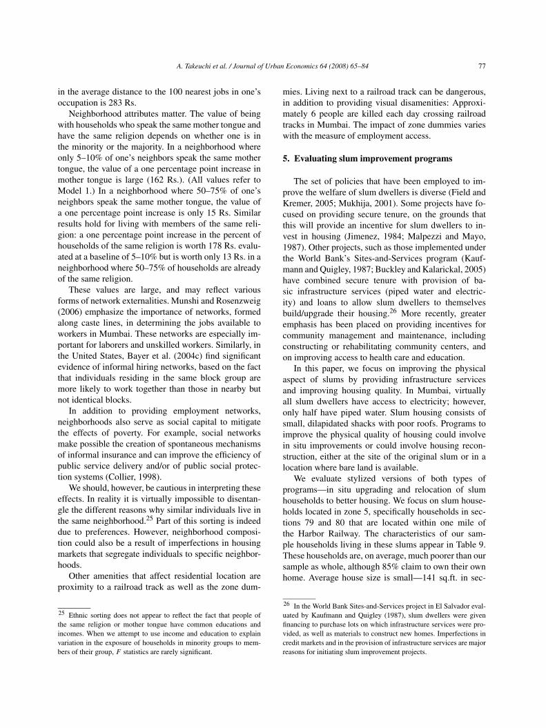
Figures 6 and 7 illustrate more clearly the impactof changes in neighborhood composition and employ-ment access on the benefits of slum improvement pro-grams. The figures plot the median CV associated withour sample improvement program, for all beneficiariesin Table 9, as the location of the improved housing ismoved to different places in the city. In Fig. 7 we assumethat the primary worker in the household maintains hiscurrent place of employment when the household re-locates; in Fig. 6 we measure employment opportuni-ties by the primary worker’s employment index. In bothfigures, lighter areas indicate locations that are welfare-reducing; darker areas indicate moves that are, on aver-age, welfare-enhancing. (In both figures, neighborhoodcomposition changes ipso facto with location.)


Fig. 6. CV for the relocation program using job access model.

When each worker’s job location is held fixed(Fig. 7), the set of locations for the program that yieldpositive benefits (positive mean CV) is small indeed.This has two important implications. It suggests that,in the short run, the net benefits of involuntary reset-tlement programs—even those that improve housingquality—could well be negative and might need to beaccompanied by cash transfers if they are not to reducewelfare. The second implication is that if potential par-ticipants in voluntary slum relocation programs lookonly at these programs from a short-run perspective(i.e., assuming that they cannot or will not change jobs),participation is likely to be low.

The set of locations yielding positive benefits ismuch larger in Fig. 6, in which household utility de-pends on the employment access index. A word of cau-

tion is, however, in order. The employment access indexdoes not capture spatial variation in wages, only varia-tion in proximity of jobs. The welfare measures in Fig. 6thus assume that earnings do not vary spatially. To ac-count for spatial variation in wages we estimated hedo-nic wage equations for the five occupational groups forwhich the employment access index is computed. Theaverage monthly wage for an unskilled male worker,who is married, 36 years old, has a high school degreeis approximately 3600 Rs. in zone 5. It is significantlylower than this only in zone 3, where it is 3000 Rs.per month. This suggests that the welfare gains froma program relocating households to sections 40–57 arelikely overstated. The general point made by comparingFigs. 6 and 7 is, however, clear: if workers can changejobs, the welfare improvements of relocation programs


Fig. 7. CV for the relocation program using distance to work model.

are greater, and the set of welfare-enhancing sites in-creases.

6. Conclusions

In order to design successful slum improvement pro-grams, it is important to determine whether programbenefits exceed program costs. It is also important, fromthe perspective of cost recovery, to determine householdwillingness to pay for specific program options. Theearly literature (Mayo and Gross, 1987) focused on es-timating the percent of income households were willingto spend on housing. This was followed by a literaturethat attempted to measure, using hedonic price func-tions, the market value of various improvements, includ-

ing tenure security and infrastructure services (Crane etal., 1997; Jimenez, 1984). It is, however, difficult us-ing the hedonic approach to value attributes that vary byhousehold, such as distance to work, or the percent ofneighbors similar to oneself. We believe that both setsof attributes are important in valuing slum improvementprograms and have attempted to extend the literatureby illustrating the value placed on these amenities byhouseholds in Mumbai.

We believe that the model estimated in this papercan be of use in calculating the relative welfare gainsfrom alternative slum improvement programs.29 It is

29 Unfortunately, comparing benefits with program costs is outsidethe scope of this paper.


also useful in predicting which households would belikely to participate in various programs, given costs ofparticipation. In assessing the limited success of sites-and-services programs, Mayo and Gross (1987) cite thefailure of many programs to choose the right packageof services to promote cost-recovery, a result echoed byBuckley and Kalarickal (2005). Location is an impor-tant component of the design of a slum improvementprogram. One contribution of this paper is to quantify,for the case of Mumbai, the quantitative importance oflocation versus other program characteristics. Anotheris to reinforce the results of other authors (Lall et al., inpress) who suggest that in situ improvements are, inmany cases, likely to dominate programs to relocateslum dwellers.

Acknowledgments

We thank Judy Baker, Rakhi Basu, and Somik Lall(The World Bank) for their contribution in data col-lection and the World Bank Research Committee andTransport Anchor (TUDTR) for funding the study. Wealso thank Pat Bayer and participants in seminars atJohns Hopkins University, NBER, and Stanford Univer-sity for their comments.

Table A.1Hedonic rent function estimates

Dependent var = ln(rent) 1 2

Slum −0.09 −0.09[4.34]*** [4.36]***

Coop 0.29 0.28[7.88]*** [7.78]***

Flat 0.34 0.34[9.28]*** [9 33]***

Good floor 0.06 0.06[2.55]** [2.63]***

Good wall 0.35 0.36[8.39]*** [8.44]***

Good roof 0.08 0.08[3.56]*** [3.33]***

Size 0.40 0.40[20.10]*** [20.18]***

Kitchen 0.06 0.07[2.91]*** [3.29]***

Toilet 0.10 0.10[3.80]*** [3.47]***

Bathroom 0.07 0.07[3 19]*** [3.16]***

Water 0.05 0.04[2.56]** [2.11]**

Table A.1 (continued)

Dependent var = ln(rent) 1 2

Near rail track −0.02 −0.03[1.22] [1.45]

zone = 2 −0.07 −0.08[1.60] [1.78]*

zone = 3 −0.13 −0.13[2.02]** [2.07]**

zone = 4 −0.22 −0.22[2.79]*** [2.80]***

zone = 5 −0.20 −0.20[3.26]*** [3.22]***

zone = 6 −0.25 −0.25[3.42]*** [3.41]***

Neighbor’s income 0.00004 0.00004[11.12]*** [10.88]***

Ln(distance to CBD) −0.09 −0.09[2.83]*** [2.66]***

Near rail station 0.00[0.10]

Near bus stop 0.14[4.86]***

Vehicle accessible road 0.04[1.80]*

Constant 4.56 4.38[38.46]*** [35.53]***

Observations 4132 4132Adjusted R2 0.639 0.641

Absolute value of t statistics in brackets.* Significant at 10%.

** Idem, 5%.*** Idem, 1%.

References

Baker, J., Basu, R., Cropper, M., Lall, S., Takeuchi, A., 2005. Urbanpoverty and transport: The case of Mumbai. Working paper #3683.Policy research, The World Bank.

Bayer, P., McMillan, R., Rueben, K.S., 2004a. What drives racial seg-regation? New evidence using census microdata. Journal of UrbanEconomics 56, 514–535.

Bayer, P., McMillan, R., Rueben, K.S., 2004b. An equilibrium modelof sorting in an urban housing market. Working paper #10865.NBER, Cambridge, MA.

Bayer, P., Ross, S., Topa, G., 2004c. Place of work and place of res-idence: Informal hiring networks and labor markets outcomes.Mimeo, Yale University.

Berry, S., 1994. Estimating discrete-choice models of product differ-entiation. RAND Journal of Economics 25, 242–262.

Berry, S., Levinsohn, J., Pakes, A., 1995. Automobile prices in marketequilibrium. Econometrica 63, 841–890.

Bertaud, A., 2004. Mumbai FSI conundrum: The perfect storm; thefour factors restricting the construction of new floor space inMumbai, Working paper. Available at http://alain-bertaud.com.

Buckley, R.M., Kalarickal, J., 2005. Housing policy in developingcountries: Conjectures and refutations. World Bank Research Ob-server 20 (2), 233–257.


Collier, P., 1998. Social capital and poverty. Working paper #4. SocialCapital Initiative, The World Bank.

Crane, R., Daniere, A., Harwood, S., 1997. The contribution of envi-ronmental amenities to low-income housing: A comparative studyof Bangkok and Jakarta. Urban Studies 34 (9), 1495–1512.

Field, E., Kremer, M., 2005. Impact evaluation for slum upgradinginterventions. Mimeo, Harvard University.

Ingram, G.K., Carroll, A., 1981. The spatial structure of Latin Amer-ican cities. Journal of Urban Economics 9 (2), 257–273.

Jimenez, E., 1984. Tenure security and urban squatting. Review ofEconomics and Statistics 66 (4), 556–567.

Kaufmann, D., Quigley, J.M., 1987. The consumption benefits of in-vestment in infrastructure: The evaluation of sites-and-servicesprograms in underdeveloped countries. Journal of DevelopmentEconomics 25 (2), 263–284.

Lall, S., Lundberg, M., Shalizi, Z., in press. Implications of alternatepolicies on welfare of slum dwellers: Evidence from Pune, India.Journal of Urban Economics.

McFadden, D., 1978. Modeling the choice of residential location. In:Karlqvist, A., Lundquist, L., Snickars, F., Weibull, J. (Eds.), Spa-tial Interaction Theory and Planning Models. Amsterdam, North-Holland.

Malpezzi, S., Mayo, S.K., 1987. User cost and housing tenure in de-veloping countries. Journal of Development Economics 25, 197–220.

Mayo, S.K., Gross, D.J., 1987. Sites and services—And subsidies:The economics of low-cost housing in developing countries.World Bank Economic Review 1, 301–335.

Mohan, R., 1994. Understanding the Developing Country Metropo-lis: Lessons from the City Study of Bogota and Cali, Colombia.Oxford Univ. Press.

Mukhija, V., 2001. Upgrading housing settlements in developingcountries: The impact of existing physical conditions. Cities 18(4), 213–222.

Mukhija, V., 2002. An analytical framework for urban upgrading:Property rights, property values and physical attributes. HabitatInternational 26, 553–570.

Munshi, K., Rosenzweig, M., 2006. Traditional institutions meet themodern world: Caste, gender and schooling choice in a globalizingeconomy. American Economic Review 96 (4), 1225–1252.

Sclar, E.D., Garau, P., Carolini, G., 2005. The 21st century healthchallenge of slums and cities. Lancet 365, 901–903.

Takeuchi, A., Cropper, M., Bento, A., 2007. The impact of policiesto control motor vehicle emissions in Mumbai, India. Journal ofRegional Science 47 (1), 27–46.

United Nations Global Report on Human Settlements, 2003. Thechallenge of slums. United Nations Human Settlements Program.Earthcan Publications Ltd., London, UK.

Measuring the welfare effects of slum improvement programs ... · Measuring the welfare effects of...

Documents

Transcript of Measuring the welfare effects of slum improvement programs ... · Measuring the welfare effects of...