Crawford School of Public Policy

CAMA Centre for Applied Macroeconomic Analysis

Measuring the stance of monetary policy in conventional and unconventional environments

CAMA Working Paper 6/2014 January 2014 Leo Krippner Reserve Bank of New Zealand and Centre for Applied Macroeconomic Analysis Abstract

This article introduces an idea for summarizing of the stance of monetary policy with quantities derived from a class of yield curve models that respect the zero lower bound constraint for interest rates. The “economic stimulus measure” aggregates the current and estimated expected path of interest rates relative to the neutral interest rate from the yield curve model. Unlike shadow short rates, economic stimulus measures are consistent and comparable across conventional and unconventional monetary policy environments, and are less subject to variation with modelling choices, as I demonstrate with two and three factor models estimated with different data sets. Full empirical testing of the inter-relationships between ES measures and macroeconomic data remains a topic for future work.

T H E A U S T R A L I A N N A T I O N A L U N I V E R S I T Y

Keywords Unconventional monetary policy; zero lower bound; shadow short rate; term structure model JEL Classification E43, E52, G12 Address for correspondence: (E) cama.admin@anu.edu.au

The Centre for Applied Macroeconomic Analysis in the Crawford School of Public Policy has been established to build strong links between professional macroeconomists. It provides a forum for quality macroeconomic research and discussion of policy issues between academia, government and the private sector. The Crawford School of Public Policy is the Australian National University’s public policy school, serving and influencing Australia, Asia and the Pacific through advanced policy research, graduate and executive education, and policy impact.

T H E A U S T R A L I A N N A T I O N A L U N I V E R S I T Y

Measuring the stance of monetary policy inconventional and unconventional environments

Leo Krippner∗

17 December 2013

Abstract

This article introduces an idea for summarizing of the stance of monetary pol-icy with quantities derived from a class of yield curve models that respect the zerolower bound constraint for interest rates. The “economic stimulus measure” ag-gregates the current and estimated expected path of interest rates relative to theneutral interest rate from the yield curve model. Unlike shadow short rates, eco-nomic stimulus measures are consistent and comparable across conventional and un-conventional monetary policy environments, and are less subject to variation withmodeling choices, as I demonstrate with two and three factor models estimatedwith different data sets. Full empirical testing of the inter-relationships between ESmeasures and macroeconomic data remains a topic for future work.JEL: E43, E52, G12Keywords: unconventional monetary policy; zero lower bound; shadow short

rate; term structure model

1 Introduction

This article proposes a new measure of the stance of monetary policy derived fromshadow/zero lower bound (ZLB) yield curve models. The motivation for what I callthe “economic stimulus measure”(ES measure) is to improve on aspects that have beenquestioned regarding the use of shadow short rates (SSRs) as a summary metric for thestance of unconventional monetary policy. The ES measure also offers improvements onan alternative metric, i.e. the horizon to non-zero policy rates.As background, SSRs obtained from shadow/ZLB yield curve models have been pro-

posed as a measure of the stance of monetary policy in Krippner (2011, 2012, 2013b,d)as cited by Bullard (2012, 2013), and Wu and Xia (2013) as cited by Hamilton (2013)and Higgins and Meyer (2013) The proposal has intuitive appeal because when the SSRis positive it equals the actual short rate, but the SSR is free to evolve to negative lev-els after the actual short rate becomes constrained by the ZLB. Figure 1 illustrates theconcept for the U.S. Federal Funds Rate (FFR) and an estimated shadow short rate fromDecember 2008, when the FFR was set to a 0-0.25% target range. In essence, the SSR

∗Reserve Bank of New Zealand and Centre for Applied Macroeconomic Analysis. Email:leo.krippner@rbnz.govt.nz. I thank Iris Claus, Edda Claus, and Fernando Yu for helpful comments.

1

evolves like the short rate that would prevail in the absence of physical currency,1 and soit can be used as an indicator of further policy easing beyond the zero policy rate. Quan-titatively, comparing the unconventional/ZLB and conventional/pre-ZLB periods for theU.S., Claus, Claus, and Krippner (2013) show that the SSR responds to monetary policyshocks similarly to the FFR, and Wu and Xia (2013) show that the effects of the SSR onmacroeconomic variables are similar to the FFR.

Figure 1: The Federal Funds Rate (FFR) and the estimated shadow short rate (SSR) fromDecember 2008. The ZLB constrains the FFR essentially at zero, while the SSR can freely

evolve to negative levels.

Nevertheless, negative SSRs are necessarily estimated quantities, and so they willvary with the practical choices underlying their estimation. In particular, it has beenwell-established in Christensen and Rudebusch (2013a,b), Bauer and Rudebusch (2013),and Krippner (2013d) that SSR estimates can be materially sensitive to the followingchoices: (1) the specification of the shadow/ZLB model (e.g. Black (1995) or Krippner(2012, 2013), two or three factors, parameter restrictions on the mean-reversion matrix,etc.); (2) the data used for estimation (e.g. using yield curve data out to maturities of 10year or 30 years, and the sample period); and (3) the method used for estimation (e.g.the extended, iterated extended, or the unscented Kalman filters).2

In addition, from an economic perspective, negative shadow rates are not an actualinterest rate faced by economic agents. That is, borrowers face current and expectedinterest rates that are based on the ZLB constraint (with appropriate margins), not neg-ative interest rates (which would result in borrowers being paid the absolute interestrate by investors). As such, SSRs are not consistent and directly comparable acrossconventional/non-ZLB and unconventional/ZLB environments. To highlight this point,figure 2 illustrates that easing the SSR from 5 to 0 percent provides more monetary policy

1Physical currency effectively sets the ZLB for interest rates because it is always available as analternative investment to bonds, but with a zero rate of return.

2Longer maturity spans and estimation with the iterated extended Kalman filter produce more negativeSSR estimates; see Krippner (2013d).

2

stimulus than easing the SSR from 0 to -5 percent, because the entire yield curve movesdown markedly in first case but the ZLB constrains declines in short- and mid-maturityinterest rates in the second case.3

0 5 10

­5

0

5

ZLB and shadow  yield curv e examples

Time to maturi ty

Perc

enta

ge p

oint

s

SSR = 5%SSR = 0%SSR = ­5%

Figure 2: ZLB yield curves and shadow yield curves (dotted lines below ZLB yield curves) fordifferent values of the SSR, while keeping the long-run yields constant. Monetary policy

stimulus from the ZLB yield curve (i.e. declines in actual interest rates) is attenuated whenthe SSR adopts negative values.

As an alternative metric for unconventional monetary policy, Bauer and Rudebusch(2013) propose the “lift-offhorizon”, i.e. the median time for simulated future actual shortrates from the estimated shadow/ZLB model to reach 0.25 percent. The lift-off horizonhas proven more robust than the SSR to different model specifications, and it also providesa probabilistic summary measure of actual interest rates faced by economic agents for thegiven horizon, rather than the non-obtainable and therefore less economically relevantnegative SSRs. However, the lift-off horizon does not provide an indication of whateconomic agents will face for longer horizons into the future, which should also influencetheir decisions, and neither does it have a conventional counterpart for comparison acrossnon-ZLB and ZLB environments.The ES measure that I propose improves on the SSR and the lift-offhorizon by directly

summarizing current and expected actual interest rates relative to the neutral interest rate.Specifically, I obtain the expected path of the actual short rate and its long-run expec-tation from a shadow/ZLB Gaussian affi ne term structure model (hereafter GATSM) ofthe yield curve and then integrate the difference between those quantities over the hori-zon from zero to infinity. In ZLB periods, short rate expectations will initially include aperiod of zero followed by an non-zero path that converges to the long-run expectation,and in non-ZLB periods the expected path of the short rate is entirely non-zero as itconverges to the long-run expectation. However, in both regimes, the ES measure aggre-gates expected short rates relative to their long-run expectation from the same estimated

3Figure 9 latter provides a more detailed perspective on how monetary policy stimulus attentuates asa function of the SSR.

3

model, and so the ES measure is directly comparable between ZLB and non-ZLB periods.The practical advantage of ES measures is their robustness relative to SSRs; i.e. theES measures obtained from shadow/ZLB-GATSMs with two and three factors estimatedwith different data turn out to be very similar, while the corresponding SSR estimatesare quite different.The article proceeds as follows. Section 2 provides an overview of the Krippner (2011,

2012, 2013) and Black (1995) shadow/ZLB-GATSMs, respectively the K-GATSM andB-GATSM hereafter.4 In section 3, I first outline how ES measures may be obtainedusing the shadow-GATSM from either the K-GATSM or B-GATSM, and then apply theES framework to the K-GATSM results under the risk-adjusted measure from Krippner(2013d). Section 4 introduces and illustrates ES measures under the physical measure.Section 5 discusses some ideas related to the ES measure to follow up in future work,including potential improvements, empirical testing, and some conceptual questions. Sec-tion 6 concludes.

2 Overview of shadow/ZLB-GATSMs

In this section, I provide an overview of the K-GATSM and B-GATSM classes of models.The main objective from the perspective of the present article is to establish notationfor the shadow-GATSM, which contains the component subsequently used to define theES measures in sections 3 and 5. I also briefly discuss in section 2.2 how the modelsmay be estimated in principle so it is apparent how observed yield curve data and thespecified model defines the ES measures. Details and examples of actual estimations areavailable from the given references; in this article I simply use the results already availablefrom Krippner (2013d) and some supplementary estimations to illustrate ES measures inpractice.

2.1 The shadow-GATSM term structure

I adopt the generic GATSM specification from Dai and Singleton (2002) pp. 437-38 todefine the shadow-GATSM. Hence, the SSR is:

r (t) = a0 + b′0 x (t) (1)

where a0 is a constant, b0 is a constant N×1 vector containing the weights for the N statevariables xn (t), and x (t) is an N×1 vector containing the N state variables xn (t). Underthe physical Pmeasure, x (t) evolves as the following correlated vector Ornstein-Uhlenbeckprocess:

dx (t) = κ [θ − x (t)] dt+ σdW (t) (2)

where θ is a constant N × 1 vector representing the long-run level of x (t), κ is a constantN ×N matrix that governs the deterministic mean reversion of x (t) to θ, σ is a constantN ×N matrix representing the potentially correlated volatilities of x (t), and dW (t) is anN ×1 vector with independent Wiener components dWn (t) ∼ N (0, 1)

√dt. From Meucci

(2010) p. 3, the solution for the stochastic differential equation is:

x (t+ τ) = θ + exp (−κτ) [x (t)− θ] +

∫ t+τ

t

exp (−κ [τ − u])σdW (u) (3)

4The Wu and Xia (2013) model is a discrete-time version of the K-GATSM, although it is deriveddifferently.

4

which gives the following expectation, as at time t, under the P measure (also see Dai andSingleton (2002) p. 438):

Et [x (t+ τ)] = θ + exp (−κτ) [x (t)− θ] (4)

Therefore, what I will call the expected path of the SSR under the Pmeasure, Et [r (t+ τ)],is:

Et [r (t+ τ)] = a0 + b′0Et [x (t+ τ)]

= a0 + b′0 {θ + exp (−κτ) [x (t)− θ]} (5)

Note that the current SSR, r(t), is contained in Et [r (t+ τ)], i.e.:

Et [r (t+ τ)]|τ=0 = a0 + b′0x (t) = r (t) (6)

and so the current and expected SSRs do not need to be referred to separately (whichalso holds for Et [r (t+ τ)] below).The market prices of risk are linear with respect to the state variables, i.e.:5

Π (t) = σ−1 [γ + Γx (t)] (7)

where γ and Γ are respectively a constant N × 1 vector and constant N ×N matrix. Therisk-adjusted process for x (t) is:

dx (t) = κ[θ − x (t)

]dt+ σdW (t) (8)

where κ = κ+ Γ and θ = κ−1 (κθ − γ).Shadow forward rates for the shadow-GATSM are:

f (t, τ) = Et [r (t+ τ)] +VE (τ) (9)

where Et [r (t+ τ)] is the expected path of the SSR under the risk-adjusted Q measure:

Et [r (t+ τ)] = a0 + b′0

{θ + exp (−κτ)

[x (t)− θ

]}(10)

and VE(τ) is the forward rate volatility effect from Krippner (2013d) appendix I:

VE (τ) =1

2

[∫ τ

0

b′0 exp (−κτ) ds]σσ′

[∫ τ

0

exp (−κ′τ) b0 ds]

(11)

The expression for shadow interest rates R(t, τ) is defined using the standard continuous-time term structure relationships,6 i.e.:

R (t, τ) =1

τ

∫ τ

0

f (t, u) du (12)

5This is the “essentially affi ne”specification from Duffee (2002), but for a model with full Gaussiandynamics. Also see Cheridito, Filipovic, and Kimmel (2007) for further discussion on market price of riskspecifications.

6References for this standard term structure relationship and others I use subsequently in the articleare, for example, Filipovic (2009) p. 7 or James and Webber (2000) chapter 3.

5

2.2 ZLB-GATSM term structures and estimation

K-GATSM forward rates are defined as (see Krippner (2013d) p. 16):

f¯

(t, τ) = f (t, τ) · Φ[f (t, τ)

ω (τ)

]+ ω (τ) · 1√

2πexp

(−1

2

[f (t, τ)

ω (τ)

]2)(13)

and R¯

(t, τ) is obtained using the standard term structure relationship:

R¯

(t, τ) =1

τ

∫ τ

0

f¯

(t, u) du (14)

which is straightforward to evaluate with univariate numerical integration over time tomaturity τ . The K-GATSM has already been established as an empirically acceptableapproximation to the B-GATSM (which imposes the ZLB in a fully arbitrage-free way),but the relative tractability of the K-GATSMmakes it much quicker to apply; see Krippner(2013d), Christensen and Rudebusch (2013a,b), and Wu and Xia (2013).Black-GATSM bond prices may be defined generically as (see Krippner (2013d) p. 6):

P¯B (t, τ) = Et

{exp

(−∫ τ

0

max {0, r (t+ u)} du)}

(15)

and R¯B (t, τ) is obtained using the standard term structure relationship:

R¯B (t, τ) = −1

τlogP

¯B (t, τ) (16)

In practice, interest rates for multifactor B-GATSM implementations have been obtainedusing the multivariate numerical methods of finite-difference grids, interest rate lattices,and Monte Carlo simulations; e.g. see Bomfim (2003), Ueno, Baba, and Sakurai (2006),Ichiue and Ueno (2007), Kim and Singleton (2012), Ichiue and Ueno (2013), Bauer andRudebusch (2013), and Richard (2013).7 Recent advances in Priebsch (2013) and Krippner(2013a) offer faster B-GATSM implementations, respectively via a close second-order ap-proximation, and Monte Carlo simulation with a control variate based on the K-GATSM.Regarding estimation, the state equation for both the K-GATSM and B-GATSM is:

xt+1 = θ + exp (−κ∆t) (xt − θ) + εt+1 (17)

where∆t is the time increment between observations, the subscript t is an integer index forthe time series of term structure observations, and εt+1 is the N × 1 vector of innovationsto the state variables. The measurement equation for both the K-GATSM and B-GATSMis:

R¯ t

= R¯

(xt,A) + ηt (18)

where R¯ tis the K × 1 vector of interest rate data at time index t, R

¯(xt,A) is the K × 1

vector of shadow/ZLB-GATSM rates with A denoting the parameters already noted in7Gorovoi and Linetsky (2004) develops a semi-analytic solution for one factor B-GATSMs, which has

been applied in Ichiue and Ueno (2006) and Ueno, Baba, and Sakurai (2006).

6

section 2.1, and ηt is the K × 1 vector of components unexplained by the shadow/ZLB-GATSM.8 The K-GATSM uses interest rates defined by equation 14 in equation 18, whilethe B-GATSM uses interest rates defined by equation 16 in equation 18.The state space representation has been estimated with the extended, iterated ex-

tended, or unscented Kalman filters (e.g. see Kim and Singleton (2012), Krippner (2013d),and Kim and Priebsch (2013) respectively). Christensen and Rudebusch (2013a, b),Krippner (2013d), and Wu and Xia (2013) adopt a common normalization for identifica-tion and estimation, which I assume hereafter, of fixed values for b0, diagonal blocks ofreal Jordan matrices for κ (which allows for repeated eigenvalues), θ = 0, and a lowerdiagonal matrix σ.9 As detailed in section 3.1, when one eigenvalue of κ and/or κ is setto zero, the further restriction a0 = 0 applies.

3 ES measures from shadow/ZLB-GATSMs

In this section, I first show how the expected path of the SSR and its long-run expectation(which I interpret as the neutral interest rate) under the risk-adjusted Q measure can beused to create what I will call the ES-Q measure. I use a specification where the non-stationary restriction κ1 = 0 is imposed on the first eigenvalue because that results in themost intuitive and parsimonious framework, as I subsequently illustrate in sections 3.2and 3.3. In section 3.4, I show that the K-AFNSM ES-Q measures are empirically morerobust to different specifications and data sets than SSR estimates, and discuss why ES-Qmeasures should in principle be superior to alternative indicators of the monetary policystance. Section 3.5 compares ES-Q measures in more detail.ES-Q measures can be similarly derived if stationary GATSMs (i.e. where all eigen-

values κi of κ for the shadow GATSM are greater than zero) are used to represent theshadow term structure. However, the interpretation of stationary GATSMs is more in-volved without adding anything to the principles of the ES-Q measures for non-stationaryGATSMs, so I relegate those details and illustrations to appendix A.

3.1 ES-Q measure with κ1 = 0

With the block-diagonal specification and κ1 = 0, x1 (t) becomes a Level state variablethat follows a random walk. Therefore, the parameter a0 is restricted to zero, becauseit can no longer be identified in the estimation, and because it is redundant from aneconomic perspective given that x1 (t) completely captures the long-run expectation of

8The Wu and Xia (2013) K-GATSM is estimated using forward one-month rates constructed fromthe estimated Svensson (1995)/Nelson and Siegel (1987) model parameters reported in Gürkaynak, Sack,and Wright (2007). Continuous-time K-GATSMs could be estimated analogously using instantaneousforward rates constructed from the same data set. However, I prefer to use an interest rate measurementequation with interest rate data because that is standard in the literature, and forward rate data are notavailable or readily obtainable for interest rate data sets generated from non-parametric methods; e.g.Bloomberg data (see Kushnir (2009) for method details) and Fama and Bliss (1987).

9Different normalizations could be chosen, such as a lower diagonal κ matrix and a diagonal σ matrix,or θ = 0 with θ estimated, but they would be observationally equivalent representations of the yieldcurve data. Appendix B shows how non-block-diagonal specifications may be handled, effectively bypre-diagonalizing the original specification.

7

Et [r (t+ τ)]. Specifically, the expected path of the SSR is:

Et [r (t+ τ)] = b′0 exp (−κτ)x (t)

=[b0,1, b

′0,L

]exp

(−[

0 00 κL

]τ

)[x1 (t)xL (t)

]=

[b0,1, b

′0,L

] [ 1 00 exp (−κLτ)

] [x1 (t)xL (t)

]= b0,1x1 (t) + b′0,L exp (−κLτ)xL (t) (19)

where b0,L is the (N − 1)× 1 lower-block vector of b0, κL is the (N − 1)× (N − 1) lower-block matrix of κ, and xL (t) is the (N − 1) × 1 lower-block vector of x (t). The SSRis:

Et [r (t+ τ)]∣∣∣τ=0

= b′0x (t) = r (t) (20)

and the long-run expectation/neutral rate is:

limτ→∞

Et [r (t+ τ)] = b0,1x1 (t) (21)

A common example of this specification in GATSMs is the three-factor arbitrage-free Nelson and Siegel (1987) model, or hereafter AFNSM(3); e.g. see Krippner (2006),Christensen, Diebold, and Rudebusch (2011), and Diebold and Rudebusch (2013). In thatcase, the remaining two eigenvalues are restricted to be equal, i.e. κ2 = κ3 > 0. However,the following expressions would also apply if κ2 and κ3 were allowed to be distinct, orif just one non-Level factor were used, as with the AFNSM(2) used to represent theshadow term structure in section 3.2. Empirically, the restriction κ1 = 0 can generallybe imposed for parsimony because estimated GATSMs and shadow/ZLB-GATSMs withκi > 0 inevitably turn out to have one eigenvalue κ1 & 0.10

I define the ES-Q measure at time t, denoted ξ (t), as the integral of the expected pathof the shadow short rate truncated at zero relative to its long-run value, i.e.:

ξ (t) =

∫ ∞0

(b0,1x1 (t)−max

{0, Et [r (t+ τ)]

})dτ

=

∫ ∞0

(max

{b0,1x1 (t) , b0,1x1 (t)− b0,1x1 (t)− b′0,L exp (−κLτ)xL (t)

})dτ

=

∫ ∞0

(max

{b0,1x1 (t) ,−b′0,L exp (−κLτ)xL (t)

})dτ (22)

As I will subsequently explain in section 5.2, I intentionally use max{

0, Et [r (t+ τ)]}

to define ξ (t), rather than using the non-equivalent alternative Et [max {0, r (t+ τ)}]. Thelatter would result in infinite ES-Q measures, which would not correlate empirically withmacroeconomic variables and would therefore not be a useful quantity in practice.

3.2 K-AFNSM(2) ES-Q measure

The ES-Q measure in practice is most clearly illustrated for the two-factor K-AFNSM,or K-AFNSM(2) hereafter. The parsimony of the AFNSM(2) when representing the

10See, for example, Kim and Singleton (2012) and Ichiue and Ueno (2013) for B-GATSMs, and Wu andXia (2013) for a K-GATSM example. Krippner (2013c) provides a wide range of results for GATSMs.

8

shadow term structure makes it very convenient mathematically, and the AFNSM(2)is also realistic from a macro-finance perspective for the following four reasons: (1) itcontains the Level and Slope components of the term structure, which proxy the firsttwo principal components that in turn explain 99.9 percent of variation in the GSW10and GSW30 data sets; (2) it approximates the generic GATSM (hence, any GATSM thatcould be specified) to first order in the sense discussed in Krippner (2013c);11 (3) theLevel and Slope have been shown to relate respectively to inflation and output growth(see Krippner (2008) for discussion of the principles and Diebold, Rudebusch, and Aruoba(2006) for empirical evidence); and (4) related to the previous point, the Level componentis modelled as a unit root process. The latter corresponds with empirical evidence thatinflation is a strongly persistent process where a unit root typically cannot be rejected;e.g. see Aïssa and Jouini (2003).For the K-AFNSM(2), Et [r (t+ τ)] is defined with b′0 = [1, 1], and a mean-reversion

matrix κ with zeros apart from φ in the lower diagonal element. Hence, equation 19becomes:

Et [r (t+ τ)] = x1 (t) + x2 (t) · exp (−φτ) (23)

with the SSR:r (t) = x1 (t) + x2 (t) (24)

and the long-run expectation:

limτ→∞

Et [r (t+ τ)] = x1 (t) (25)

Rather than immediately deriving a general analytic expression for ξ (t) at this stage,it is more insightful to illustrate the ES-Q measure graphically, and so figures 3 and 4provide examples of the two cases that can occur in practice.12 Note that, unless statedotherwise, all figures in section 3 are based on the K-AFNSM(2) and K-AFNSM(3) modelsfrom Krippner (2013d) which are estimated (with the iterated extended Kalman filter)using month-end Gürkaynak, Sack, andWright (2007) yield curve data with maturities outto 30 years (hereafter the GSW30 data set). Specifically, the maturities of the GSW30data set are 0.25, 0.5, 1, 2, 3, 4, 5, 7, 10, 15, 20, and 30 years, the sample period isNovember 1985 (the first month from which 30 year data were available) to July 2013(the last month available at the time of the Krippner (2013d) estimations). I also useresults estimated with GSW10 data (i.e. the GSW30 data set without the last threeyields), but the GSW30 data should in principle provide better estimates of the Levelstate variable and hence the ES-Q measure, and section 3.4 shows that is indeed the casein practice. Note also that the principles of the illustrations also apply to B-GATSMs,but the estimates of the shadow-GATSM parameters and state variables from the datawould differ somewhat.11Krippner (2013c) sets the near-zero eigenvalues of the mean-reversion matrix κ for the generic GATSM

equal to zero and the non-persistent eigenvalues to their mean value denoted as φ. The components of thegeneric GATSM then condense to the AFNSM(2). The extension to the AFNSM(3) allows an additionalterm in the Taylor expansion for the non-persistent eigenvalues around φ, which results in the additionof the Bow component relative to the AFNSM(2).12Other possibilities with x1 (t) < 0 are purely mathematical; such estimates do not arise in practice,

and a negative neutral interest rate would lack an economic interpretation in any case.

9

Figure 3: U.S. yield curve data, estimated K-AFNSM(2) results, and the ES-Q measure forJuly 2011. This example illustrates the case for a negative SSR, which in turn corresponds to

an unconventional/ZLB monetary policy environment.

Figure 3 illustrates ξ (t) as the shaded region for an unconventional/ZLB environment.This example is as at July 2011, and I use that date often throughout the article todemonstrate alternative models. For figure 3, the estimated Level and Slope state variablesare x1 (t) = 5.70% and x2 (t) = −12.62%, giving an SSR of r(t) = −6.91%, which means

the truncation max{

0, Et [r (t+ τ)]}will bind for future horizons τ ∈ [0, τ 0]. The value

of τ 0 is obtained by setting Et [r (t+ τ 0)] = x1 (t) + x2 (t) · exp (−φτ 0) = 0 and solving forτ 0, with the result:

τ 0 = −1

φlog

[−x1 (t)

x2 (t)

](26)

which has a value of τ 0 = 2.32 years in figure 3, given the parameter estimate φ = 0.3196.In general, ξ (t) will have two components when r(t) < 0. Specifically, equation 22

with b0,L = 1 and κL = φ gives:

ξ (t) =

∫ ∞0

(max {x1 (t) ,−x2 (t) · exp (−κτ)}) dτ

=

∫ τ0

0

x1 (t) dτ −∫ ∞τ0

x2 (t) · exp (−φτ) dτ (27)

10

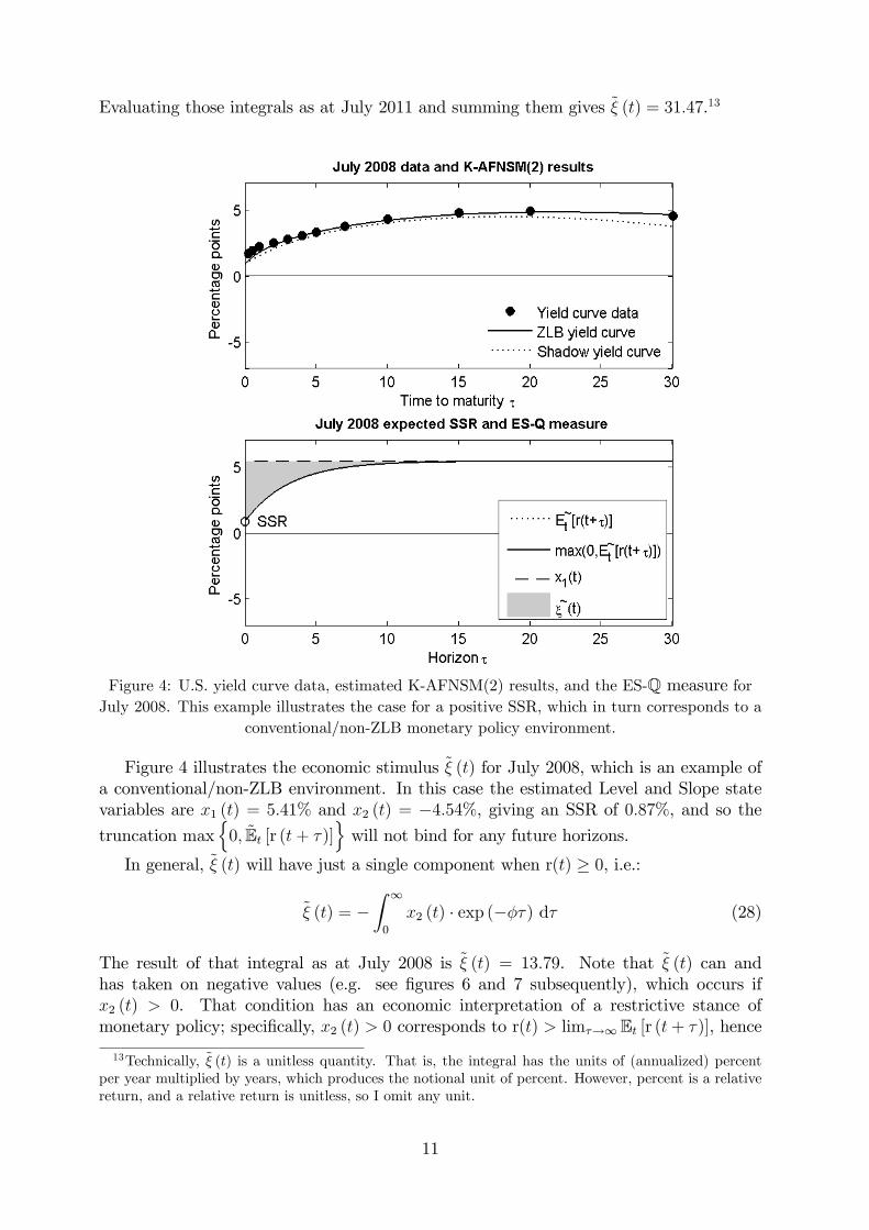
Evaluating those integrals as at July 2011 and summing them gives ξ (t) = 31.47.13

Figure 4: U.S. yield curve data, estimated K-AFNSM(2) results, and the ES-Q measure forJuly 2008. This example illustrates the case for a positive SSR, which in turn corresponds to a

conventional/non-ZLB monetary policy environment.

Figure 4 illustrates the economic stimulus ξ (t) for July 2008, which is an example ofa conventional/non-ZLB environment. In this case the estimated Level and Slope statevariables are x1 (t) = 5.41% and x2 (t) = −4.54%, giving an SSR of 0.87%, and so the

truncation max{

0, Et [r (t+ τ)]}will not bind for any future horizons.

In general, ξ (t) will have just a single component when r(t) ≥ 0, i.e.:

ξ (t) = −∫ ∞0

x2 (t) · exp (−φτ) dτ (28)

The result of that integral as at July 2008 is ξ (t) = 13.79. Note that ξ (t) can andhas taken on negative values (e.g. see figures 6 and 7 subsequently), which occurs ifx2 (t) > 0. That condition has an economic interpretation of a restrictive stance ofmonetary policy; specifically, x2 (t) > 0 corresponds to r(t) > limτ→∞ Et [r (t+ τ)], hence

13Technically, ξ (t) is a unitless quantity. That is, the integral has the units of (annualized) percentper year multiplied by years, which produces the notional unit of percent. However, percent is a relativereturn, and a relative return is unitless, so I omit any unit.

11

r¯(t)− limτ→∞ Et [r (t+ τ)] > 0, which in turn implies that the current actual interest ratesare restrictive relative to their neutral interest rate.Summarizing the two cases, the general analytic expression ξ (t) with the AFNSM(2)

is therefore:

ξ (t) =

∫ τ00x1 (t) dτ −

∫∞τ0x2 (t) · exp (−φτ) dτ if r (t) < 0

−∫∞0x2 (t) · exp (−φτ) dτ if r (t) ≥ 0

(29)

3.3 K-AFNSM(3) ES measure

For the K-AFNSM(3), Et [r (t+ τ)] is defined with b′0 = [1, 1, 0] and a mean-reversionmatrix κ with zeros apart from the following lower diagonal Jordan block:

κL =

[φ −φ0 φ

](30)

Hence, equation 19 becomes:

Et [r (t+ τ)] = x1 (t) + x2 (t) · exp (−φτ) + x3 (t) · φτ exp (−φτ) (31)

which is the AFNSM(2) expression with the addition of a Bow component, i.e. x3 (t) ·φτ exp (−φτ),14 that improves the fit of mid-maturity rates. The expressions for thelong-run expectation and the SSR are the same as for the K-AFNSM(2).In principle, the general analytic expression for ξ (t) from the AFNSM(3) would involve

the two cases for the AFNSM(2) and an additional potential case where Et [r (t+ τ)] < 0for intermediate values of τ (i.e. 0 < τ 1 < τ < τ 2). However, the latter case has neveroccurred in practice, and so the ξ (t) general analytic expression for the AFNSM(3) isanalogous to the AFNSM(2) with the addition of the Bow component, i.e.:

ξ (t) =

∫ τ00x1 (t) dτ −

∫∞τ0x2 (t) · exp (−φτ) + x3 (t) · φτ exp (−φτ) dτ if r (t) < 0

−∫∞0x2 (t) · exp (−φτ) + x3 (t) · φτ exp (−φτ) dτ if r (t) ≥ 0

(32)where τ 0 is readily found numerically (e.g. using the “fzero”function in MatLab) as thesolution to Et [r (t+ τ 0)] = x1 (t) +x2 (t) · exp (−φτ 0) +x3 (t) ·φτ exp (−φτ) = 0. In figure5, τ 0 = 2.38 years, which compares to τ 0 = 2.32 years for the AFNSM(2).Figure 5 illustrates ξ (t) for the AFNSM(3) as at July 2011. In this case the estimated

Level, Slope, and Bow state variables of x1 (t) = 6.11%, x2 (t) = −8.82%, and x3 (t) =−8.46% give ξ (t) = 33.87, which is close to the value of ξ (t) = 31.47 for the K-AFNSM(2)in figure 3. However, the SSR of r(t) = −2.71% is distinctly different from the value of−6.91% for the AFNSM(2) in figure 3, which in turn arises from the influence of the Bowcomponent in fitting the observed yield curve data.

14See Diebold and Rudebusch (2013) for further discussion on Nelson and Siegel (1987) models andAFNSMs. My preferred name “Bow” is often referred to as “Curvature” in that book and the relatedliterature. However, the Slope component itself has a natural curvature, resulting from its exponentialdecay functional form, so Bow is a less ambiguous (and syllable-saving) name for the third AFNSMcomponent.

12

Figure 5: U.S. yield curve data, estimated K-AFNSM(3) results, and the ES-Q measure forJuly 2011. This example illustrates an alternative estimate for the unconventional/ZLB

monetary policy environment illustrated in figure 3. The resulting ES measure is similar tofigure 3, while the SSR is distinctly different.

3.4 Comparing K-AFNSM ES measures to SSRs

3.4.1 Empirical perspective

Figure 6 plots the time series of the ES-Q measures and the SSRs for the K-AFNSM(2)and K-AFNSM(3) results obtained with the GSW30 data set, and figure 7 plots the resultsobtained with the GSW10 data set. Note that I have indicated NBER recessions withthe shaded areas, as I will do for all full-sample time series figures, to provide a verypreliminary gauge on how the series relate to real output growth. Section 5.1 discussesthe more systematic analysis that would obviously be required to fully assess the practicaluse of ES-Q measures.One key point from the time series figures is that, within and across both figures,

the ES-Q measures are much closer to each other than the SSR estimates. This resultsuggests that the ES-Q measures are more robust than SSRs with respect to the numberof factors used to specify the model and the data used for estimation. That said, there isstill some variation between the ES-Q measures, particularly a notable divergence at theend of the sample, which warrants further discussion in section 3.5.

13

Figure 6: Time series plots of the ES-Q measures and the SSRs for the K-AFNSM(2) andK-AFNSM(3) estimated with GSW30 data. The ES-Q measures are more robust across the

estimated models than the SSR estimates.

Another key point from figures 6 and 7 is that ES-Q measures appear to correlate wellwith output growth. Specifically, the periods where the ES-Qmeasures are high follow theonset of NBER recessions, and the larger recession associated with the Global FinancialCrisis is followed with a more extreme and prolonged ES-Q measure than the previoustwo recessions. The higher ES-Q measures are in turn consistent with easier monetarypolicy to close the output gaps that arise in the wake of the recessions. In that regard, theSSR estimates have a complementary profile, but with wider variation between differentmodel estimates as previously mentioned.

3.4.2 Theoretical perspective

To highlight the economic interpretation of the ES-Q measures, note that they changecontinuously with the changing shape of the yield curve, which in turn implies: (1) achange to the expected path of the SSR; and/or (2) a change to the long-run SSR expec-tation, which is used as a proxy for the neutral interest rate (and both are coincident withthe long-run expectation of the actual short rate). I discuss each of the two componentsin turn.

14

Figure 7: Time series plots of the ES-Q measures and the SSRs for the K-AFNSM(2) andK-AFNSM(3) estimated with GSW10 data. The ES-Q measures are more robust across the

estimated models than the SSR estimates.

In non-ZLB periods, the expected path of the SSR can change independently of changesto the policy rate, which is appropriate because even conventional monetary policy op-erates partly through signalling and expectations; e.g. see Walsh (2003) chapter 10 fordiscussion of the principles and Gürkaynak, Sack, and Swanson (2005) for empirical evi-dence. In ZLB periods, forward guidance and expectations are an important componentof unconventional monetary policy; e.g. see Woodford (2012) section 1. Note, however,that Et [r (t+ τ)] can and does change beyond the direct influence of either conventionalor unconventional monetary policy actions, essentially by any factors that influence theyield curve. Therefore, Et [r (t+ τ)] and ES-Q measures should be treated as market ex-pectations variables subject to central bank influence, rather than quantities explicitlycontrolled by the central bank like the FFR or asset purchase programs. In that respect,Et [r (t+ τ)] is similar to the lift-off horizon, which can be influenced but not explicitlycontrolled by the central bank.Regarding the long-run SSR expectation/neutral interest rate, it can change to reflect

changes in expected macroeconomic fundamentals (such as long-run inflation expectationsand potential output growth) in both non-ZLB and ZLB environments; Krippner (2008)contains related discussion. Potential output growth is generally considered to be beyondthe influence of the central bank, while the policy goals (such as an inflation target) andthe credibility of the central bank may influence long-run inflation expectations.

15

Because ES-Q measures account for the path of the expected actual short rate rel-ative to its long-run expectation, they should provide a more comprehensive summaryof the stimulus from interest rates and the yield curve compared to any single actual orestimated interest rate, or interest rate spreads. This observation applies even in non-ZLB/conventional monetary policy environments, where identical settings of the FFRwith different expectations of future movements imply different degrees of monetary pol-icy stimulus. For example, the FFR was cut to 1.00% on 25 June 2003 where it remaineduntil a hike to 1.25% on 10 August 2004. However, yield curve data at the beginning ofthat period was distinctly lower than at the end. Figures 6 and 7 indicate that differencewith higher ES-Q measures, and figure 8 indicate it with lower SSR estimates (which aredistinctly lower than the plotted 3 month rate, and the FFR at the time). More generally,if the FFR or short-maturity rate is not compared to a neutral rate, then it could be mis-leading as a metric for monetary policy. At the very least, the FFR should be adjustedfor inflation, based on proxies for inflation expectations (such as historic inflation and/orsurveys). Conversely, ES-Q measures directly deliver a quantity adjusted for inflationexpectations inherent in the Level component of the K-AFNSM (or B-GATSM), whichin turn reflects interest rates for longer maturities. In non-ZLB/conventional monetarypolicy environments, using the spread between the interest rates of two maturities on theyield curve could be used to mitigate the issues associated with using a single interestrate as a metric for monetary policy stimulus. However, ES-Q measures remain superior,in principle, to any spread because ES-Q measures account for the different paths of theactual short rate that might underlie any particular spread.

Figure 8: Actual interest rates and their spread (short- less long-maturity rate), and theK-AFNSM(2) SSR. At the ZLB, the 3 month rate is uninformative, the spread is directionally

misleading, and the SSR overstates the degree of monetary policy stimulus.

In ZLB/unconventional monetary policy environments, ES-Q measures have very dis-tinct advantages relative to actual interest rates, spreads between actual interest rates,and SSRs. The advantage over actual interest rates is that ES-Q measures can continue toreflect unconventional policy easing, while the ZLB attenuates further downward interest

16

rates movements; in particular, short-maturity interest rates essentially remain static ator near zero and so cannot reflect further policy easing. The advantage over actual interestrate spreads is even more pronounced. Specifically, figure 8 plots the 3-month less 10-yearspread, which is a standard indicator of the yield curve slope (albeit inverted here tocorrespond with the profile of the 3-month rate and the SSR). Note that periods of tight(easy) policy in non-ZLB/conventional monetary policy environments have inevitablycorresponded with high (low) values of the spread. However, in the ZLB/unconventionalmonetary policy environment since December 2008, the spread steadily rises (apart fromtapering talk at the end of the sample) because the 10-year rate falls while the 3-monthrate remains at approximately zero. Therefore, the rising spread could be misinterpretedas a tightening of monetary policy, when in reality it was eased substantially via uncon-ventional methods. The ES-Q measures to move in the direction of easing, and so areconsistent with unconventional monetary policy events.While movements in the SSR are also qualitatively consistent with actual monetary

policy events, a literal interpretation of the SSR profile is that a fall by a given amountoffers a similar amount of policy stimulus regardless of the SSR level. Specifically, thatis how the SSR would effectively be treated in any econometric analysis. However, asinitially discussed in the introduction and illustrated in figure 2, it is actual interest ratesconstrained by the ZLB rather than SSRs that are faced by economic agents. Hence, adecline in the SSR when it is positive is associated with similar-sized falls in short-maturityinterest rates and corresponding falls in interest rates along the yield curve. Conversely,when the SSR is zero or negative, the interest rates for short maturities cannot fall as theSSR declines to more negative values, and falls in interest rates along the yield curve arealso attenuated. This attenuation becomes more pronounced as the SSR becomes morenegative, essentially because forward rates for increasingly long horizons will already besubject to the ZLB constraint.

­10 ­5 0 5 100

0.2

0.4

0.6

0.8

1Marginal ES­Q change w ith respect to SSR

SSR (percentage points)

ES­Q

 cha

nge

ZLB

Figure 9: The change in the K-AFNSM(2) ES-Q measure for 25 bp decreases in the SSR as afunction of the starting values of the SSR on the x axis. The monetary policy stimulus fromdecreasing the SSR (i.e. moving from right to left on the x axix) is attenuated by the ZLB as

the SSR moves through the ZLB to more negative values.

17

Figure 9 illustrates the attenuation effect by plotting the increase in the K-AFNSM(2)ES-Q measure for a 25 basis point (bp) decrease in the SSR, as a function of the startingvalues of the SSR (e.g. what is the ES-Q measure change when the SSR is lowered from10 to 9.75%, 9.75 to 9.50% etc.). Note that the Level variable x1 (t) remains constantat 5% throughout (hence the long-run SSR expectation/neutral interest rate is 5%) andthe SSR is varied by changing the Slope state variable x2 (t). The increases in the ES-Qmeasure are essentially identical for each 25 bp cut in the SSR from 10 to 0% (i.e. movingfrom right to left on the x axis). However, from 0 to -10%, the increases in the ES-Qmeasure for each successive 25 bp cut in the SSR become lower. This pattern shows howthe notional monetary policy stimulus from lower SSRs gets increasingly attenuated asthe SSR moves through the ZLB to more negative values. In other words, the monetarypolicy stimulus from the SSR becomes non-linear at and below SSR values of zero. TheES-Q measure explicitly accounts for that non-linearity, and so should in principle providea better measure of monetary policy stimulus.

3.5 Comparing K-AFNSM ES-Q measures

2007 2008 2009 2010 2011 2012 20130

10

20

30

40

50ES­Q measures

Year end

ES­Q

 mea

sure

K­AFNSM(2) with GSW10 dataK­AFNSM(2) with GSW30 dataK­AFNSM(3) with GSW10 dataK­AFNSM(3) with GSW30 data

Aug­2011

Figure 10: ES-Q measures for the K-AFNSMs based on GSW10 and GSW30 data. TheK-AFNSM(3) GSW30 ES-Q measure is “best”, as discussed in the text, while the other

measures show some divergence from August 2011.

While the ES-Qmeasures are apparently more robust than SSRs, the variation betweenthem is suffi cient to ask the question: which ES-Qmeasure is “best”? Based on the resultsand associated discussion below, the K-AFNSM(3) GSW30 ES-Q measure appears to bebetter than the other ES-Q measures, but all measures can likely be improved on as Ilater discuss in section 5.1. Figure 10 replots all of the ES measures from figures 7 and 8over the latter part of sample so the main divergences noted in the previous section areeasier to see.

18

Figure 11: 10 and 30 year maturity interest rates, and the Level state variables for theK-AFNSM(2) and K-AFNSM(3) estimated using the GSW10 and GSW30 data sets. The morepronounced declines in the 10 year rates lead to lower GSW10 Level estimates at the end of

the sample.

The most notable divergences occur from August 2011 when the AFNSM(3) GSW30ES-Q measure remains relatively steady while the other ES-Q measures move to lesspositive values. The latter movements are consistent with a policy tightening and/ormarket anticipation of more restrictive interest rates relative to the neutral rate, but thatdoes not accord with the Federal Reserve’s policy guidance at the time. Indeed, August2011 was the month in which the Federal Reserve’s first introduced explicit conditionalforward guidance into its post-meeting press release, and that was generally regarded as

19

an easing event by the market. Specifically, the 10 year rate fell by 68 bps from July toAugust 2011, and later declined by a further 86 bps to a low of 1.55 percent in July 2012.

Figure 12: U.S. yield curve data, estimated K-AFNSM(2) results based on GSW10 data, andthe ES measure for July 2012. This illustrates how a low estimate of the Level state variable

attenuates the ES measure.

The anomalous movement in all but the AFNSM(3) GSW30 ES measure can be ex-plained by the influence of the Level state variable on the ES-Q measure, which is inturn largely due to the dependence of the Level estimate on the data used for estima-tion. Essentially, the ES-Q measure is attenuated to the extent that cyclical variationin longer-maturity yield curve data gets translated into the Level estimate. To illustratethat mechanism, figure 11 plots the GSW 10 and 30 year maturity interest rates alongwith the K-AFNSM Level state variable estimates based on the GSW10 and GSW30 datasets. The 10 year interest rate data has greater cyclical variation than the 30 year interestrate data, most notably showing a more pronounced decline since 2011. That greatercyclical variation translates into a greater cyclical variation of the Level estimate fromthe GSW10 data compared to the Level estimates from the GSW30 data; in particular,the decline in the GSW10 Level estimates are more pronounced since 2011.In turn, as illustrated in figure 12, the lower GSW10 Level estimates are treated as a

lower long-run SSR expectation/neutral interest rate, which severely attenuates the areabetween Et [r (t+ τ)] and x1 (t), and leads to a low ES-Q measure. Conversely, GSW30

20

Level estimates show less cyclical variation, which translates into less attenuation andtherefore variation in the associated ES-Q measures.15In essence then, the longer-maturity data in the GSW30 data set appears to provide

a better empirical anchor for long-run SSR expectations that are used as a proxy forthe neutral interest rate. In turn, that is consistent with the principle that interest ratedata spanning longer horizons should be less influenced by prevailing monetary policyand economic cycles, and more influenced by the long-run macroeconomic fundamentalsof potential growth and inflation expectations mentioned in section 3.4.Regarding the two ES-Q measures based on GSW30 data, the K-AFNSM(3) ES-Q

measure should in principle be better than the K-AFNSM(2) ES-Q measure. The K-AFNSM(3) has the additional flexibility of the Bow component to better explain cyclicalmovements in short- and medium-maturity rates, leaving the Level less influenced bycyclical changes in those rates. Conversely, the K-AFNSM(2) is forced to accommodatesome of the cyclical movements in medium-maturity rates within the Level estimate,and that will lead to more attenuation in the associated ES-Q measure relative to theK-AFNSM(3).

4 ES-P measuresES-P measures for shadow/ZLB-GATSMs may be defined analogous to ES-Q measures.Specifying both κ and κ to be block diagonal with their first eigenvalues restricted to zero,as with the supplementary two-factor K-GATSM I present in this section, again resultsin most intuitive and parsimonious framework. Appendix B illustrates how both of thoseaspects could be relaxed.In the example that follows, I have specified and estimated (with GSW30 data and

the iterated extended Kalman filter) a two-factor K-GATSM with κ =diag[0, κ2] andκ =diag[0, κ2]. This specification fulfills the intended restrictions κ1 = 0 and κ1 = 0while also resulting in straightforward functional forms for illustrative purposes. That is,with a0 = 0 and b′0 = [1, 1], equation 5 becomes:

Et [r (t+ τ)] = θ1 + θ2 + x1 (t)− θ1 + [x2 (t)− θ2] · exp (−κ2τ)

= θ2 + x1 (t) + [x2 (t)− θ2] · exp (−κ2τ) (33)

with the SSR:r (t) = x1 (t) + x2 (t) (34)

the long-run expectation:

limτ→∞

Et [r (t+ τ)] = θ2 + x1 (t) (35)

The ES-Q measure is as already defined in section 3.1, and the ES-P measure is:

ξ (t) =

∫ τ00θ2 + x1 (t) dτ −

∫∞τ0

[x2 (t)− θ2] · exp (−κ2τ) dτ if r (t) < 0

−∫∞τ0

[x2 (t)− θ2] · exp (−κ2τ) dτ if r (t) ≥ 0(36)

Figure 13 plots an example of the ES-Q and ES-P measures for July 2011. Figure 14plots the time series of ES-Q and ES-P measures, and also the associated SSR.15The value of τ0 = 6.95 years based on the GSW10 data in figure 8 is also relatively large compared

to the value of τ0 = 3.96 years based on the GSW30 data.

21

Figure 13: Results for the estimated supplementary K-AFNSM(2) under the risk-adjusted Qmeasure and the physical P measure, and the ES-Q and ES-P measures for July 2011.

When the restrictions κ1 = 0 and κ1 = 0 are imposed on a shadow/ZLB-GATSM, thedifference between the ES-Q and ES-P measures reflects the effect of the risk premiumfunction. That difference can vary over time, and using that difference may providea useful quantity in its own right as I discuss in section 5.1. However, note that thespecification of κ =diag[0, κ2] and κ = diag[0, κ2] in my illustrative AFNSM(2) exampleimplicitly imposes Γ11 = 0, i.e.:

κ = κ+ Γ[0 00 κ22

]=

[0 00 κ22

]+

[0 00 Γ22

](37)

Therefore the market prices of risk are not allowed to vary with the Level state variablex1 (t), which may be an oversimplified model for practical use.

22

Figure 14: Time series plots of the ES-Q and ES-P measures and the SSR for the restrictedK-AFNSM(2) discussed in the text. The restrictions noted in the text result in time series that

could be compared to macroeconomic variables.

5 Discussion and future work

In this section, I first summarize the key conclusions from sections 3 and 4 as a precursorto discussing future work that will likely be required to refine and assess ES measures. Ithen briefly discuss some alternative ES measures that could be defined, although noneseem to offer the intuition and parsimony of the K-AFNSMES measures already presentedin sections 3 and 4.

5.1 ES measures already proposed

The key results in section 4 are as follows: (1) the K-GATSM ES-Q measures associatedwith κ1 = 0 have stable mathematical properties, an intuitive economic interpretation,and are arguably better measures of the stance of monetary policy in principle than actualshort rates, SSRs, single interest rates of other maturities, or interest rate spreads;16 (2)empirically, the κ1 = 0 ES-Q measures appear to be more robust than SSRs to differentmodel specifications and choices of data for estimation, although some effects of the

16These in-principle points apply equally to B-GATSM ES measures.

23

practical choices underlying ES-Q measures are still evident; and (3) ES-P measures withκ1 = 0 have analogous properties to κ1 = 0 ES-Q measures.Each of the points mentioned above is subject to further consideration and analysis.

For example, one conceptual question that arises from point 3 is which of the κ1 = 0 ES-Qor κ1 = 0 ES-P measures is preferable in principle. The ES-Q measure is based on a risk-adjusted measure, and so naturally relates to asset prices. However, the ES-P measureis based on a physical measure, and so relates to actual quantities faced by economicagents like expected output growth and inflation. Both measures are likely to be useful indifferent contexts. The implied risk premium measure obtained as the difference betweenthe ES-Q and ES-P measures may also be useful in its own right, particularly becausethe effect of unconventional monetary policy is considered to arise from a combination ofexpected policy rates and risk premiums; e.g. see Woodford (2012) for an overview.Regarding points 1 and 2, a detailed empirical assessment of ES measures relative to

traditional metrics for monetary policy would be required to determine if ES measuresare potentially useful in the first instance, and then which ES measure is most useful inpractice. One perspective of these assessments would be testing the correlation of ESmeasures with the known evolution of monetary policy actions and guidance, over bothZLB and non-ZLB periods. The ultimate test, which cuts to the essence of operatingmonetary policy with respect to macroeconomic policy targets and/or objectives, wouldbe to assess the inter-relationships of ES measures with macroeconomic data like inflationand output growth (and potentially the exchange rate), such as in Wu and Xia (2013)and Higgins and Meyer (2013).Also regarding point 2, the sensitivity of ES measures to the estimated Level state

variable raises a potential avenue for improving the ES measures. Mechanically, if thescope for the cyclical variation of the Level estimate were limited, then the ES measureswould reflect more of the cyclical variation in the yield curve data. Such limits could beobtained using appropriate restrictions and/or using information external to the modeland data. For example, survey information on expected market interest rates under theP-measure could be used to improve the estimation of the model, as discussed in Kimand Orphanides (2012). In addition, data related to the macroeconomic quantities thatshould underlie long-run/neutral interest rates may be exploitable. In particular, surveysof long-term inflation expectations could be incorporated into the P-measure specificationof a shadow/ZLB-AFNSM.

5.2 Alternative ES measures

The ES-Q measure could be converted into a relative asset price basis as follows:

ξA1 (t) =exp

(−∫∞0Et [r (t+ τ)] du

)exp

(−∫∞0

limτ→∞ Et [r (t+ τ)] du)

= exp

(−∫ ∞0

Et [r (t+ τ)]− limτ→∞

Et [r (t+ τ)] du)

= exp[−ξ (t)

](38)

Figure 15 plots the alternative ES-Q measure ξA1 (t) for the K-AFNSMs already dis-cussed earlier. Note that the lower values now indicate more stimulus, but otherwiseξA1 (t) captures the same information and has the same underlying foundation as ξ (t).

24

As noted in section 3.1, I intentionally define the ES-Q measure ξ (t) using the

expression max{

0, Et [r (t+ τ)]}rather than using Et [max {0, r (t+ τ)}] which is non-

equivalent. An ES-Q measure ξA2 (t) defined as:

ξA2 (t) =

∫ ∞0

Et [x1 (t+ τ)−max {0, x1 (t+ τ)− r (t+ τ)}] (39)

would be unbounded for the case where κ1 = 0 and very model sensitive in the caseκ1 & 0. Appendix C.1 contains further details and discussion on these issues, and theprinciples would apply analogously for the ES-P measure ξA2 (t).An alternative ES measure ξA3 (t) based on discounting assumed cashflows would at

least be mathematically defined in both the κ1 = 0 and κ1 & 0 cases. However, the interestrates used for the discounting would themselves not have any economic interpretation.Appendix C.2 contains further details and discussion on such a measure.

Figure 15: Time series plots of the ES-Q measures from figures 4 and 5, but on an asset pricebasis. The transformation means that lower values imply greater monetary stimulus.

6 Conclusion

In this article, I have introduced the idea of ES measures based on shadow/ZLB-GATSMswith the restrictions κ1 = 0 and κ1 = 0 to summarize of the stance of monetary policy.

25

ES measures aggregate the entire expected path of SSRs truncated at zero relative totheir long-run expectation from the model (a proxy for a neutral rate), and are consistentand comparable across conventional/non-ZLB and unconventional/ZLB environments.In principle, ES measures should be a superior indicator than any particular actual orestimated interest rate, and in practice the ES measures calculated for two and threefactor shadow/ZLB-GATSMs with the restrictions κ1 = 0 and κ1 = 0 are shown to bemore robust than the SSR estimates. Further assessment and potential improvements ofES measures remains to be undertaken, particularly investigating the inter-relationshipsof the ES measure with macroeconomic data.

References

Aïssa, M. and J. Jouini (2003). Structural breaks in the US inflation process. AppliedEconomics Letters 10, 633—636.

Bauer, M. and G. Rudebusch (2013). Monetary policy expectations at the zero lowerbound. Working Paper, Federal Reserve Bank of San Francisco.

Black, F. (1995). Interest rates as options. Journal of Finance 50, 1371—1376.

Bomfim, A. (2003). ‘Interest Rates as Options’: assessing the markets’ view of theliquidity trap. Working Paper, Federal Reserve Board of Governors.

Bullard, J. (2012). Shadow Interest Rates and the Stance of U.S. Monetary Policy.Speech at the Annual Conference, Olin Business School, Washington University inSt. Louis, 8 November 2012 .URL: http://www.stlouisfed.org/newsroom/displayNews.cfm?article=1574.

Bullard, J. (2013). Perspectives on the Current Stance of Monetary Policy. Speech atthe NYU Stern, Center for Global Economy and Business, 21 February 2013 . URL:http://www.prweb.com/releases/2013/2/prweb10455633.htm.

Cheridito, P., D. Filipovic, and R. Kimmel (2007). Market price of risk specifications foraffi ne models: theory and evidence. Journal of Financial Economics 83, 123—170.

Christensen, J., F. Diebold, and G. Rudebusch (2011). The affi ne arbitrage-free classof Nelson-Siegel term structure models. Journal of Econometrics 64, 4—20.

Christensen, J. and G. Rudebusch (2013a). Estimating shadow-rate term structuremodels with near-zero yields. Working Paper, Federal Reserve Bank of San Fran-cisco.

Christensen, J. and G. Rudebusch (2013b). Modeling yields at the zero lower bound:are shadow rates the solution? Presented at Term Structure Modeling at the ZeroLower Bound Workshop, Federal Reserve Bank of San Francisco, 11 October 2013 .

Claus, E., I. Claus, and L. Krippner (2013). Asset markets and monetary policy shocksat the zero lower bound. Working Paper, Reserve Bank of New Zealand (forthcom-ing).

Cox, J., J. Ingersoll, and S. Ross (1985a). An intertemporal general equilibrium modelof asset prices. Econometrica 53, 363—384.

Cox, J., J. Ingersoll, and S. Ross (1985b). A theory of the term structure of interestrates. Econometrica 53, 385—407.

26

Dai, Q. and K. Singleton (2002). Expectation puzzles, time-varying risk premia, andaffi ne models of the term structure. Journal of Financial Economics 63, 415—441.

Diebold, F. and G. Rudebusch (2013). Yield Curve Modeling and Forecasting: TheDynamic Nelson-Siegel Approach. Princeton University Press.

Diebold, F., G. Rudebusch, and S. Aruoba (2006). The macroeconomy and the yieldcurve: a dynamic latent factor approach. Journal of Econometrics 131, 309—338.

Duffee, G. (2002). Term premia and interest rate forecasts in affi ne models. Journal ofFinance 57(1), 405—443.

Fama, E. and R. Bliss (1987). The information in long-maturity forward rates.AmericanEconomic Review 77, 680—692.

Filipovic, D. (2009). Term-Structure Models: A Graduate Course. Springer.

Gorovoi, V. and V. Linetsky (2004). Black’s model of interest rates as options, eigen-function expansions and Japanese interest rates. Mathematical Finance 14(1), 49—78.

Gürkaynak, R., B. Sack, and E. Swanson (2005). Do actions speak louder than words?The response of asset prices to monetary policy actions and statements. Interna-tional Journal of Central Banking 1(1), 55—93.

Gürkaynak, R., B. Sack, and J. Wright (2007). The U.S. Treasury yield curve: 1961 tothe present. Journal of Monetary Economics 54, 2291—2304.

Hamilton, J. (2013, 10 November). Summarizing monetary policy. URL:http://www.econbrowser.com /archives/2013/11/summarizing-mon.html.

Higgins, P. and B. Meyer (2013, 20 November). The Shadow Knows (the Fed FundsRate). URL: http://macroblog.typepad.com/.

Ichiue, H. and Y. Ueno (2006). Monetary policy and the yield curve at zero interest: themacro-finance model of interest rates as options.Working Paper, Bank of Japan 06-E-16.

Ichiue, H. and Y. Ueno (2007). Equilibrium interest rates and the yield curve in a lowinterest rate environment. Working Paper, Bank of Japan 07-E-18.

Ichiue, H. and Y. Ueno (2013). Estimating term premia at the zero lower bound: ananalysis of Japanese, US, and UK yields. Working Paper, Bank of Japan 13-E-8.

James, J. and N. Webber (2000). Interest Rate Modelling. Wiley and Sons.

Kim, D. and A. Orphanides (2012). Term structure estimation with survey data ofinterest rate forecasts. Journal of Financial and Quantitative Analysis 47(1), 241—272.

Kim, D. and M. Priebsch (2013). Estimation of multi-factor shadow rate term structuremodels. Presented at Term Structure Modeling at the Zero Lower Bound Workshop,Federal Reserve Bank of San Francisco, 11 October 2013 .

Kim, D. and K. Singleton (2012). Term structure models and the zero bound: anempirical investigation of Japanese yields. Journal of Econometrics 170(1), 32—49.

Krippner, L. (2006). A theoretically consistent version of the Nelson and Siegel class ofyield curve models. Applied Mathematical Finance 13(1), 39—59.

27

Krippner, L. (2008). A macroeconomic foundation for the Nelson and Siegel class ofyield curve models. Research Paper, University of Technology Sydney 226.

Krippner, L. (2011). Modifying Gaussian term structure models when interest rates arenear the zero lower bound. Discussion paper, Centre for Applied MacroeconomicAnalysis 36/2011.

Krippner, L. (2012). Modifying Gaussian term structure models when interestrates are near the zero lower bound. Discussion Paper, Reserve Bank of NewZealand DP2012/02.

Krippner, L. (2013a). Faster solutions for Black zero lower bound term structure models.Working Paper, Centre for Applied Macroeconomic Analyis 66/2013.

Krippner, L. (2013b). Measuring the stance of monetary policy in zero lower boundenvironments. Economics Letters 118, 135—138.

Krippner, L. (2013c). A theoretical foundation for the Nelson and Siegel class of yieldcurve models. Journal of Applied Econometrics (forthcoming).

Krippner, L. (2013d). A tractable framework for zero-lower-bound Gaussian term struc-ture models. Discussion Paper, Reserve Bank of New Zealand .

Kushnir, V. (2009). Building the Bloomberg interest rate curve - definitions andmethodology. Bloomberg.

Meucci, A. (2010). Review of statistical arbitrage, cointegration, and multivariateOrnstein-Uhlenbeck. Working Paper, SYMMYS .

Nelson, C. and A. Siegel (1987). Parsimonious modelling of yield curves. Journal ofBusiness 60(4), 473—489.

Priebsch, M. (2013). Computing arbitrage-free yields in multi-factor Gaussian shadow-rate term structure models. Working Paper, Federal Reserve Board 2013-63.

Richard, S. (2013). A non-linear macroeconomic term structure model.Working Paper,University of Pennsylvania.

Svensson, L. (1995). Estimating forward interest rates with the extended Nelson andSiegel model. Quarterly Review, Sveriges Riksbank 1995(3), 13—26.

Ueno, Y., N. Baba, and Y. Sakurai (2006). The use of the Black model of interest ratesas options for monitoring the JGB market expectations. Working Paper, Bank ofJapan 06-E-15.

Walsh, C. (2003). Monetary Theory and Policy, Second Edition. MIT Press.

Woodford, M. (2012). Methods of policy accommodation at the interest-ratelower bound. Speech at Jackson Hole Symposium, 20 August 2012 . URL:www.kc.frb.org/publicat/sympos/2012/mw.pdf.

Wu, C. and F. Xia (2013). Measuring the macroeconomic impact of monetary policyat the zero lower bound. Working Paper .

28

A ES measures for stationary shadow-GATSMs

In this appendix, I discuss ES measures for stationary shadow/ZLB-GATSMs, and illus-trate the principles using the two-factor stationary K-GATSM, or K-GATSM(2), resultsfrom Krippner (2013d). In appendix A.1, I show that using a fixed value for the long-runexpectation/neutral interest rate leads to ES measures that lack what I will call “economicmeaning”. For the purposes of this appendix, a quantity without “economic meaning”should broadly be interpreted as something that doesn’t correlate with macroeconomicquantities such as output growth (or related series, like the output gap or recession indi-cators).17 However, based on the discussion in Kim and Orphanides (2012) p .245,18 if oneeffectively treats the persistent component of a stationary GATSM as an approximationto the Level component of non-stationary GATSM, then ES measures can be obtainedanalogous to the K-AFNSMs in sections 3 and 4. I illustrate this in appendix A.2. Notethat the exposition and examples I use are for the Q measure, but the same results holdanalogously for the P measure. Also, the K-GATSM(2) from Krippner (2013d) has ablock-diagonal mean-reversion matrix, but I show in appendix B how ES measures fornon-stationary or stationary non-block-diagonal may be calculated.

A.1 Constant long-run SSR expectations

If all eigenvalues of κ (and κ) for the shadow-GATSM are greater than zero, then theexpected path of the SSR under the risk-adjusted Q measure is:

Et [r (t+ τ)] = a0 + b′0 exp (−κτ)x (t) (40)

and the infinite expectation of equation 40 is:

limτ→∞

Et [r (t+ τ)] = a0 (41)

For the K-GATSM(2), using a0 as the long-run SSR expectation/neutral interest rategives an ES-Q measure of:

ξ (t) =

∫ τ00a0 dτ −

∫∞τ0x1 (t) · exp (−κ1τ) + x2 (t) · exp (−κ2τ) dτ if r (t) < 0

−∫∞0x1 (t) · exp (−κ1τ) + x2 (t) · exp (−κ2τ) dτ if r (t) ≥ 0

(42)

Figure 16 illustrates the ES-Q measure ξ (t) as at July 2011 for the K-GATSM(2)estimated with GSW10 and GSW30 data. In both cases, the low rates of mean reversion(i.e. κ1 = 0.0348 and κ1 = 0.0283 for the GSW10 and GSW30 data respectively) lead tothose components relative to the estimate of a0 dominating the ES measure. Specifically,the persistent overshoot of Et [r (t+ τ)] relative to a0 in the GSW10 case leads to a large

17A more formal definition is beyond the scope of the present article. For that purpose, I am currentlydeveloping a macro-finance framework based on a multi-factor version of the Cox, Ingersoll, and Ross(1985a) economy, which is used to justify GATSMs, Cox, Ingersoll, and Ross (1985b)/square-root models,and Gaussian/square-root mixture models.18To quote: “Although this contrasts with models that require the infinite-horizon expectation of the

short-term interest rate to vary over time, we note that, as a practical matter, the stationary model weconsider is suffi ciently flexible that it can accommodate considerable time variation in “long-horizon”forecasts (say 5 to 10 years), and it may be hard to distinguish from nonstationary models even over suchlong horizons.”

29

negative ES-Q measure of ξ (t) = −70.27, while the persistent undershoot in the GSW30case leads to a very large positive ES measure of ξ (t) = 462.43. Those large and persistentdeviations of Et [r (t+ τ)] relative to a0 over practical horizons are an initial indicationthat the K-GATSM(2) ES measures lack economic meaning.19

Figure 16: K-GATSM(2) ES-Q measures for July 2011 based on a constant long-run SSRexpectation, and estimated with GSW10 and GSW30 data. The persistent K-GATSM(2)components associated with κ1& 0 relative to the constant dominates the ES-Q measures,

leading them to lack economic meaning.

A lack of economic meaning is also suggested in figure 17, which illustrates the time se-ries of ES-Q measures based on K-GATSM(2) estimates using GSW10 and GSW30 data.The ES-Qmeasures are standardized as z scores (i.e.

{ξ (t)−mean

[ξ (t)

]}/stdev

[ξ (t)

])

so they can be plotted on the same scale. Both series show an upward trend over timewhich, if taken literally, would imply a steady easing of actual and/or anticipated mone-tary conditions over the sample period, and which is inconsistent with the NBER recessionindicators. Of course, that upward trend actually reflects the general downward trend inthe yield curve data relative to the estimated constant a0, which is used as the long-runexpectation of Et [r (t+ τ)]. The time trend in the ES measures will occur irrespective

19The K-AFNSM(2) example in section 3.2 has a P measure K-GATSM(2) with κ1 = 3.952e-06, whichleads to a very persistent process for Et [r (t+ τ)] and therefore extremely large values of ξ (t).

30

of the estimate of a0 (e.g. one could argue that a0 = 15.71% for the GSW30 data seemshigh); the only requirement is that a0 is constant, which is the case for K-GATSMs.

Figure 17: Time series plots of K-GATMS(2) SSRs and ES-Q measures based on a constantlong-run expectation, and estimated with GSW10 and GSW30 data. The time trend in the

ES-Q measures suggest that they lack economic meaning.

In general, as previously mentioned in section 3.1, shadow-GATSMs and GATSMsinevitably turn out to have κ1 & 0. Therefore, the issues already illustrated abovefor the K-GATSM(2) with a constant long-run SSR expectation will hold generally forshadow/ZLB-GATSMs when calculating ES-Q measures. One potential resolution to thelack of economic meaning would be to allow a time-varying estimate of a0, perhaps byincorporating a regime switching model. That option would be more appealing from aneconomic perspective, but it would create a less parsimonious model from a practical per-spective. In any case, figure 11 in section 3.5 indicates that any time variation in a0 wouldhave to replicate a highly persistent process, so simply imposing the restriction κ1 = 0with a K-AFNSM would present a more pragmatic solution.

A.2 Time-varying long-run SSR expectations

If a low mean-reversion process to x1 (t) is used to approximate a time-varying long-runSSR expectation/neutral interest rate, then limτ→∞ Et [r (t+ τ)] becomes:

limτ→∞

Et [r (t+ τ)] = a0 + x1 (t) exp (−κ1τ) (43)

31

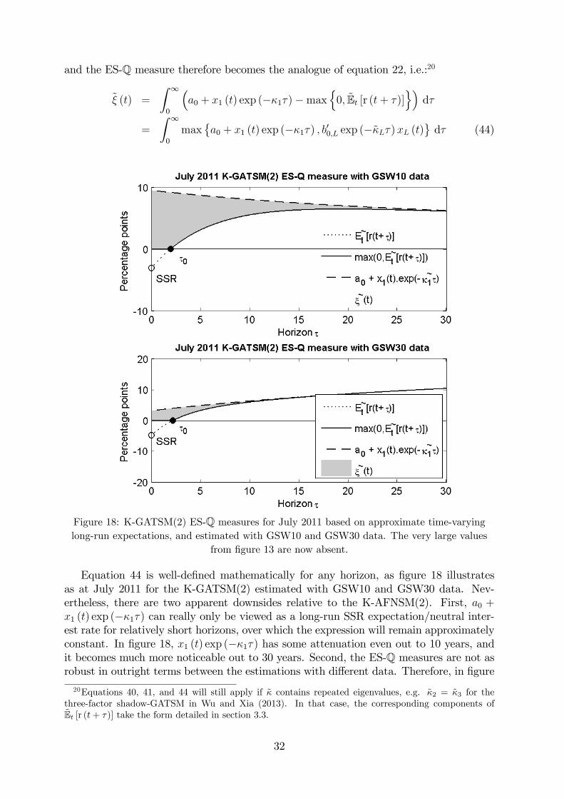
and the ES-Q measure therefore becomes the analogue of equation 22, i.e.:20

ξ (t) =

∫ ∞0

(a0 + x1 (t) exp (−κ1τ)−max

{0, Et [r (t+ τ)]

})dτ

=

∫ ∞0

max{a0 + x1 (t) exp (−κ1τ) , b′0,L exp (−κLτ)xL (t)

}dτ (44)

Figure 18: K-GATSM(2) ES-Q measures for July 2011 based on approximate time-varyinglong-run expectations, and estimated with GSW10 and GSW30 data. The very large values

from figure 13 are now absent.

Equation 44 is well-defined mathematically for any horizon, as figure 18 illustratesas at July 2011 for the K-GATSM(2) estimated with GSW10 and GSW30 data. Nev-ertheless, there are two apparent downsides relative to the K-AFNSM(2). First, a0 +x1 (t) exp (−κ1τ) can really only be viewed as a long-run SSR expectation/neutral inter-est rate for relatively short horizons, over which the expression will remain approximatelyconstant. In figure 18, x1 (t) exp (−κ1τ) has some attenuation even out to 10 years, andit becomes much more noticeable out to 30 years. Second, the ES-Q measures are not asrobust in outright terms between the estimations with different data. Therefore, in figure

20Equations 40, 41, and 44 will still apply if κ contains repeated eigenvalues, e.g. κ2 = κ3 for thethree-factor shadow-GATSM in Wu and Xia (2013). In that case, the corresponding components ofEt [r (t+ τ)] take the form detailed in section 3.3.

32

19, I have again standardized as z scores the time series of ES-Q measures estimated withGSW10 and GSW30 data. The two series, albeit standardized, track each other veryclosely. More importantly, ES-Q measures also line up with the economic recessions, asdiscussed in section 3.4, indicating that they are correlated with output growth and/oroutput gap data.

Figure 19: Time series plots of K-GATMS(2) SSRs and ES-Q measures based on approximatetime-varying long-run expectations, and estimated with GSW10 and GSW30 data. The time

trend evident in figure 14 is now absent.

In summary, stationary K-GATSMs (or B-GATSMs) could be used to obtain ES mea-sures with economic meaning. However, ES measures based on models with an imposedeigenvalue of zero appear to offer a more pragmatic solution; in practice they produce ESmeasures that are robust between different models and data, and the concept of the time-varying long-run SSR expectation/neutral interest rate from the framework also holdsover any horizon.

B ESmeasures from non-block-diagonal specifications

I have used block-diagonal specifications of the mean-reversion matrices in this articleto simplify the notation and resulting expressions. However, ES measures can be calcu-lated analogously with non-block-diagonal specifications. I illustrate this for P measures,

33

because estimation restrictions for GATSMs and shadow-GATSMs are typically appliedunder the Q measure, as mentioned at the end of section 2.2, leaving more flexibility un-der the P measure. However, the results would apply analogously for non-block-diagonalspecifications of mean-reversion matrices under the Q measure.For any K-GATSM (or B-GATSM), the expected path of the state variables under the

physical P measure is:

Et [x (t+ τ)] = θ + exp (−κτ) [x (t)− θ]= θ + exp

(−V DV −1τ

)[x (t)− θ]

= θ + V exp (−Dτ)V −1 [x (t)− θ] (45)

where V DV −1 = κ is a Jordan decomposition (which allows for repeated eigenvalues),with an N × N matrix V containing the eigenvectors in columns and an N × N matrixD containing the blocks of Jordan matrices. Note that the eigensystem decompositioncould potentially result in pairs of complex conjugates (if no additional restrictions areapplied), and that the real parts of the eigenvalues, i.e. real(κi) > 0, need to be positiveto ensure a mean-reverting process. In practice, as with all of the examples in the presentarticle, κ1 inevitably has a single real entry, and so I assume that in what follows. Hence,I denote D as:

D =

[κ1 00 κL

](46)

where κ1 is a scalar, and κL is the (N − 1)× (N − 1) lower block of D. Hence:

exp (−Dτ) =

[exp (−κ1τ) 0

0 exp (−κLτ)

](47)

Equation 45 may be re-expressed with a block diagonal mean-version matrix by pre-multiplying equation 45 by V −1, i.e.:

V −1Et [x (t+ τ)] = V −1θ + exp (−κτ)V −1 [x (t)− θ]Et [x∗ (t+ τ)] = θ∗ + exp (−κτ) [x∗ (t)− θ∗] (48)

where Et [x∗ (t+ τ)] = V −1Et [x (t+ τ)], x∗ (t) = V −1x (t), and θ∗ = V −1θ. Therefore theexpected path of the state variables is equivalently represented by the process:[

Et [x∗1 (t+ τ)]Et [x∗L (t+ τ)]

]=

[θ∗1θ∗L

]+

[exp (−κ1τ) 0

0 exp (−κLτ)

]([x∗1 (t)x∗L (t)

]−[θ∗1θ∗L

])(49)

where the top line contains the expectations process for x∗1 (t), and the bottom line con-tains the expectations process for the remaining elements of x∗ (t), which I denote as the(N − 1)× 1 vector x∗L (t).If κ1 = 0, then exp (−κ1τ) in equation 47 becomes 1, and the GATSM is non-stationary

with a random walk process for x∗1 (t), i.e.:

Et [x∗1 (t+ τ)] = θ∗1 + [x∗1 (t)− θ∗1] = x∗1 (t) (50)

Otherwise, if κ1 & 0, Et [x∗1 (t+ τ)], the GATSM is stationary with a persistent mean-reverting process for x∗1 (t), i.e.:

Et [x∗1 (t+ τ)] = θ∗1 + exp (−κ1τ) [x∗1 (t)− θ∗1] (51)

34

The vector x∗L (t) follows a mean-reverting process, i.e.:

Et [x∗L (t+ τ)] = θ∗L + exp (−κLτ) [x∗L (t)− θ∗L] (52)

Note that these expectations could also be computed directly using matrix exponentials,which is a standard function available in MatLab. However, using a Jordan decompo-sition is faster because it allows for vectorized evaluations of all expectation horizonssimultaneously using scalar exponentials.The expected path of the shadow short rate Et [r (t+ τ)] may be expressed in terms

of Et [x∗ (t+ τ)] as follows:

Et [r (t+ τ)] = a0 + b′0Et [x (t+ τ)]

= a0 + b′0V V−1Et [x (t+ τ)]

= a0 + b∗′0 Et [x∗ (t+ τ)]

= a0 + b∗0,1Et [x∗1 (t+ τ)] + b∗′0,LEt [x∗L (t+ τ)]

= a0 + b∗0,1Et [x∗1 (t+ τ)]

+b∗′0,L {θ∗L + exp (−κLτ) [x∗L (t)− θ∗L]} (53)

where I have left Et [x∗1 (t+ τ)] generic to allow for either non-stationary or stationaryspecifications, and b∗′0 = b′0V . b

∗0 is an N × 1 vector composed of the first element b∗0,1 and

the (N − 1)× 1 lower-block vector b∗0,L. Note that if κ1 > 0 and κ1 = 0, which is the casefor K-AFNSMs with the restriction real(κi) > 0 that is often applied in practice,21 thenthe restriction a0 = 0 applies. The restriction a0 = 0 will also apply if κ1 = 0.With κ1 = 0, the long-run expectation of equation 53 is:

limτ→∞

Et [r (t+ τ)] = b∗0,1 limτ→∞

Et [x∗1 (t+ τ)] + b∗′0,L limτ→∞

Et [x∗L (t+ τ)]

= b∗′0,1x∗1 (t) + b∗′0,Lθ

∗L (54)

and therefore the ES-P measure is:

ξ (t) =

∫ ∞0

(b∗0,1x

∗1 (t) + b∗′0,Lθ

∗L −max {0,Et [r (t+ τ)]}

)dτ

=

∫ ∞0

max{b∗0,1x

∗1 (t) + b∗′0,Lθ

∗L,−b∗′0,L exp (−κLτ) [x∗L (t)− θ∗L]

}dτ (55)

If κ1 & 0, the GATSM is stationary and the approximate long-run expectation of 53is:

limτ→∞

Et [r (t+ τ)] = a0 + b∗0,1Et [x∗1 (t+ τ)] + b∗′0,LEt [x∗L (t+ τ)]

r∞ = a0 + θ∗L + exp (−κLτ) [x∗L (t)− θ∗L] + b∗′0,Lθ∗L (56)

where r∞ is introduced for notational convenience. The ES-P measure is therefore:

ξ (t) =

∫ ∞0

(r∞ −max {0,Et [r (t+ τ)]}) dτ

=

∫ ∞0

max{r∞,−b∗′0,L exp (−κLτ) [x∗L (t)− θ∗L]

}dτ (57)

In summary, ES measures from K-GATSMs specified with non-block-diagonal mean-reversion matrices are analogous to those with block-diagonal specifications, but matrixexponentials or Jordan decompositions are required for the calculation process.21See, e.g Christensen, Diebold, and Rudebusch (2011) footnote 15 or Krippner (2013d).

35

C Alternative ES measures

This appendix provides further discussion on the alternative ES measures mentioned atthe end of section 5.2. I have used the Q measure for the discussions, but the commentswould apply analogously under the P measure.

C.1 Alternative 2

The expression Et [max {0, r (t+ τ)}] does not have a long-run expectation when κ1 = 0,because x1 (t+ τ) has a normal distribution with a mean x1 (t) and a standard deviationthat grows as σ1

√τ . Therefore:

limτ→∞

Et [max {0, r (t+ τ)}] = limτ→∞

Et [max {0, x1 (t+ τ)}] (58)

would be an unbounded positive quantity. The same issue arises for an alternative ESmeasure ξA2 (t) based directly on Et [x1 (t)−max {0, r (t+ τ)}]. For example, using theAFNSM(2) to illustrate, one would obtain the following expression:

ξA2 (t) =

∫ ∞0

Et [x1 (t+ τ)−max {0, x1 (t+ τ)− r (t+ τ)}] (59)

=

∫ ∞0

Et [max {x1 (t+ τ) ,−x2 (t+ τ)}] (60)

ξA2 (t) will be an unbounded positive quantity because x1 (t+ τ) is unbounded onthe positive domain, and that property translates into max {x1 (t+ τ) ,−x2 (t+ τ)}. Atthe same time, max {x1 (t+ τ) ,−x2 (t+ τ)} will be bounded below by −x2 (t+ τ), whichconverges to a finite distribution because x2 (t+ τ) follows a mean-reverting process. Inaddition, x1 (t+ τ) can adopt negative values, which would be questionable from an eco-nomic perspective.If all κi > 0, then an ES measure based on Et [max {0, r (t+ τ)}] would be mathemati-

cally defined. However, the state variable x1 (t+ τ) associated with the eigenvalue κ1 & 0would have the following mean and standard deviation:

mean [x1 (t+ τ)] = exp (−κ1τ) · x1 (t) (61)

stdev [x1 (t+ τ)] = σ1

√1

2κ1[1− exp (−2κ1τ)] (62)

The value of stdev[x1 (t+ τ)] would therefore still be large relative to mean[x1 (t+ τ)]for longer horizons, resulting in the distribution on the positive domain dominating thecalculation of ξA2 (t). In other words, ξA2 (t) would take on large values, sensitive tothe precise magnitude of small estimates of κ1. Therefore, ES-Q measures based onEt [max {0, r (t+ τ)}] with either κ1 = 0 or κ1 & 0 would lack an economic interpretation.

C.2 Alternative 3

A potential alternative to the ES measure proposed in appendix B.1 that would workmathematically in an cases would be to define a measure ξA3 (t) as the analogue of an assetprice by discounting an assumed stream of cashflows with the ZLB term structure. Forexample, assuming a unit cashflow in continuous time would give the following expression:

36

ξA3 (t) =

∫ ∞0

exp [−R¯

(t, u)u] du (63)

where R¯

(t, u) is given in equation 14. Because R¯

(t, u) > 0, ξA3 (t) is a bounded quantityeven if R

¯(t, u) is unbounded (which is the case for B-GATSMs with κ1 = 0; K-GATSMs

interest rates revert to zero for very long horizons). However, such an ES measure wouldneed to justify any particular assumed stream of cashflows, and there would be no conceptof a neutral interest rate underlying it.

37