Measuring the Performance of Schedulability...

Real-Time Systems, 30, 129–154, 2005c© 2005 Springer Science + Business Media, Inc. Manufactured in The Netherlands.

Measuring the Performance of Schedulability Tests∗

ENRICO BINI [email protected] Superiore S. Anna, Pisa, Italy

GIORGIO C. BUTTAZZO [email protected] of Pavia, Pavia, Italy

Abstract. The high computational complexity required for performing an exact schedulability analysis of fixedpriority systems has led the research community to investigate new feasibility tests which are less complex thanexact tests, but still provide a reasonable performance in terms of acceptance ratio. The performance of a test istypically evaluated by generating a huge number of synthetic task sets and then computing the fraction of those thatpass the test with respect to the total number of feasible ones. The resulting ratio, however, depends on the metricsused for evaluating the performance and on the method for generating random task parameters. In particular, animportant factor that affects the overall result of the simulation is the probability density function of the randomvariables used to generate the task set parameters.

In this paper we discuss and compare three different metrics that can be used for evaluating the performance ofschedulability tests. Then, we investigate how the random generation procedure can bias the simulation results ofsome specific scheduling algorithm. Finally, we present an efficient method for generating task sets with uniformdistribution in a given space, and show how some intuitive solutions typically used for task set generation can biasthe simulation results.

Keywords: RM: Rate Monotonic; EDF: Earliest Deadline First; FP: Fixed Priorities; HB: Hyperbolic Bound

1. Introduction

Fixed priority scheduling is the most used approach for implementing real-time applications.When the system consists mostly of periodic activities, tasks are usually scheduled bythe Rate Monotonic (RM) algorithm, which assigns priorities proportionally to the taskactivation rates (Liu and Layland, 1973). Although other scheduling algorithms, like EarliestDeadline First (EDF) (Liu and Layland, 1973) and Least Laxity First (LLF) (Mok, 1983),have been proved to be more effective than RM in exploiting the available computationalresources, RM is still the most used algorithm in industrial systems, mainly for its efficientimplementation, simplicity, and intuitive meaning. In particular, the superior behavior ofEDF over RM has been shown under different circumstances (Buttazzo, 2003), includingoverload conditions, number of preemptions, jitter, and aperiodic service. Nevertheless,the simpler implementation of RM on current commercial operating systems, along with anumber of misconceptions on the two algorithms, seem to be the major causes that preventthe use of dynamic priority schemes in practical applications.

∗This work has been partially supported by the European Union, under contract IST-004527, and by the ItalianMinistry of University Research (MIUR), under contract 2003094275.

130 BINI AND BUTTAZZO

The exact schedulability analysis of fixed priority systems, however, requires high com-putational complexity, even in the simple case in which task relative deadlines are equal toperiods (Joseph and Pandya, 1986; Lehoczky et al., 1995; Audsley et al., 1993). Methodsfor speeding up the analysis of task sets have been recently proposed (Manabe and Aoyagi,1995; Sjodin and Hansson, 1998; Bini and Buttazzo, 2004b), but the complexity of theapproach remains pseudo-polynomial in the worst case. This problem becomes especiallyrelevant for those real-time applications that require an on-line admission control and runon small microprocessors with low processing power.

This fact has led the research community to investigate new feasibility tests that are lesscomplex than exact tests, but still provide a reasonable performance in terms of acceptanceratio. For example, Bini and Buttazzo proposed a sufficient guarantee test, the HyperbolicBound (Bini et al., 2003), that has the same O(n) complexity of the classical utilizationbound proposed by Liu and Layland (1973), but better performance. To increase schedula-bility, Han and Tyan (1997) suggested to modify the task set with smaller, but harmonic,periods using an algorithm of a O(n2 log n) complexity. Other sufficient feasibility testshave been proposed in Burchard et al. (1995) and Lauzac et al. (2003), where additionalinformation on period relations is used to improve schedulability within a polynomial timecomplexity.

A tunable test, called the Hyperplane δ-Exact Test, has recently been proposed (Bini andButtazzo, 2004b) to balance performance versus complexity using a single parameter. Ifδ = 1, the test is exact and hence it has a pseudo-polynomial complexity; if δ < 1 the testbecomes only sufficient and its complexity and performance decrease with δ.

When dealing with approximate tests, the problem of evaluating their performance withrespect to the exact case becomes an important issue. The effectiveness of a guarantee testfor a real-time scheduling algorithm is measured by computing the number of accepted tasksets with respect to the total number of feasible ones. Such a ratio can be referred to as theacceptance ratio. The higher the ratio, the better the test. When the ratio is equal to one,then the guarantee test results to be necessary and sufficient for the schedulability of thetask set.

Computing the acceptance ratio using a rigorous approach is not always possible, exceptfor very simple cases. In all the other cases, the performance of a guarantee test has to beevaluated through extensive simulations, where a huge number of synthetic task sets needto be generated using random parameters. Using this approach, both the evaluation metricsand the way task parameters are generated significantly affect the overall performance ofthe test. This potential biasing factor may lead to wrong design choices if the hypothesesused in the simulation phase differ from the actual working conditions. Unfortunately, toour best knowledge, no much work has been done in the literature to help understandingthese problematic issues.

First, Lehoczky et al. (1989) introduced the breakdown utilization as a means for mea-suring the performance of the Rate Monotonic scheduling algorithm. Then, other au-thors (Park et al., 1995; Chen et al., 2003; Lee et al., 2004) provided methods for com-puting the utilization upper bound, which can indirectly measure the effectiveness of RM.In a previous work, Bini and Buttazzo (2004a) showed the limitations of the former ap-proaches, also proposing a standard metric for evaluating the performance of schedulabilitytests.

MEASURING THE PERFORMANCE OF SCHEDULABILITY TESTS 131

In this paper we introduce a more general framework where the three approaches arediscussed and compared through theoretical results and experimental evidence. The depen-dency between simulation results and task generation routines is discussed, showing howsome intuitive solutions used for generating synthetic task sets can bias the results of thesimulation. A key contribution of this work is an efficient method for generating task setswith uniform distribution in the space of utilizations.

The rest of the paper is organized as follows. Section 2 introduces the metrics commonlyused in the literature for evaluating the performance of feasibility tests, and presents a newevaluation criterion that better describes the properties of a test. Section 3 presents an effi-cient method for generating random task set parameters which does not bias the simulationresults. Section 4 compares the introduced metrics and illustrates some experimental resultscarried out by simulation. Finally, Section 5 states our conclusions.

1.1. Notation and Assumptions

The notation used throughout the paper is reported in Table 1. To make a consistent com-parison among the feasibility tests discussed in this work, the basic assumptions made onthe task set are the same as those typically considered in the real-time literature wherethe original tests have been proposed. That is, each periodic task τi consists of an infinitesequence of jobs τi,k (k = 1, 2, . . . ), where the first job τi,1 is released at time ri,1 = �i

(the task phase) and the generic kth job τi,k is released at time ri,k = �i + (k − 1) Ti . Theworst-case scenario occurs for simultaneous task activations (i.e., �i = 0, i = 1, . . . , n).Relative deadlines are smaller than or equal to periods (Di ≤ Ti ). Tasks are independent(that is, they do not have resource constraints, nor precedence relations) and are fully pre-emptive. Context switch time is neglected. Notice that, although such a simple task modelcan be fruitfully enriched to capture more realistic situations, the objective of this paper innot to derive a new feasibility test, but to clarify some issues related to the performance ofexisting tests, most of which have been derived under the simplifying assumptions reportedabove.

For this reason these simplistic assumptions do not restrict the applicability of the results,but provide a more general framework which allows comparing different results found fordifferent application models.

Table 1. Notation.

Notation Meaning

τi = (Ci , Ti , Di ) The i th periodic taskCi Computation time of task τi

Ti Period of task τi

Di Relative deadline of task τi

Ui = Ci /Ti Utilization of task τi

� = {τ1, . . . , τn} A set of n periodic tasksU = ∑n

1 Ui Utilization of the task setA, B, X = {�1, . . . , �p} A group of task sets (domain)


0 2 4 6 8 10 12

0 2 4 6 8 10 12

τ1

τ1

τ2

τ2RM

EDF

deadline miss

Figure 1. Task set schedulable by EDF, but not by RM.

2. Metrics

It is well known that the RM scheduling algorithm cannot schedule all the feasible task sets.For example, the task set shown in Figure 1 has a total utilization of 1, thus it is schedulableby EDF, but not by RM.

The problem of measuring the difference, in terms of schedulability, between these twoalgorithms has often attracted the interest of the real-time research community. Hence, anumber of methods have been proposed to evaluate the performance of a feasibility test forRM. The most common approaches available in the real-time literature are based on thedefinition of the following concepts:

– Breakdown utilization (Lehoczky et al., 1989);

– Utilization upper bound (Park et al., 1995; Chen et al., 2003; Lee et al., 2004).

Unfortunately, both techniques present some drawback that will be analyzed in detail inSections 2.1 and 2.2. To overcome these problems, a new performance evaluation criterion,the Optimality Degree (OD), will be introduced in Section 2.3.

2.1. Breakdown Utilization

The concept of breakdown utilization was first introduced by Lehoczky et al. (1989) intheir seminal work aimed at providing exact characterization and average case behavior ofthe RM scheduling algorithm.

Definition 1 (Section 3 in Lehoczky et al., 1989). A task set is generated randomly, andthe computation times are scaled to the point at which a deadline is first missed. Thecorresponding task set utilization is the breakdown utilization U ∗

n .

In such a scaling operation, computation times are increased if the randomly generatedtask set is schedulable, whereas they are decreased if the tasks set is not schedulable. Thisscaling stops at the boundary which separates the RM-schedulable and RM-unschedulable


11/2

1/3

1 BA

O

U1

U2

Ci-a

ligne

d

Uub

Uub

U∗

Figure 2. Interpretation of the breakdown utilization.

task sets. Hence, all task sets with the same period configuration that can be obtained byscaling the computation times have the same breakdown utilization, because they all hit theboundary in the same point. We denote these task sets as a group of Ci -aligned task sets.This concept is illustrated in Figure 2.

For example, if we assume the computation times to be uniformly distributed in [0, Ti ](i.e., the Ui uniform in [0, 1]), the number of task sets belonging to the same Ci -alignedgroup is proportional to the length of the O B segment in Figure 2.

Note that a group of Ci -aligned task sets contains more sets when the Ui are similar toeach other, because in this case the segment O B is longer. The utilization disparity in a setof tasks can be expressed through the following parameter, called the U-difference:

δ = maxi {Ui } − mini {Ui }∑n

i=1 Ui. (1)

If δ = 0, all the task utilization factors are the same, whereas δ = 1 denotes the maximumdegree of difference.

We first notice that all the task sets belonging to the same Ci -aligned group have thesame value of δ, since positive scaling factors may be brought outside the min, max and sumoperators in Equation (1), and then simplified. We then show some relationship between aCi -aligned group and its value of U-difference δ.

As it can be argued from Figure 2, when a group of Ci -aligned task sets is characterizedby a small value of δ, the segment O B is longer (that is, the number of task sets in thehypercube (U1, . . . , Un) ∈ [0, 1]n belonging to the same group is larger).

In the case of two tasks, the relationship between δ and |O B| can be explicitly derived.Without any loss of generality, we assume U1 ≤ U2. Since δ does not vary within the sameCi -aligned group, the relation can be computed by fixing any point on the O B segment.


Thus, to simplify the computation, we select the set with U2 = 1. For this group we haveU1 = |AB| (please refer to Figure 2 to visualize the segment AB). Hence:

δ = maxi {Ui } − mini {Ui }∑n

i=1 Ui= U2 − U1

U2 + U1= 1 − |AB|

1 + |AB||AB| = 1 − δ

1 + δ

then:

|O B| =√

1 + |AB|2 =√

2(1 + δ2)

1 + δ. (2)

Note that if δ = 1, then |O B| = 1, whereas if δ = 0, then |O B| = √2.

In the general case of n tasks, the relationship between δ and |O B| cannot be explicitlyfound. However, we can provide an intuition in order to understand it. The longest O Bsegment is equal to the diagonal of a unitary n-dimensional cube, whose length is

√∑n1 12 =√∑n

1 1 = √n, which grows with n. The result illustrated above can be summarized in the

following observation.

Remark 1. When uniformly generating the utilizations (U1, . . . , Un) in [0, 1]n , a groupof Ci -aligned task sets contains more sets if it has a smaller value of U-difference δ. Thisphenomenon becomes more considerable (by a factor

√n) as the number of tasks grows.

These geometrical considerations are very relevant when evaluating the performance ofthe scheduling algorithm. In fact, among all task sets with the same total utilization, RMis more effective on those sets characterized by tasks with very different utilization (i.e.,δ → 1). The intuition behind this statement is also supported by the following facts:

– Liu and Layland proved in 1973 that the worst-case configuration of the utilizationfactors occurs when they are all equal to each other;

– using the Hyperbolic Bound (Bini et al., 2003), which guarantees feasibility if∏n

i=1(1+Ui ) ≤ 2, it has been shown that the schedulability under RM is enhanced when taskshave very different utilizations Ui .

Hence, we can state that:

Remark 2 . For a given total utilization factor U , the feasibility of a task set under the RMscheduling algorithm improves when task utilizations have a large difference, that is whenδ is close to 1.

To further support this remark we have run a simulation experiment in which we gen-erated 106 task sets consisting of n = 8 tasks, whose periods are uniformly distributed in


0 0.1 0.2 0.3 0.4 0.5 0.6 0.7 0.8 0.9 10.7

0.75

0.8

0.85

0.9

0.95

1

U–difference

Bre

akdo

wn

Util

izat

ion

max avg+stdavg avg–stdmin

δ

Figure 3. The breakdown utilization as a function of δ.

[1, 1000]. Computation times are generated so that the set has a specific value of δ. Wethen considered the breakdown utilization U ∗

n (δ) as a random variable. For every value of δ,Figure 3 illustrates the results of the simulation, reporting (from top to bottom) max{U ∗

n (δ)},E[U ∗

n (δ)] + σU ∗n (δ), E[U ∗

n (δ)], E[U ∗n (δ)] − σU ∗

n (δ) and min{U ∗n (δ)}.1 Notice that all values of

min{U ∗n (δ)} are always above the Liu and Layland utilization bound, which, for n = 8, is

0.7241. As predicted by Remark 2, the breakdown utilization increases as δ grows.Summarizing the observations discussed above, we can conclude that when task sets are

randomly generated so that task utilizations have a uniform distribution in the hypercube(U1, . . . , Un) ∈ [0, 1]n , the number of sets with a low value of δ will be dominant. Hence theaverage breakdown utilization will be biased by those task sets with a small U-difference δ,for which RM is more critical. Moreover such a biasing increases as n grows (see Remark 1).Hence, we can state the following remark.

Remark 3. The use of breakdown utilization as a metric for evaluating the performanceof the schedulability algorithms, penalizes RM more than EDF.

The formal proof of the last observation is out of the scope of this paper. However, theintuitive justification we provided so far is confirmed in Section 4 by additional experimentalresults (see Figure 13).

In order to characterize the average case behavior of the RM scheduling algorithm,Lehoczky et al. treated task periods and execution times as random variables, and thenstudied the asymptotic behavior of the breakdown utilization. Their result is expressed bythe following theorem.

Theorem 1 (from Section 4 in Lehoczky et al., 1989). Given task periods uniformlygenerated in the interval [1, B], B ≥ 1, then for n → ∞ the breakdown utilization U ∗

n


converges to the following values:

– if B = 1:

U ∗n = 1 (3)

– if 1 < B ≤ 2:

U ∗n → loge B

B − 1(4)

– if B ≥ 2:

U ∗n → loge B

B�B + ∑�B−1

i=21i

(5)

and the rate of convergence is O(√

n).

Then, the authors derive a probabilistic schedulability bound for characterizing the aver-age case behavior of RM.

Remark 4 (Example 2 in Lehoczky et al., 1989). For randomly generated task sets con-sisting of a large number of tasks (i.e. n → ∞) whose periods are drawn in a uniformdistribution (i.e. hyp. of Th. 1 hold) with largest period ratio ranging from 50 to 100 (i.e.50 ≤ B ≤ 100), 88% is a good approximation to threshold of the schedulability (i.e. thebreakdown utilization) for the rate monotonic algorithm.

The major problem in using this results is that it is based on specific hypotheses aboutperiods and computation times distributions. Such hypotheses are needed to cut some de-grees of freedom on task set parameters and provide a “single-value” result, but they maynot hold for a specific real-time application.

In the next sections, we will overcome this limitation by making the metrics dependenton a specific task set domain.

2.2. Utilization Upper Bound

The utilization upper bound Uub is a well known parameter, used by many authors (Liuand Layland, 1973; Park et al., 1995; Chen et al., 2003; Lee et al., 2004) to provide aschedulability test for the RM algorithm. Following the approach proposed by Chen et al.(2003), the utilization upper bound is defined as a function of a given domain D of task sets.

Definition 2. The utilization upper bound Uub(D) is the maximum utilization such that if atask set is in the domain D and satisfies

∑Ui ≤ Uub then the task set is schedulable. More

formally:

Uub(D) = max

{

Ub :

(

� ∈ D ∧∑

τi ∈�

Ui ≤ Ub

)

⇒ � is schedulable

}

. (6)


From the definition above it follows that:

D1 ⊆ D2 ⇒ Uub(D1) ≥ Uub(D2). (7)

Using this definition, the previous Liu and Layland utilization bound can be expressedas a particular case of Uub. Let Tn be the domain of all sets of n tasks. Then we can writethat:

Uub(Tn) = n( n√

2 − 1) (8)

which is also referred to as utilization least upper bound, because Tn is the largest possibledomain, and hence Uub(Tn) = Ulub is the lowest possible utilization upper bound (seeEq. (7)).

The typical choice for the domain of the task sets is given by fixing task periods anddeadlines. So the domain Mn(T1, . . . , Tn, D1, . . . , Dn), also simply denoted by Mn , is thedomain consisting of all task sets having periods T1, . . . , Tn and deadlines D1, . . . , Dn (soonly the computation times C1, . . . , Cn are varying).

For such a domain, the following result has been found (Chen et al., 2003) when Di = Ti

and TnT1

≤ 2:

Uub

(

Mn ∩ Tn

T1≤ 2 ∩ Di = Ti

)

= 2n−1∏

i=1

1

ri+

n−1∑

i=1

ri − n (9)

where ri = Ti+1

Tifor i = 1, . . . , n − 1.

When n = 2 and r = T2T1

, it was proved (Chen et al., 2003) that:

Uub(M2 ∩ Di = Ti ) = 1 − (r − �r)(�r� − r )

r. (10)

When no restrictions apply on periods and deadlines, the utilization upper bound Uub(Mn),shortly denoted by Uub from now and on, can be found by solving n linear programmingproblems (Park et al., 1995; Lee et al., 2004). The i th optimization problem (for i from 1to n) comes from the schedulability constraint of the task τi . It is formulated as follows:

min(C1,... ,Ci )

i∑

j=1

C j

Tj

subject to

Ci +i−1∑

j=1

⌈ t

Tj

⌉C j ≤ t ∀t ∈ Pi−1(Di )

C j ≥ 0 ∀ j = 1, . . . , i

(11)

where the reduced set of schedulability points Pi−1(Di ), found in Manabe and Aoyagi(1995) and Bini and Buttazzo (2004b), is used instead of the largest one firstly introducedin Lehoczky et al. (1989). If we label the solution of the i th problem (11) as U (i)

ub , the


utilization upper bound is given by:

Uub = mini=1,... ,n

U (i)ub (12)

Once the utilization upper bound Uub is found, the guarantee test for RM can simply beperformed as follows:

n∑

i=1

Ui ≤ Uub. (13)

The utilization bound defined above is tight, meaning that for every value U > Uub thereexists a task set, having utilization U , which is not schedulable by RM. However, a commonmisconception is to believe that the test provided by Eq. (13) is a necessary and sufficientcondition for the RM schedulability, meaning that “all the task sets having total utilizationU > Uub are not schedulable”. Unfortunately, this is not true and the RM schedulability isfar more complex.

In fact, the following lemma holds:

Lemma 1. Given a utilization upper bound Uub < 1, there always exists a task set havingtotal utilization U > Uub which is schedulable by RM.

For the sake of simplicity, the proof will be shown for Di = Ti , but the lemma holdswhen 0 < Di < Ti as well.

Proof: Trivially, every task set having Un = 1 and U1 = · · · = Un−1 = 0 proves thelemma, because it is indeed RM-schedulable and its utilization is 1. However, one mightobject that, since n − 1 utilizations are equal to 0, this set is equivalent to a task set ofa single task, for which Uub = 1, so invalidating the hypothesis for applying the lemma.Seeking an example with a non-trivial task set requires a little extra effort. Lehoczky et al.(1989) showed that a task set is schedulable if:

∀i = 1, . . . , n Ui +i−1∑

j=1

⌈Ti

Tj

⌉Tj

TiU j ≤ 1. (14)

Let us consider a task set having U1 = U2 = · · · = Un−1 = ε and consequently Un =U − (n − 1)ε. By imposing the sufficient condition (14) for the first n − 1 tasks we obtain:

∀i = 1, . . . , n − 1 ε +i−1∑

j=1

⌈Ti

Tj

⌉Tj

Tiε ≤ 1

∀i = 1, . . . , n − 1 ε ≤ 1

1 + ∑i−1j=1

⌈ TiTj

⌉ Tj

Ti


and then:

ε ≤ mini=1,... ,n−1

1

1 + ∑i−1j=1

⌈ TiTj

⌉ Tj

Ti

. (15)

So every choice of ε satisfying Eq. (15) is capable of scheduling the first n − 1 tasks. Toschedule the τn as well, we need that:

U − (n − 1)ε +n∑

j=1

⌈Ti

Tj

⌉Tj

Tiε ≤ 1

then:

ε ≤ 1 − U∑n

j=1

⌈ TiTj

⌉ Tj

Ti− (n − 1)

. (16)

So, to have both Eqs. (15) and (16) true, we select ε such that:

0 < ε ≤ min

{

mini=1,... ,n−1

1

1 + ∑i−1j=1

⌈ TiTj

⌉ Tj

Ti

,1 − U

∑n−1j=1

⌈ TiTj

⌉ Tj

Ti− (n − 1)

}

. (17)

This choice is always possible because the right side of Eq. (17) is strictly positive, due tothe fact that U < 1. Hence the lemma follows.

The previous lemma showes that the condition (13) is not necessary.Nevertheless, Uub is very helpful to understand the goodness of a given period configu-

ration, because it tends to the EDF utilization bound (which is 1) as RM tends to scheduleall the feasible task sets.

In the next section we introduce a new metric that keeps the good properties of theutilization upper bound Uub, still able to provide a measure of all the schedulable task sets.

2.3. OD: Optimality Degree

As stated before, the reason for proposing a new metric is to provide a measure of the realnumber of task sets which are schedulable by a given scheduling algorithm. As for thedefinition of the utilization upper bound, the concept of Optimality Degree (OD) is definedas a function of a given domain D. This a very important property because, if some task setspecification is known from the design phase (e.g., some periods are fixed, or constrainedin an interval), it is possible to evaluate the performance of the test on that specific class oftask sets, by expressing the known information by means of the domain D.


Definition 3. The Optimality Degree ODA (D) of an algorithm A on the domain of tasksets D is:

ODA (D) = |schedA(D)||schedOpt(D)| (18)

where

schedA(D) = {� ∈ D : � is schedulable by A}, (19)

and Opt is any optimal scheduling algorithm.

From this definition it follows that:

– 0 ≤ ODA (D) ≤ 1, for any scheduling algorithm A and for any domain D;

– for any optimal algorithm Opt, ODOpt (D) = 1 for all domains D.

Definition 3 is very general and can be applied to every scheduling algorithm. In thissection we will focus on ODRM (D) and we will consider EDF as a reference for optimality,since our goal is to measure the difference between RM and EDF in terms of schedulabletask sets. In fact, by using the definition of Tn , as the domain of all possible sets of ntasks (see Section 2.2), we can measure the goodness of the RM algorithm by evaluatingODRM (Tn).

However, the domain Tn is hard to be characterized, since the concept of “all the possibletask sets” is too fuzzy. As a consequence, ODRM (Tn) can only be computed by simulation,assuming the task set parameters as random variables with some probability density function(p.d.f.). In order to make the ODRM (Tn) metric less fuzzy and to find some meaningfulresult, we need to reduce the degrees of freedom of domain Tn .

An important classification of the task sets is based on its utilization U . Hence, we couldbe interested in knowing how many task sets are schedulable among those belonging to adomain D with a given utilization U .

Notice that by using the utilization upper bound we can only say that a task set isschedulable if U ≤ Uub(D), but there is still uncertainty among those with U > Uub(D).Instead by using the Optimality Degree the number of schedulable task sets can be measuredby:

ODRM (D, U ) = ODRM

(

D ∩n∑

i=1

Ui = U

)

(20)

The relation between ODRM (D, U ) and Uub(D) is expressed more formally in the fol-lowing Theorem.


Theorem 2. Given a domain of task sets D, the following relationships hold:

ODRM (D, U ) = 1 ∀U ∈ [0, Uub(D)] (21)

0 < ODRM (D, U ) < 1 ∀U ∈ (Uub(D), 1) (22)

Proof: From Definition 2 it follows that all the task sets having utilization U ≤ Uub(D)are schedulable by RM, thus Eq. (21) holds.

From Definition 2, since Uub(D) is the maximum utilization bound there must be sometask set in D which is not schedulable, hence:

ODRM (D, U ) < 1.

From Lemma 1 it follows that for every value of utilization U < 1 it is always possibleto build a task set which is schedulable by RM. Hence:

ODRM (D, U ) > 0

which proves the theorem.

It is worth observing that ODRM (D, U ) does not suffer the weakness of Uub(D), becauseit is capable of measuring the number of schedulable task sets even when the total utilizationexceeds Uub(D).

To derive a numeric value from ODRM (D, U ), we need to model the utilization as arandom variable with a p.d.f. fU (u) and then compute the expectation of ODRM (D, U ).

Definition 4. We define the Numerical Optimality Degree (abbreviated by NOD) as theexpectation of ODRM (D, U ), which is:

NODRM (D) = E[ODRM (D, U )] =∫ 1

0ODRM (D, u) fU (u)du. (23)

As for the average 88% bound derived by Lehoczky et al., in order to achieve a numericalresult we have to pay the price of modelling a system quantity (the utilization U ) by arandom variable. If we assume the utilization uniform in [0, 1] Eq. (23) becomes:

NODRM (D) =∫ 1

0ODRM (D, u) du (24)

which finalizes our search. In fact, this value well represents the fraction of the feasible tasksets which are schedulable by RM in the following hypotheses:

– the task sets belong to D;

– the utilization of the task sets is a uniform random variable in [0, 1].


Moreover, as expected, we have that:

∫ 1

0ODRM (D, u) du =

∫ Uub(D)

0ODRM (D, u) du +

∫ 1

Uub(D)ODRM (D, u) du =

∫ Uub(D)

01 du +

∫ 1

Uub(D)ODRM (D, u) du = Uub(D) +

∫ 1

Uub(D)ODRM (D, u) du

and then:

∫ 1

0ODRM (D, u) du ≥ Uub(D) (25)

which shows that NOD is less pessimistic than Uub.

3. Synthetic Task Set Generation

The typical way to measure the performance of a guarantee test is to randomly generatea huge number of synthetic task sets and then verify which percentage of feasible setspass the test. However, the way task parameters are generated may significantly affect theresult and bias the judgement about the schedulability tests. In this section we analyze somecommon techniques often used to randomly generate task set parameters and we highlighttheir positive and negative aspects.

3.1. Generating Periods

Under fixed priority scheduling, task periods significantly affect the schedulability of a taskset. For example, it is well known that, when

∀i = 1, . . . , n − 1 Ti evenly divides Ti+1

and relative deadlines are equal to periods, then any task set with total utilization less thanor equal to 1 can be feasibly scheduled by RM (Kuo and Mok, 1991), independently of thecomputation times.

Whereas task execution times can have great variations, due to the effect of several low-level architecture mechanisms or to the complex structure of a task, task periods are moredeterministic, since are defined by the user and then enforced by the operating system. Asa consequence, the assumption of treating task periods as random variables with uniformdistribution in a given interval may not reflect the characteristics of real applications andcould be inappropriate for evaluating a schedulability test. For example, using a uniformp.d.f., possible harmonic relations existing among the periods cannot be replicated.

On the other hand, at an early stage of evaluating a guarantee test without any a prioriknowledge about the environment where it is going to be used, assuming some probabilitydensity for the period is something we cannot avoid.


3.2. Computation Times Generation

Once task periods have been selected, running a guarantee test in the whole space of taskset configurations requires computation times to be generated with a given distribution. Inthe absence of specific knowledge of application task, a common approach is to assumethe computation time Ci uniform in [0, Ti ]. Notice that, since computation times Ci andutilizations Ui differ by a scaling factor of Ti , this is equivalent of assuming each Ui to beuniform in [0, 1].

Considering the dependency of some schedulability test from the total processor utiliza-tion, a desirable feature of the generation algorithm is the ability to create synthetic task setswith a given utilization factor U . Hence, individual task utilizations Ui should be generatedwith a uniform distribution in [0, U ], subject to the constraint

∑Ui = U . Implementing

such an algorithm, however, hides some pitfalls. In the next paragraphs we will describesome “common sense” algorithms, discuss their problems, and then propose a new efficientmethod.

3.3. The UScaling Algorithm

A first intuitive approach, referred to as the UScaling algorithm, is to generate the Ui ’s in[0, U ] and then scale them by a factor U∑n

1 Ui, so that the total processor utilization is exactly

U . The UScaling algorithm has an O(n) complexity and, using Matlab syntax,2 can becoded as shown in Figure 4.

Unfortunately, the algorithm illustrated above incurs in the same problem discussed inSection 2.1 for the scaling of Ci -aligned task sets, whose effect was to bias the breakdownutilization. Here, the consequence of the scaling operation is that task sets having similarUi ’s (those with δ close to 0) are generated with higher probability.

Figure 5 illustrates the values of 5000 utilization tuples, generated by the UScaling al-gorithm with n = 3 and U = 1. As expected, the generated values are more dense aroundthe point where all the Ui are equal to U/n. As argued in Remark 2, these task sets arepenalized by RM, hence generating the utilizations by the UScaling algorithm is pessimisticfor RM.

3.4. The UFitting Algorithm

A second algorithm for generating task sets with a given utilization U consists in makingU1 uniform in [0, U ], U2 uniform in [0, U − U1], U3 uniform in [0, U − U1 − U2], and so

function vectU = UScaling(n, U)vectU = rand(1,n);vectU = vectU.∗U ./sum(vectU);

Figure 4. Matlab code for the UScaling algorithm.


0

0.2

0.4

0.6

0.8

1

0

0.2

0.4

0.6

0.8

1

0

0.2

0.4

0.6

0.8

1

U1U2

U3

Figure 5. Result of the UScaling algorithm.

function vectU = UFitting(n, U)upLimit = U ;for i=1:n−1,

vectU(i) = rand∗upLimit;upLimit = upLimit−vectU(i);

endvectU(n) = upLimit;

Figure 6. Matlab code for the UFitting algorithm.

on, until Un is deterministically set to the value Un = U − ∑n−1i=1 Ui . This method, referred

to as UFitting, is described by the code illustrated in Figure 6.The UFitting algorithm has an O(n) complexity, but it has the major disadvantage of being

asymmetrical, meaning that the U1 has a different distribution than U2, and so forth.Moreover, as depicted in Figure 7, the achieved distribution is again not uniform, and

task sets having different values of Ui ’s (those with δ close to 1) are generated with higherprobability. Hence, for the same reasons stated in Remark 2, generating the utilizations bythe UFitting algorithm favors RM with respect to EDF.

3.5. The UUniform Algorithm

The problems previously encountered can be solved through the method depicted in Figure 8,referred to as the UUniform algorithm.


0

0.2

0.4

0.6

0.8

1

0

0.2

0.4

0.6

0.8

1

0

0.2

0.4

0.6

0.8

1

U1U2

U3

Figure 7. Result of the UFitting algorithm.

function vectU = UUniform(n, U)while 1

vectU = U .∗rand(1,n−1);if sum(vectU) <= U % boundary condition

breakend

endvectU(n) = U−sum(vectU);

Figure 8. Matlab code for the UUniform algorithm.

As depicted in Figure 9, the UUniform algorithm generates task utilizations with uniformdistribution.

The problem with this algorithm, however, is that it has to run until the boundary conditionis verified once (see the code of UUniform). As proved by Bini et al. (2003) the probabilityof such an event is 1/(n − 1)!, hence the average number of iterations needed to generatea single tuple is (n − 1)!, which makes the algorithm unpractical.

3.6. The UUniFast Algorithm

To efficiently generate task sets with uniform distribution and with O(n) complexity, weintroduce a new algorithm, referred to as the UUniFast algorithm. It is built on the consider-ation that the p.d.f. of the sum of independent random variables is given by the convolution


0

0.2

0.4

0.6

0.8

1

0

0.2

0.4

0.6

0.8

1

0

0.2

0.4

0.6

0.8

1

U1U2

U3

Figure 9. Result of the UUniform algorithm.

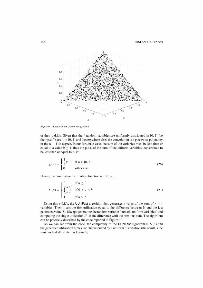
of their p.d.f.’s. Given that the i random variables are uniformly distributed in [0, 1] (sotheir p.d.f.’s are 1 in [0, 1] and 0 everywhere else) the convolution is a piecewise polynomyof the (i − 1)th degree. In our fortunate case, the sum of the variables must be less than orequal to a value b ≤ 1, thus the p.d.f. of the sum of the uniform variables, constrained tobe less than or equal to b, is:

fi (u) =

1

bui−1 if u ∈ [0, b]

0 otherwise(26)

Hence, the cumulative distribution function (c.d.f.) is:

Fi (u) =

0 if u ≤ 0(

u

b

)i

if 0 < u ≤ b

1 if u > b

(27)

Using this c.d.f.’s, the UUniFast algorithm first generates a value of the sum of n − 1variables. Then it sets the first utilization equal to the difference between U and the justgenerated value. So it keeps generating the random variable “sum of i uniform variables” andcomputing the single utilization Ui as the difference with the previous sum. The algorithmcan be precisely described by the code reported in Figure 10.

As we can see from the code, the complexity of the UUniFast algorithm is O(n) andthe generated utilization tuples are characterized by a uniform distribution (the result is thesame as that illustrated in Figure 9).


function vectU = UUniFast(n, U)sumU = U ;

for i=1:n−1,nextSumU = sumU.∗randˆ(1/(n−i));vectU(i) = sumU − nextSumU;sumU = nextSumU;

endvectU(n) = USum;

Figure 10. Matlab code for the UUniFast algorithm.

function vectU = UUniSort(n, U)v = [0, rand(1,n−1), U ];sumU = sort(v);vectU = sumU(2:n+1)−sumU(1:n);

Figure 11. Matlab code for the UUniSort algorithm.

3.7. The UUniSort Algorithm

A more elegant version of the algorithm for achieving a uniform distribution is to generaten −1 uniform values in [0, U ], add 0 and U to the vector, sort it, and then set the utilizationsequal to the difference of two adjacent values (Marzario, 2004). This algorithm, referred toas UUniSort, is coded as shown in Figure 11.

Note that the UUniSort algorithm, although more elegant than UUniFast, has anO(n log(n)) complexity.

3.8. Comparing The Algorithms

Figures 5 and 7 qualitatively show the uneven distribution of the generated task sets inthe utilization space for the UScaling and the UFitting algorithm, respectively. A quantita-tive measure of the resulting distribution can be provided by computing the U-differenceparameter defined in Eq. (1).

Figure 12 shows the probability density function of the U-difference, when n = 8 and2 · 105 random task sets are generated.

As expected, the utilizations generated by the UScaling algorithm are characterized byvalues of U-difference close to zero, meaning that the utilization values tend to be similarto each other. On the other hand, the utilizations generated by the UFitting algorithm differmuch more, as proved by the long tail of the related U-difference density function.

4. Metrics Comparison

In this section we present a set of simulation experiments aimed at comparing the threemetrics discussed in the paper. Although the numerical results provided here are not intended


0 0.05 0.1 0.15 0.2 0.25 0.3 0.35 0.4 0.45 0.5 0.55 0.6 0.65 0.7 0.75 0.8 0.85 0.9 0.95 10

2

4

6

8

10

delta

prob

abili

ty d

ensi

ty fu

nctio

ns p.d.f. of delta using UScaling methodp.d.f. of delta using UUniFast methodp.d.f. of delta using UFitting method

Figure 12. Value of δ for different generation methods.

to be an absolute measure of the RM schedulability, the objective of this work is to showthat RM is capable of scheduling many more task sets than commonly believed.

Comparing the three metrics is not trivial, because they have different definitions andrequire different simulations. More specifically, while the utilization upper bound Uub de-pends only on periods and deadlines, both the breakdown utilization U ∗ and the optimalitydegree OD also depend on the computation times (i.e., on the utilizations). Hence, the algo-rithm selected for the random generation of the computation times/utilizations may affectthe results.

Two groups of experiments are presented: the first group is intended to check the influenceof the random parameters generation routines on the considered metrics; the second groupis aimed at testing how period relations affect the metrics.

4.1. Effects of the Generation Algorithm

The first two experiments show the influence of the generation algorithm on the metrics.We remind that Uub does not depend on the computation times of the tasks set. For thisreason, this subsection only compares the breakdown utilization U ∗

n with the OptimalityDegree ODRM (D, U ). The simulation was carried out by fixing the periods and deadlines,and then generating the computation times. Note that this choice is not restrictive, becausethe distribution of U ∗

n and ODRM (D, U ) scales with Uub. Task periods were set to the valuesshown in Table 2.

In Table 2 all the U (i)ub are reported. The computation times where the optimal solution of

the problem in Eq. (11) occurs is reported as well. As you can notice, the schedulability ofthe task τi is not influenced in any way by all the lower priority tasks. This fact is representedin the table by the symbol “-”. For the specific period selection, Uub is given by the minimumamong the numbers in the fourth column, which is 9

10 = 0.9.Considering the Definition 1, we expect the breakdown utilization to be always greater

than the Uub. This fact is confirmed by the simulation results reported in Figure 13. In thisexperiment, 2 · 105 tuples have been generated for each method described in Section 3. The


Table 2. Task set parameters.

where U (i)ub occurs

i Ti Di U (i)ub C1 C2 C3 C4 C5 C6

1 3 3 1 3 − − − − −2 8 8 11

12 = 0.9167 2 2 − − − −3 20 20 9

10 = 0.9 0 4 8 − − −4 42 42 201

210 = 0.9571 1 0 2 22 − −5 120 120 201

210 = 0.9571 0 0 0 36 12 −6 300 300 9

10 = 0.9 0 0 0 0 60 120

0.89 0.9 0.91 0.92 0.93 0.94 0.95 0.96 0.97 0.98 0.99 10

0.2

0.4

0.6

0.8

1

utilization

cum

ulat

ive

dist

ribut

ion

func

tions

c.d.f. BU (used UScaling method)c.d.f. BU (used UUniFast method)c.d.f. BU (used UFitting method)Uub = Uub(3) = Uub(6) = 0.9000 Uub(2) = 0.9167 Uub(4) = Uub(5) = 0.9571

Figure 13. c.d.f. of U∗ for different algorithms.

plots in the figure clearly show the biasing factor introduced by the different generationalgorithms. In fact, the breakdown utilization has a larger c.d.f. when tasks are generatedwith the UScaling algorithm, meaning that RM is penalized. The opposite effect occurs whentasks are generated with UFitting, which favors RM more than under the uniform distributionproduced by UUniFast. As synthetic values for the c.d.f.’s we can use the expectation of thethree breakdown utilization random variables obtained by the three different methods, thatis

E[U ∗|UScaling] = 0.9296,

E[U ∗|UUniFast] = 0.9372,

E[U ∗|UFitting] = 0.9545.

However, as extensively discussed in Section 2.1, the breakdown utilization is not a fairmetric for evaluating the difference between RM and EDF in terms of schedulability. Forthis purpose, the Optimality Degree (OD) has been introduced in Section 2.3. Figure 14reports the OD values as a function of the total utilization and for different generationmethods.


0.89 0.9 0.91 0.92 0.93 0.94 0.95 0.96 0.97 0.98 0.99 10

0.2

0.4

0.6

0.8

1

utilization

OD

(U) OD(U) (used UScaling method)

OD(U) (used UUniFast method) OD(U) (used UFitting method) Uub = Uub(3) = Uub(6) = 0.9000Uub(2) = 0.9167 Uub(4) = Uub(5) = 0.9571

Figure 14. OD for different algorithms.

In this experiment, 3·105 task sets are generated, 5000 for each value of the utilization.The insight we derive is consistent with the previous experiment: the UScaling algorithmpenalizes RM more than UUniFast, whereas UFitting favors RM by generating easier tasksets.

Assuming the total utilization is uniform in [0, 1], the NOD parameter (see Definition 4and Eq. (24)) is computed for the three methods:

NOD|UScaling = 0.9679

NOD|UUniFast = 0.9739

NOD|UFitting = 0.9837

showing a much better behavior of RM than expected with the breakdown utilization. Theresult of the experiments are summarized in Table 3.

The metric we consider more reliable is NOD|UUniFast, because it is related to the realpercentage of feasible task sets and it refers to task sets uniformly distributed in the utilizationspace. As a consequence, in the next simulations, the UUniFast algorithm is adopted forgenerating the utilizations Ui .

Table 3. Schedulability results for RM.

Metric Value

Uub(Mn) 0.9E[ U∗|UScaling] 0.9296E[ U∗|UUniFast] 0.9372E[ U∗|UFitting] 0.9545NOD|UScaling 0.9679NOD|UUniFast 0.9739NOD|UFitting 0.9837


2 3 4 5 6 7 8 9 100.75

0.8

0.85

0.9

0.95

1

n = number of tasks

met

rics

UubBU NOD

Figure 15. Metrics as a function of n.

4.2. Effects of the Task Set Parameters

In the two experiments described in this section task periods are uniformly generated in[1, B] and then utilizations are generated by the algorithm UUniFast. The objective ofthe experiments is to compare the metrics E[Uub], E[U ∗] and E[NOD]. For the sake ofsimplicity, we will omit the expectation operator E[·].

The objective of the first experiment is to study the dependency of the metrics on thenumber n of tasks. To do that, we set B = 100 and generated a total number of 2 · 104 tasksets. As expected, all the metrics report a decrease in the schedulability under RM and theyare ordered in a way similar to the first experiment.

The second experiment of this section aims at considering the dependency of the metricson the task periods. To do so, we set n = 4 and let B vary in the interval [1, 104]. We

100

101

102

103

104

0.8

0.82

0.84

0.86

0.88

0.9

0.92

0.94

0.96

0.98

1

B = periods upper bound

met

rics

UubBU NOD

Figure 16. Metrics as a function of periods.


generated 5 · 104 task sets. The result is reported in Figure 16. When B = 1 the periods areall the same value. The value of 1 is then what we expected.

In addition, all the three metrics seems to have a minimum for B = 2. This fact is alsoconfirmed by the asymptotical study of the breakdown utilization (reported in Theorem 1)and by many different proofs in the real-time literature (Liu and Layland, 1973; Burchardet al., 1995; Chen et al., 2003; Bini et al., 2003) which show this phenomenon.

5. Conclusions

The motivation for writing this paper has been to analyze in great detail how the methodologyused for evaluating the performance of fixed priority scheduling algorithms affects theresults. In particular, we have considered two metrics commonly used in the literature andshowed that both the breakdown utilization and the utilization upper bound can be unfairin judging the performance of the Rate/Deadline Monotonic scheduling algorithms. Wealso illustrated that significant biasing factors can be introduced by the routines used forgenerating random task sets.

The main result achieved from this study is that current metrics intrinsically evaluatethe behavior of RM in pessimistic scenarios, which are more critical for fixed priorityassignments than for dynamic systems. The use of unbiased metrics, such as the OptimalityDegree, shows that the penalty payed in terms of schedulability by adopting fixed priorityscheduling is less than commonly believed.

Notes

1. E[X ] denotes the expectation of the random variable X , and σX denotes its standard deviation.2. We remind that in Matlab arrays can be assigned using the same syntax used for variables.

References

Audsley, N. C., Burns, A., Richardson, M., Tindell, K. W., and Wellings: A. J. 1993. Applying new schedulingtheory to static priority pre-emptive scheduling.Software Engineering Journal 8(5): 284–292.

Bini, E., and Buttazzo, G. C. 2004a. Biasing effects in schedulability measures. In: Proceedings of the 16thEuromicro Conference on Real-Time Systems. Catania, Italy, pp. 196–203.

Bini, E., and Buttazzo, G. C. 2004b. Schedulability analysis of periodic fixed priority systems. IEEE Transactionson Computers 53(11): 1462–1473.

Bini, E., Buttazzo, G. C., and Buttazzo, G. M. 2003. Rate monotonic scheduling: The hyperbolic bound. IEEETransactions on Computers 52(7): 933–942.

Burchard, A., Liebeherr, J., Oh, Y., and Son, S. H. 1995. New strategies for assigning real-time tasks to multipro-cessor systems. IEEE Transactions on Computers 44(12): 1429–1442.

Buttazzo, G. C. 2003. Rate monotonic vs. EDF: Judgment day. In: Proceedings of the EMSOFT. Philadelphia, PAUSA, pp. 67–83.

Chen, D., Mok, A. K., and Kuo, T.-W. 2003. Utilization bound revisited. IEEE Transaction on Computers 52(3):351–361.

Han, C.-C., and Tyan, H.-y. 1997. A better polynomial-time schedulability test for real-time fixed-priority schedul-ing algorithm. In: Proceedings of the 18th IEEE Real-Time Systems Symposium. San Francisco, CA USA.

Joseph, M., and Pandya, P. K. 1986. Finding response times in a real-time system. The Computer Journal 29(5):390–395.


Kuo, T.-W., and Mok, A. K. 1991. Load adjustment in adaptive real-time systems’. In: Proceedings of the 12thIEEE Real-Time Systems Symposium. San Antonio, TX USA, pp. 160–170.

Lauzac, S., Melhem, R., and Mosse, D. 2003. An improved rate-monotonic admission control and its applcations.IEEE Transactions on Computers 52(3): 337–350.

Lee, C.-G., Sha, L., and Peddi, A. 2004. Enhanced utilization bounds for QoS management. IEEE Transactionson Computers 53(2): 187–200.

Lehoczky, J. P., Sha, L., and Ding, Y. 1989. The rate-monotonic scheduling algorithm: Exact characterization andaverage case behavior. In: Proceedings of the 10th IEEE Real-Time Systems Symposium. Santa Monica, CAUSA, pp. 166–171.

Lehoczky, J. P., Sha, L., and Strosnider, J. K. 1995. The deferrable server algorithm for enhanced aperiodicresponsiveness in hard real-time environment. IEEE Transactions on Computers 44(1): 73–91.

Liu, C. L., and Layland, J. W. 1973. Scheduling algorithms for multiprogramming in a hard real-time environment.Journal of the ACM 20(1): 46–61.

Manabe, Y., and Aoyagi, S. 1995. A feasibility decision algorithm for rate monotonic scheduling of periodicreal-time tasks. In: Proeedings. of the 1st Real-Time Technology and Applications Symposium. pp. 297–303.

Marzario, L. 2004. Personal communication.Mok, A. K. 1983. Fundamental design problems of distributed systems for the hard-real-time environment. Ph.D.

thesis, Dept. of Electrical Engineering and Computer Science, Massachusetts Institute of Technology, Boston,MA USA.

Park, D.-W., Natarajan, S., Kanevsky, A., and Kim, M. J. 1995. A generalized utilization bound test for fixed-priority real-time scheduling’. In: Proceedings of the 2nd International Workshop on Real-Time Systems andApplications. Tokyo, Japan, pp. 73–77.

Sjodin, M., and Hansson, H. 1998. Improved response-time analysis calculations. In: Proceedings of the 19thIEEE Real-Time Systems Symposium. Madrid, Spain, pp. 399–408.

Enrico Bini received the Ph.D. in Computer Engi-neering from Scuola Superiore Sant’Anna in Pisa, inOctober 2004. In 2000 he received the Laurea degree inComputer Engineering from “Universita di Pisa” and,one year later, he obtained the “Diploma di Licenza”from the Scuola Superiore Sant’Anna. In 1999 he stud-ied at Technische Universiteit Delft, in the Nederlands,by the Erasmus student exchange program. In 2001he worked at Ericsson Lab Italy in Roma. In 2003 hewas a visiting student at University of North Carolinaat Chapel Hill, collaborating with prof. Sanjoy Baruah.His research interests cover scheduling algorithms,real-time operating systems, embedded systems designand linear programming.

Giorgio Buttazzo is an Associate Professor of Com-puter Engineering at the University of Pavia, Italy. Hegraduated in Electronic Engineering at the Universityof Pisa in 1985, received a Master in Computer Scienceat the University of Pennsylvania in 1987, and a Ph.D.in Computer Engineering at the Scuola Superiore S.Anna of Pisa in 1991. During 1987, he worked on ac-tive perception and real-time control at the G.R.A.S.P.

Measuring the Performance of Schedulability...

Documents

Transcript of Measuring the Performance of Schedulability...