NBER WORKING PAPER SERIES

MEASURING THE OUTPUT AND PRICES OF THE LOTTERY SECTOR:AN APPLICATION OF IMPLICIT EXPECTED UTILITY THEORY

Kam Yu

Working Paper 14020http://www.nber.org/papers/w14020

NATIONAL BUREAU OF ECONOMIC RESEARCH1050 Massachusetts Avenue

Cambridge, MA 02138May 2008

The author wishes to thank Lottery Canada for providing the data on Lotto 6/49. The views expressedherein are those of the author(s) and do not necessarily reflect the views of the National Bureau ofEconomic Research.

NBER working papers are circulated for discussion and comment purposes. They have not been peer-reviewed or been subject to the review by the NBER Board of Directors that accompanies officialNBER publications.

© 2008 by Kam Yu. All rights reserved. Short sections of text, not to exceed two paragraphs, maybe quoted without explicit permission provided that full credit, including © notice, is given to the source.

Measuring the Output and Prices of the Lottery Sector: An Application of Implicit ExpectedUtility TheoryKam YuNBER Working Paper No. 14020May 2008JEL No. C43,D81,L83

ABSTRACT

Using implicit expected utility theory, a money metric of utility derived from playing a lottery gameis developed. Output of the lottery sector can be defined as the difference in utility with and withoutthe game. Using a kinked parametric functional form, outputs of the Canadian Lotto 6/49 are estimated.Results show that this direct economic approach yield an average output which is almost three timesof the official GDP, which takes total factor costs as output. A by-product of the estimation is an implicitprice index for lottery, which can serve as a cost-of-living index for the CPI. The estimated price elasticityof demand -0.67 closely resembles results for the U.K. and Israel in previous studies.

Kam YuLakehead Universitykam.yu@lakeheadu.ca

Measuring the Output and Prices of the LotterySector: An Application of Implicit Expected Utility

Theory

Kam Yu∗

November 30, 2006

Abstract

Using implicit expected utility theory, a money metric of utility derivedfrom playing a lottery game is developed. Output of the lottery sector canbe defined as the difference in utility with and without the game. Using akinked parametric functional form, outputs of the Canadian Lotto 6/49 areestimated. Results show that this direct economic approach yield an averageoutput which is almost three times of the official GDP, which takes total factorcosts as output. A by-product of the estimation is an implicit price index forlottery, which can serve as a cost-of-living index for the CPI. The estimatedprice elasticity of demand -0.67 closely resembles results for the U.K. and Is-rael in previous studies.

JEL Classification: C43, D81, H50, L83, O47, P44Keywords: system of national accounts, direct measurement, volume index,quantity index, choice under risk, lotteries, Lotto 6/49, gambling, non-expectedutility theory.

1 Introduction

This paper studies the output and price measurement of the lottery sector using aneconomic approach. Perhaps as a result of the accumulating effects in jackpots whenthere are no major prize winners in previous weeks, lottery industries in Canadaand elsewhere are growing steadily. In 1997, according to the Survey of HouseholdSpending (SHS), 68.4% of all households in Canada bought government-run pool and

∗Lakehead University, e-mail: Kam.Yu@lakeheadu.ca. The author wishes to thank LotteryCanada for providing the data on Lotto 6/49.

1

lottery tickets, with the average expenditure per household equals to $238, whichtranslates to 0.3% of total expenditure. Expenditure in gambling, however, has beenfound to be consistently under-reported in the SHS. The actual amount of moneyspent on gambling, according to revenue reported by the government, is three timesthe amount reported by households (Marshall, 1998, p.31). Therefore the lotteryindustry has become a significant part of the GDP, and a more accurate methodof measuring its output is needed. Moreover, prices in any game of chance are notcurrently included in the consumer price index (CPI). If we are able to calculate thereal output of lottery, then an implicit price index can also be computed. This priceindex can be used both as a deflator in the national account and as a subindex inthe CPI.

In the theory of consumption under uncertainty, the typical consumer is tradi-tionally assumed to follow an optimal statistical decision rule with risk-averse prefer-ences. This leads to the well known expected utility hypothesis (EUH), in which therisk averseness is often assumed to be decreasing in wealth. A wealthy person is morewilling to invest in a risky but high yield portfolio than an average person. The EUHhas been successfully applied to problems in insurance and financial investment. Itslinear structure, however, also implies that a risk-averse expected utility maximizerwill never buy lottery tickets unless the payout prizes are exceedingly large. In re-ality we observe that consumers who are fully insured in their houses and cars alsoengage in a variety of gambling activities. Therefore we need a different approachother than the EUH. In the past two decades new theories on economic uncertaintyhave been developed. For example, Diewert (1995) shows that the real output of asimple gambling sector can be measured using implicit expected utility theory. Itsuccessfully models consumers’ risk-averseness involving large portion of their wealthand at the same time captures the risk-seeking character involving small amount ofmoney. In this paper, Diewert’s model will be generalized from a simple two-outcomelottery to an N -outcome one (the 6/49 lotto has 6 outcomes with different payouts).The functional form of the estimating equation will be derived and estimated withCanadian data.

The portion of government output in the national accounts of industrialized coun-tries has been increasing over the past several decades. There has been an ongoingdebate on the concept and practice of measuring government output. Due to theabsence of market prices in government services, statistical agencies traditionally usetotal factor costs as a proxy for the output. This practice has become less acceptableas the government sector has expanded. The Inter-Secretariat Working Group onNational Accounts (1993)1 recommends that government output should be measureddirectly whenever possible. In fact, the statistical bureaus in Australia, U.K. and theNetherlands have switched to various forms of direct methods recently. In the case ofgovernment lotteries, the price of a lottery ticket is not the market price in the sense

1This manual is often referred to as SNA93.

2

of quantity measurement. Therefore the total factor cost is usually taken as a proxyfor output. This paper proposes a direct method of measuring government servicesin lotteries. Our results show that by using a direct utility approach, the measuredoutput of Lotto 6/49 in Canada is three times higher than the official statistics. Theestimated price elasticity of demand is found to be very similar to those of othercountries.

The structure of the paper is as follows. Section 2 examines the classical andnew economic theories of uncertainty and some of their applications. In section 3,we briefly discuss the gambling sector in Canada and apply the new theory to theeconomics of lottery. A money metric measure of the real output of the sector willbe derived. In practice, a two-parameter equation is estimated using a nonlinearregression. The next step is to use the Canadian Lotto 6/49 as an example to testthe feasibility of the model. The results are presented in section 4. Finally, section 5concludes.

2 The Economic Analysis of Uncertainty: A Brief

Review

2.1 The Expected Utility Hypothesis

The classical analysis of economic uncertainty begins with Friedman and Savage(1948) and von Neumann and Morgenstern (1953). Their writings form the basisfor what is generally known as expected utility hypothesis (EUH). The EUH hasbeen successfully applied to a number of economic problems such as asset pricingand insurance. It has also been used as the premise in statistical decision theory.2

In the basic model, the uncertainty is represented by a set of simple lotteries Lover a set of outcomes C. A simple lottery L ∈ L in the discrete case can berepresented by a vector of outcomes and a vector of probabilities, that is, L =(p1, p2, . . . , pN) where

∑Ni=1 pi = 1. Therefore outcome Ci ∈ C will occur with

probability pi, i = 1, . . . , N . A consumer or a decision maker is assumed to have acomplete and transitive preference structure % on L. In addition, the preferencesare supposed to be continuous and independent. The latter assumption means thatfor all L, L′, L′′ ∈ L, and 0 < α < 1, we have

L % L′ if and only if αL + (1− α)L′′ % αL′ + (1− α)L′′.

Therefore, the ranking on L and L′ remains unchanged if we mix the lotteries withanother one to form compound lotteries. Together, the continuity and independence

2See, example, Luce and Raiffa (1957) and Pratt, Raiffa, and Schaifer (1995).

3

assumptions imply the existence of an expected utility function U : L → R such that

U(L) =N∑

i=1

uipi, (1)

where ui, i = 1, . . . , N are utility numbers assigned to the outcomes Ci ∈ C respec-tively. Therefore,

L % L′ if and only if U(L) ≥ U(L′).

The independence assumption, which gives rise to the linear structure of the expectedutility function, has been controversial from the beginning. Samuelson (1952) defendsthe independence axiom by arguing that in a stochastic situation, the outcomes Ci

are mutually exclusive and therefore are statistically independent. ConsequentlyU(L) must be additive in structure. Moreover, using a theorem by Gorman (1968),Blackorby, Davidson, and Donaldson (1977) show that continuity and independenceimply that the utility structure under uncertainty is additively separable.

In spite of its solid theoretical foundation and normative implications, some ap-plications of the EUH do not conform well with real behaviour.3 The most seriouschallenge is the Allais (1953) paradox, which can be illustrated by the following ex-ample. It involves decisions over two pairs of lotteries. The outcomes are cash prizes(C1, C2, C3) = ($2, 500, 000; $500, 000; 0). In the first pair, the subjects are askedto choose between L1 = (0, 1, 0) and L′

1 = (0.10, 0.89, 0.01). That is, L1 is getting$500,000 for sure, while L′

1 has a 10% chance of winning $2,500,000, 89% chance ofwinning $500,000, and a 1% chance of winning nothing. The second part involvingchoosing between L2 = (0, 0.11, 0.89) and L′

2 = (0.10, 0, 0.90). Allais claims thatmost people choose L1 and L′

2. This contradicts the EUH since if we denote u25, u05,and u0 to be the utility numbers correspond to the three prizes, then L1 � L2 meansthat

u05 > 0.1u25 + 0.89u05 + 0.01u0.

Adding 0.89u0 − 0.89u05 to both sides of the above inequality gives

0.11u05 + 0.89u0 > 0.1u25 + 0.9u0.

This implies people should choose L′1 instead of L′

2.The linear structure of the EUH also implies that a risk averse consumer will

never gamble, even for a fair game, no matter what the degree of risk aversion theconsumer has.4 Friedman and Savage (1948) try to correct this problem by proposinga utility function u with concavity varying with wealth level. This ad hoc fix does

3See, for example, Machina (1982), Rabin (2000), and Rabin and Thaler (2001).4See Diewert (1993), p. 425. Rabin and Thaler (2001) provide numerical illustrations on the

absurdity of some implications of the EUT. Also see comments by Watt (2002) and the responsefrom Rabin and Thaler.

4

not solve the problem for small gambles because both the normal wealth level andthe payout prizes are far out in the concave section of u, given the insurance buyingbehaviour of the typical consumer. Cox and Sadiraj (2002) propose a new expectedutility of income and initial wealth model, which assumes that the outcomes areorder pairs of initial wealth and income (prize). Their model may have applicationsin other areas but they concede that ‘the empirical failure of lottery payoffs is a failureof expected utility theory’ (p. 16). The EUT may be a good theory in prescribingwhat people should behave, but it fail as a model to describe what people actuallybehave. Therefore in order to model a small gamble like the Lotto 6/49, we need apreference structure more flexible than the EUH.

2.2 Non-expected Utility Theories

Most of the theories developed to resolve the Allais paradox involve replacing orrelaxing the independence axiom.5 For example, by taking a general approach tothe idea of a mean function, Chew (1983) replaces the independence axiom withthe ‘betweenness’ axiom. Instead of discrete probabilities on events in C, let Lnow denotes the set of probability distribution functions. The betweenness axiomassumes that for all F and G in L, F ∼ G requires that

αF + (1− α)G ∼ F, 0 < α < 1, (2)

where F ∼ G means F % G and G % F , that is, the consumer is indifferent betweenthe lotteries F and G. This means that if a consumer is indifferent between lotteriesF and G, then every convex combination of F and G is indifferent to them as well.As a consequence, the indifference curves are still straight lines. The EUH, on theother hand, can be characterized as

F ∼ G ⇒ αF + (1− α)H ∼ αG + (1− α)H, 0 < α < 1, (3)

for any H ∈ L. We can see that (3) reduces to (2) if H = F . The involvement of athird lottery H in (3) implies that the indifference curves are parallel straight lines.This additional restriction gives rise to the Allais paradox. The betweenness axiomtogether with other regularity conditions imply that preferences can be representedby a general mean function M : L → R such that6

M(F ) = φ−1

(∫αφdF∫αdF

)(4)

where φ is a strictly monotonic and increasing function and α is a continuous andnon-vanishing function, both on the domain of F . In (4), φ is similar to the von

5For surveys of the non-expected utility theories see Epstein (1992), Machina (1997), andStarmer (2000).

6For details see Chew (1983), Dekel (1986), and Epstein (1992).

5

Neumann-Morgenstern utility function u in (1), while α is an additional weightingfunction. The mean function M can be interpreted as the certainty equivalent of F .7

This two-parameter generalization of the EUH is less restrictive and can be used toresolve the Allais paradox.

Other developments in non-expected utility theory include, for example, Kahne-man and Tversky’s (1979) prospect theory, Gul’s (1991) theory of disappointmentaversion, and rank-dependent utility theory.8 In Gul’s analysis, for example, a lot-tery is decomposed into an elation component and a disappointment component. Aweak independence axiom is defined in terms of the elation/disappointment decom-positions of lotteries. The combination of disappointment aversion and a convexvon Neumann-Morgenstein utility function may represent preferences that are riskaverse to even chance gambles and gambles with large loss with small probabilities,but risk loving to gambles winning large prize with small probability. Basically thisprovides the ‘fanning out’ effect to avoid the Allais paradox (Machina (1997)).

Using the contingent commodity approach of Arrow (1964) and Debreu (1959),Diewert (1993c) develops an implicit utility function as follows:

N∑i=1

piφu(xi)− φu(u) = 0 (5)

where φ : R2 → R is function of the utility u and xi. In this formulation xi = f(y1)where yi is a choice vectors in the state of nature i, i = 1, . . . , N , and f is theconsumer’s certainty utility function.9 The function u = F (y1, y2, . . . , yN) is theconsumer’s overall state contingent preference function. Notice that u is implicitlysolution of (5). For aggregation purpose, if we assume that the consumers havehomothetic preferences, (5) reduces to

N∑i=1

piγ(xi/u)− γ(1) = 0 (6)

where γ is an increasing and continuous function of one variable.A common property of non-expected utility theories is that they can represent

consumers with first order risk aversion, which implies that the risk premium ofa small gamble is proportional to the standard deviation of the gamble.10 For aconsumer with an expected utility function, on the other hand, second order risk

7In the context on equation (1), the certainty equivalent µ(L) of lottery L is defined as u(µ(L)) =U(L). For a risk averse decision maker, the risk premium of L is the difference between the expectedvalue of L and µ(L).

8For example, Yaari (1987), Chew and Epstein (1989a), Quiggin (1993), and Diecidue andWakker (2001).

9The function f is the counterpart of the von Neumann-Morgenstein utility function.10See Segal and Spivak (1990) and Epstein (1992).

6

-

6

x1

First Order

x2

-

6

x1

Second Order

x2

��

��

��

��

��

��

��

��

��

��

��

��

45◦ 45◦

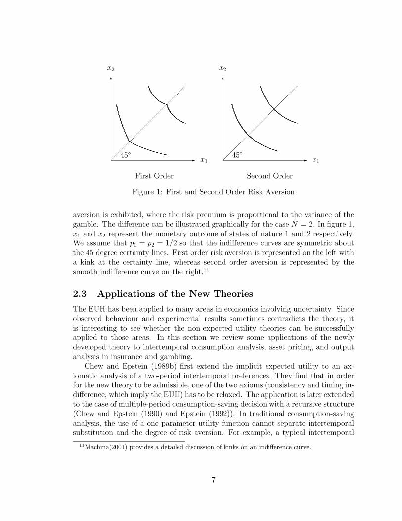
Figure 1: First and Second Order Risk Aversion

aversion is exhibited, where the risk premium is proportional to the variance of thegamble. The difference can be illustrated graphically for the case N = 2. In figure 1,x1 and x2 represent the monetary outcome of states of nature 1 and 2 respectively.We assume that p1 = p2 = 1/2 so that the indifference curves are symmetric aboutthe 45 degree certainty lines. First order risk aversion is represented on the left witha kink at the certainty line, whereas second order aversion is represented by thesmooth indifference curve on the right.11

2.3 Applications of the New Theories

The EUH has been applied to many areas in economics involving uncertainty. Sinceobserved behaviour and experimental results sometimes contradicts the theory, itis interesting to see whether the non-expected utility theories can be successfullyapplied to those areas. In this section we review some applications of the newlydeveloped theory to intertemporal consumption analysis, asset pricing, and outputanalysis in insurance and gambling.

Chew and Epstein (1989b) first extend the implicit expected utility to an ax-iomatic analysis of a two-period intertemporal preferences. They find that in orderfor the new theory to be admissible, one of the two axioms (consistency and timing in-difference, which imply the EUH) has to be relaxed. The application is later extendedto the case of multiple-period consumption-saving decision with a recursive structure(Chew and Epstein (1990) and Epstein (1992)). In traditional consumption-savinganalysis, the use of a one parameter utility function cannot separate intertemporalsubstitution and the degree of risk aversion. For example, a typical intertemporal

11Machina(2001) provides a detailed discussion of kinks on an indifference curve.

7

utility function is

U(c0, p) = f(c0) + βE

∞∑t=1

βt−1f(ct)

and

f(c) =

{c1−α/(1− α), 0 < α 6= 1log c, α = 1

where ct is the consumption expenditure in period t, t = 0, 1, . . . ,∞, p is the probabil-ity measure of the future (uncertain) consumption vector (c1, c2, . . .), and β ∈ (0, 1)is the discount factor. Here α serves both as a relative risk aversion parameter andthe reciprocal of the elasticity of substitution. By modifying the recursivity axiom,Chew and Epstein (1990) show that the two conceptions can be untangled by aclass of utility functions that exhibits first order risk aversion, for example, the onesuggested by Yaari (1987, p. 113). If the recursivity axiom is not assumed, however,then preferences may be inconsistent; that is, a consumption plan formulated att = 0 may not be pursued in subsequent periods. The situation can be modelled asa non-cooperative game between the decision maker at different times and a perfectNash equilibrium is taken to describe the behaviour.

Using a similar approach, Epstein and Zin (1989) develop a generalized intertem-poral capital asset pricing model (CAPM). This model is used to study the equitypremium puzzle in the U.S., which has a historical average value of 6.2%. Using cal-ibration of preferences by simulation technique, empirical results by Epstein and Zin(1990) show that the use of non-expected utility function can explain at least a part(2%) of the equity premium. Epstein and Zin (1991) also apply the intertemporalCAPM to update the permanent income hypothesis of Hall (1978). In this study theutility function takes the form

Ut = W (ct, µ[Ut+1|It])

where µ is the certainty equivalent of the recursive utility Ut+1 at period t + 1 giventhe information It in period t. The separation of intertemporal substitution and riskaversion makes the model more realistic. The resulting estimating equation is theweighted sum of two factors: a relation between consumption growth and asset return(intertemporal CAPM), and a relation between the risk of a particular asset withthe return of the market portfolio (static CAPM). They conclude that the expectedutility hypothesis is rejected, but the performance of the non-expected utility modelis sensitive to the choice of the consumption measure (non-durable goods, durable,services, etc.). Average elasticity of substitution is less than one and average relativerisk aversion is close to one.

Using the implicit utility function as described in (5), Diewert (1993, 1995) out-lines simple models for measuring the real outputs of the insurance and gamblingsectors. Here we describe the model of a two-state lottery game. This simple model

8

will be extended in the next section into a six-state lottery. The two-state lottery isL = (p1, p2), with p2 = 1− p1. The corresponding outcomes are

x1 = y − w, x2 = y + Rw (7)

where y is the consumer’s income, w is the wager, and R is the payout ratio. As-suming homothetic preferences, the implicit utility function φu can be written as γin (6):

φu(z) = γ(z/u).

In order to provide a kink in the indifference curve, we employ the following func-tional form for γ:

γ(z) =

{α + (1− α)zβ, z ≥ 11− α + αzβ, z < 1

(8)

where 0 < α < 1/2, β < 1, β 6= 0. The implicit expected utility in (5) for this gameis

p1φu(x1) + p2φu(x2)− φu(u) = 0. (9)

Substituting γ in (8) into (9) as φu, we have, for x1 < x2,

u = [δxβ1 + (1− δ)xβ

2 ]1/β (10)

where δ ≡ p1α/[p1 + (1 − p1)(1 − α)]. Putting (7) into (10), the consumer’s utilitymaximization problem is

maxw

[δ(y − w)β + (1− δ)(y + Rw)β]1/β

where 0 ≤ w ≤ y. The first order condition is

y + Rw∗

y − w∗ =

[1− δ

δR

] 11−β

=

[(1− p1)(1− α)R

p1α

] 11−β

≡ b.

Solving for the optimal w∗ we have

w∗ =y(b− 1)

b + R.

Since y, R, and w∗ are observable, we can calculate b in each period. Then α andβ can be estimated with a regression model. Having estimated α and β, we cancalculate the consumer’s utility level without gambling:

u0 = [δyβ + (1− δ)yβ]1/β = y.

9

Similarly, the utility level with gambling is

u∗ = [δ(y − w)β + (1− δ)(y + Rw)β]1/β.

The real output of the gambling service is then

Q = u∗ − u0.

3 Modelling the Gambling Sector

3.1 Gambling Sectors in Canada

The gambling industry in Canada has been growing in size and in revenue over thelast decade. For example, revenue increased from $2.7 billion in 1992 to $7.4 billionin 1998, while employment grew from 11,900 from 1992 to 39,200 in 1999. In 1992,government lotteries were the major component in all games of chances, representing90% of all gambling returns. They peaked at $2.8 billion and have been declining at amoderate rate. On the other hand, video lottery terminals (VLTs) and casinos havegrown rapidly. In 1998 revenue from the latter has overtaken government lotteriesas the dominant player (Marshall, 2000).

Government lotteries are administered by five regional crown corporations, namely,Atlantic Lottery Corporation, Loto-Quebec, Ontario Lottery and Gaming Corpora-tion, Western Canada Lottery Corporation, and British Columbia Lottery Corpora-tion. Most of these corporations offer their own local lottery games. The nationalgames, Lotto 6/49, Celebration (a special event lottery), and Super 7, however,are shared by all the corporations through the coordination of the Canadian In-terprovincial Lottery Corporation, which was established in 1976 to operate jointlottery games across Canada. Lotto 6/49 games are held twice a week on Wednes-day and Saturday. Forty five percent of the sales revenue goes to the prize fund. Thefifth prize, which requires matching three numbers out of the six drawn, has a fixedprize of $10. The prize fund, after subtracting the payout for all the fifth prizes,becomes the pool fund. This pool fund is divided among the other prizes by fixedshares as shown in Table 1. The prize money is shared equally among the winnersof a particular prize category. If there is no winner for the jackpot, the prize moneywill be accumulated (rollover) to the prize fund of the next draw. About 13.3% ofthe sales revenue is used as the administration and retailing costs. This portion isused by Statistics Canada as the output the Lotto 6/49 game in the GDP.

3.2 The Output of Government Lotteries

In this section we extend Diewert’s (1995) simple model to the measurement problemof a common lottery sector. A typical game of lottery, for example Lotto 6/49 in

10

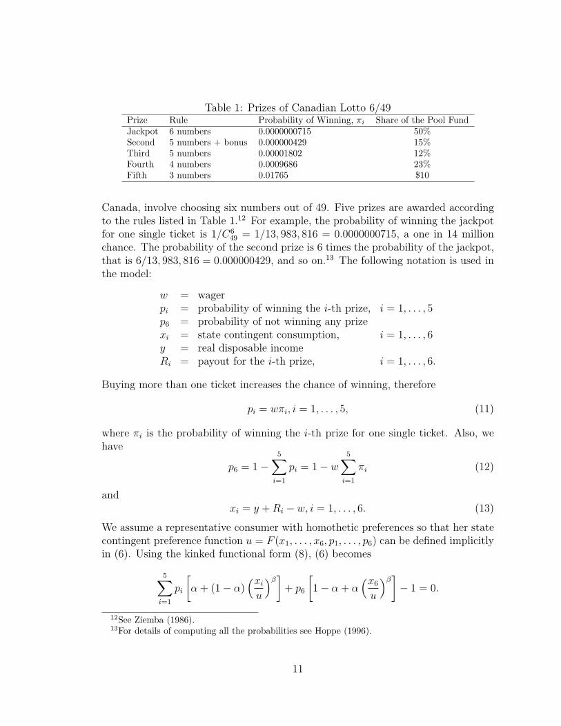
Table 1: Prizes of Canadian Lotto 6/49Prize Rule Probability of Winning, πi Share of the Pool FundJackpot 6 numbers 0.0000000715 50%Second 5 numbers + bonus 0.000000429 15%Third 5 numbers 0.00001802 12%Fourth 4 numbers 0.0009686 23%Fifth 3 numbers 0.01765 $10

Canada, involve choosing six numbers out of 49. Five prizes are awarded accordingto the rules listed in Table 1.12 For example, the probability of winning the jackpotfor one single ticket is 1/C6

49 = 1/13, 983, 816 = 0.0000000715, a one in 14 millionchance. The probability of the second prize is 6 times the probability of the jackpot,that is 6/13, 983, 816 = 0.000000429, and so on.13 The following notation is used inthe model:

w = wagerpi = probability of winning the i-th prize, i = 1, . . . , 5p6 = probability of not winning any prizexi = state contingent consumption, i = 1, . . . , 6y = real disposable incomeRi = payout for the i-th prize, i = 1, . . . , 6.

Buying more than one ticket increases the chance of winning, therefore

pi = wπi, i = 1, . . . , 5, (11)

where πi is the probability of winning the i-th prize for one single ticket. Also, wehave

p6 = 1−5∑

i=1

pi = 1− w5∑

i=1

πi (12)

andxi = y + Ri − w, i = 1, . . . , 6. (13)

We assume a representative consumer with homothetic preferences so that her statecontingent preference function u = F (x1, . . . , x6, p1, . . . , p6) can be defined implicitlyin (6). Using the kinked functional form (8), (6) becomes

5∑i=1

pi

[α + (1− α)

(xi

u

)β]

+ p6

[1− α + α

(x6

u

)β]− 1 = 0.

12See Ziemba (1986).13For details of computing all the probabilities see Hoppe (1996).

11

Solving for u and using (11), (12), and (13), we have

u(w) =

[(1− α)w

∑5i=1 πi(y + Ri − w)β + α

(1− w

∑5i=1 πi

)(y − w)β

α + (1− 2α)w∑5

i=1 πi

]1/β

(14)

The consumer’s utility maximization problem is to maximize u(w) subject to theconstraint 0 ≤ w ≤ y. For notational convenience, we define the following variablesas

d = y − w

p =∑5

i=1 πi

q =∑5

i=1 πi(y + Ri − w)β−1

r =∑5

i=1 πi(y + Ri − w)β

(15)

The first order condition can be written as

α(1−α)r−βq(1−α)[α+(1−2α)wp]w−αβ(1−wp)[α+(1−2α)wp]dβ−1−α(1−α)pdβ = 0.

Rearranging terms we get a quadratic equation in w:

[βp(α(1−2α)pdβ−1−(1−α)(1−2α)2q)]w2+[αβ(αpdβ−1−(1−α)q−(1−2α)pdβ−1)]w

+ α[(1− α)r − αβdβ−1 − (1− α)pdβ] = 0.

Solving for this quadratic equation give us the optimal level of wager:

w∗ ={−αβ(αpdβ−1 − (1− α)q − (1− 2α)pdβ−1)

±[{αβ(αpdβ−1 − (1− α)q − (1− 2α)pdβ−1)}2 −

4α[(1− α)r − αβdβ−1 − (1− α)pdβ]

[βp(α(1− 2α)pdβ−1 − (1− α)(1− 2α)q)]]1/2

}/2

{βp(α(1− 2α)pdβ−1 − (1− α)(1− 2α)q)

}(16)

Equation (16) is the estimation equation for the parameters α and β, given the datain the other variables. Notice that w appears in the right hand side of the equationthrough (15). But the effects of w on d, q, and r are negligible since the disposableincome y and the sum of y and payout prizes Ri are much larger than w. Anotherfunctional form, the kinked quadratic generating function

γ(z) =

{z + α(z − 1) + β(z − 1)2, z ≥ 1z, z < 1

was attempted in addition to (8) but the analysis yielded no explicit solution for w.The output of services provided by Lotto 6/49 is equal to the difference between

utility level with the lotteries and utility without lottery using (14), ie,

Qt = u(wt)− u(0) (17)

12

0

50

100

150

200

250

01/98 07/98 01/99 07/99 01/00 07/00 01/01 07/01

Million $

Period

bb b b b

bb b b b b b b b b b b b b b b b b b b b b

bb b b

b b b bb b b b b b b b b

b b b b

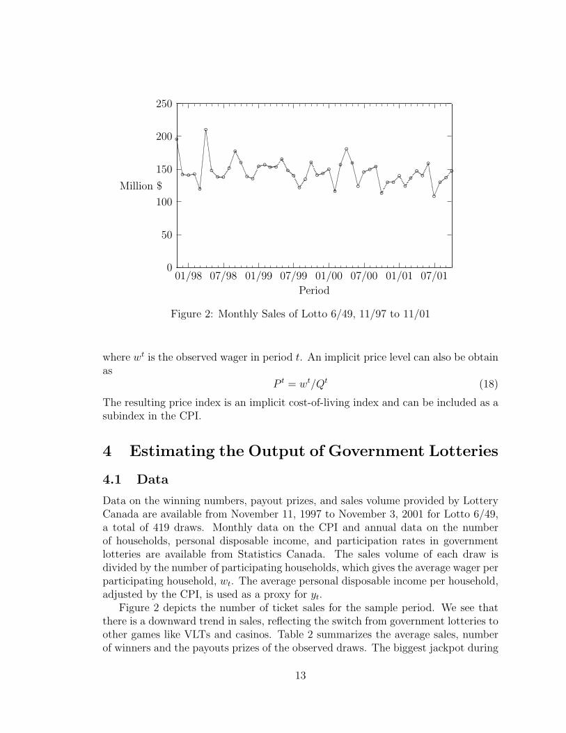
Figure 2: Monthly Sales of Lotto 6/49, 11/97 to 11/01

where wt is the observed wager in period t. An implicit price level can also be obtainas

P t = wt/Qt (18)

The resulting price index is an implicit cost-of-living index and can be included as asubindex in the CPI.

4 Estimating the Output of Government Lotteries

4.1 Data

Data on the winning numbers, payout prizes, and sales volume provided by LotteryCanada are available from November 11, 1997 to November 3, 2001 for Lotto 6/49,a total of 419 draws. Monthly data on the CPI and annual data on the numberof households, personal disposable income, and participation rates in governmentlotteries are available from Statistics Canada. The sales volume of each draw isdivided by the number of participating households, which gives the average wager perparticipating household, wt. The average personal disposable income per household,adjusted by the CPI, is used as a proxy for yt.

Figure 2 depicts the number of ticket sales for the sample period. We see thatthere is a downward trend in sales, reflecting the switch from government lotteries toother games like VLTs and casinos. Table 2 summarizes the average sales, numberof winners and the payouts prizes of the observed draws. The biggest jackpot during

13

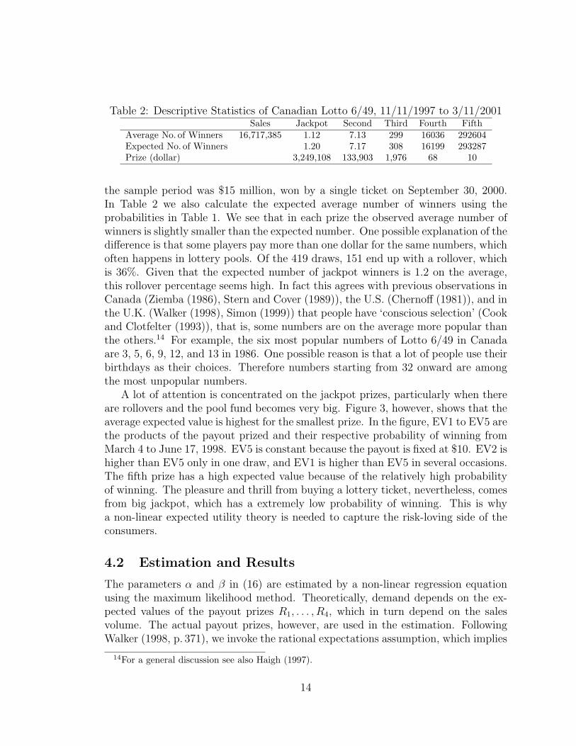
Table 2: Descriptive Statistics of Canadian Lotto 6/49, 11/11/1997 to 3/11/2001Sales Jackpot Second Third Fourth Fifth

Average No. of Winners 16,717,385 1.12 7.13 299 16036 292604Expected No. of Winners 1.20 7.17 308 16199 293287Prize (dollar) 3,249,108 133,903 1,976 68 10

the sample period was $15 million, won by a single ticket on September 30, 2000.In Table 2 we also calculate the expected average number of winners using theprobabilities in Table 1. We see that in each prize the observed average number ofwinners is slightly smaller than the expected number. One possible explanation of thedifference is that some players pay more than one dollar for the same numbers, whichoften happens in lottery pools. Of the 419 draws, 151 end up with a rollover, whichis 36%. Given that the expected number of jackpot winners is 1.2 on the average,this rollover percentage seems high. In fact this agrees with previous observations inCanada (Ziemba (1986), Stern and Cover (1989)), the U.S. (Chernoff (1981)), and inthe U.K. (Walker (1998), Simon (1999)) that people have ‘conscious selection’ (Cookand Clotfelter (1993)), that is, some numbers are on the average more popular thanthe others.14 For example, the six most popular numbers of Lotto 6/49 in Canadaare 3, 5, 6, 9, 12, and 13 in 1986. One possible reason is that a lot of people use theirbirthdays as their choices. Therefore numbers starting from 32 onward are amongthe most unpopular numbers.

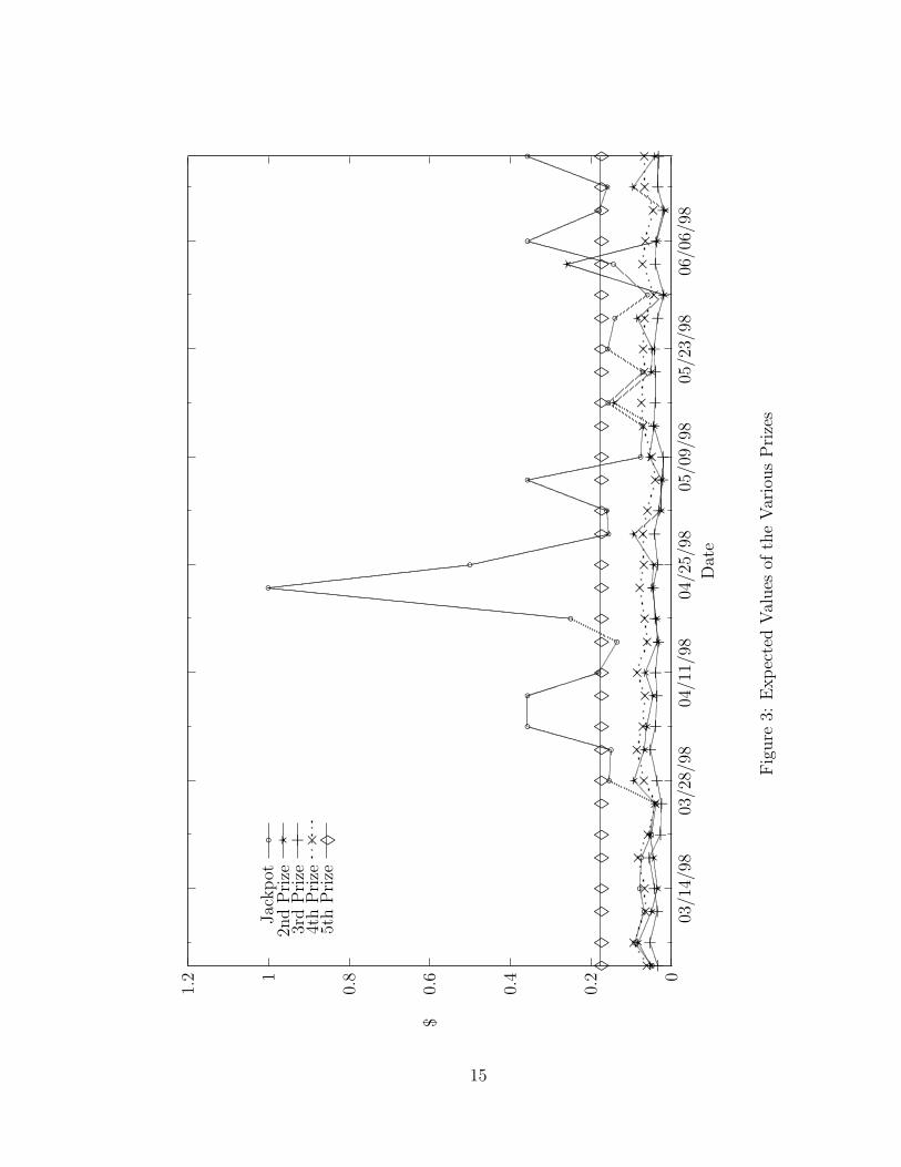
A lot of attention is concentrated on the jackpot prizes, particularly when thereare rollovers and the pool fund becomes very big. Figure 3, however, shows that theaverage expected value is highest for the smallest prize. In the figure, EV1 to EV5 arethe products of the payout prized and their respective probability of winning fromMarch 4 to June 17, 1998. EV5 is constant because the payout is fixed at $10. EV2 ishigher than EV5 only in one draw, and EV1 is higher than EV5 in several occasions.The fifth prize has a high expected value because of the relatively high probabilityof winning. The pleasure and thrill from buying a lottery ticket, nevertheless, comesfrom big jackpot, which has a extremely low probability of winning. This is whya non-linear expected utility theory is needed to capture the risk-loving side of theconsumers.

4.2 Estimation and Results

The parameters α and β in (16) are estimated by a non-linear regression equationusing the maximum likelihood method. Theoretically, demand depends on the ex-pected values of the payout prizes R1, . . . , R4, which in turn depend on the salesvolume. The actual payout prizes, however, are used in the estimation. FollowingWalker (1998, p. 371), we invoke the rational expectations assumption, which implies

14For a general discussion see also Haigh (1997).

14

0

0.2

0.4

0.6

0.81

1.2

03/1

4/98

03/2

8/98

04/1

1/98

04/2

5/98

05/0

9/98

05/2

3/98

06/0

6/98

$

Dat

e

Jac

kpot

bbbb

b bbb

bbb b

bb

b b

bb

b bbb

bbb b

bbb b

b

b2n

dP

rize

??

??

??

??

??

??

??

??

?

??

??

?

??

?

?

?

??

??

?3r

dP

rize

++

++

++

++

++

++

++

++

++

++

++

++

++

++

++

+

+4t

hP

rize

××

××

××

××

××

××

××

××

××

××

××

××

××

××

××

×

×5t

hP

rize

♦♦

♦♦

♦♦

♦♦

♦♦

♦♦

♦♦

♦♦

♦♦

♦♦

♦♦

♦♦

♦♦

♦♦

♦♦

♦

♦

Fig

ure

3:E

xpec

ted

Val

ues

ofth

eVar

ious

Pri

zes

15

10

15

20

25

30

35

40

45

50

0.2 0.4 0.6 0.8 1 1.2 1.4

Sales

Expected value of a ticket, $

Sales in million $

bb

bbb

bb

bb bbb bbb bb bb bb bb bb bbbbbbb b b

b

b bbb bbb bbb

bbbb

b

b

bb bb b bb bbb bb

bb bbbbb b bbbbb bb bb b bbb b b

b

bb

bb

bb

bb

bb

bb bb

bbb bb b bb b

b

b bb bbbbbbbb b b

b

b b bb

b bb

b bb

b b bb

b b bbbb b bb

b bb b b bb

bb

bb b bbb bb b bb b bb

b b bb b bb bb b bb

b bb bb bb b bb bbbb b b b

b b

b bb b bbb bb

bb bbb b b

bbb b bb bb bb

bb bbb bb b bb b bb b bb b b

b bb bbb b

bb bb b

b bb

b bb

b

bbbb bb

b bb bb bb b bb

b b bb

bb b b bb b

bb b bb bb b bb b

bb

b b bbbb b b bb b bb bbb bb

b b bb b bbb b bb bb bb

b bb

bb bbbb bb bb bbbb bbb

b bb

bb bbb

bb b b b bb bb b b b bb

b b bbbb b bb b bbb bb

bbbbb bb bb b bb

b b bb bbb b bb b b

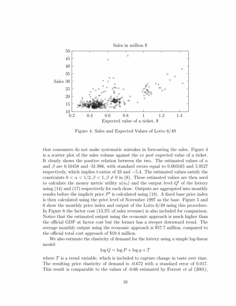
Figure 4: Sales and Expected Values of Lotto 6/49

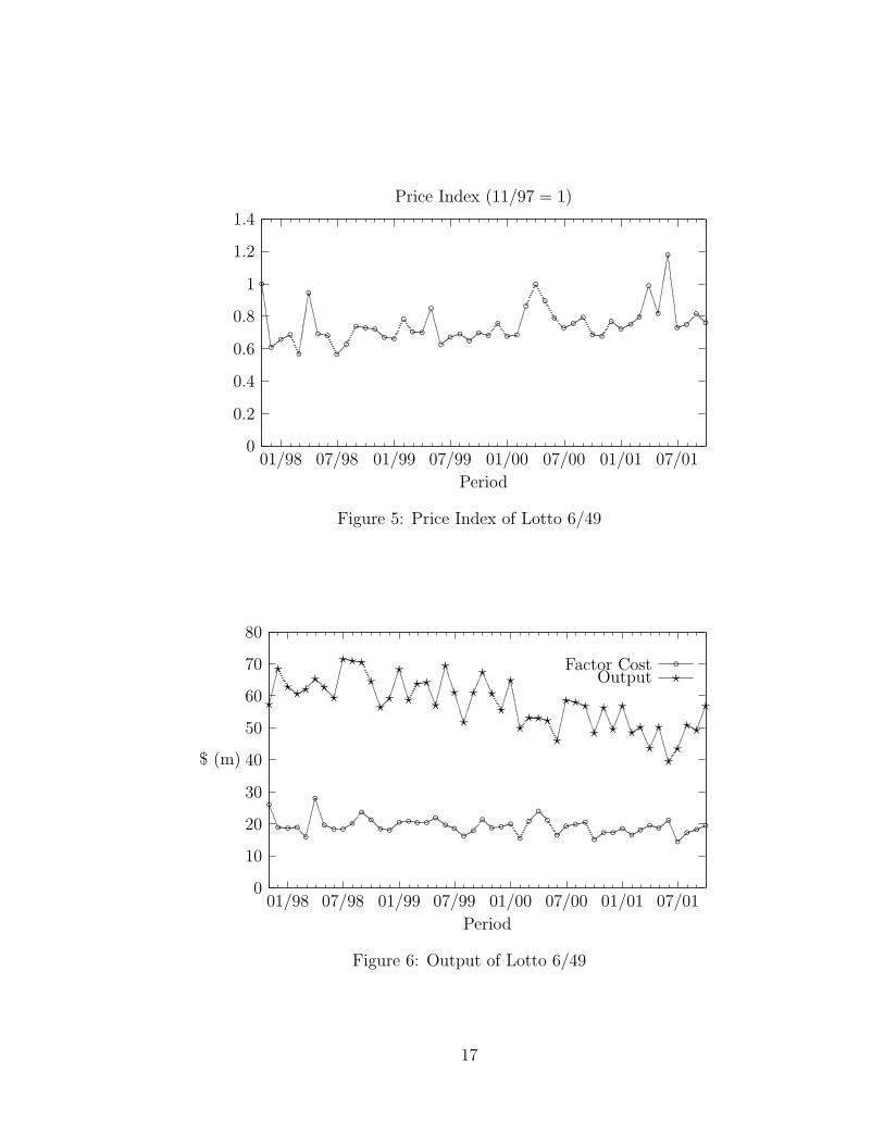
that consumers do not make systematic mistakes in forecasting the sales. Figure 4is a scatter plot of the sales volume against the ex post expected value of a ticket.It clearly shows the positive relation between the two. The estimated values of αand β are 0.10458 and -31.986, with standard errors equal to 0.003165 and 5.9527respectively, which implies t-ratios of 33 and −5.4. The estimated values satisfy theconstraints 0 < α < 1/2, β < 1, β 6= 0 in (8). These estimated values are then usedto calculate the money metric utility u(wt) and the output level Qt of the lotteryusing (14) and (17) respectively for each draw. Outputs are aggregated into monthlyresults before the implicit price P t is calculated using (18). A fixed base price indexis then calculated using the price level of November 1997 as the base. Figure 5 and6 show the monthly price index and output of the Lotto 6/49 using this procedure.In Figure 6 the factor cost (13.3% of sales revenue) is also included for comparison.Notice that the estimated output using the economic approach is much higher thanthe official GDP at factor cost but the former has a steeper downward trend. Theaverage monthly output using the economic approach is $57.7 million, compared tothe official total cost approach of $19.4 million.

We also estimate the elasticity of demand for the lottery using a simple log-linearmodel:

log Q = log P + log y + T

where T is a trend variable, which is included to capture change in taste over time.The resulting price elasticity of demand is -0.672 with a standard error of 0.017.This result is comparable to the values of -0.66 estimated by Forrest et al (2001),

16

0

0.2

0.4

0.6

0.8

1

1.2

1.4

01/98 07/98 01/99 07/99 01/00 07/00 01/01 07/01

Period

Price Index (11/97 = 1)

bb b b b

bb b b b b b b b b b b b b

b b b b b b b b b b b b b b b b b b b b b bb b

b

b b b b

Figure 5: Price Index of Lotto 6/49

0

10

20

30

40

50

60

70

80

01/98 07/98 01/99 07/99 01/00 07/00 01/01 07/01

$ (m)

Period

Factor Cost

b b b b bb b b b b b b b b b b b b b b b b b b b b b b b b b b b b b b b b b b b b b b b b b b

bOutput

?

????

???

????

??

?

???

?

?

?

?

????

?

????

?

???

?

??

?

????

??

??

?

?

Figure 6: Output of Lotto 6/49

17

who use a two-stage OLS estimation with the difference between the ticket priceand the expected value as the effective price of lottery. Using a similar approach,Gully and Scott (1993) estimated the price elasticities of four state-operated lottosin the U.S., with results ranging from -0.40 to -2.5. Farrell and Walker (1999) usedcross-sectional data to study the demand for lottery in the U.K. using the Heckmanselection model. Their estimated price elasticity was -0.763. Also, Beenstock andHaitovsky (2001) study the demand for lotto in Israel using time series data, withthe estimated long-run price elasticity equal to -0.65. It is surprising that theseresults, although differing in methods, nature of data, and countries, show very closeestimates of price elasticities of demand.

5 Conclusion

The classical expected utility hypothesis fails to capture a consumer’s risk aversebehaviour in facing big losses with small probabilities and the risk loving behaviourinvolving large gain with small probability. New non-expected utility theories havebeen developed to overcome the difficulty. In this paper we have applied the implicitexpected utility theory to the problem of measuring outputs of lotteries. The resultsshow that output levels of Lotto 6/49 in Canada is almost three times higher than theofficial statistics, which uses the total cost of providing the service approach as outputmeasurement principle. This kind of direct economic approach is recommendedby SNA93 for government and non-profit organization output measurement. Themethod developed here can be potentially applied to other games of chance.15 Theestimated price elasticity of demand for lottery in Canada is close to that of the U.K.and Israel in previous studies.

References

Allais, M. (1953) ‘Le Comportement de L’homme Rationnel Devant le Risque: Cri-tique des Postulats et Axiomes de L’ecole Americaine,’ Econometrica, Vol. 21,No. 4, 503-546.

Arrow, K.J. (1964) ‘The Role of Securities in the Optimal Allocation of Risk-bearing,’Review of Economic Studies, Vol. 31, No. 2, 91-96.

Beenstock, Michael and Yoel Haitovsky (2001) ‘Lottomania and other anomalies inthe market for lotto,’ Journal of Economic Psychology, 22, 721-744.

Blackorby, Charles, Russel Davidson, and David Donaldson (1977) ‘A homiletic Ex-position of the Expected Utility Hypothesis,’ Economica, 44, 351-358.

15See Dubins and Savage (1965) and Richard Epstein (1977) for the mathematical analysis of awhole variety of games.

18

Chernoff, Herman (1981) ‘How to Beat the Massachusetts Numbers Game,’ Mathe-matical Intelligencer, Vol. 3, No. 4, 166-172.

Chew, Soo Hong (1983) ‘A Generalization of the Quasilinear Mean with Applica-tions to the Measurement of Income Inequality and Decision Theory Resolvingthe Allais Paradox,’ Econometrica, Vol. 51, No. 4, 1065-1092.

Chew, S.H. and L.G. Epstein (1989a) ‘A Unifying Approach to Axiomatic Non-expectedUtility Theories,’ Journal of Economic Theory, 49, 207-240.

Chew, S.H. and Larry G.Epstein (1989b) ‘The Structure of Preferences and Atti-tudes towards the Timing of the Resolution of Uncertainty,’ International Eco-nomic Review, Vol. 30, No. 1, 103-117.

Chew, Soo Hong and Larry G.Epstein (1990) ‘Nonexpected Utility Preferences in aTemporal Framework with an Application to Consumption-Savings Behaviour,’Journal of Economic Theory, 50, 54-81.

Cook, Philip J. and Charles T. Clotfelter (1993) ‘The Peculiar Scale Economies ofLotto,’ American Economic Review, Vol. 83, No. 3, 634-643.

Cox, James C. and Vjollca Sadiraj (2002) ‘Risk Aversion and Expected Utility The-ory: Coherence for Small- and Large-Stakes Gambles,’Mimeo, University ofArizona.

Debreu, Gerard (1959) Theory of Value, New Haven: Yale University Press.

Dekel, Eddie (1986) ‘An Axiomatic Characterization of Preferences under Uncer-tainty: Weakening the Independence Axiom,’ Journal of Economic Theory,40, 304-318.

Diecidue, Enrico and Peter P.Wakker (2001) ‘On the Intuition of Rank-DependentUtility,’ Journal of Risk and Uncertainty, 23:3, 281-298.

Diewert, W.E. (1993) ‘Symmetric Means and Choice under Uncertainty,’ in W.E.Diewert and A.O. Nakamura, eds, Essays in Index Number Theory, Vol. 1,Amsterdam: North-Holland, 335-433.

Diewert, W. Erwin (1995) ‘Functional Form Problems in Modeling Insurance andGambling,’ Geneva Papers on Risk and Insurance Theory, 20, 135-150.

Dubins, Lester E. and Leonard J. Savage (1965) How to Gamble If You Must, NewYork: McGraw-Hill Book Co.

19

Epstein, Larry G. (1992) ‘Behavior under Risk: Recent Developments in Theoryand Applications,’ in Jean-Jacques Laffont, ed, Advances in Economic Theory,Sixth World Congress, Vol. II, Cambridge: Cambridge University Press, 1-63.

Epstein, Larry G. and Stanley E. Zin (1989) ‘Substitution, Risk Aversion, and theTemporal Behavior of Consumption and Asset Returns: A Theoretical Frame-work,’ Econometrica, Vol. 57, No. 4, 937-969.

Epstein, Larry G. and Stanley E. Zin (1990) ‘First-Order Risk Aversion and the Eq-uity Premium Puzzle,’ Journal of Monetary Economics, 26, 387-407.

Epstein, Larry G. and Stanley E. Zin (1991) ‘Substitution, Risk Aversion, and theTemporal Behavior of Consumption and Asset Returns: An Empirical Analy-sis,’ Journal of Political Economy, Vol. 99, No. 2, 263-286.

Epstein, Richard A (1977) The Theory of Gambling and Statistical Logic, New Yorker:Academic Press.

Farrell, Lisa and Ian Walker (1999) ‘The Welfare Effects of Lotto: Evidence fromthe UK,’ Journal of Public Economics, 72, 99-120.

Forrest, David, O. David Gulley, and Robert Simmons (2000) ‘Elasticity of Demandfor UK National Lottery Tickets,’ National Tax Journal, Vol. LIII, No. 4, Part1, 853-863.

Friedman, Milton and L. J. Savage (1948) ‘The Utility Analysis of Choices InvolvingRisk,’ Journal of Political Economy, Vol. LVI, No. 4, 279-304.

Gorman, W.M. (1968) ‘The Structure of Utility Functions,’ Review of EconomicStudies, Vol. 35, No. 4, 367-390.

Gul, Faruk (1991) ‘A Theory of Disappointment Aversion,’ Econometrica, Vol. 59,No. 3, 667-686.

Gulley, O. David and Frank A. Scott, Jr. (1993) ‘The Demand for Wagering on State-Operated Lotto Games,’ National Tax Journal, Vol. 45, No. 1, 13-22.

Haigh, John (1997) ‘The Statistics of the National Lottery,’ Journal of the RoyalStatistical Society, A, 160, Part 2, 187-206.

Hall, Robert E. (1978) ‘Stochastic Implications of the Life Cycle-Permanent IncomeHypothesis: Theory and Evidence,’ Journal of Political Economy, Vol. 86,No. 6, 971-987.

20

Hoppe, Fred M. (1996) ‘Mathematical Appendix to the Maclean’s Magazine articleby John Schofield, November 4, 1996,’ Department of Mathematics, McMasterUniversity, http://www.math.mcmaster.ca/fred/Lotto/.

Inter-Secretariat Working Group on National Accounts (1993) System of National Ac-counts 1993, Commission of the European Communities, IMF, OECD, UN,World Bank.

Kahneman, Daniel and Amos Tversky (1979) ‘Prospect Theory: An Analysis of De-cisions under Risk,’ Econometrica, Vol. 47, No. 2, 263-291.

Luce, R.Duncan and Howard Raiffa (1957) Games and Decisions, 1985 Dover Edi-tion.

Machina, Mark J. (1982) “‘Expected Utility” Analysis without the IndependenceAxiom,’ Econometrica, Vol. 50, No. 2, 277-323.

Machina, Mark J. (1997) ‘Choice under Uncertainty: Problems Solved and Unsolved,’in Partha Dasgupta and Karl-Goran Maler, eds, The Environment and Emerg-ing Development Issues, Vol. 1, Oxford: Clarendon Press, 201-255.

Machina, Mark J. (2001) ‘Payoff Kinks in Preferences over Lotteries,’ Journal ofRisk and Uncertainty, 23:3, 207-260.

Marshall, Katherine (1998) ‘The gambling industry: Raising the stakes’, ServicesIndicators, Statistics Canada, 4th Quarter, 29-38.

Marshall, Katherine (2000) ‘Update on Gambling,’ Perspectives, Statistics Canada,Spring, 29-35.

Pratt, John W., Howard Raiffa, and Robert Schlaifer (1995) Introduction to Statis-tical Decision Theory, Cambridge: The MIT Press.

Quiggin, John (1993) Generalized Expected Utility Theory: The Rank-DependentModel, Norwell: Kluwer Academic.

Rabin, Matthew (2000) ‘Risk Aversion and Expected-Utility Theory: A CalibrationTheorem,’ Econometrica, Vol. 68, No. 5, 1281-1292.

Rabin, Matthew and Richard H.Thaler (2001) ‘Risk Aversion,’ Journal of EconomicPerspectives, Vol. 15, No. 1, 219-232.

Samuelson, Paul A. (1952) ‘Probability, Utility, and the Independence Axiom,’ Econo-metrica, 20, 670-678.

21

Segal, Uzi and Avia Spivak (1990) ‘First Order versus Second Order Risk Aversion,’Journal of Economic Theory, 51, 111-125.

Simon, Jonathan (1999) ‘An Analysis of the Distribution of Combinations Chosenby UK National Lottery Players,’ Journal of Risk and Uncertainty, 17:3, 243-276.

Starmer, Chris (2000) ‘Developments in Non-Expected Utility Theory: The Huntfor a Descriptive Theory of Choice under Risk,’ Journal of Economic Literature,Vol. XXXVIII, No. 2, 332-382.

Stern, Hal and Thomas M. Cover (1989) ‘Maximum Entropy and the Lottery,’ Jour-nal of the American Statistical Association, Vol. 84, No. 408, 980-985.

von Neumann, John and Oskar Morgenstern (1953) Theory of Games and EconomicBehavior, Princeton: Princeton University Press.

Walker, Ian (1998) ‘The Economic Analysis of Lotteries,’ Economic Policy, October,359-401.

Watt, Richard (2002) ‘Defending Expected Utility Theory,’ Journal of EconomicPerspectives, 16:2, 227-230.

Yaari, Menahem E. (1987) ‘The Dual Theory of Choice under Risk,’ Econometrica,Vol. 55, No. 1, 95-115.

Ziemba, William T. (1986) Dr Z’s 6/49 Lotto Guidebook, Vancouver: Dr. Z Invest-ments Inc.

22