Measuring the Likelihood of Small Business Loan Default:

Community Development Financial Institutions (CDFIs) and the use of

Credit-Scoring to Minimize Default Risk1

Andrea Ruth Coravos

Professor Charles Becker, Faculty Advisor

Duke University

Durham, North Carolina

2010

1 Honors thesis submitted in partial fulfillment of the requirements for Graduation with Distinction in Economics in Trinity

College of Duke University. The data and methodology in this paper have been certified by the Institutional Review Board (IRB).

2

Abstract

Community development financial institutions (CDFIs) provide financial services to

underserved markets and populations. Using small business loan portfolio data from a national

CDFI, this paper identifies the specific borrower, lender, and loan characteristics and changes in

economic conditions that increase the likelihood of default. These results lay the foundation for

an in-house credit-scoring model, which could decrease the CDFI’s underwriting costs while

maintaining their social mission. Credit-scoring models help CDFIs quantify their risk, which

often allows them to extend more credit in the small business community.*

*I am grateful to Professor Charles Becker for his year-long encouragement and advice. I would

like to thank X CDFI for providing the data and incredible support for this project. My thesis

Professors Kent Kimbrough and Michelle Connolly substantially shaped the models in this

thesis. I would have not been able to write such an in-depth statistical analysis without the help

of Kofi Acquah and the members of GIS Services in Perkins Library. My peers in the Economics

Workshops 198 and 199 provided great support all year. Thank you to Professor Lori Leachman

for granting the Research in Practice Program funding for this work.

3

Measuring the Likelihood of Small Business Loan Default:

CDFIs and the use of Credit-Scoring to Minimize Default Risk

I. Introduction

Community development financial institutions (CDFIs) provide financial services to

underserved markets and populations. In theory, credit needs would be appropriately priced in a

perfectly competitive market, but in reality, many businesses and consumers may not be served

effectively by traditional institutions due to high transaction costs and asymmetric information.

To counter this problem, CDFIs extend more credit to “mission” borrowers, usually consisting of

women, minorities, and/or low-wealth individuals. The first CDFIs were created out of the

Johnson Administration’s “War on Poverty Campaign” in the 1960s and 1970s. Now, CDFI

investors come from a broad range of backgrounds, and some are lured to CDFIs purely for their

expected returns rather than for a social purpose. As CDFIs in the United States expand to larger

and more competitive markets, many want to better manage the risk in their portfolios.

CDFIs offer a range of financial services, covering both residential and commercial

loans, for economically disadvantaged communities. The data in this paper are from X CDFI,

which is one of the largest CDFIs in the United States.2 Using their portfolio, I identify the

characteristics associated with SBL repayment. Building on an internal study at X, I isolate the

borrower, lender, loan and macroeconomic characteristics that affect the likelihood of default.

These results lay the foundations for an in-house credit-scoring model, which has the potential to

increase consistency and reduce the costs of underwriting a loan. Credit-scoring models allow

banks to quantify risk, which encourages better lending practices, and often extend more credit in

the small business community.

2 The CDFI has requested to keep its identity anonymous.

4

However, credit-scoring may also force the CDFI to drift away from its mission clientele

if the mission borrowers are not deemed as credit-worthy.3 CDFIs use non-traditional financial

instruments and cater to a different type of clientele compared to traditional banking institutions,

which do not face these mission borrower requirements. The current literature lacks a cohesive

body of work that identifies the characteristics of a risky loan for a CDFI-borrower population.

In addition, there is a lack of information concerning CDFI credit-scoring methodologies or

expected scoring outputs for a given small business loan portfolio. In part, this is because it is

rare and expensive for a CDFI to develop credit-scoring technologies.

The literature review in Section II is comprised of three parts. Section IIA of the literature

review discusses the idea that extending credit to the poor and underserved markets can be

profitable, a discovery often credited to microfinance institutions (MFIs). When lenders

underwrite loans to these markets, they often want to identify risky loan characteristics, which

are discussed in Section IIB. Section IIC explains how loan default models can be turned into

credit scores, which can improve the efficiency of small business loan origination. Credit-scoring

models help banks identify characteristics that contribute to loan defaults and weight those

characteristics according to their relative significance. Section III provides the theoretical

framework to build a credit-scoring method that minimizes loan defaults. The data in this paper

are discussed in Section IV, and the empirical specifications are laid out in Section V. Section VI

provides a working-world credit-scoring application of the model developed in Section V. The

concluding remarks are in Section VII.

3 Mission clientele, as described previously, includes women, minorities, and low-wealth individuals.

5

II. Literature Review

a. Discovering underserved markets across the world

In 1976, frustrated with the trickle-down approach to economic development,

Muhammad Yunus extended credit to the poorest of the poor as a social experiment. Yunus and

his bank Grameen, headquartered in Bangladesh, are often credited as being among the first

microfinance banks, institutions that have been able to tap into the hidden wealth of the poor

(Easton, 2005). The poorest people are often considered “unbankable,” because they do not have

characteristics of traditional borrowers, such as reliable credit histories or high levels of

collateral.

Over the past thirty years, many microfinance institutions (MFIs) have emerged across

the globe, and compared to traditional banks, many MFIs boast high repayment rates from

borrowers without formal credit histories (Morduch, 1999). Some of these rates, however, are

deceiving. Although institutions like Grameen report repayment rates averaging 97-98%,

Jonathan Morduch asserts that the relevant rate is about 92%. In addition, although Grameen

charges interest rates of 20% per year, it would have to charge around 32% in order to become

fully financially sustainable4 (Morduch, 1999). Banks often need to charge large interest rates

because small loans can be expensive to service and do not return large profits per loan.

The reason Grameen can survive even though it charges borrowers low interest rates is

because it depends on subsidies, a topic that has garnered warranted suspicion over the course of

microfinance’s increased popularity. In the United States, many CDFIs also charge low interest

4 A firm achieves profitability when its revenues are greater than its costs. A firm may be "profitable" with subsidies or grants,

but it may not be “financially sustainable” because without its subsidies or grants it would go under. Financial sustainability is a

more contentious issue in the microfinance world. Especially if the firm can depend on reliable and continuous grants and

subsidies, for instance from the government, a firm can be continually profitable without being financially sustainable.

6

rates because their loans are also subsidized by the government or socially-conscious investors.5

Some CDFIs are profitable, some are profitable because of subsidies, and some not profitable but

still carry on due to subsidies, including cross-subsidies from profitable activities, and investor

support for their “mission.”

Although many CDFI are inspired by microfinance initiatives in the developing world,

they have operational differences in the United States, which is the focus of this paper. A MFI is

a general term for an institution that provides financial services to low-income clientele who lack

access to traditional banking sources. A CDFI is an American financial institution that also

provides financial services to underserved markets. CDFIs often engage in more advanced

services than MFIs, and CDFIs are certified by the Community Development Financial

Institutions Fund at the U.S. Department of the Treasury. One prominent distinction is that a

majority of CDFIs in the U.S. do not engage in group lending as a method to minimize

asymmetric information like the MFIs in the developing world.

Gary Painter and Shui-Yan Tang (2001) study the microcredit challenge in California.

They find that most of the MFIs are not close to reaching any measure of financial

sustainability.6 They attribute part of this problem to excessive overhead costs – some of which

can be three times the size of the loan amounts. These overhead costs can include the time a loan

officer spends investigating the borrower’s background, any paperwork – both in-house and for

the government – compiled during the loan process, and other administrative tasks. They also

note that unlike in the developing world, in the U.S., an individual’s ability to obtain future credit

5 For example, many CDFIs in fact charge interest rates that are based on specific programs, rather than on the perceived risk of

the borrower. This is discussed in greater detail in the data section. 6 In this study, the MFIs were limited to institutions whose loans were $25,000 or less. The portfolios were also relatively small

and they had a relatively small underwriting team. The CDFI I am working with has a much larger range for its loans and a larger

and more sophisticated portfolio. These are significant differences.

7

is less critical for survival, because most people have the ability to fall back on the government

welfare system (Painter and Tang 2001). In other words, a CDFI-borrower population is

significantly different from an MFI’s borrowers in the developing world, and each would have a

different set of risks. The CDFI small business banks, which are designed for the low-income

entrepreneur, are also significantly different from traditional commercial banks. They develop

special relationships and localized expertise that larger banks cannot provide, which makes the

small business credit markets vast, differentiated and segmented (Ou, 2005).

b. Identifying strong borrowers versus weak ones

Because the current literature lacks a cohesive analysis of CDFI loan default

characteristics, this section identifies risky loan characteristics in populations that are similar to

CDFIs. Many institutions that service small business loans do not want or have the ability to

quantitatively track risk, due to the high costs or concern that it would compromise their mission.

All lenders do some sort of risk analysis before underwriting a loan. The two types of risk

analysis are quantitative and qualitative. Loan officers perform a qualitative risk analysis when

they interview the potential borrower, look over the business plan (if available) and review past

financial history. Quantitative risk analyses are more expensive and time consuming, because

they require keeping track of loan data both during loan origination and monitoring. Quantitative

analyses are often combined to create a “credit score,” which quantifies the predicted risk of the

borrower. Each credit-scoring model provides the best predictions when it is individually

developed for a particular bank’s loans and lending practices. This type of credit-scoring is

described in further detail in the next section.

8

The characteristics of risky loans differ between populations. This paper focuses on small

business loans, which, unlike consumer loans, generally finance investment rather than

consumption. One of the most predictive measurements of small business loan repayment is the

personal credit score. Cowan and Cowan found that the borrower’s personal credit history is

often deemed more important and predictive of repayment than the business plan or feasibility of

the idea (Cowan et al., 2006). Frame, Srinivan, and Woosley (2001) also find that the personal

consumer credit history of small business borrowers is highly predictive of loan repayment,

particularly for loans under $100,000.

Loretta Mester (1997), vice president and economist in the Research Department of the

Philadelphia Fed, cites the applicant’s monthly income, financial assets, outstanding debt,

employment tenure, homeownership, and previous loan defaults or delinquencies as predictive of

loan default for SBLs. Many CDFIs use Small Business Administration (SBA) guarantees when

they underwrite SBLs. Dennis Glennon and Peter Nigro (2005) analyze SBA loan repayment and

find that defaults are time-sensitive and are particularly affected by the changing economic

climate during the life of the loan. The probability of default in their SBA dataset peaks after six

to twelve months, which suggest that any model should include time-sensitive variables. In

addition, they find that long-term loans are more sensitive to changes in the business cycle than

short term loans. They also find that corporate structure (i.e. corporations, partnerships or sole

proprietorships) has a large influence on the odds of default. Some papers even find that lending

to better-off borrowers results in higher delinquency rates, suggesting that when borrowers have

better alternatives, they value the program less (Wenner, 1995). This shows that a selection bias

can arise if better-off borrowers go to institutions like CDFIs when they have riskier projects.

9

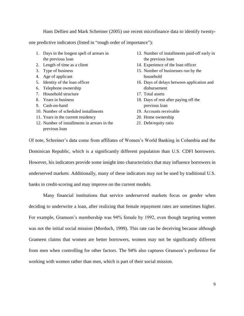
Hans Dellien and Mark Schreiner (2005) use recent microfinance data to identify twenty-

one predictive indicators (listed in “rough order of importance”):

1. Days in the longest spell of arrears in

the previous loan

2. Length of time as a client

3. Type of business

4. Age of applicant

5. Identity of the loan officer

6. Telephone ownership

7. Household structure

8. Years in business

9. Cash-on-hand

10. Number of scheduled installments

11. Years in the current residency

12. Number of installments in arrears in the

previous loan

13. Number of installments paid-off early in

the previous loan

14. Experience of the loan officer

15. Number of businesses run by the

household

16. Days of delays between application and

disbursement

17. Total assets

18. Days of rest after paying off the

previous loan

19. Accounts receivable

20. Home ownership

21. Debt/equity ratio

Of note, Schreiner’s data come from affiliates of Women’s World Banking in Columbia and the

Dominican Republic, which is a significantly different population than U.S. CDFI borrowers.

However, his indicators provide some insight into characteristics that may influence borrowers in

underserved markets. Additionally, many of these indicators may not be used by traditional U.S.

banks in credit-scoring and may improve on the current models.

Many financial institutions that service underserved markets focus on gender when

deciding to underwrite a loan, after realizing that female repayment rates are sometimes higher.

For example, Grameen’s membership was 94% female by 1992, even though targeting women

was not the initial social mission (Morduch, 1999). This rate can be deceiving because although

Grameen claims that women are better borrowers, women may not be significantly different

from men when controlling for other factors. The 94% also captures Grameen’s preference for

working with women rather than men, which is part of their social mission.

10

X has worked on an internal research project within its commercial loan portfolio. The

Kinat Report analyzes two data sets separately (SBA and non-SBA loans in X’s portfolio) with

loans that originated between 2002 and 2007. In the Small Business Administration loan (SBA)

regression, the three best predictors of loan performance are (1) personal credit score, (2) owner

management experience, and (3) length of existing business. Sixteen factors have no significant

relationships.7 I combine the same SBA and non-SBA data in this paper, supplement this dataset

with additional macroeconomic variables, and use a different method for selecting the

independent variables.

Although the popularity of microfinance in the developing world and CDFIs in the US

seems to be growing exponentially, it does not mean that they are immune to the credit bubbles

seen in other periods of economic exuberance. A recent Wall Street Journal article notes that as

more private-equity funds and other foreign investors come to invest in the tiniest loans in the

world, MFIs are having a harder time identifying qualified borrowers (Gokhale, 2009).

c. The adoption of credit-scoring technologies

After a CDFI develops a model to predict the best borrowers, the results of that model

can be turned into an in-house credit score. Credit-scoring technology is another method to

diminish the asymmetric information gap between the borrower and lender, which leads to a

more efficient allocation of capital. Credit-scoring has been more widely adopted in traditional

banks than in CDFIs, because CDFIs are concerned that they might “mission-drift away” from

7 These factors are: Loan Amount, Borrower Net Worth, Projected Breakeven at time of loan, Year, Personal Income, Use of

Proceeds, Guarantee Percentage, Personal D/I at time of loan (before X’s loan), Equity investment of business owner, SBA Type,

Personal debt-to-income at time of loan (including X’s loan), Gender, Rural/urban dummy, Type Business (Restaurant, etc), and

Race. .

11

their desired clientele if they use credit-scoring. To clarify, the term “credit-score” has two

distinctly different meanings: 8

In this paper, “credit-scoring” refers to the statistical in-house credit-scoring model rather

than the personal FICO score. Often a bank will use the borrower’s personal consumer FICO

score when deciding to underwrite the borrower’s business loan. Rarely does the bank have

access to business credit scores, especially because most of these small businesses are start-ups

or are in the early stage of development and the finances of the business are often tied with the

personal finances of the owner.

Robert Schall (2003) asserts that the use of consumer credit-scoring models could have

inherent racial or income biases because the reports are created from borrowing practices that are

more common of white and middle-class neighborhoods. Unfortunately, although this statement

could be plausible, it is difficult verify because most personal/consumer credit-scoring methods

are proprietary and confidential. In 1997, Eugene Ludwig, the U.S. Comptroller of the

Currencym warned that credit-scoring systems might be “flawed” due to the misuse of

“overrides,” which are manual approvals of a loan when the score recommends rejecting the loan

or vice versa. He claims that this can create biases that have a disproportionate impact on

8 Personal credit scores are often developed and standardized by a company, like Experian or Fair Isaac, and scores can be

purchased by a bank. Technically, the Beacon score is used by Experian, and the FICO, which stands for Fair Isaac Corporation,

was developed by Fair Isaac. The terms Beacon and FICO are often used interchangeably, although FICO has become more

commonly used.

In-house credit-scoring model: These in-

house models will often use a personal credit

score combined with other variables such as

management experience or the business’s

cash-flow. This statistical model identifies

significant variables, applies relative weights

to each, and provides an in-house “score.”

A personal credit score: also known

as a FICO score or Beacon score,

measures an individual’s personal

consumer credit history (such as

whether he or she has paid their bills

on time and the amount of debt on

their credit cards).

12

minorities (Green, 2000). This controversial statement has not been verified in academic

economic literature.

Cowan et al. identify the differences between banks that often focus more on credit-

scoring lending instead of pure “relationship” lending. They find that rural banks are less likely

to adopt credit-scoring compared to their urban counterparts, indicating that rural banks

specialize in the relationship lending (Cowen et al, 2006). Schall (2003) also identifies the

difference between these banking characteristics, although he uses the phrases “credit-scoring”

underwriting and “judgment-based” underwriting. The distinction between the two is important

for a CDFI, because the judgment-based method is relatively costly and significantly more time

consuming than an automated credit-scoring method.

Most CDFIs question the reliability of using only a pure credit-scoring method. Even if

they do employ this statistical technology, they will often supplement it with a judgment-based

recommendation. This proposal identifies the variables a bank would need for a credit-scoring

model. These variables include (i) borrower-specific variables, such as gender or education level,

(ii) loan-specific, such as size of the loan, (iii) business specific, such as industry, and (iv)

macroeconomic variables. The relative importance of each of these variables in a credit-scoring

model can be measured using the bank’s portfolio. Although a credit score will never predict

with certainty the likelihood of default for an individual loan, it does allow the firm to quantify

relative risks for groups of borrowers (Mester, 1997).

CDFIs provide services for underserved markets, which can be profitable if the CDFI is

able to identify the best borrowers. Although models for small business credit-scoring in the

current economic literature exist, the literature lacks a theory for CDFI credit-scoring, which has

a different set of constraints than traditional banks. Additionally, most credit-scoring methods are

13

proprietary and many publications only reveal the theoretical components of a score and not the

actual weight of each component.

III. Theoretical Framework

There are three takeaways from the literature review section that should be kept in mind

as the theoretical framework for this paper is presented. (1) In the U.S., due to its desire to retain

a social mission, CDFIs underwrite different types of small business loans (SBLs) than

traditional banks. (2) Aside from personal FICO score, rarely does a set of predictive indicators

for one population of SBLs also best predict a different population of SBLs – especially

considering that CDFI borrowers are different from developing-world microfinance borrowers

and from traditional small business borrowers. Finally (3), after a loan default model is

developed for a specific population, it can be converted into a credit-scoring system to use on

future loans for similar populations. The third takeaway is a business world application of the

model created in (2).

This section explains the theoretical analysis behind the predictive indicators of loan

default for CDFI SBLs. Four types of variables affect SBL default:

Because SBL default can be influenced by countless factors, I will briefly go through the most

important influences and provide a table of predicted signs at the end of each section.

Macroeconomic

Variables

Such as changes in

the business cycle

and in local

unemployment

Lender-Specific

Characteristics

Such as loan-

officer identity,

loan-officer type,

and region

Loan-Specific

Characteristics

Such as guarantee

percentage, loan

amount, and

interest rate

Borrower-Specific

Characteristics

Such as corporate

structure, FICO

score, education

and industry

14

a. Borrower-specific characteristics

Table 1. Predicted signs of select borrower-specific characteristics

Dependent Variable: Strong/Good Loan

Independent Var Predicted Sign Notes

FICO score + Small business borrowers with good personal credit histories are

more likely to repay their loans

Educational

Experience +

Borrower with more education will probably be able to pay back

loans better

Management

Experience +

Borrowers with more management experience will likely run

better businesses and pay back loans better

Race +/-

There are conflicting results in the literature. It is more likely

that race is correlated with one of the other measurements, such

as FICO, income or education. It could also be correlated with

relevant unobserved/omitted variables such as potential family

support to pay back a loan.

Industry

classification +/-

Depends on the barriers to entry and the particular economic

climate for each industry

Female +/- Some microfinance institutions and research claim that women

pay back more often than men

Debt-to-income

before loan -

Borrowers with larger amounts of debt will probably have more

difficulty paying back a loan

Length business + Older businesses tend to be more stable and probably can absorb

negatives turns in the business cycle better than start-ups

Income, assets,

material ownership +

Borrowers with the ability to liquidate other assets to pay back

the loan are more likely to be able to repay. Note: Ability to

repay and desire to repay are not always the same. Wenner

(1995) finds that wealthier borrowers are less likely to repay,

perhaps because when borrower have better alternatives, they

value the loan less.

Personal name on

loan (vs. business

name on loan)

+ A borrower will probably be less likely to default if the loan is in

their name rather than in the business's name

Business structure

(e.g. corporation,

partnership, sole

proprietorship)

+/- Different business structures may have varying levels repayment

rates

There are countless borrower variables that could influence loan default. For instance,

unexpected personal changes, such as divorce or disease, could affect a small business owner’s

15

ability to repay. In addition, many of the variables listed above could be highly correlated, such

as educational experience and management experience. Each CDFI would need to pick the

variables that would best suit its portfolio and needs.

b. Loan-specific characteristics

Table 2. Predicted sign of select loan-specific variables

Dependent Variable: Strong/Good Loan

Independent Var Predicted Sign Notes

Loan amount - Larger loans are more difficult to pay off than smaller loans

Interest rate -

Loans with high interest rates are harder to repay. Also, in

many banks high interest rates indicate a riskier borrower

(but not true if using program-based interest rates)

Interest rate deviation

from prime -

Measures how much of a premium on the interest rate the

borrower could get than on the market (If using program-

based pricing, the interest rates do not reflect the relative risk

of the individual, and a premium variable could isolate the

problem identified in Figure 1, pg 16.)

Variable interest rate

(dummy, variable=1,

fixed=0)

-

Variable rate loans that "float" the interest rate after a given

period can provide an additional burden for the borrower.

Most variable rate loans in the portfolio are defined as Fed

Prime + a spread (e.g. 3%) and are updated monthly. Other

variable rate loans have different updating criteria.

Age of loan - As a loan gets older, it has more opportunities to default

Government/Investor

guarantee (dummy, ex:

SBA=1, non-SBA=0)

-

Government guaranteed loans can help encourage more

access to credit in the small business community. It is likely

that loans with higher government backing are riskier9

Guarantee percentage -

Same reason as above, and as the guarantee increases, the

loan is probably given to a riskier borrower. Although the

guarantee percentage decreases the burden on the bank, the

bank often would not get paid if it does not try to collect

from a loan in arrears (which minimizes moral hazard).

There are two ways to assign interest rates to a loan. First, the interest rate can be set as

the “price” of a loan. Riskier borrowers have to pay higher interest rates. This is the conventional

9 The Small Business Association (SBA) loan program is a government-backed program, which provides loan guarantees to

eligible business through financial institutions, like CDFIs. The CDFI chooses the borrowers, and after approval, underwrites the

loan. The SBA is contractually obliged to purchase the defaulted loans at a set guarantee level, which ranges from 50 to 85%.

16

approach, and is often referred to as “risk-based pricing.” For a variety of reasons, which are

heavily influenced by its social mission and by its investors, many CDFIs are obliged to price

loans based on the individual programs with guidelines set by the program’s investors. CDFIs

can obtain capital at subsidized rates or through grants, and they are sometimes able to pass on

these low interest rates to their borrowers. At X, most interest rates are program-based and not

risk-based, although X sometimes has flexibility to change the rate. In general, this means that

everyone who qualifies for program Y has to repay with interest rate ZY regardless of their risk

profile. The CDFI’s program-based interest rate method can affect the repayment rate.

Figure 1. Similar borrowers may have different outcomes

depending on their individual interest rates

In Figure 1, Borrower 1 has almost the same characteristics as Borrower 2, but Borrower 1

always has an additional access to credit to repay the loan. Borrower 1 should obtain a higher

credit score than 2. However, this can be misleading depending on the outcomes:

Event 1 Loan Type Outcome Event 2 Loan Type Outcome

Borrower 1 Program A Default Borrower 1 Program B No default

Borrower 2 Program B No default Borrower 2 Program A Default

Funds

available to

repay loan

Time

10% Interest Rate in

Program A

5% Interest Rate in

Program B

Borrower 1

Borrower 2

17

In Event 1, Borrower 1 defaults on the loan because she has a higher (more expensive) interest

rate than Borrower 2, and she does not have the funds to repay (e.g. the “funds available to

repay” is below the interest rate line). Borrower 2 would have also defaulted if he had this more

expensive loan, but he does not default because he has a cheaper loan. Deceivingly, this outcome

indicates that Borrower 2 is the optimal candidate, when in general Borrower 1 would be the

better candidate because she has more funds available. The credit-scoring process should identify

the best borrowers in the dataset and not the best borrowers for each loan type because loan types

can change frequently. For this reason, the likelihood of default analysis needs to include either a

variable for the program or the interest rate or both.

In addition, the macroeconomic climate likely affects types of loans a CDFI underwrites.

Because some macroeconomic conditions affect both the dependent variable (SBL default) and

independent variables (loan-specific characteristics), the model controls for this using interaction

terms, which is discussed further in the empirical specification.

c. Lender-specific characteristics

Table 3. Predicted signs of select lender-specific variables

Dependent Variable: Strong/Good Loan

Independent Vars Predicted Sign Notes

Region +/- Regional loans may have different repayment rates

Loan officer +/-

Loan officers have specialized skills and good loan officers

will underwrite better loans for a borrower. They also may

identify a loan that needs to be modified before it defaults.

Assets that must be

lent in a given period

or would be lost

-

Some CDFIs have time constrains on the assets in their

portfolios. If they do not find borrowers for certain assets in a

given period, those assets may be taken away.

Ability to modify a

loan +

If lender A has more resources on hand and can modify a

failing loan more easily than lender B, lender A's loans are

likely to default less often

18

Many of the lender-specific variables act as controls rather than as predictors of SBL default.

In practice, these data can be difficult to capture. For instance, the relative strength of the loan

officer might be complicated to interpret, especially if the loans in her portfolio are all part of an

industry that was hit particularly by a recession. Furthermore, some loan officers might always

handle troubled loans, even if they are highly-skilled and able to help many loans become strong.

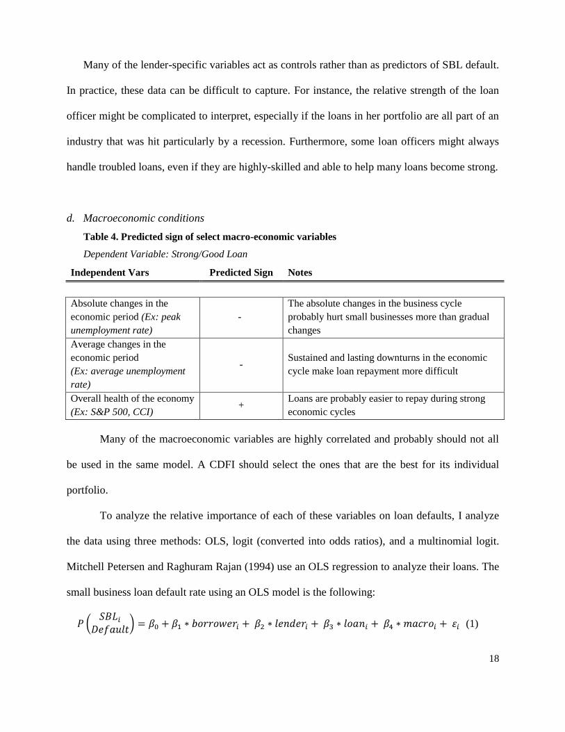
d. Macroeconomic conditions

Table 4. Predicted sign of select macro-economic variables

Dependent Variable: Strong/Good Loan

Independent Vars Predicted Sign Notes

Absolute changes in the

economic period (Ex: peak

unemployment rate)

-

The absolute changes in the business cycle

probably hurt small businesses more than gradual

changes

Average changes in the

economic period

(Ex: average unemployment

rate)

- Sustained and lasting downturns in the economic

cycle make loan repayment more difficult

Overall health of the economy

(Ex: S&P 500, CCI) +

Loans are probably easier to repay during strong

economic cycles

Many of the macroeconomic variables are highly correlated and probably should not all

be used in the same model. A CDFI should select the ones that are the best for its individual

portfolio.

To analyze the relative importance of each of these variables on loan defaults, I analyze

the data using three methods: OLS, logit (converted into odds ratios), and a multinomial logit.

Mitchell Petersen and Raghuram Rajan (1994) use an OLS regression to analyze their loans. The

small business loan default rate using an OLS model is the following:

(1)

19

Where β0 is the constant, ε is the error term, and loan, lender, borrower, and macroeconomic

variables are all specific to the individual loan i. The benefit of an OLS regression is that the

coefficients can be directly interpreted as the relative weights that influence loan defaults. The

downside is that if the SBL default rate is binary, where good loans are equal to 1 and bad loans

are equal to 0, OLS regressions can output values that are greater than 1 or less than 0, which are

nonsensical probabilities.

A logit model solves this problem, because it will not predict probabilities that are greater

than 1 or less than 0. The downside of a logit model is that the coefficients cannot be directly

interpreted (unless converted into an odds ratio), which makes subsequent credit-scoring values

more difficult to calculate. A logit model measures the probably of defaults as the following:

. (2)

Here, is the SBL default rate, contains borrower-specific variables, contains loan-

specific variables, contains lender-specific variables, and contains macroeconomic

variables. The error is assumed to be distributed as a standard logistic. The borrower would

default if and she would repay the loan if . We can

determine the default probability:

)

)

) (3)

Where F is the cumulative density function for ε. For the logit model, this is specified as

20

(4)

The probabilities from a logit model are between 0 and 1:

(5)

(6)

This is a binary logit (“default” or “repaid”). If the dataset differentiates beyond two

dependent variables, such as X’s dataset, where there are three loan repayment options: strong,

medium, or weak loans, a multinomial logit regression can be the best model. The multinomial

logit regression for the model is:

(7)

Where if the loan is strong, M if medium, W if weak, contains borrower-specific

variables, contains loan-specific variables, contains lender-specific variables, and

contains macroeconomic variables. The benefit of a multinomial regression is that a strong loan’s

influences are separately identified from a medium loan and from a weak loan. The drawback is

that calculating a credit score using the multinomial logit method is also more difficult.

IV. Data

The methodology and data in this paper have been IRB approved. The data come from X

CDFI’s original loan files. All of the files are hard copies, and it took numerous people to

compile the dataset. It can take twenty to forty-five minutes to identify and tally all of the

required information for a loan file (Overstreet and Rubin 1996). The dataset contains 530 loans,

which includes 229 SBA loans and 301 non-SBA loans. The S&P 500 information comes from

Datastream, and the S&P values are linked to each loan depending on the date of origination.

The local state-level unemployment rate data is from the Bureau of Labor Statistics.

21

Table 5. Origination dates by loan program

SBA Loans

Non-SBA Loans

Combined Loans

Origination Year Freq. Percent Cum. Freq. Percent Cum. Freq. Percent Cum.

2002 3 1.31 1.31

96 31.89 31.89

99 18.68 18.68

2003 32 13.97 15.28

103 34.22 66.11

135 25.47 44.15

2004 33 14.41 29.69

102 33.89 100

135 25.47 69.62

2005 34 14.85 44.54

34 6.42 76.04

2006 61 26.64 71.18

61 11.51 87.55

2007 66 28.82 100

66 12.45 100

Totals 229 100 301 100 530 100

The non-SBA loans only originate between 2002 and 2004 in this dataset. Although X

CDFI did underwrite non-SBA loans after 2004, the data is not yet in digital form. The

unbalanced combined loan data will have controls to minimize the bias of the earlier origination

dates of the non-SBA loans.

The definition measure of loan default is described in the following table:

Strong Medium Weak

Never delinquent Ever 30+ days delinquent more than once Ever 90+ days delinquent

Never modified Ever 60+ days delinquent Charged off

Ever modified

Notes:

30+, 60+, 90+: If 90+, is not counted as 30+ or 60+

Loans modified for one month (these are mostly non-payment related) or

delinquent one time for 30 days classified as “strong”

The loans in this dataset have a relatively high default rate. Around 26% of all of the

loans are classified as “weak,” 34% are classified as “medium,” and only 39% are classified as

strong. This data comes from a non-random sample, which over emphasizes weak loans. This is

discussed in further detail at the end of this section. Table 6 outlines the frequencies and

cumulative percentage of the loans.

22

Table 6. Loan strength by loan program (as of October 2009)

SBA Loans

non-SBA Loans

Combined Data

Loan Strength Freq. Percent Freq. Percent Freq. Percent

Weak

66 28.82

73 24.25

139 26.23

Medium

67 29.26

116 38.54

183 34.53

Strong

96 41.92

112 37.21

208 39.25

Totals 229 100 301 100 530 100

The data come only from X CDFI and the results of loan default in this sample may not

be indicative of the more general small business market. The following table outlines the

borrower, loan, lender and macroeconomic variables from this dataset.

Table 7. Description of Independent Variables

Indep Var Code Units Notes

Borr

ow

er-S

pec

ific

Management

Experience EXPMAN Continuous

Number of years with management

experience

Female

Borrower FEMALE

Dummy: Female

1, Male 0

Personal FICO

Score FICO_10 Continuous Three digit FICO score divided by 10 pts

Industry Code IND_AGG Categorical Derived from NAISCs codes

Length of

Business LENGTHBUS Continuous Length of business in years

Minority

Borrower MINORITY

Dummy: Minority

1, White 0

The minority variable combines African

American, Asian, Hispanic and "Other"

Debt to Income DI Continuous

The borrower’s debt-to-income before the

loan

Start-up

Business STARTUP

Dummy: Start Up

1, Existing

Business 0

Calculated using Length of Business. Start-

up defined as length business ≤ 1 year

Loa

n a

nd

Len

der

Sp

ecif

ic

Loan Age AGE(M) Continuous

The number of months between the

origination date and the maturity date. If

the loan is still active as of Oct 2009,

10/31/09 is used as the end date.

Guarantee

Percentage GUAR_10 0, 5.0, 7.5, 8.5

SBA 0, and three options for SBA: 50, 75,

and 85% (the interest rate percentage is

divided by 10 units)

23

Interest Rate

Deviation from

Prime

IntDevFromPr Continuous Calculated by subtracting interest rate

10

from the Federal Prime rate

Log of the loan

amount LN(LAMT) Continuous

Matured Loan MATURED

Dummy: Matured

1, Active 0

SBA Loan SBA

Dummy: SBA 1,

non-SBA 0

Variable

Interest Rate VARINT

Dummy: Variable

Rate 1, Fixed 0

Macr

oec

on

om

ic

S&P 500 S&P_Orig Continuous

The market value of the S&P 500 on day

of origination

Peak Change in

Local

Unemployment

UR_DevOrig Continuous

Difference between unemployment at the

origination day and the peak local

unemployment rate over the life of the loan

Inte

ract

ion

Int. Deviation

from Prime x

S&P 500

INTDEVx

SP500 Continuous

Interaction term between the interest rate

and S&P 500 at origination

Variable Rate x

S&P 500

VARINTx

SP500 Continuous

Interaction term between variable interest

rate and S&P 500 at origination

Before going into the empirical specification, some parts of dataset require additional

attention. The literature states that in general, the borrower’s FICO score is one of the most

predictive measures of loan repayment. In the following graph, the values of “strong,”

“medium,” and “weak” were assigned as of October 2009.

10 The interest data are available as follows: if the loan matured, the interest rate is that at maturity. If the loan is active, the

interest rate is that at 10/31/2009. If the loan is fixed (the rate does not change over the course of the loan), the deviation from

prime calculates the deviation between the fixed rate and the Fed Prime rate at origination. If the rate is variable, it calculates

the variable rate at maturity (or at 10/31/2009 if active) and the Federal Reserve Prime rate at maturity (or at 10/31/2009). This

is an important distinction, because most variable interest rates are calculated by X CDFI as the prime rate plus the spread.

Thus for variable rates, the interest rate deviation from prime is the spread. The interpretation of this variable is the relative

interest rate cost for this borrower compared to other rates he or she could find on the market.

24

Figure 2. Better FICO scores are mildly

predictive of loan repayment as of October 2009

As shown in Figure 2, if the CDFI wanted to create a cut-off of 650 for loan applicants,

this would capture both a high number of strong and weak loans. This box plot suggests that

many other factors influence default, and even the historically most predictive factor, FICO

score, does not alone adequately explain a significant portion of the loan strength.

CDFIs have access to two financial sources that are often not available to traditional

banks: grants and subsidies. Grants are a source of revenue that the bank does not have to repay.

Subsidies, in this paper, are defined as loans with subsidized interest rates – interest rates below

market rates. Although these subsidized loans will have to be repaid, they are cheaper than the

ones a bank would find on the market. X has access to investor grants, government guarantees,

or other borrowing methods with interest rates below the market rate. X, however, does not

always entirely pass along these below market interest rates to its borrowers, because it needs use

some of the revenue to finance its internal underwriting costs.11

11 This may bring up the question of X’s profitability, but profitability is out of scope for this research paper.

400 500 600 700 800FICO

Weak Medium Strong

25

Figure 3. Borrowers with better FICO scores pay lower interest rates

On average, borrowers with higher (better) FICO scores pay lower (cheaper) interest

rates on their loans (correlation, ρ= -0.042). The scatter plot also shows some clumping,

particularly around 10% and above 8%. These clusters are due to X’s obliged interest rates for

their program-based (investor-backed) loans. As discussed in the theoretical section, when

interest rates are program-based, they can make good borrowers seem bad and vice versa. The

dataset lacks program identifiers, and I will only be able to control for the known interest rates.

Another way to look at the origination interest rate is to see how much it deviates from the

Federal Prime rate.

Figure 4. Some CDFI borrowers pay below Fed Prime interest rates

46

810

12

14

400 500 600 700 800FICO

Interest Rate Fitted values

0.1

.2.3

De

nsi

ty

-2 0 2 4 6 8Interest Rate Devation from Federal Prime Rate

26

Figure 5. The interest rate deviation from the Fed Prime

rate holds relatively constant across FICO scores

In Figure 4, a value of 0 on the x-axis indicates that the interest rate on the loan and the

Federal Prime rate are the same. Some of the borrowers in this dataset actually pay interest rates

that are cheaper than the Fed rate (Figure 5, ρ=0.014). This is possible because CDFIs are able to

pass along selectively some of their subsidized rates to some of their borrowers. The most

significant limitation with the interest rate data are that some of the variable rates are not

calculated using Fed Prime + Spread. A few of the variables rates also do not update monthly

(see footnote 10 for how the deviation rate is calculated and its assumptions). In addition, the

monthly payments for some borrower do not change with the variable rate, and they only pay

more at the end of the loan’s life. If this occurs, they may not be affected by the changing Fed

Rate. Future iterations of this model would have to include more complete interest rate data.

The small business loan industries are aggregated using NAICS codes. These variables

can be used as controls to minimize the bias of one industry performing better in a period than

another. The frequency and descriptive chart of the industry classifications is below.

-50

510

400 500 600 700 800FICO

Interest Rate Deviation from Prime Rate Fitted values

27

Table 8. Most of the loans are given to retail, recreation, or educational services

Ind.

Code

NAICS

Codes General Name Freq. Percent % Weak

0

No code available 2 0.38 0.00

1 11 Farming 8 1.51 37.50

2 21, 22, 23 Mining, Utilities, Construction 30 5.66 30.00

3 31, 32, 33 Manufacturing 30 5.66 33.33

4 42, 44, 45,

48, 49

Wholesale, Retail Trade, Transportation

and Warehousing 118 22.26 33.05

5 51, 52, 53,

54, 55, 56

Professional, Scientific, Technical

Services, Real Estate, Finance, Insurance,

Waste Management and Remediation

Services

87 16.42 26.44

6 61, 62, 9

Educational Services, Health Care and

Social Assistance, and Public

Administration

105 19.81 13.33

7 71, 72 Arts, Entertainment, Recreation,

Accommodation and Food Services 97 18.30 31.96

8 81 Automotive Repair, Machine and

Equipment Repair, and Personal Care 53 10.00 18.87

Total 530 100

SBLs can be particularly difficult to obtain from a traditional bank, especially if the

company is a start-up. A start-up is defined a firm in business for one year or less.

Figure 6. Most of the loans are for young businesses and start-ups

0.1

.2.3

.4

De

nsity

0 10 20 30 40Length of Business (years)

28

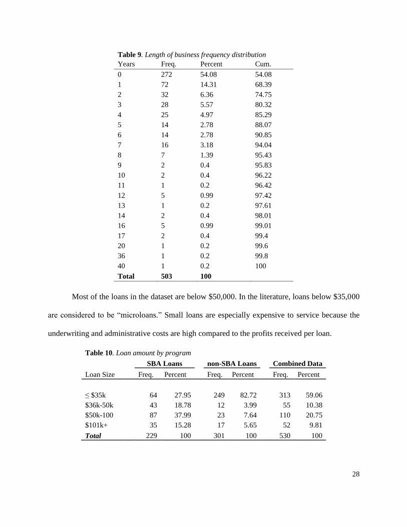
Table 9. Length of business frequency distribution

Years Freq. Percent Cum.

0 272 54.08 54.08

1 72 14.31 68.39

2 32 6.36 74.75

3 28 5.57 80.32

4 25 4.97 85.29

5 14 2.78 88.07

6 14 2.78 90.85

7 16 3.18 94.04

8 7 1.39 95.43

9 2 0.4 95.83

10 2 0.4 96.22

11 1 0.2 96.42

12 5 0.99 97.42

13 1 0.2 97.61

14 2 0.4 98.01

16 5 0.99 99.01

17 2 0.4 99.4

20 1 0.2 99.6

36 1 0.2 99.8

40 1 0.2 100

Total 503 100

Most of the loans in the dataset are below $50,000. In the literature, loans below $35,000

are considered to be “microloans.” Small loans are especially expensive to service because the

underwriting and administrative costs are high compared to the profits received per loan.

Table 10. Loan amount by program

SBA Loans

non-SBA Loans

Combined Data

Loan Size Freq. Percent Freq. Percent Freq. Percent

≤ $35k

64 27.95

249 82.72

313 59.06

$36k-50k

43 18.78

12 3.99

55 10.38

$50k-100

87 37.99

23 7.64

110 20.75

$101k+

35 15.28

17 5.65

52 9.81

Total 229 100 301 100 530 100

29

As noted earlier, CDFIs make an effort to extend loans to women, minorities, and low-

wealth individuals. Of the 530 loans, 479 contain information about the race of the borrower.

Due to the lack of observations, African American, Hispanic, Asian, and other are combined into

a “minority” dummy variable.

Table 11. Race frequency distribution by program

SBA Loans

non-SBA Loans

Combined Data

Race Freq. Percent Freq. Percent Freq. Percent

African American 55 24.77

91 35.41

146 30.48

Hispanic

7 3.15

27 10.51

34 7.1

Asian

3 1.35

4 1.56

7 1.46

White

153 68.92

128 49.81

281 58.66

Other

4 1.8

7 2.72

11 2.3

Total 222 100 257 100 479 100

The number of government-guaranteed SBA loans given to women is almost exactly

equal to men. The non-SBA loans are more commonly given to men, but it also rounds to

approximately half.

Table 12. Female frequency distribution by loan program

SBA Loans

non-SBA Loans

Combined Data

Gender Freq. Percent Freq. Percent Freq. Percent

Male

115 50.22

162 53.82

277 52.26

Female

114 49.78

139 46.18

253 47.47

Total 229 100 301 100 530 100

The data in this paper were collected though a non-random sample. This dataset includes

all of the weak loans in the CDFI’s portfolio and may not include all of the strong loans. I do not

know what percentage of weak/strong loans this sample contains compared to the population at

large, so I cannot reweight my results to control for the non-random sample selection. I had to

assume that this is relatively close to the actual population, and in the future, X would want to re-

run these models when they have the time to collect all of the loan file data digitally.

30

Another weakness in the dataset is that the collection period is limited. The sample does

not contain data on loans before 2002 or after 2007. This means the models not capture loan

performance before the technology bubble in 2001 or during the current crisis, which started in

2008. The data also do not contain any information regarding the borrower’s ability to obtain any

other loans, both from CDFIs or traditional loans. In addition, the dataset lacks information on

the corporate structure of the business (e.g., corporation, partnerships or sole proprietorships).

The dataset in this paper is only from the portfolio from X. Neither I nor X have been

able to access loan-level data from any other CDFI, and, thus, the results from this paper cannot

be compared with CDFIs across the country. The data also do not include any “shocks” to the

borrower or business. Divorce, death in the family, or another major change in the life of a small

business owner could affect his or her ability to repay the loan. The data also do not include

loans that were denied – and X does not keep track of those loans in their digital database. This

means this paper is unable to quantify any “gains” they could have made using the proposed

credit-scoring model.

Furthermore, the data do not differentiate between new loans and renewals. Having a

high level of renewals can be a serious problem in the dataset – especially if the renewal is

paying off the original loan. After discussing this matter with X, they said that they only give

around five renewal loans or fewer each year. They also said it would be difficult to identify the

renewal loans in the dataset because their all of the information is contained in hard-copy files.

Considering its rarity and the difficulty to isolate these renewal loans, I have not made any

corrections for this in my data.

Co-borrowers also could be a problem in the data. Unfortunately, X only tracks one name

per loan and the dataset does not have information on co-borrowers. This information exists also

31

in the hard-copy files, which would again involve a manual tabulation. If there is a co-borrower

it is often the owner and the business that have their names on the loan. In addition, I do not have

any geographically identifying information, such as zip codes, for the loans, which could

improve the results.

The biggest flaw in this dataset is the creation of the dependent variable. The strong,

medium, weak designations are absorptive states. All loans start out as strong and once a loan

becomes medium, it can never go back to strong. Because the data are not time dependent, I do

not know at what time a loan started to be in arrears. This is an important distinction, because a

loan that defaults in month 1 is much worse than a loan that defaults in the last month. A bank

would prefer to recoup 99% of a loan than only 5%. However, in this dataset, both of those loans

would be classified as weak.

Because I do not know when a loan starts to go bad, I cannot state with certainty that any

of the macroeconomic variables affected its late payments. For example, I know the origination

dates and the expected date of maturity for each loan. The average and peak unemployment

variables are calculated using this estimated life of the loan (or if the loan had not matured by

October 2009, 10/31/09 is selected as the “end date”). For instance, if loan Z originated in Feb

2002 and had a maturity date of Dec 2008 and the peak unemployment was 8.1% in late 2008,

but the loan started to become delinquent in 2007, the relationship between the peak local

unemployment and the loan strength would be deceiving. One solution to this would be to

develop a hazard model approach and a corresponding dataset measures the influence of time on

borrower default.

32

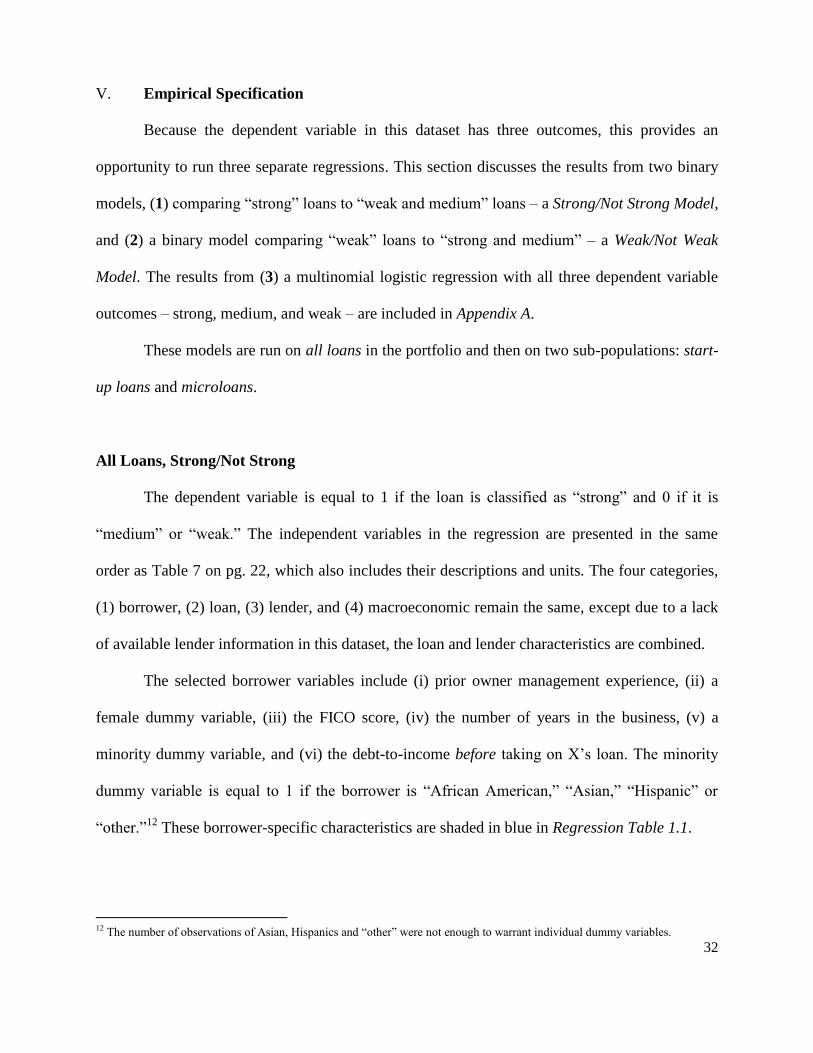
V. Empirical Specification

Because the dependent variable in this dataset has three outcomes, this provides an

opportunity to run three separate regressions. This section discusses the results from two binary

models, (1) comparing “strong” loans to “weak and medium” loans – a Strong/Not Strong Model,

and (2) a binary model comparing “weak” loans to “strong and medium” – a Weak/Not Weak

Model. The results from (3) a multinomial logistic regression with all three dependent variable

outcomes – strong, medium, and weak – are included in Appendix A.

These models are run on all loans in the portfolio and then on two sub-populations: start-

up loans and microloans.

All Loans, Strong/Not Strong

The dependent variable is equal to 1 if the loan is classified as “strong” and 0 if it is

“medium” or “weak.” The independent variables in the regression are presented in the same

order as Table 7 on pg. 22, which also includes their descriptions and units. The four categories,

(1) borrower, (2) loan, (3) lender, and (4) macroeconomic remain the same, except due to a lack

of available lender information in this dataset, the loan and lender characteristics are combined.

The selected borrower variables include (i) prior owner management experience, (ii) a

female dummy variable, (iii) the FICO score, (iv) the number of years in the business, (v) a

minority dummy variable, and (vi) the debt-to-income before taking on X’s loan. The minority

dummy variable is equal to 1 if the borrower is “African American,” “Asian,” “Hispanic” or

“other.”12

These borrower-specific characteristics are shaded in blue in Regression Table 1.1.

12 The number of observations of Asian, Hispanics and “other” were not enough to warrant individual dummy variables.

33

The selected loan and lender variables include: (i) the age of the loan in months, (ii) the

government guarantee percentage of each individual loan, (iii) the deviation of each loan’s

interest rate from the Fed Prime rate, (iv) the natural log of the loan amount, (v) a dummy

variable for whether or not the loan has matured, and (vi) a dummy for whether the loan’s

interest rate is variable or fixed.

The two macroeconomic variables are (i) the market value of the S&P 500 on the day of

origination, and (ii) the peak change in the local unemployment rate over the life of the loan. The

first value captures the over-all economic health on the day the loan originates. The second

economic variable is more specific to the loan. The peaks in the cycle are probably more

challenging for SBL solvency than the average value over the life of the loan (which smoothes

out the peaks). In addition, local unemployment rates are less volatile than other economic

indications, such as the S&P 500.

Finally, because the types of loans change with the economic health of the population, the

regression includes interaction terms. The overall economic climate likely affects the bank’s

assigned interest rate and whether or not the borrower gets a variable rate. The interaction terms

are (i) a combination of the interest rate deviation from prime and the S&P 500 value at

origination and (ii) a combination of the variable interest rate dummy and S&P 500 at

origination. In this dataset, more variable rate loans originate when the economy is strong. The

interaction terms help isolate defaults due to loan characteristics, macro-characteristics or when

the macro-variables influence the loan variables and the combined effect of this on a loan.

The Strong/Not Strong model includes five (5) regressions, which are outlined in

Regression Table 1.1 on pg. 36. The first four regressions use OLS, which has coefficients that

are easier to interpret and more straightforward for credit-scoring. The last regression binds the

34

dependent variable values between 1 and 0, and the coefficients are odds ratios from the logit

regression. When regressing Strong/Not Strong on borrower characteristics, only FICO is

significant in model (1). With each 10 point increase in FICO score, the probability of repayment

increased by 1.4%.

After adding loan and macroeconomic controls in regression (2), matured loans are 17%

less likely to be strong. This makes sense given the absorptive nature of the dependent variable.

A loan that becomes weak can never go back to strong. With 95% significance, for each 1%

increase in the peak unemployment rate, the loan has a 4% chance less likely of being strong.

Sharp peaks of the local unemployment rate burden small businesses.

There are two surprising results in this regression (2). First, it indicates that loans with

greater deviations from Fed Prime (more expensive loans) are more likely to be strong. In

addition, variable rate loans are 25% more likely to be strong. The literature would expect the

opposite sign for both of these variables. This occurs because both of these variables are also

highly correlated with the macroeconomic variables at origination. Using interaction terms

isolates these effects. The interaction terms in regression (3) remove the bias in variable interest

rate and interest deviation from prime. They are now both negative values (expected) and not

significant. The interaction term provides a control for the combined effect of a variable interest

rate given in a strong economy.

In addition in regression (3), loans given during strong climates are more likely to be

weak – perhaps indicating that the CDFI has weaker criteria for their borrowers or weaker

borrowers looked stronger during good business cycles. However, if the economy experienced a

large change in unemployment during the life of the loan, the borrower is much more likely to

35

default. For each 1% increase in local unemployment, the probability of being strong decreases

by 4% (90% confidence), which is the same result in regression (2).

Regression (4) includes industry controls. Even though none of the individual industry

dummies are significant, they still control for unexplained factors in the regression. It is

encouraging to find that most of the values remain the same as (3). The one difference is that

S&P 500 at origination is no longer significant. Of note, even regression (4) only has an R2 of

12.6%. This means that even in the most complete regression, very little of the repayment

variation is explained by conventional variables.

One beneficial way to interpret the logit results is to create an odds ratio table, which is

displayed in column (5). The variables that are significant in the logit regression are also the

same level of significance in the displayed odds ratios. The benefit of an odds ratio table is that

the ratios show the relative importance of each variable (much like the OLS coefficients). For

example, for each 10 unit increase in FICO score, the odds ratio of having a strong loan increases

by 6.7%.

This model displays most of the same results as the OLS regression, with a few

exceptions. The odds ratio model indicates loans with large interest rate deviations from the

Federal Reserve rate are more likely to be weak. This makes sense because expensive loans are

likely harder to pay-off. Significant at the 95% level, for each 10 point increase in the S&P 500

at origination, the odds of being a strong loan decreases by 5%. This is weakly significant in

regression (3) and not significant in (4). This echoes the same reasoning as the OLS regression:

either loans given in strong periods have weaker selection criteria or weak borrowers can seem

stronger during these strong economic cycles.

36

Regression 1.1 All Loans [Dependent Variable: Strong=1, Not Strong=0]

(1) OLS (2) OLS (3) OLS (4) OLS (5) Logistic

VARIABLES Borrower-

specific

Includes

macro

Interaction

terms incl.

Industry

controls

Odds

Ratios

Bo

rro

wer

-Spec

ific

Var

iable

s Management Exp. (yrs) 0.002 0.002 0.002 0.001 1.009

(0.003) (0.003) (0.003) (0.003) (0.015)

Female (dummy) -0.010 0.017 0.017 -0.004 1.069

(0.046) (0.047) (0.046) (0.048) (0.232)

FICO 0.014*** 0.013*** 0.013*** 0.014*** 1.061***

(0.004) (0.004) (0.004) (0.004) (0.020)

Length Business (yrs.) 0.008 0.005 0.006 0.006 1.025

(0.006) (0.006) (0.006) (0.006) (0.027)

Minority (dummy) -0.059 -0.041 -0.044 -0.059 0.833

(0.048) (0.048) (0.047) (0.049) (0.187)

Debt-to-income -0.004 -0.002 -0.003 0.000 0.948

(0.014) (0.014) (0.014) (0.014) (0.155)

Loan

and L

ender

Spec

ific

Age of loan (months) -0.002 -0.003 -0.004 0.991

(0.002) (0.002) (0.002) (0.011)

Gov’t Guar. % -0.013 -0.011 -0.010 0.946

(0.009) (0.009) (0.010) (0.043)

Int Deviation from Prime 0.027** -0.132 -0.100 0.402**

(0.013) (0.081) (0.082) (0.183)

Ln(Loan Amount) 0.012 0.023 0.026 1.129

(0.035) (0.035) (0.036) (0.186)

Matured (dummy) -0.169* -0.182* -0.178* 0.408*

(0.096) (0.096) (0.099) (0.205)

Variable Rate (dummy) 0.247*** -0.231 -0.074 0.075

(0.067) (0.373) (0.382) (0.154)

Mac

ro S&P 500 at origination -0.000 -0.007* -0.006 0.949**

(0.002) (0.004) (0.004) (0.021)

Peak ∆ Local Unemp. Rate -0.040** -0.040* -0.037* 0.798**

(0.020) (0.021) (0.021) (0.085)

Interest Dev*S&P 500 0.001* 0.001* 1.009**

(0.001) (0.001) (0.004)

Variable Rate*S&P 500 0.004 0.002 1.033*

(0.003) (0.003) (0.019)

Constant -0.518** -0.434 0.270 0.168

(0.252) (0.498) (0.590) (0.688)

Industry Controls? No No No Yes No

Observations 443 443 443 443 443

R-squared 0.045 0.099 0.110 0.126 LR χ2(16)=54.1

Adj. R-squared 0.032 0.069 0.076 0.076 Prob>χ2 = 0.00

Standard errors in parentheses

*** p<0.01, ** p<0.05, * p<0.1

37

All Loans, Weak/Not Weak

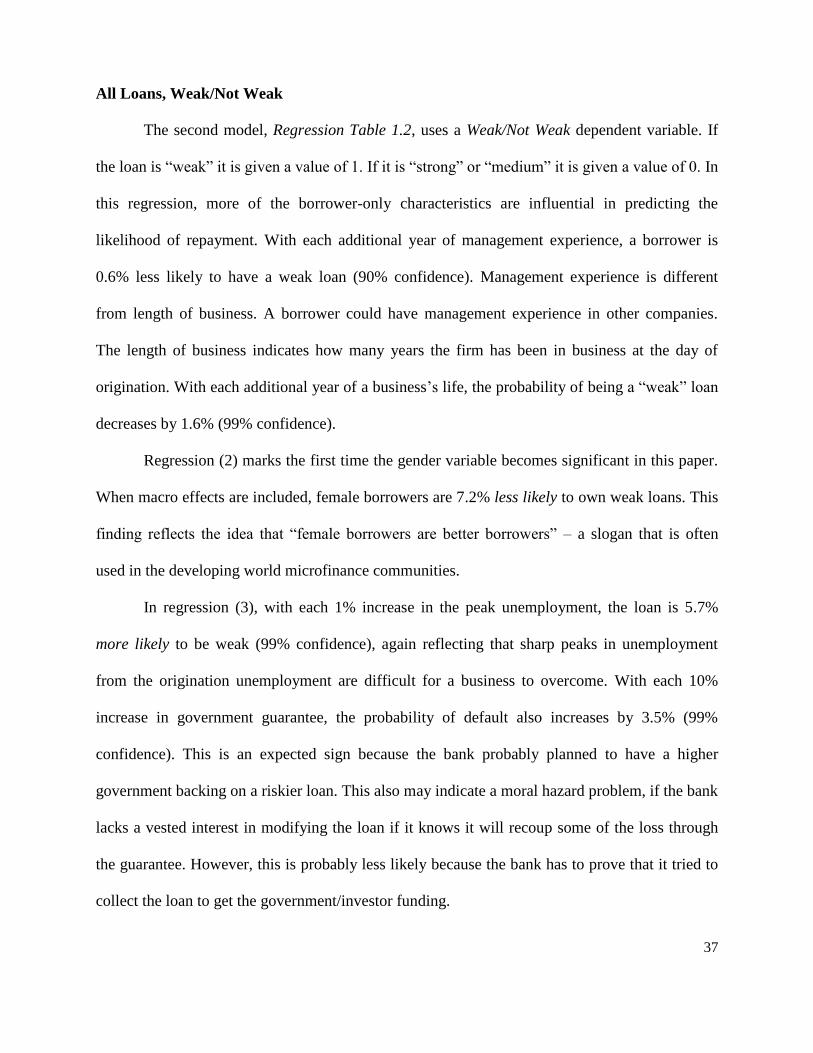
The second model, Regression Table 1.2, uses a Weak/Not Weak dependent variable. If

the loan is “weak” it is given a value of 1. If it is “strong” or “medium” it is given a value of 0. In

this regression, more of the borrower-only characteristics are influential in predicting the

likelihood of repayment. With each additional year of management experience, a borrower is

0.6% less likely to have a weak loan (90% confidence). Management experience is different

from length of business. A borrower could have management experience in other companies.

The length of business indicates how many years the firm has been in business at the day of

origination. With each additional year of a business’s life, the probability of being a “weak” loan

decreases by 1.6% (99% confidence).

Regression (2) marks the first time the gender variable becomes significant in this paper.

When macro effects are included, female borrowers are 7.2% less likely to own weak loans. This

finding reflects the idea that “female borrowers are better borrowers” – a slogan that is often

used in the developing world microfinance communities.

In regression (3), with each 1% increase in the peak unemployment, the loan is 5.7%

more likely to be weak (99% confidence), again reflecting that sharp peaks in unemployment

from the origination unemployment are difficult for a business to overcome. With each 10%

increase in government guarantee, the probability of default also increases by 3.5% (99%

confidence). This is an expected sign because the bank probably planned to have a higher

government backing on a riskier loan. This also may indicate a moral hazard problem, if the bank

lacks a vested interest in modifying the loan if it knows it will recoup some of the loss through

the guarantee. However, this is probably less likely because the bank has to prove that it tried to

collect the loan to get the government/investor funding.

38

In addition, with each 1% increase in the interest rate deviation from prime (e.g. a more

expensive loan), the loan is 16% more likely to be weak. Although the sign is expected, this is a

surprisingly large effect and likely depends on the investor-assigned program-based interest

rates. However, given the ambiguity of the variable-rate data, this may not be the true size. The

counterintuitive negative sign on the variable interest rate dummy in (2) has now become

somewhat more conventional in (3), because interaction terms remove the bias of variable rates

given in strong economic climates. Regression (3) states that a variable interest rate loan is 59%

more likely to be weak (90% confidence). Although the sign is expected, the magnitude is large.

Although none of the industry dummies are individually significant, when industry

controls are included (4), most of the results stay the same with one exception: the variable rate

is no longer significant. The R2 in (4) of the Weak/Not Weak regression is 27%, and is much

better than in the Strong/Not Strong (4), which is 7.6%, but these conventional variables still

explain little of the overall variation. This is because default often occurs due to unobserved

characteristics, such as a crisis in the personal life of the small business owner or shocks in the

cost structure of the small business.

The final column (5) displays the odds ratios. With each year increase in the business, the

loan has 13% lower odds of being weak. With each 10 point increase in FICO, the odds of being

weak also decrease by 9%. Each 10% increase in government guarantee increases the odds of a

weak loan by 34%. This could again reflect that the bank is willing to take on a riskier borrower

only if there is some government guarantee. The odds ratio results are comparable to the OLS

regression, except that in the odds ratios, it indicates with more significance that women are less

likely to hold weak loans than men – women have a 46% lower odds of holding a weak loan.

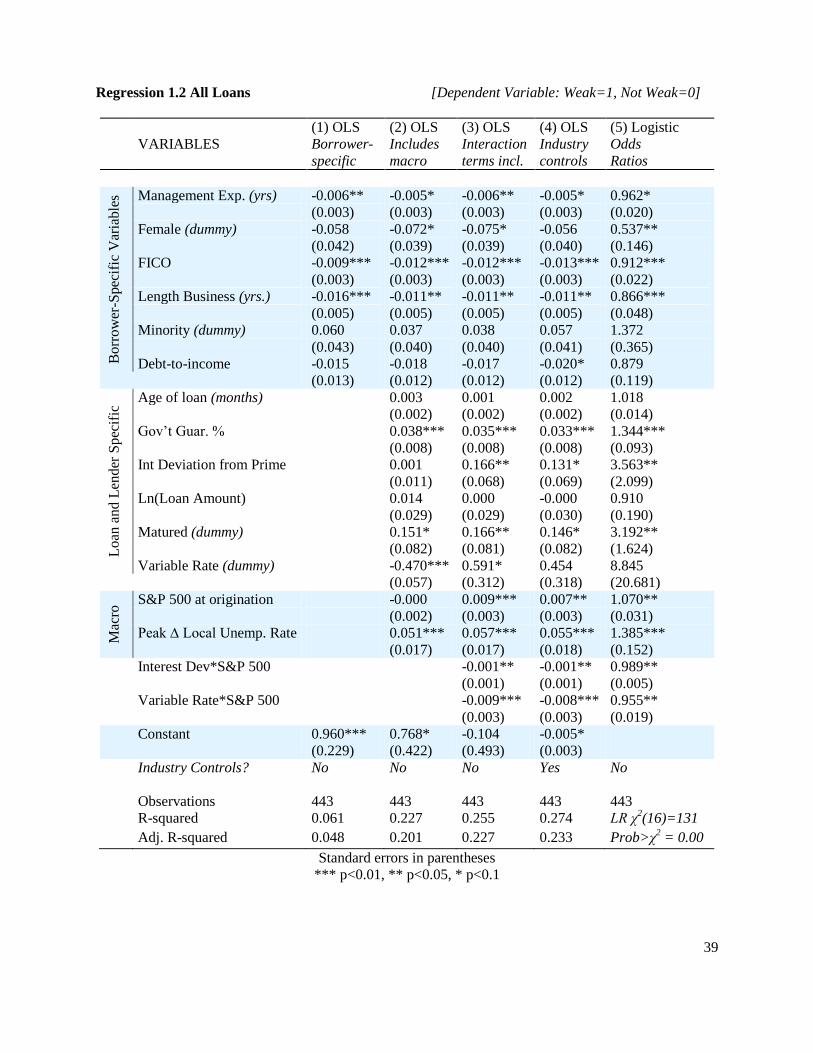
The multinomial logistic regression for all loans is discussed in Appendix A.

39

Regression 1.2 All Loans [Dependent Variable: Weak=1, Not Weak=0]

(1) OLS (2) OLS (3) OLS (4) OLS (5) Logistic

VARIABLES Borrower-

specific

Includes

macro

Interaction

terms incl.

Industry

controls

Odds

Ratios

Bo

rro

wer

-Spec

ific

Var

iable

s Management Exp. (yrs) -0.006** -0.005* -0.006** -0.005* 0.962*

(0.003) (0.003) (0.003) (0.003) (0.020)

Female (dummy) -0.058 -0.072* -0.075* -0.056 0.537**

(0.042) (0.039) (0.039) (0.040) (0.146)

FICO -0.009*** -0.012*** -0.012*** -0.013*** 0.912***

(0.003) (0.003) (0.003) (0.003) (0.022)

Length Business (yrs.) -0.016*** -0.011** -0.011** -0.011** 0.866***

(0.005) (0.005) (0.005) (0.005) (0.048)

Minority (dummy) 0.060 0.037 0.038 0.057 1.372

(0.043) (0.040) (0.040) (0.041) (0.365)

Debt-to-income -0.015 -0.018 -0.017 -0.020* 0.879

(0.013) (0.012) (0.012) (0.012) (0.119)

Loan

and L

ender

Spec

ific

Age of loan (months) 0.003 0.001 0.002 1.018

(0.002) (0.002) (0.002) (0.014)

Gov’t Guar. % 0.038*** 0.035*** 0.033*** 1.344***

(0.008) (0.008) (0.008) (0.093)

Int Deviation from Prime 0.001 0.166** 0.131* 3.563**

(0.011) (0.068) (0.069) (2.099)

Ln(Loan Amount) 0.014 0.000 -0.000 0.910

(0.029) (0.029) (0.030) (0.190)

Matured (dummy) 0.151* 0.166** 0.146* 3.192**

(0.082) (0.081) (0.082) (1.624)

Variable Rate (dummy) -0.470*** 0.591* 0.454 8.845

(0.057) (0.312) (0.318) (20.681)

Mac

ro S&P 500 at origination -0.000 0.009*** 0.007** 1.070**

(0.002) (0.003) (0.003) (0.031)

Peak ∆ Local Unemp. Rate 0.051*** 0.057*** 0.055*** 1.385***

(0.017) (0.017) (0.018) (0.152)

Interest Dev*S&P 500 -0.001** -0.001** 0.989**

(0.001) (0.001) (0.005)

Variable Rate*S&P 500 -0.009*** -0.008*** 0.955**

(0.003) (0.003) (0.019)

Constant 0.960*** 0.768* -0.104 -0.005*

(0.229) (0.422) (0.493) (0.003)

Industry Controls? No No No Yes No

Observations 443 443 443 443 443

R-squared 0.061 0.227 0.255 0.274 LR χ2(16)=131

Adj. R-squared 0.048 0.201 0.227 0.233 Prob>χ2 = 0.00

Standard errors in parentheses

*** p<0.01, ** p<0.05, * p<0.1

40

Start-Up Loans, Strong/Not Strong

The CDFI data has two important sub-groups that should be looked at separately: (1)

start-up loans and (2) microloans. Start-up loans are businesses that have been in business for a

year or less. The Strong/Not Strong start-up loan regressions are displayed in Regression 2.1.

The five regressions on the start-up loans are similar to the outputs on the all-loans model. This

section highlights the differences.

In general, high FICO scores have more of an impact on loan strength in start-up loans

than in the all-loans model. Comparing (4), in start-up loans a 10 point increase in FICO

increases the probability of a strong loan by 1.7% compared to 1.4% in the all-loans regression.

Although the interest rate deviation from prime is significant in the all-loans model, it is not

significant in the start-up loan model. This could mean that start-up borrowers are not as

sensitive to interest rates as borrowers on the whole. Although this may sound surprising,

perhaps it is because the entire population includes micro-borrowers and other types of

borrowers, who could be much more sensitive to interest rate deviations.

In the logistic regression, variable-rate loans are significantly more likely to be weak for

start-up loans. The all-loans analysis does not find this result. This suggests that start-up

borrowers have more difficulty paying off variable interest rates than other borrowers. Finally,

start-up borrowers are more sensitive to peak changes in the local unemployment rate.

Comparing (4), for each 1% change in the peak rate, start-up borrowers are 4.8% more likely to

default, compared to 3.7% for all loans.

41

Regression 2.1 Start-up Loans [Dependent Variable: Strong=1, Not Strong=0]

(1) OLS (2) OLS (3) OLS (4) OLS (5) Logistic

VARIABLES Borrower-

specific

Includes

macro

Interaction

terms incl.

Industry

Controls

Odds

Ratios

Management Exp. (yrs) 0.001 -0.000 0.000 0.001 1.004

(0.004) (0.004) (0.004) (0.004) (0.019)

Female (dummy) -0.008 0.027 0.030 0.001 1.146

(0.055) (0.056) (0.056) (0.056) (0.310)

FICO 0.014*** 0.016*** 0.016*** 0.017*** 1.079***

(0.004) (0.005) (0.005) (0.005) (0.025)

Length Business (yrs.) -0.047 -0.039 -0.036 -0.017 0.813

(0.068) (0.069) (0.069) (0.070) (0.281)

Minority (dummy) -0.077 -0.064 -0.065 -0.068 0.741

(0.057) (0.057) (0.057) (0.057) (0.210)

Debt-to-income -0.003 -0.002 -0.002 0.001 0.921

(0.014) (0.014) (0.014) (0.014) (0.238)

Age of loan (months) -0.002 -0.001 -0.003 0.999

(0.002) (0.003) (0.003) (0.014)

Gov’t Guar. % -0.018 -0.013 -0.011 0.930

(0.012) (0.012) (0.012) (0.056)

Int Deviation from Prime 0.014 -0.105 -0.055 0.399

(0.016) (0.094) (0.095) (0.229)

Ln(Loan Amount) 0.007 0.014 0.016 1.066

(0.043) (0.043) (0.045) (0.226)

Matured (dummy) -0.223** -0.220** -0.226** 0.308*

(0.111) (0.111) (0.113) (0.193)

Variable Rate (dummy) 0.301*** -0.392 -0.220 0.013*

(0.078) (0.434) (0.437) (0.035)

S&P 500 at origination -0.002 -0.008* -0.007 0.937**

(0.003) (0.004) (0.004) (0.027)

Peak ∆ Local Unemp. Rate -0.048** -0.051** -0.048** 0.719**

(0.023) (0.023) (0.024) (0.097)

Interest Dev*S&P 500 0.001 0.001 1.009*

(0.001) (0.001) (0.005)

Variable Rate*S&P 500 0.006 0.004 1.053**

(0.004) (0.004) (0.025)

Constant -0.566* -0.322 0.319 0.319

(0.306) (0.598) (0.709) (0.709)

Industry Controls? No No No Yes No

Observations 309 309 309 309 309

R-squared 0.053 0.123 0.134 0.134 LR χ2(16)=48.4

Adj. R-squared 0.034 0.081 0.086 0.086 Prob>χ2 = 0.00

Standard errors in parentheses

*** p<0.01, ** p<0.05, * p<0.1

42

Start-Up Loans, Weak/Not Weak

In the Weak/Not Weak model in Regression 2.2 for start-up loans had similar results as

the all loans regression. The following section highlights the differences.

Management experience is significant in predicting default for all-loans, but it is not

significant for predicting default in start-up loans. Although the start-up borrowers in general

have less experience than the all-loan borrowers in the data, this does not explain entirely why it

is not significant. It is a surprising result, because the literature suggests that start-ups fare better

if the founder has more work experience.

Additionally, the length of the business (in years) is highly significant for all-loans, and

intuitively, the length of business is not significant for the start-up loans – because by definition,

start-up loans are those in business for a year or less. The rest of the numbers in start-up model

are comparable to the all loans model.

The relative risk ratio for the multinomial logistic regression for start-up loans is

discussed in Appendix A.

43

Regression 2.2 Start-Up Loans [Dependent Variable: Weak=1, Not Weak=0]

(1) OLS (2) OLS (3) OLS (4) OLS (5) Logistic

VARIABLES Borrower-

specific

Includes

macro

Interaction

terms incl.

Industry

Controls

Odds

Ratios

Management Exp. (yrs) -0.006 -0.003 -0.004 -0.003 0.972

(0.004) (0.004) (0.004) (0.004) (0.022)

Female (dummy) -0.065 -0.090* -0.094* -0.074 0.540**

(0.053) (0.050) (0.050) (0.051) (0.167)

FICO -0.011** -0.016*** -0.015*** -0.016*** 0.913***

(0.004) (0.004) (0.004) (0.004) (0.024)

Length Business (yrs.) 0.026 0.028 0.024 0.005 1.075

(0.065) (0.062) (0.062) (0.064) (0.385)

Minority (dummy) 0.061 0.045 0.045 0.051 1.296

(0.055) (0.051) (0.051) (0.052) (0.394)

Debt-to-income -0.016 -0.017 -0.016 -0.019 0.889

(0.014) (0.013) (0.013) (0.013) (0.126)

Age of loan (months) 0.001 0.000 -0.000 1.006

(0.002) (0.002) (0.003) (0.016)

Gov’t Guar. % 0.041*** 0.035*** 0.031*** 1.292***

(0.011) (0.011) (0.011) (0.105)

Int Deviation from Prime 0.003 0.121 0.085 2.847*

(0.015) (0.085) (0.086) (1.774)

Ln(Loan Amount) 0.036 0.030 0.040 1.124

(0.039) (0.039) (0.040) (0.279)

Matured (dummy) 0.198** 0.191* 0.174* 3.278**

(0.101) (0.100) (0.102) (1.924)

Variable Rate (dummy) -0.520*** 0.415 0.334 5.638

(0.071) (0.390) (0.395) (14.544)

S&P 500 at origination 0.002 0.009** 0.007* 1.066**

(0.002) (0.004) (0.004) (0.033)

Peak ∆ Local Unemp. Rate 0.051** 0.057*** 0.056*** 1.355**

(0.021) (0.021) (0.021) (0.169)

Interest Dev*S&P 500 -0.001 -0.001 0.992

(0.001) (0.001) (0.006)

Variable Rate*S&P 500 -0.008** -0.007** 0.960*

(0.003) (0.003) (0.021)

Constant 1.085*** 0.586 -0.117 -0.003

(0.295) (0.541) (0.638) (0.004)

Industry Controls? No No No Yes No

Observations 309 309 309 309 309

R-squared 0.047 0.223 0.242 0.271 LR χ2(16)=83.1

Adj. R-squared 0.028 0.186 0.200 0.209 Prob>χ2 = 0.00

Standard errors in parentheses

*** p<0.01, ** p<0.05, * p<0.1

44

Microloans, Strong/Not Strong

Microloans are loans under $35,000, which is the industry standard cut-off point for

microloans. Microloans are among the most expensive to service because the loan amounts and

corresponding interest rates are often too small to offset the underwriting and servicing costs.

Pre-approval systems or semi-automatic credit-scoring systems for microloans can help reduce

these burdens. The microloan results for Strong/Not Strong are displayed in Regression 3.1. The

regressions for the microloans are also similar to the all loans and start-up loans. The following

section highlights the differences.

Microloan default is less influenced by FICO than start-up or all loans. With every 10

point increase in FICO, the probability of being a strong loan only increases by 1.2% for micro-

borrowers, compared to 1.4% (all-loans) and 1.7% (start-up). This makes sense, because micro-

borrowers are often not well represented (if represented at all) in national credit-scoring

databases. Julie Gerschick (2002) echoes this finding, citing that many micro-borrowers often

borrow from family members and pawnshops which often lack a credit bureau rating or report.

With each 10% increase in government guarantee, the microloans are more likely to be

strong (model 5). This is a surprising result, because the expectation would be less likely to be

strong. This suggests that these “good” micro-borrowers may be untraditional and have trouble

finding funds for good business proposals unless they have government guarantees.

Micro-borrowers are also much more sensitive to deviations in the interest rate. For each

1% increase compared to the Fed Rate, micro-borrowers are 27% less likely to be strong. This

large number, and likely explains why this shows up weakly in the all-loans model (which

includes micro-borrowers) but not in the start-up loans (which does not include micro-

borrowers).

45

Interestingly, loans given to micro-borrowers during strong economic climates are much

more likely to default than loans given to start-up borrowers or borrowers in the all-loans model.

With each 10 point increase in the S&P 500 at origination, micro-borrowers are 1.7% more

likely to default compared to 0.6% (all loans) and 0.7% (start-up loans). This may suggest that

underwriting criteria for micro-borrowers is more lenient in good business cycles, or that micro-

borrowers appear to be stronger during these times.

The loan amount variable is not significant for all loans or start-up loans, but it does

become weakly significant (90% confidence) for micro-borrowers. Micro-borrowers who took

out larger loans are more likely to repay them.

46

Regression 3.1 Microloans (Loans under $35k) [Dependent Variable: Strong=1, Not Strong=0]

(1) OLS (2) OLS (3) OLS (4) OLS (5) Logistic

VARIABLES Borrower-

specific

Includes

macro

Interaction

terms incl.

Industry

Controls

Odds

Ratios

Management Exp. (yrs) 0.000 0.001 0.000 0.000 1.004

(0.005) (0.005) (0.005) (0.005) (0.021)

Female (dummy) -0.028 0.014 -0.000 -0.018 1.024

(0.061) (0.064) (0.064) (0.066) (0.310)

FICO 0.015*** 0.013** 0.012** 0.012** 1.060**

(0.005) (0.005) (0.005) (0.005) (0.026)

Length Business (yrs.) -0.004 -0.003 -0.003 -0.005 0.984

(0.008) (0.008) (0.008) (0.008) (0.038)

Minority (dummy) -0.082 -0.065 -0.075 -0.096 0.628

(0.061) (0.062) (0.061) (0.064) (0.189)

Debt-to-income -0.007 -0.004 -0.007 -0.006 0.497

(0.014) (0.015) (0.015) (0.015) (0.313)

Age of loan (months) -0.001 -0.002 -0.003 0.990

(0.003) (0.003) (0.003) (0.014)

Gov’t Guar. % 0.020 0.070 0.062 1.461*

(0.036) (0.043) (0.043) (0.325)

Int Deviation from Prime 0.015 -0.329** -0.270* 0.162**

(0.022) (0.154) (0.159) (0.129)

Ln(Loan Amount) 0.078 0.078 0.085* 1.526*

(0.050) (0.050) (0.051) (0.378)

Matured (dummy) -0.180 -0.204 -0.210 0.303

(0.169) (0.168) (0.171) (0.296)

Variable Rate (dummy) 0.180 -1.960 -1.646 0.000*

(0.190) (1.238) (1.270) (0.000)

S&P 500 at origination -0.002 -0.018** -0.017** 0.904***

(0.003) (0.007) (0.008) (0.035)

Peak ∆ Local Unemp. Rate -0.057** -0.047 -0.039 0.773

(0.029) (0.029) (0.029) (0.129)

Interest Dev*S&P 500 0.003** 0.003* 1.019**

(0.001) (0.001) (0.008)

Variable Rate*S&P 500 0.014 0.011 1.080*

(0.009) (0.009) (0.048)

Constant -0.532* -0.748 1.039 0.769

(0.322) (0.614) (0.980) (1.027)

Industry Controls? No No No Yes No

Observations 256 256 256 256 256

R-squared 0.054 0.096 0.116 0.136 LR χ2(16)=34.3

Adj. R-squared 0.031 0.043 0.057 0.046 Prob>χ2 = 0.00

Standard errors in parentheses

*** p<0.01, ** p<0.05, * p<0.1

47

Microloans, Weak/Not Weak

In Regression 3.2, the new dependent variable is Weak/Not Weak for microloans. The

results in this section are also similar to the results for Weak/Not Weak in the start-up and all-

loan models. The following section highlights the differences.

The micro-borrower Weak/Not Weak regressions mark the first time debt-to-income

becomes significant. For each 0.01 increase in the debt-to-income ratio for a micro-borrower, the

loan becomes 2.2% more likely to be weak. This variable is not significant in the all-loans and

start-up loans models. This indicates that micro-borrowers who have more debt in their personal

portfolios are more likely to default when taking out business debt (a microloan).

In contrast, the Strong/Not Strong microloan model suggests that borrowers who take on

larger loans are more likely to repay. Combined, these models indicate that borrowers with lots

of personal debt are more likely to default, but borrowers who take out larger debts for their

business are less likely to default. Perhaps, the underlying reason is simply that micro-borrowers

with high levels of pre-loan personal debt have a different type of character from borrowers from

those who take out large microloans. In addition, because many of these micro-borrowers are not

adequately represented in the consumer (FICO) credit bureaus, the borrowers with high levels of

debt should have lower FICO scores. If the FICO scores correctly reflected this, perhaps the

debt-to-income variable would not be significant. More analysis would need to be done to

synthesize what these conflicting results mean.

Interestingly, government guarantees are not significant in predicting microloan default

in model (4), even though these guarantees are significant for all-loans and start-up loans.13

Perhaps the lack of significance on the guarantee variable, like in the Strong/Not Strong micro

13 Of note, only 22% of the microloans have government guarantees.

48

analysis, indicates that micro-borrowers are unable to get loans elsewhere, even though they are

strong borrowers, because they seem “risky.” The higher government guarantees likely

encourage the CDFI to extend credit to (good) borrowers that they might not normally want to

underwrite. Therefore, the lack of significance on this variable could indicate that the guarantees

are going to the “right” type of borrower – someone who is strong, but seems riskier by

conventional measurements.

Management experience for micro-borrowers, like start-up borrowers, is not significant.

In contrast, this is predictive for the all-loans data. Comparing the third models, female micro-

borrowers are much less likely to be weak than men (11% less likely) than start-up females (9.4%

less likely) and all loan females (7.5% less likely to be weak).

The interest variables in the microloan analysis need additional attention. The (4) model,

with industry controls, indicates that with each 1% increase in deviation from Federal Prime,

micro-lenders are 35% more likely to be weak compared to 16% (all loans) and not significant

for start-up loans. In addition, variable-rate loans given to micro-borrowers are 221% more likely

to be weak, compared to 59% (all loans) and not significant for start-up loans. Both of these

numbers for micro-borrowers are extraordinarily large. In part, this could be because only 18%

of microloans have variable rates, and of that 18%, 96% are SBA loans. Of the fixed rate loans,

only 4% are SBA. If the SBA and non-SBA populations are significantly different, which they

likely are, this could explain the large values on variable rate and interest rate deviation for the

micro-borrowers. Perhaps SBA variable-rate loans default in micro-borrower populations at an

exceptionally high rate.

The relative risk ratio for the multinomial logistic regression for microloans is discussed

in Appendix A.

49

Regression 3.2 Microloans (Loans under $35k) [Dependent Variable: Weak=1, Not Weak=0]

(1) OLS (2) OLS (3) OLS (4) OLS (5) Logistic

VARIABLES Borrower-

specific

Includes

macro

Interaction

terms incl.

Industry

Controls

Odds

Ratios

Management Exp. (yrs) -0.005 -0.005 -0.005 -0.005 0.968

(0.004) (0.004) (0.004) (0.004) (0.028)

Female (dummy) -0.085 -0.129** -0.110** -0.107* 0.406**

(0.056) (0.056) (0.055) (0.057) (0.147)

FICO -0.016*** -0.017*** -0.016*** -0.017*** 0.888***

(0.004) (0.005) (0.004) (0.005) (0.028)

Length Business (yrs.) -0.013* -0.015** -0.015** -0.015** 0.851**

(0.007) (0.007) (0.007) (0.007) (0.060)

Minority (dummy) 0.053 0.040 0.051 0.061 1.302

(0.055) (0.054) (0.053) (0.055) (0.443)

Debt-to-income -0.016 -0.025* -0.022* -0.022* 0.867

(0.013) (0.013) (0.013) (0.013) (0.131)

Age of loan (months) 0.005* 0.005** 0.005* 1.042**

(0.003) (0.003) (0.003) (0.019)

Gov’t Guar. % 0.060* 0.008 0.008 1.040

(0.031) (0.037) (0.038) (0.433)

Int Deviation from Prime 0.016 0.396*** 0.351** 123.430***

(0.019) (0.134) (0.138) (209.413)

Ln(Loan Amount) -0.033 -0.032 -0.034 0.889

(0.044) (0.043) (0.044) (0.253)

Matured (dummy) 0.096 0.126 0.129 3.232

(0.149) (0.146) (0.148) (2.658)

Variable Rate (dummy) -0.607*** 2.448** 2.206** 4.608e+13***

(0.166) (1.073) (1.099) (4.914e+14)

S&P 500 at origination 0.001 0.019*** 0.017** 1.269***

(0.003) (0.006) (0.007) (0.107)

Peak ∆ Local Unemp. Rate 0.057** 0.045* 0.042* 1.242

(0.025) (0.025) (0.025) (0.177)

Interest Dev*S&P 500 -0.004*** -0.003*** 0.957***

(0.001) (0.001) (0.015)

Variable Rate*S&P 500 -0.020*** -0.018** 0.777***

(0.008) (0.008) (0.064)

Constant 1.371*** 1.358** -0.683 -0.307

(0.293) (0.539) (0.849) (0.889)

Industry Controls? No No No Yes No

Observations 256 256 256 256 256

R-squared 0.083 0.187 0.223 0.243 LR χ2(16)=71.5

Adj. R-squared 0.061 0.140 0.171 0.164 Prob>χ2 = 0.00

Standard errors in parentheses

*** p<0.01, ** p<0.05, * p<0.1

50

VI. Case-Study Application of Loan Default Model

The analysis in the empirical specification effectively creates the foundation for a CDFI

credit-scoring model. In the OLS regression, the coefficients indicate how much each variable

influences the default rate. Suppose a simple model is the following:

Pdefault = (-0.038)*FICO + (-0.12)*LengthBus + 50.1

For loan Z, if the FICO score is 650 and the length in business is 5 years, then the Pdefault,z

is 24.8. We assign an in-house credit score of 248. In this example of an in-house model, lower

scores are better because they reflect lower probabilities of default. For the Strong/Not Strong

models, higher scores are better. For the Weak/Not Weak models, lower scores are better. Any of

the regression tables could serve as a credit-scoring model, and all of the OLS models are the

simplest to use because the loan officer would just multiply the coefficients by the independent

variable values for the loan in question.

Overstreet and Rubin (1996) recommend that any credit-scoring model should be built on

a set of past applications of at least 1,500 loans. Claire and Kossmann (2003) recommend 15,000

loans, and BankAmerica developed a model based on 15,000 good and 15,000 bad loans

(Oppenheim 1996). X’s dataset only includes 530 loans – a number far below the three

recommendations. Customized score cards cost between $35,000 and $50,000, mainly due to the

number of person-hours needed to sift through loan files (Overstreet et al., 1996). As noted

earlier, it can take 20 to 45 minutes to identify and tally all of the required information for a loan

file; assuming 1,500 loan observations, this could require 1000 person hours.

In addition, Regulation B of the Equal Credit Opportunity Act amendments of 1976

regulates what variables can be included in a credit score. Some of the barred variables include

race, sex, color, religion, and information about marital status, childbearing preferences, and age

51

(Overstreet et al., 1996). Furthermore, if a variable (such as zip code) is highly correlated with

another variable (such as race) and it is also a statistically significant predictor of repayment, it

cannot be used because the chain of causality links it to a variable barred in Regulation B

(Overstreet et al., 1996).

The results from the empirical section in Section V are stronger when tested. An optimal

credit-scoring model uses 2/3 of the data to produce the model, and then tests the model on the

“out-of-sample” data (the remaining 1/3). Given that the dataset already contains fewer than the

optimal amount of loans, the predictive power would be greatly diminished if a model was

created using just 2/3 of the 530 observations. Another way to test the accuracy of the model is

use the odds-ratios. Using the logistic odds ratio probabilities and a threshold of >0.5 probability

equals 1 and <0.5 probability equals 0, the accuracy of the Strong/Not Strong All Loans model is:

Table 13. All Loans Strong/Not Strong Model correctly predicts 85% of the not strong loans

Predicted Values from Model

Predicted Not Strong Predicted Strong

Act

ual

Data

fro

m

Oct

’09 Not Strong 235 41 276

85.14% 14.86 100%

Strong 113 54 167

67.66% 32.34% 100%

Total 348 95 443

78.56% 21.44% 100%

This means that with a 0.5 probability threshold, the Strong/Not Strong All Loans model

correctly predicts a not strong designation 85% of the time and a strong designation 32% of the

time. Considering that the R2 value of the model is only 11%, this is a promising result.

It is difficult to compare these results to other studies, because few, if any, CDFIs have

credit-scoring models, and there is a dearth of academic work on this subject. The internal Kinat

Report at X created a model for SBA-only loans with a predictive power of 76% correct for “not

weak” SBA loans. This model, as shown below, improves the predictive power by correctly

52

predicting 95% of “not weak” loans for SBA and non-SBA loans combined. The Weak/Not

Weak All Loans model predictive power is below:

Table 14. All Loans Weak/Not Weak Model correctly predicts not weak 95% of the time

Predicted Values from Model

Predicted Not Weak Predicted Weak

Act

ual

Da

ta f

rom

Oct

’09 Not Weak 309 15 324

95.37% 4.63% 100%

Weak 68 71 119

57.14% 42.86% 100%

Total 377 66 443

85.10% 14.90% 100%

All of the models are better at predicting the “weak and medium” or the “strong and

medium” combinations. Table 15 shows the correct predictions for each model:

Table 15. Each loan’s predictive power using a 0.5 probability threshold

Correctly

Predicted Strong

Correctly

Predicted Not Strong

All Loans Strong Model 32% 85%

Start-Up Loans Strong Model 39% 85%

Microloans Strong Model 20% 90%

Correctly

Predicted Weak

Correctly

Predicted Not Weak

All Loans Weak Model 43% 95%

Start-Up Loans Weak Model 40% 94%

Microloans Weak Model 43% 93%

However, in the working world, a CDFI would be unlikely to use a 0.5 probability

threshold and apply this credit-scoring model to all of the loans in their portfolio. It is more

likely that a CDFI would want to use the model to identify which loans to automatically deny,

automatically accept, and which would require additional attention.

53

The decision of where to place the credit-scoring cut-off deserves some attention. If the

cut-off score is too high, it would exclude many good loans, which is otherwise known as a

“Type I” selection error. A high cut-off would significantly reduce the amount of profit a bank

can expect to make on their loans. However, if the cut-off is too low, it would include many bad

loans, referred to as a “Type II” selection error. Low cut-offs erode profits. In some samples, the

cut-offs are obvious, especially when using a graph. Unfortunately, in this dataset, the cut-offs

are not readily apparent. A strong loan is coded as (2), medium as (1), and weak as (0).

Figure 8. The loan-strength distribution lacks natural thresholds for FICO score

0.5

11.5

2

We

ak

0, M

ediu

m 1

, Str

ong

2

400 500 600 700 800FICO

Risk of Default

Low High

Automatic

Approvals

Automatic

Denials

Loans that require

judgment-based

underwriting

Figure 7. In a given CDFI portfolio, the credit-scoring can be used to predict

the best and worst loans leaving the middle for additional underwriting

54

Splines, a mathematical method to determine the cut-offs in a dataset, are piecewise

polynomial (parametric) curves. They can often fit clumped data better than higher degree

polynomials. However, as shown by the oscillation, the spline function also does not indicate any

natural thresholds between the loan-strength levels – strong, medium, and weak. Thus, the CDFI

would have to internally set the cut-offs, which depend on its risk appetite for its portfolio.

Figure 9. Even a spline function cannot separate the lack of

differentiation between FICO and loan strength

VII. Conclusion

Even though credit-scoring methods for consumers and credit cards have been well-

developed over the past few decades, credit-scoring technologies are relatively new for small

business loans. In 2007, Andrea Berger and Marisa Barrera noted that “to date, microlenders in

the United States have not made use of statistical scoring.”14

In the past three years, some

microlenders, such as ACCION USA, have started to develop and test statistical models. Even in

CDFIs like X, whose portfolios extend beyond micro-borrowers, statistical scoring is starting to

14 Berger and Barrera, pg. 4.

0.5

11.5

22.5

400 500 600 700 800FICO

Weak 0, Medium 1, Strong 2 Median spline

55

become more accepted. Additional papers in this field will be valuable, because many credit

scoring methodologies, especially for consumers, are proprietary and confidential. As CDFIs are

able to find ways to make these credit-scoring technologies less expensive, they would likely

gain popularity if they do not cause the firm to “mission-drift” away. When more CDFIs publish

their credit-scoring techniques, the results from this paper will become more relevant for

comparison. Credit-scoring models are powerful tools because they can increase efficiency,

streamline and cut costs in the underwriting process, and minimize human bias during

origination.

It has become even more important during our recent recession to find better methods to

manage the risk in a given CDFI portfolio. For instance, one of the nation’s largest CDFIs,

ShoreBank in Chicago, has curtailed small business and real-estate lending in the past few

months as it continues to search for additional investors to keep it out of bankruptcy. The factors

that influence small business loan (SBL) defaults vary widely given different populations.

Consequently, any credit-scoring system has to be designed individually for each institution.

In X’s data, FICO score is by far the most widely predictive measure. FICO scores are

less influential in predicting micro-borrower default, likely because their credit scores are

underrepresented, if represented at all, in national credit bureaus. Firms that spend many years in

the business and are run by experienced managers often fare better than those who lack these

skills. However, the number of years in business is, intuitively, not predictive for start-up loan

defaults.

Loans with large government guarantees are much more likely to be weak. However, this

variable was not significant for the micro-borrowers, suggesting that government guarantees are

at times applied to the “right” kind of borrower: a strong borrower, who has had difficulty

56

finding funds elsewhere because he or she is deemed “risky” by conventional measures.

Government guarantees are supposed to help extend more credit into underserviced markets,

which often correlates with riskier borrowers.

Borrowers who experience large changes in the local unemployment rate are more likely

to default. Start-ups are especially sensitive to peak changes in unemployment, compared to all-

loans or microloans. In general, variable interest rates are associated with weaker loans,

especially for micro-borrowers, who have the most difficult time paying off variable rate loans.

Loans with large deviations from prime are more likely to be weak, suggesting that the bank

either uses some risk-based pricing or that more expensive loans are harder to pay off.15

In Section VI, the working-world application of the credit-scoring model outlined the

percent of correct predictions for each model. Although there is a lack of other academic work to

compare these results, this sets a baseline for the model’s accuracy. The cut-off points will have

to be internally set by the CDFI, depending on its risk appetite. Considering the relative

weaknesses of these models, credit-scoring should be used as a supplement, and it should not

replace judgment-based underwriting entirely.

An overarching question in this field is whether credit-scoring models have inherent

biases and disadvantage the target mission clientele. In other words, the CDFI questions whether

following a more market-driven, profit-oriented model, typical of financial institutions, would

lead it to “mission-drift” away from the social goal of alleviating credit barriers in distressed

communities. Depending on the sub-population, it appears that sometimes females are associated

with stronger loans and never weak loans. The minority dummy is never significant in any

15 Currently the interest rate calculates are estimates. Future regressions will need to use better interest rate data.

57

model, corroborating the theory that this credit model would not cause the CDFI to “mission

drift” away.

Future studies would benefit from drawing on larger datasets. The dataset should also

contain better data on interest rates, and particularly how they affect the borrower’s payments

each month. Additionally, loan repayments are not binary: “repaid” or “did not repay.” A loan

that defaults the week after loan origination is different from one that defaults in the second year,

and even if the CDFI recoups a percentage of the loan, it is better than nothing. Future research

in this area should run a time-sensitive model that has the information on exact dates of initial

arrears. Finally, as the CDFI collects more data from its hard-copy loan files, these models

should be recalibrated.

58

Appendix A

Multinomial Logistic Regressions with Relative Risk Ratios

The results from a multinomial logistic regression are interpreted differently from an

OLS regression. The multinomial results for all loans are found in Regression 1.3 (pg. 59), for

start-up loans in Regression 2.3 (pg. 61), and for microloans in Regression 3.3 (pg. 63). In these

multinomial regressions, the base variable is “weak.” Like the logit regression, multinomial

logistic regressions also produce coefficients that cannot be directly interpreted. One way to

make the regression easier to interpret is to use relative risk ratios. All of the subsequent tables

report the relative risk ratios, which are like odds ratios.

In Regression 1.3 for all loans, each year increase in management experience increases

the odds of a weak loan to a medium loan by 4%. A female has 99% higher odds of having a

medium loan than a weak loan. However, a female only has a 72% higher odds of having a

strong loan than a man. Each 10 point increase in FICO contributes to a 8% higher odds of a

medium loan than weak loan, and a 12% higher odds of having a strong loan than weak loan.

Compared to a weak loan, each additional year in business increases the odds of a medium loan

by 15% and a strong loan by 16% compared to a weak loan.

Government-backed loans are more likely to be weak or medium. Large deviations from

the prime rate are more commonly found in weak loans than in strong loans: strong loans have

79% lower odds of having large deviations in the interest rate. Large changes in the

unemployment rate are the most common in weak loans. Loans with large deviations in interest

rates compared to the prime rate and given during healthy economic periods are less likely to be

weak. In addition, loans with variable interest rates given during strong economic periods often

fared better.

59

Regression 1.3 All Loans Multinomial Logistic

Relative Risk Ratios

(1) Base (2) (3)

VARIABLES Weak Medium Strong

Management Exp. (yrs) 1.000 1.042* 1.037

(0.000) (0.023) (0.023)

Female (dummy) 1.000 1.991** 1.715*

(0.000) (0.591) (0.509)

FICO 1.000 1.079*** 1.116***

(0.000) (0.028) (0.029)

Length Business (yrs.) 1.000 1.153** 1.155**

(0.000) (0.065) (0.066)

Minority (dummy) 1.000 0.781 0.678

(0.000) (0.228) (0.200)

Debt-to-income 1.000 1.157 1.059

(0.000) (0.162) (0.213)

Age of loan (months) 1.000 0.986 0.979

(0.000) (0.015) (0.015)

Gov’t Guar. % 1.000 0.724*** 0.759***

(0.000) (0.054) (0.056)

Int Deviation from Prime 1.000 0.378 0.213**

(0.000) (0.239) (0.139)

Ln(Loan Amount) 1.000 1.016 1.212

(0.000) (0.229) (0.280)

Matured (dummy) 1.000 0.453 0.216**

(0.000) (0.253) (0.131)

Variable Rate (dummy) 1.000 0.167 0.057

(0.000) (0.426) (0.152)

S&P 500 at origination 1.000 0.950* 0.919***

(0.000) (0.029) (0.030)

Peak ∆ Local UR 1.000 0.762** 0.677***

(0.000) (0.092) (0.089)

Interest Dev*S&P 500 1.000 1.007 1.014**

(0.000) (0.006) (0.006)

Variable Rate*S&P 500 1.000 1.044* 1.053**

(0.000) (0.023) (0.025)

Observations 443 443 443

LR χ2(32) = 153.07

Prob > χ2 = 0.000

Standard errors in parentheses

*** p<0.01, ** p<0.05, * p<0.1

60

Regression 2.3 (pg. 61) contains the relative risk ratios for the multinomial logistic for the

start-up loan subset of data. Start-up loans are defined as being in business for one year or less.

Many of the outputs were similar to the all-loans multinomial analysis. The following highlights

the differences.

The length of business is not significant in this model, which was also found in the binary

models. This makes sense considering that the business is a start-up. Peak changes in the

unemployment rate are more influential for the all-loans medium to weak, and not significant for

the start-up medium to weak. However, for each 1% increase in the peak unemployment rate, the

start-up loans have 64% lower odds of being strong compared to weak.

61

Regression 2.3 Start-Up Loans Multinomial Logistic

Relative Risk Ratios

(1) Base (2) (3)

VARIABLES Weak Medium Strong

Management Exp. (yrs) 1.000 1.033 1.025

(0.000) (0.026) (0.026)

Female (dummy) 1.000 1.968** 1.739

(0.000) (0.672) (0.603)

FICO 1.000 1.071** 1.124***

(0.000) (0.031) (0.034)

Length Business (yrs.) 1.000 1.004 0.832

(0.000) (0.394) (0.348)

Minority (dummy) 1.000 0.881 0.670

(0.000) (0.296) (0.235)

Debt-to-income 1.000 1.141 1.042

(0.000) (0.169) (0.240)

Age of loan (months) 1.000 0.995 0.993

(0.000) (0.017) (0.018)

Gov’t Guar. % 1.000 0.764*** 0.780***

(0.000) (0.067) (0.070)

Int Deviation from Prime 1.000 0.468 0.233**

(0.000) (0.314) (0.171)

Ln(Loan Amount) 1.000 0.806 0.991

(0.000) (0.218) (0.277)

Matured (dummy) 1.000 0.450 0.175**

(0.000) (0.285) (0.129)

Variable Rate (dummy) 1.000 0.725 0.018

(0.000) (2.057) (0.056)

S&P 500 at origination 1.000 0.958 0.911**

(0.000) (0.031) (0.033)

Peak ∆ Local UR 1.000 0.805 0.637***

(0.000) (0.108) (0.102)

Interest Dev*S&P 500 1.000 1.005 1.012*

(0.000) (0.006) (0.007)

Variable Rate*S&P 500 1.000 1.028 1.066**

(0.000) (0.025) (0.030)

Observations 309 309 309

LR χ2(32) = 101.49

Prob > χ2 = 0.000

Standard errors in parentheses

*** p<0.01, ** p<0.05, * p<0.1

62

Regression 3.3 (pg. 63) contains the relative risk ratios for the multinomial logistic on the

microloan subset of data. Microloans are defined as $35,000 or less. Many of the outputs were

similar to the all-loans and start-up multinomial analysis. The following highlights the

differences.

Female micro-borrowers are three times more likely than men to hold a medium loan

compared to weak, and twice as likely to hold a strong loan compared to a weak loan. This is a

much higher rate than the all-loans and start-up analysis which indicates that women are twice as

likely to hold a medium loan and 74% higher odds of holding a strong loan.

This regression also marks the first time that age of loan becomes significant. Microloans

that are held for more months are more likely to be weak. This suggests that the more profitable

microloans are those that are paid-off quickly. Especially considering that microloans have

smaller loan amounts than other loans, this result makes sense. Microloan interest rates that have

large deviations from the prime rate are much more likely to default than all-loans or start-up

loans.

Additionally, variable rate microloans are almost unanimously predictive of being weak

compared to strong or medium, which is not the finding in all-loans or start-up loans. This

suggests that micro-borrowers have more difficulty paying variable rate loans.

63

Regression 3.3 Microloans Multinomial Logistic

Relative Risk Ratios

(1) Base (2) (3)

VARIABLES Weak Medium Strong

Management Exp. (yrs) 1.000 1.043 1.028

(0.000) (0.032) (0.033)

Female (dummy) 1.000 2.943*** 2.179*

(0.000) (1.170) (0.882)

FICO 1.000 1.112*** 1.145***

(0.000) (0.038) (0.040)

Length Business (yrs.) 1.000 1.203** 1.148*

(0.000) (0.088) (0.087)

Minority (dummy) 1.000 0.953 0.570

(0.000) (0.358) (0.221)

Debt-to-income 1.000 1.213 0.474

(0.000) (0.255) (0.315)

Age of loan (months) 1.000 0.961** 0.958**

(0.000) (0.019) (0.019)

Gov’t Guar. % 1.000 0.553 1.261

(0.000) (0.295) (0.527)

Int Deviation from Prime 1.000 0.008*** 0.005***

(0.000) (0.014) (0.009)

Ln(Loan Amount) 1.000 0.914 1.497

(0.000) (0.279) (0.489)

Matured (dummy) 1.000 0.569 0.134*

(0.000) (0.526) (0.145)

Variable Rate (dummy) 1.000 0.000*** 0.000***

(0.000) (0.000) (0.000)

S&P 500 at origination 1.000 0.794*** 0.763***

(0.000) (0.069) (0.067)

Peak ∆ Local UR 1.000 0.866 0.729*

(0.000) (0.136) (0.136)

Interest Dev*S&P 500 1.000 1.044*** 1.050***

(0.000) (0.017) (0.017)

Variable Rate*S&P 500 1.000 1.315*** 1.298***

(0.000) (0.118) (0.112)

Observations 256 256 256

LR χ2(32) = 96.30

Prob > χ2 = 0.000

Standard errors in parentheses

*** p<0.01, ** p<0.05, * p<0.1

64

Appendix B

Analysis of the Outliers

Because individually-identifying information about borrowers is confidential and illegal

to disclose, everything in this paper is displayed in aggregate. Loan default data can have

multiple influencers, and as seen in this dataset, many of the variables are highly correlated. To

see whether there are some commonalities between the outliers, I looked at the twenty best

performing loans with bad FICO scores and the twenty worst performing loans with good FICO

scores. Historically FICO scores should be the most predictive of loan repayment.

I use these outlier patterns to strategically select some of the variables in the economic

specification.

Worst Performing/Good Credit

Larger loan amounts

Higher interest rate

Newer loan

More likely SBA, much higher SBA

guarantee than average

More technical experience

More education

Lower net worth

Lower debt-to-income

Higher post-loan debt-to-income

Start-up

Male borrower

Less likely prior business owner

Best Performing/Bad Credit

Smaller loan amounts

Lower interest rate

Older loan

Almost all non-SBA

More technical experience

Less education

Lower net worth

Higher debt-to-income

Lower post-loan debt-to-income

Older businesses

Female borrower

More likely prior business owner

65

Appendix C

The Profit and Social Mission Maximizing Functions of a CDFI

Profit information in most CDFIs, including X, is confidential. This dataset does not have

access to X’s costs or another method to analyze profitability. CDFIs are special case because the

profitability for a CDFI does not only depend on the revenues; having more “mission borrowers”

can also lower the firm’s costs, which I describe in further detail below.

The costs to the bank are not known to the borrower and are unrelated to the borrower’s

default rate. However, subsidies and grants affect the level of costs for the firm. The CDFI seeks

to maximize the repayment rate (minimize default) subject to a high percentage of mission

clientele in their portfolio, which affects the firm’s access to grants and subsidies.

One way a bank makes a profit is from charging a higher interest rate on their loans than

the interest rate it pays on its rented capital. In the simplest banking model, a bank collects

deposits and pays an interest rate to those depositors, and then it uses this money to give out

loans with a higher interest rate. The bank profits on the spread between those rates.

# Mission Loans

Profitability

Profitable

Mission Loans

Subsidized

Mission Loans

66

However, in microfinance and community development banking, many banks have two

other sources of capital inflow: grants and subsidies.16

In the simple model, banks profit when

their revenues R are larger than their costs C. Bank revenues (R) equal the revenues from small

business loans (RSBL) plus grant money (G):

(1)

Bank costs (C) are equal to their selling, general, and administrative costs (SGA) plus the cost of

rented capital (CRC):

(2)

Because subsidized rented capital has a lower interest rate than the market interest rate, the costs

for a subsidized bank are lower than one that operates on the market:

(3)

Assuming that a bank’s costs are fixed in the short term, and it cannot choose if it operates on

subsidies or in the traditional market, a bank maximizes it profit (P) by maximizing its revenue:17

(4)

Assuming that the grants a bank receives are fixed in the short term, the revenue maximization

equation becomes the following:

(5)

The revenues from an individual small business loan (RSBLi) depend on the price (the interest

rate) of the individual loan (iSBLi), size of the individual loan (si), and the probability that the

individual loan will default (pi).

(6)

16 As defined earlier: grants are a source of revenue that the bank does not have to repay. Subsidies are defined as loans with

subsidized interest rates – interest rates below market rates. Although these subsidized loans will have to be repaid, they are

cheaper than the ones a bank would find on the market. 17 If the costs are growing at an increasing rate, maximizing revenue does not always maximize profits. However, this problem

assumes that costs are fixed in the short-run, which then follows that revenue maximization is profit maximization.

67

The total bank revenues from small business loans comes from the summation of all the

individual revenues from the bank’s small business loans:

= ] (7)

I assume that the bank has a target size of the individual loan, which does not vary greatly and is

based on the available underwriting funds. I also assume that the bank operates in a competitive

environment, which means that the bank is a price-taker for the borrower’s set interest rate (risk

profile).18

If the bank sets an interest rate that is much higher than the borrower would receive on

the market, the borrower would look for a loan elsewhere. Therefore, the revenue maximization

is the following:

(8)

In other words, a bank maximizes revenues when it minimizes the rate of default in the short-run.

The grants and subsidies are conditional on many factors, including that the CDFI continues to

invest in low-wealth, minority and/or female entrepreneurs. The CDFI can lend to any borrower,

but if it increases its social mission, it also increases its profits through increasing available

grants and subsidies. Thus, CDFIs are in a situation that is slightly different from the traditional

profit-maximization question for a firm – CDFIs must be able to balance social mission

maximization and default risk minimization to achieve profit maximization. CDFIs are also

different from traditional banks because they may be willing to accept a lower or negative profit

if the social gains are high enough and the costs to the CDFI are sufficiently subsidized with a

grant or below market interest rates.

18 Caveat: Because CDFIs are subsidized, they are not necessarily interest rate price-takers. They can choose if they want to pass

along some form of subsidized rate to certain borrowers and still make a profit if this subsidized rate is greater than the rate the

bank is paying on the rented capital. This leads to the following question: can CDFIs optimize which loans they give to which

people? If the interest rates differ on the loans (this is true at X from the Kinat report) – is it better to give one group a higher

interest rate than another? Should interest rates just be reflective of risk or do they also affect repayment? I address this question

in Theoretical Section III.

68

Appendix D

F-Tests

All Loans, Strong/Not Strong Model

For all, we have four groups of variables: borrower, loan and lender, macro variables, and interaction

terms.

Borrower: Management Experience (yrs), Female (dummy). FICO, Length Business (yrs.),

Minority (dummy), Debt-to-income

Loan and lender: Age (months), Gov't guar. %, Interest Deviation from Prime, Ln(Loan

Amount), Matured (dummy), Variable Rate (dummy)

Macro: S&P 500 at Origination, Peak ∆ Local Unemployment Rate

Interaction Terms Interest Dev*S&P 500, VarInt*S&P 500

F-Test 1: Unrestricted (includes borrower, loan and lender, macro)

Restricted (includes borrower, loan and lender)

We reject the null at the 1% level. Therefore, the macrovariables are significant to whether or not a loan is

strong.

F-Test 2: Unrestricted (includes borrower, loan and lender, macro)

Restricted (includes borrower, macro)

We cannot reject the null. Therefore, the loan and lender variables without interaction terms may not be

significant to whether or not a loan is strong.

Prob > F = 0.0347 F( 4, 426) = 2.62

( 4) varintxsp500 = 0 ( 3) intdevxsp500 = 0 ( 2) ur_devorig = 0 ( 1) sp_orig_10 = 0

. test sp_orig_10 ur_devorig intdevxsp500 varintxsp500

Prob > F = 0.2259 F( 6, 426) = 1.37

( 6) varint = 0 ( 5) matured = 0 ( 4) lnlamt = 0 ( 3) intdevfrompr = 0 ( 2) guar_10 = 0 ( 1) agem = 0

. test agem guar_10 intdevfrompr lnlamt matured varint

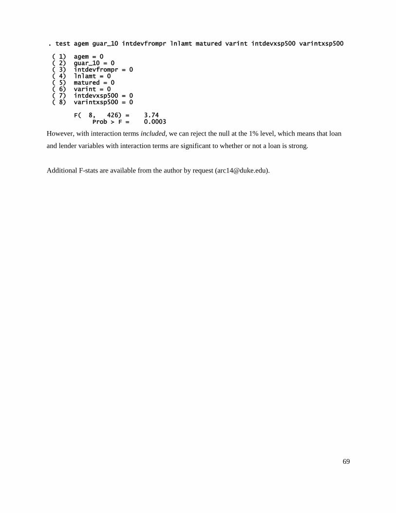
69

However, with interaction terms included, we can reject the null at the 1% level, which means that loan

and lender variables with interaction terms are significant to whether or not a loan is strong.

Additional F-stats are available from the author by request (arc14@duke.edu).

Prob > F = 0.0003 F( 8, 426) = 3.74

( 8) varintxsp500 = 0 ( 7) intdevxsp500 = 0 ( 6) varint = 0 ( 5) matured = 0 ( 4) lnlamt = 0 ( 3) intdevfrompr = 0 ( 2) guar_10 = 0 ( 1) agem = 0

. test agem guar_10 intdevfrompr lnlamt matured varint intdevxsp500 varintxsp500

70

References

Akhavein, J., Frame, W., & White, L. (2001). The Diffusion of Financial Innovations: An Examination of

the Adoption of Small Business Credit-scoring by Large Banking Organizations. Journal of Business,

78(2), 577-596.

Benjamin, L., Rubin, JS. & Zielenbach S. (2004). Community development financial institutions: Current

issues and future prospects.” Journal of Urban Affairs, 26 (2), 177-195.

Berger, A., Frame, W., & Miller, N. (2002). Credit-scoring and the Availability, Price, and Risk of Small

Business Credit. FRB of Atlanta Working Paper No. 2002-6, FEDS Working Paper No. 2002-26.

Berger, A., & Barrera, M. (2007). Credit-scoring for Microenterprise Lenders. Microenterprise Fund for

Innovation, Effectiveness, Learning, and Dissemination. [http://accionnm.org/PDF/CreditScoring.pdf,

Retrieved on April 5, 2010.]

Bhatt, N., & Tang, S. (2001). Making Microcredit Work in the United States: Social, Financial, and

Administrative Dimensions. Economic Development Quarterly, 229-240.

Claire, D., & Kossmann, R. (2003). Credit-scoring: Is It Right for Your Bank? Bannock Consulting.

[http://www.microfinancegateway.org/gm/document-1.9.25232/3702_03702.pdf, Retrieved January 26,

2010.]

Claire, D., Batron, S., de Zubiria, A., Alexiev, Z., Dyer, J., Bundred, F., & Brislin, N. (2006). A

Handbook For Developing Credit-scoring Systems in a Microfinance Context.

[http://www.microlinks.org/ev_en.php?ID=13456_201&ID2=DO_TOPIC, Retrieved on April 5, 2010.]

71

Cowan, C. & Cowan, A. (2006). A Survey Based Assessment of Financial Institution Use of Credit-

scoring for Small Business Lending. Office of Advocacy, U.S. Small Business Administration. Retrieved

September 15, 2009.

Dellien, H., & Schreiner, M. (2005). Credit-scoring, Banks, and Microfinance: Balancing High-Tech with

High-Touch. [http://www.microfinance.com/English/Papers/Scoring_High_Tech_High_Touch.pdf,

Retrieved on February 2, 2010.]

Easton, T. (2005, November 3). The hidden wealth of the poor. The Economist. Retrieved September 2,

2009.

Frame, W., Srinivasan, A., & Woosley, L. (2001). The Effect of Credit-scoring on Small Business

Lending. Journal of Money, Credit and Banking, 33(3), pp. 813-825.

Gerschick, J. (2002). Credit Evaluation Grids for Microlenders: A Tool For Enhancing Scale and

Efficiency. Microenterprise Fund for Innovation, Effectiveness, Learning, and Dissemination.

[http://www.fieldus.org/publications/CEGAccion.pdf, Retrieved on April 5, 2010.]

Glennon, D., & Nigro, P. 2005. “An Analysis of SBA Loan Defaults by Maturity Structure.” Journal of

Financial Services Research. Vol 28, No. 1/2/3, pp. 77-111.

Glennon, D., & Nigro, P. (2005). Measuring the Default Risk of Small Business Loans: A Survival

Analysis Approach. Journal of Money, Credit, and Banking. Vol. 37, No. 5, pp. 923-47.

72

Gokhale, K. (2009, August 13). A Global Surge in Tiny Loans Spurs Credit Bubble in a Slum. Wall Street

Journal. Retrieved September 2, 2009.

Green, R. (2000). Biased Based Lending. Business Week Online.

[http://www.businessweek.com/smallbiz/0005/fi3682082.htm] Retrieved September 29, 2009.

Hermes , N., & Lensink, R. (2007). The empirics of microfinance: what do we know? Economic Journal,

117, F1-F10.

Jensen, R. & Miller, N. (2008). Giffen Behavior and Subsistence Consumption. American Economic

Review, 98(4), 1553-1577.

Keifer, N. (1988.) Economic Duration Data and Hazard Functions. Journal of Economic Literature 26,

646-679.

Krauss, N. & Walter, I. (2008.) Can Microfinance Reduce Portfolio Volatility? Economic Development

and Cultural Change, 58, 85–110.

Mester, L. (1997, September).What's the point of credit-scoring? Business Review, Federal Reserve Bank

of Philadelphia, 3-16.

Morduch, J. (1999). The Microfinance Promise . Journal of Economic Literature, 37(4), 1569 1614.

Oppenheim, S. (November 18, 1996). Would Credit-scoring Backfire in a Recession? American Banker,

pg. 16.

73

Ou, C. (2005). Banking Consolidation and Small Business Lending: A Review of Recent Research

(working paper). Office of Advocacy, U.S. Small Business Administration. Retrieved September 15, 2009.

Overstreet, G., & Rubin, G. (1996). The Applicability of Credit-scoring in Credit Unions. Filene Research

Institute. [http://filene.org/publications/detail/the-applicability-of-credit-scoring-in-credit-unions,

Retrieved on January 26, 2010.]

Painter, G., & Tang, SY. (2001). The Microcredit Challenge: A Survey of Programs in California Journal

of Developmental Entrepreneurship, 6(1), 1-16.

Paxton, J., Graham, D., & Thraen, C. (2000). Modeling Group Loan Repayment Behavior: New Insights

from Burkina Faso . Economic Development and Cultural Change, 48(3), 639-655.

Petersen, Mitchell & Rajan, R. (1994). The Benefits of Lending Relationships: Evidence from Small

Business Data. The Journal of Finance. Vol 94. No. 1, pp. 3-37.

Schall, R. (2003). Raising the Bar: Achieving Scale and Sustainability in Microlending in the United

States . Fleichman Civil Society Fellowship Terry Sanford Institute for Public Policy Duke

University.[http://www.sanford.duke.edu/centers/civil/papers/schall.pdf].

Schreiner, M. (2001). Do-It-Yourself Microfinance Scoring Trees.

[http://www.microfinance.com/English/Papers/Do_It_Yourself_Scoring_Tree.pdf, Retrieved on February

2, 2010.]

74

Schreiner, M. (2004). Benefits and Pitfalls of Statistical Credit-scoring for Microfinance.

[http://www.microfinance.com/English/Papers/Scoring_Benefits_Pitfalls.pdf, Retrieved on January 26,

2010.]

Schreiner, M. (2005). Can Scoring Help Attract Profit-Minded Investors to Microcredit?

[http://www.microfinance.com/English/Papers/Scoring_Helps_Attract_Profit_Minded_Investors_to_Micr

ocredit_Presentation.pdf, Retrieved on February 2, 2010.]

Wenner, M. (2005). Group Credit: A Means to Improve Information Transfer and Loan Repayment

Performance . Journal of Development Studies, 32(2), 264-81.

Yunus, M. (2003). Banker to the Poor: Microlending and the Battle Against World Poverty. New Work,

Public Affairs.