MEASURING THE EFFECT OF PUBLIC LABOR EXCHANGE (PLX ...
274
MEASURING THE EFFECT OF PUBLIC LABOR EXCHANGE (PLX) REFERRALS AND PLACEMENTS IN WASHINGTON AND OREGON Final Report of the Public Labor Exchange Performance Measures Validation Project Prepared under Contract No. X-6879-8-00-80-30 Prepared for: Washington State Employment Security Department 212 Maple Park Olympia, Washington 98504 Prepared by: Louis Jacobson Ian Petta Westat 1650 Research Boulevard Rockville, Maryland 20850-3195 October 4, 2000
Transcript of MEASURING THE EFFECT OF PUBLIC LABOR EXCHANGE (PLX ...

MEASURING THE EFFECT OF PUBLIC LABOR EXCHANGE (PLX)REFERRALS AND PLACEMENTS IN WASHINGTON AND OREGON
Final Report of thePublic Labor Exchange Performance Measures Validation Project
Prepared under Contract No. X-6879-8-00-80-30
Prepared for:
Washington State Employment Security Department212 Maple Park
Olympia, Washington 98504
Prepared by:
Louis Jacobson
Ian Petta
Westat1650 Research Boulevard
Rockville, Maryland 20850-3195
October 4, 2000

iii
TABLE OF CONTENTS
Chapter Page
ACKNOWLEDGEMENTS............................................................................. ix
EXECUTIVE SUMMARY ............................................................................. xi
1 INTRODUCTION AND BACKGROUND..................................................... 1-1
1.1 Overview of PLX Operations ............................................................. 1-21.2 Context for this Study......................................................................... 1-5
2 MEASURING THE RETURNS TO PLX DIRECT PLACEMENTSERVICES....................................................................................................... 2-1
2.1 Measures Based on a Mail Survey...................................................... 2-2
2.1.1 Summary of Key Findings from the Mail Survey............... 2-6
2.2 Measures Based on Administrative Data Alone ................................. 2-9
2.2.1 Summary of the Washington Results .................................. 2-112.2.2 Summary of the Oregon Results ......................................... 2-13
2.3 Concluding Remarks........................................................................... 2-15
3 DETAILS OF OUR RESEARCH USING THE WASHINGTON STATEMAIL SURVEY .............................................................................................. 3-1
3.1 Design of the Survey........................................................................... 3-13.2 Implementation of the Design............................................................. 3-43.3 Improving the Mail Response Rate .................................................... 3-53.4 Differences between Responders and Nonresponders ........................ 3-73.5 Design of the Analysis........................................................................ 3-93.6 Estimators Used in the Analysis ......................................................... 3-143.7 Empirical Analysis.............................................................................. 3-173.8 Placement Effects for Job Seekers with Strong and Spotty Work
Records ............................................................................................... 3-22
3.8.1 Referral Outcomes for Individuals with Spotty WorkRecords................................................................................ 3-24
3.8.2 Referral Outcomes for Individuals with Strong WorkRecords................................................................................ 3-27
3.9 Summary of Reductions in Weeks-Unemployed Due to PLXPlacements .......................................................................................... 3-29

iv
TABLE OF CONTENTS (continued)
Chapter Page
3.10 Translating Weeks Unemployed to Total Benefits ............................. 3-323.11 Summary and Conclusions ................................................................. 3-34
4 DETAILS OF OUR RESEARCH USING WASHINGTON STATE ADMINISTRATIVE DATA ........................................................................... 4-1
4.1 Design of the Analysis........................................................................ 4-34.2 Specification of the Model.................................................................. 4-64.3 Results for All Years Together ........................................................... 4-9
4.3.1 Referral and Placement Effects on UnemploymentDuration .............................................................................. 4-9
4.3.2 Referral and Placement Effects on Weeks of UIPayments ............................................................................. 4-12
4.3.3 Total Benefits of Referrals and Placements ........................ 4-144.3.4 Sensitivity Tests .................................................................. 4-184.3.5 Other Evidence Bearing on the Effectiveness of PLX
Services ............................................................................... 4-20
4.4 Results for Each Year ......................................................................... 4-22
4.4.1 Per-Person Effects by Year ................................................. 4-224.4.2 Number of Claimants Referred and Placed Each Year ....... 4-254.4.3 Total Benefits and Costs by Year........................................ 4-27
4.5 Summary and Conclusions ................................................................. 4-31
5 DETAILS OF OUR RESEARCH USING OREGON ADMINISTRATIVEDATA .............................................................................................................. 5-1
5.1 Database Development ....................................................................... 5-1
5.1.1 Lessons for Developing Analytic Files ............................... 5-3
5.2 The Per-Incident Effect of Referrals and Placements......................... 5-55.3 Estimating Total Benefits ................................................................... 5-7
5.3.1 Measuring the Incidence of Referrals and Placements ....... 5-95.3.2 Estimates of Total Benefits ................................................. 5-145.3.3 Why Total Benefits Differ between Oregon and
Washington ......................................................................... 5-17
5.4 Summary and Conclusions ................................................................. 5-19

v
TABLE OF CONTENTS (continued)
Chapter Page
6 CROWDING-OUT EFFECTS OF THE PUBLIC LABOR EXCHANGEIN WASHINGTON STATE............................................................................ 6-1
6.1 Introduction......................................................................................... 6-16.2 Description of the Model .................................................................... 6-2
6.2.1 Overview............................................................................. 6-26.2.2 Workers............................................................................... 6-46.2.3 Discussion ........................................................................... 6-66.2.4 Firms ................................................................................... 6-66.2.5 Equilibrium ......................................................................... 6-86.2.6 Why Use an Equilibrium Search and Matching Model?..... 6-10
6.3 Implementing the Model..................................................................... 6-116.4 Results................................................................................................. 6-14
6.4.1 Reference Case.................................................................... 6-146.4.2 Variation in the Separation Rate (s) and Ratio of
Vacancies to Unemployed (V/U) ........................................ 6-17
6.5 Summary and Discussion.................................................................... 6-19
7 SUMMARY AND CONCLUSIONS .............................................................. 7-1
7.1 Study 1: Information from the Washington State Mail Survey .......... 7-17.2 Study 2: Information from Washington State Administrative
Data..................................................................................................... 7-47.3 Study 3: Information from Oregon Administrative Data.................... 7-67.4 Estimation of Benefit-Cost Ratios ...................................................... 7-77.5 Study 4: Crowding-Out Effects .......................................................... 7-107.6 Summary of the Strengths and Weaknesses of our Estimation
Techniques.......................................................................................... 7-107.7 Monitoring and Improving Ongoing PLX Operations........................ 7-137.8 Routinely Producing the Measures Described in this Report ............. 7-167.9 Concluding Remarks........................................................................... 7-18
8 THE EXPERT PANEL’S REVIEW................................................................ 8-1
8.1 Introduction......................................................................................... 8-18.2 Description of Panel Members ........................................................... 8-18.3 Westat’s Letters .................................................................................. 8-2

vi
TABLE OF CONTENTS (continued)
Chapter Page
8.3.1 The Initial Letter ................................................................. 8-38.3.2 The Followup Letter............................................................ 8-5
8.4 Expert Panel’s Comments................................................................... 8-6
8.4.1 Comments by Jeffrey Smith................................................ 8-68.4.2 Comments by Burt Barnow................................................. 8-128.4.3 Comments by Daniel Sullivan ............................................ 8-168.4.4 Comments by Stephen Woodbury....................................... 8-20
8.5 Summary of the Comments of All Four Panelists .............................. 8-25
8.5.1 Use of a Natural Experiment to Measure PlacementEffects ................................................................................. 8-26
8.5.2 Use of Nonexperimental Methods to Measure Placementand Referral Effects............................................................. 8-27
8.5.3 Estimation of Displacement Effects.................................... 8-288.5.4 Overall Benefit-cost Computations..................................... 8-298.5.5 Use of the Information to Improve Performance
Measures ............................................................................. 8-308.5.6 Tone of the Report .............................................................. 8-31
8.6 Implications for Future Analysis ........................................................ 8-31
REFERENCES ................................................................................................ R-1
List of Appendixes
Appendix
A Survey Instrument............................................................................................ A-1
B Details of Regression Equation and Variables................................................. B-1
C List of Variables and Regression Estimates--Washington State...................... C-1
D List of Variables and Regression Estimates--Oregon State ............................. D-1
vii
TABLE OF CONTENTS (continued)
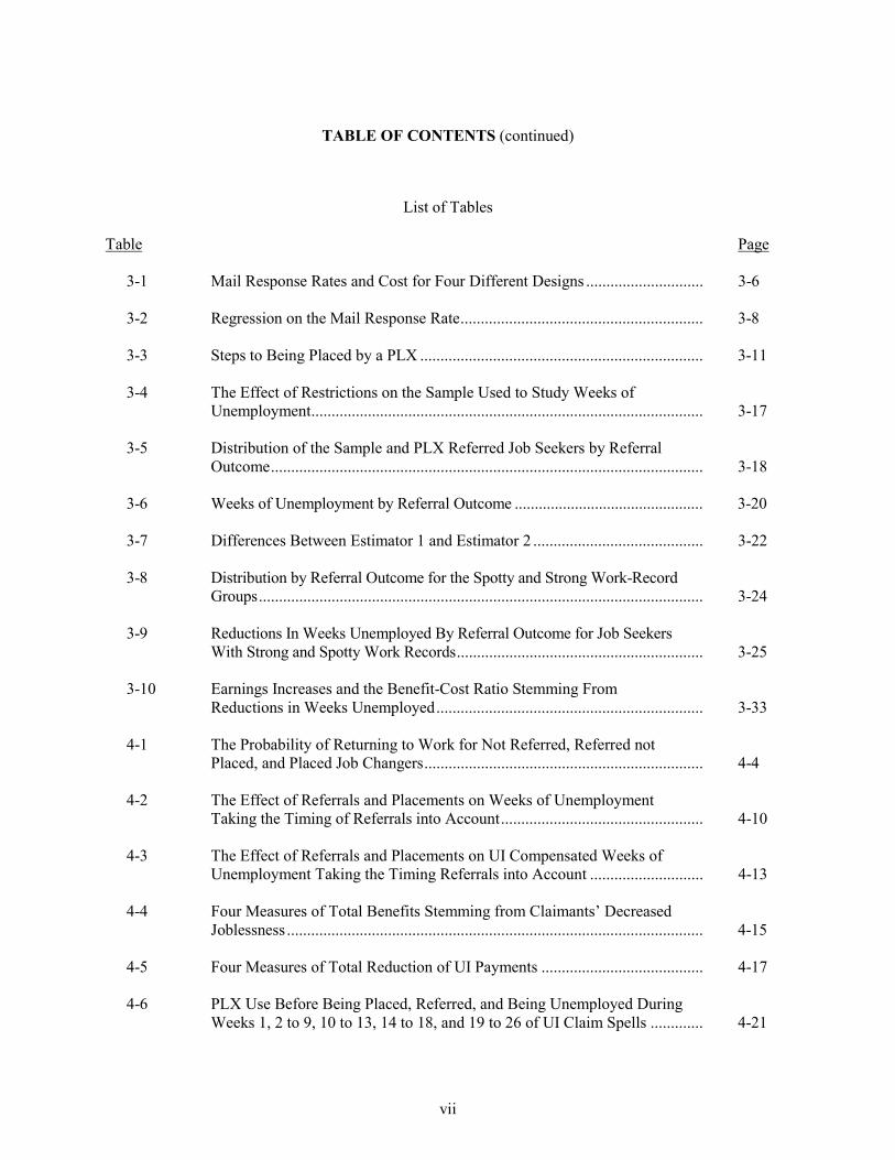
List of Tables
Table Page
3-1 Mail Response Rates and Cost for Four Different Designs ............................. 3-6
3-2 Regression on the Mail Response Rate............................................................ 3-8
3-3 Steps to Being Placed by a PLX ...................................................................... 3-11
3-4 The Effect of Restrictions on the Sample Used to Study Weeks ofUnemployment................................................................................................. 3-17
3-5 Distribution of the Sample and PLX Referred Job Seekers by ReferralOutcome........................................................................................................... 3-18
3-6 Weeks of Unemployment by Referral Outcome ............................................... 3-20
3-7 Differences Between Estimator 1 and Estimator 2 .......................................... 3-22
3-8 Distribution by Referral Outcome for the Spotty and Strong Work-RecordGroups.............................................................................................................. 3-24
3-9 Reductions In Weeks Unemployed By Referral Outcome for Job SeekersWith Strong and Spotty Work Records............................................................. 3-25
3-10 Earnings Increases and the Benefit-Cost Ratio Stemming FromReductions in Weeks Unemployed.................................................................. 3-33
4-1 The Probability of Returning to Work for Not Referred, Referred notPlaced, and Placed Job Changers..................................................................... 4-4
4-2 The Effect of Referrals and Placements on Weeks of UnemploymentTaking the Timing of Referrals into Account.................................................. 4-10
4-3 The Effect of Referrals and Placements on UI Compensated Weeks ofUnemployment Taking the Timing Referrals into Account ............................ 4-13
4-4 Four Measures of Total Benefits Stemming from Claimants’ DecreasedJoblessness ....................................................................................................... 4-15
4-5 Four Measures of Total Reduction of UI Payments ........................................ 4-17
4-6 PLX Use Before Being Placed, Referred, and Being Unemployed DuringWeeks 1, 2 to 9, 10 to 13, 14 to 18, and 19 to 26 of UI Claim Spells ............. 4-21

viii
TABLE OF CONTENTS (continued)
List of Tables (continued)
Table Page
4-7a Effects of Placements and Referrals on UI Payments for Each Year1987 to 1995 .................................................................................................... 4-23
4-7b Effects of Placements and Referrals on Weeks of Unemployment forEach Year 1987-1995 ...................................................................................... 4-23
4-8 Number and Distribution of Referrals, Placements, and Claimants;Comparison of Claimants in the Database to UI First Payments for EachYear 1987 to 1995............................................................................................ 4-26
4-9a Total Yearly Gains from Referrals and Placements ReducingUI Payments..................................................................................................... 4-28
4-9b Total Yearly Earning Gains from Referrals and Placements ........................... 4-28
4-9c Total Yearly Costs and Benefit-Cost Ratios .................................................... 4-28
5-1 Effects of Referrals and Placements on Weeks of Unemployment and UIPayments Sample Size and Percent Referred and Placed, for Five Periodsand Average for all Periods Together, Oregon 1995. ...................................... 5-6
5-2 Claimants and Claimants Referred and Placed Measured with PublishedStatistics and Tabulations of Person-level Files, Oregon and Washington1995. ................................................................................................................ 5-10
5-3 Selected Statistics Describing Direct Placement Services and Job OrderCharacteristics in Washington and Oregon from July 1997 throughJune1998 and Labor Force Characteristics for 1990. ...................................... 5-13
5-4 Estimates of Total Benefits Due to 1995 Referrals and Placements ofClaimants in Oregon and Washington ............................................................ 5-15
6-1 Descriptive Statistics of Public Labor Exchange (PLXs) Registrants,and Estimated Impacts of the PLXs, Washington State, 1987-1995 ............... 6-12
6-2 Simulated Impacts of PLXs on Unemployment Duration, Employment,and the Total Unemployment Rate, Washington State, for VariousSeparation rates (s) and Elasticities of Search Effort (β)................................. 6-15

ix
TABLE OF CONTENTS (continued)
List of Tables (continued)
Table Page
6-3 Simulated Impacts of PLXs on Unemployment Duration, Employment,and the Total Unemployment Rate, Washington State for VariousSeparation Rates (s) and Vacancies per Unemployed Worker (V/U).............. 6-15
7-1 Benefit Cost Ratio............................................................................................ 7-9
List of Figures
Figure
3-1 How referral-outcome groups are organized to produce Estimators 1 & 2 ..... 3-16
6-1 The labor market.............................................................................................. 6-7
6-2 Employment dynamics for type j workers ....................................................... 6-9
8-1 Flow Diagram of Employment Service Participation, with Estimators ofthe Impact of ES Activities Illustrated............................................................. 8-22

xi
ACKNOWLEDGEMENTS
An unusually large number of people merit our thanks for helping make this project possible and assistingus with the work.
First, and foremost, we would like to thank several individuals in the United States Employment ServiceOffice of the Employment and Training Administration, U.S. Department of Labor. We are deeplyindebted to Dave Balducchi for outstanding guidance and patience. Alison Pasternak also greatly assistedus in developing the research. Dave Morman was instrumental in seeing the potential value of this work.Finally, John Beverly, Tim Sullivan, and Jim Vollman all provided useful insights and encouragement.
We cannot praise the efforts of Jeff Jaksich of the Washington State Employment Security Department(ESD) too strongly. He made enormous contributions to our work by making it possible for us to obtainall sorts of assistance from officials in Washington State, and making sure that we were able to secureseveral different types of Washington data. Last, but certainly not least, he worked tirelessly to ensure thatour relations with ETA remained on an even keel
Many other individuals in ESD also provide valuable support, ideas, and encouragement. Theseindividuals include Dr. Russ Lidman and Dr. Greg Weeks, Deanna Cook, and Barbara Flaherty. Othersdeserve special thanks for helping to provide various forms of data. These individuals include PeterSyben, Judy Barney, Kay Kaliman, Chey Kyarky, and Lorrie Como.
Similarly, we benefited greatly from the assistance of many of individuals at the Oregon EmploymentDepartment (OED). The support and advice of Virlena Crosley, OED Director, was an essential elementof this work. We also greatly benefited by the efforts of Tom Lynch and his colleagues in creating theOregon data warehouse. Patrick McIntire played a central role in ensuring that we had the information weneeded about the Oregon PLXs and that the databases met our needs. John Glen made major contributionsby running innumerable versions of our models. We also are especially indebted to Bryan Conway andAlyson Mah for creating the initial file to our specifications, and to Saleem Ahmad and Chuck Oswalt tohelping deal with data anomalies as they arose. We also appreciate the help provided by Eric Moore andTracy Louden. Many individuals provided tremendous help in ensuring that the data we needed wasproperly formatted.
We also greatly benefited by the excellent work by a panel of technical experts who reviewed our work,and provided many penetrating comments about how the analysis should be improved. The expert panelincluded Burt Barnow, Johns Hopkins University; Arnold Katz, University of Pittsburgh; Bob LaLonde,University of Chicago; Jeff Smith, the University of Western Ontario; Dan Sullivan, Federal ReserveBank of Chicago; and Steve Woodbury, Michigan State University and the Upjohn Institute. We alsogreatly appreciate that Dr. Woodbury drafted Chapter 6 with the help of Carl Davidson, his colleague atthe Michigan State University.
Finally, we greatly appreciate the aid provided by Ginny Baldwin, an independent editor, and the editorialassistance of Arlene Shykind and her staff at Westat. We also acknowledge the assistance of many of ourcolleagues at Westat including Regina Yudd, Andrea Wilson, Ellen Tenenbaum, and Alex Ratnofsky.
Despite all of the above people’s best efforts, any remaining errors in the work are the principal author’sresponsibility. Also, the opinions expressed are solely those of the authors.

Executive Summary

xiii
EXECUTIVE SUMMARY
This report describes our analyses of the effects of direct placement services provided bypublic labor exchanges (PLXs) to job seekers in the states of Washington and Oregon from 1987 to 1998.A nationwide system of state-Federal PLXs was created following passage of the Wagner–Peyser Act in1933. Our goal was to determine their value and develop procedures that the U.S. Department of Labor(US-DOL) could routinely use to provide meaningful feedback to PLX program operators and state andFederal policymakers.
Overview of Our Findings on the Benefits and Costs of PLX Services
The primary focus of our work was to develop a means to accurately measure the returns todirect placement services—referrals and placements. To do this we relied on three data sets:
1. Survey responses from 587 job seekers referred to jobs by Washington State PLXs during thefirst half of 1998.
2. Administrative data covering PLX use during 328,815 spells of unemployment covered byunemployment insurance (UI) in Washington State from 1987 through mid-1995.
3. Administrative data covering PLX use during 138,280 spells of unemployment covered by UI inOregon during 1995.
We used these data to estimate the effect of placements and referrals on the duration ofunemployment. We also used a simulation model developed by Professors Davidson and Woodbury ofMichigan State University to examine the extent to which reductions in unemployment to PLX userscomes at the expense of nonusers.
Estimating the effect of PLX services is a very difficult task because the effects of these servicesper person are often small and because random assignment (experimental) designs cannot be used.Technical experts agree that experimental designs offer the best means to produce unbiased estimates, butPLXs must provide universal access, making it impossible to implement those designs. Thus, much of ourwork was aimed at finding alternative ways to produce results that an expert panel would agree are

xiv
unbiased. While we had some success in finding ways around the central problem, we did not have timeto fully implement the solutions. Thus, our estimates of direct placement effects substantially narrow therange of plausible values, rather than provide tight point estimates.
Our primary conclusion from our analyses is that surveys have the potential to identifyjob seekers referred to jobs too late to obtain interviews, and that these individuals would serve as acomparison group to produce unbiased estimates of placement effects—the value of being placedrelative to obtaining referrals.
The pilot procedures tested in this report produced estimates that job seekers with strongwork records in our sample who were placed by PLXs experienced a 7.2-week reduction in their durationof unemployment, and placed job seekers with spotty work records experienced a 3.4 week reduction.These unemployment reductions translate into increases in earnings of $1,872 and $684 for job seekerswith strong and spotty work records, respectively.
If we make the highly conservative assumption that placements are the only source ofbenefits from PLXs, placements must return more than $542, on average, for PLXs to be cost effective.The placements included in our sample returned about $978, on average. This calculation produces arespectable benefit-cost ratio of 1.8 for the sample studied.
Unfortunately, we cannot legitimately claim that the results generated from our pilot sampleapply to all 11,144 claimants and 35,038 nonclaimants placed by Washington State PLXs in 1998. Theprimary problem is that the pilot sample was not representative of all placements. There also is someuncertainty about how close our unemployment reduction estimates are to the true values for those in thesample. This is because the small sample we used produced relatively large confidence intervals, andsome bias may have been introduced because some job seekers in our comparison group may have beendenied interviews because employers felt they were unsuitable. Fortunately, all three problems could beeliminated in future work by surveying a large representative sample and obtaining additional informationabout the reason for being unable to secure interviews.
A second important conclusion is that, once we have unbiased measures of placement-effects based on identifying job seekers who obtained referrals too late to secure interviews, thoseestimates can be used as benchmarks to produce unbiased results from administrative data alone.

xv
Indeed, even though our survey-based estimates of placement effects are not definitive, thoseresults for UI claimants were similar to those derived from analysis of the very large administrativedatabases for Washington State, especially when differences in business conditions are taken intoaccount. The administrative data showed that benefits are about 30 percent greater in the trough of abusiness cycle than during its peak because there are fewer claimants to help in good times, and claimantscan more readily find jobs on their own in prosperous periods. Thus, much of the differences observedcould be attributed to business conditions being substantially better in 1998 than during the 1987-95period covered by the administrative data.
We believe that the differences between the survey-based and administrative-data-basedresults were small for two reasons. First, the comparisons used to measure placement effects are restrictedto job seekers referred to jobs. Thus, selection bias due to only some job seekers choosing to use PLXs isabsent from these estimates. Usually this is the largest source of bias and the one that is most difficult toremove. Second, we speculate that only small biases were introduced due to the survey sample beingnonrepresentative and some job seekers in the comparison group being rejected by employers
A third key conclusion is that placement-effect estimates substantially underestimatethe total value to job seekers of direct placement services. Our estimates based on administrative dataalone suggest that placement reduce claimants’ unemployment by 7.7 weeks, while referrals not leadingto placements reduce claimants’ unemployment by 2.1 weeks. Because only about 1 in 5 claimantsobtaining referrals are placed, even small per-person gains due to referrals not leading to placementswould produce large benefits in total. Estimates based on administrative data suggest that about 55percent of earnings gains come from placements, and 45 percent come from obtaining information fromuse of job banks and staff in the course of being referred.
Because we lack an unbiased estimate of referral effects for use as a benchmark we do notknow how close our referral-effect estimates are to the true effects. However, we do know that referraleffects estimates depend on comparing PLX-users to nonusers, and that selection bias in these types ofcomparisons consistently leads to underestimation of the true effect. In general, individuals volunteeringto use government services have special difficulties that make them need the aid more than nonusers, butthe factors that are associated with these differences often are not described well with available data.
Indeed, referral effects were zero prior to adjusting the raw differences between referredclaimants and those not referred to account for selection bias. Also, experimental evidence on the effect ofjob search assistance (JSA) uniformly suggests that JSA has small positive effects. However, we believe

xvi
that PLX direct placement services are considerably more potent than the types of JSA studied usingexperimental designs. We, therefore, are confident that the true effect is considerably greater than zero,even if it is not as great as the 2.2-week estimate we produced. Thus, we feel that it is reasonable tobelieve that there are substantial benefits derived from obtaining referrals, even when jobs are ultimatelylocated from other sources.
Clearly, obtaining unbiased referral-effect estimates for use as a benchmark is of enormousimportance in estimating the value of PLX direct placement services with accuracy. Obtaining such abenchmark is difficult because it is not feasible to create a control group by denying access to PLX job-listings. However, it may be possible to develop unbiased benchmarks from an experimental design thatwould randomly call in claimants to review job listings. Although we could not prevent job seekers whowere not called in from using PLX services voluntarily, we still could measure the bias associated withusing nonexperimental estimators. Also, it may be possible to develop a reasonable estimate of referraleffects based on experimental evidence of the value of job search assistance programs that do not requiregranting universal access.
A fourth key conclusion is that the per-person placement and referral effects forclaimants in Oregon were considerably smaller than the effects in Washington State. Oregonadministrative data suggest that placements reduced claimants’ duration of unemployment by 4.6 weeks,and referrals not leading to placements reduced claimants’ duration of unemployment by 1.1 weeks. Eventhough we have no unbiased estimates for use as benchmarks, we feel that it is reasonable to believe thebiases in the Oregon and Washington results are similar. Thus, the differences in the results are primarilydue to differences in the true effects.
These differences could stem from two key differences in the way claimants interact withPLXs in the two states. First, Oregon applies a more stringent work test and requires claimants to registerwith PLXs in person, where they are likely to also review PLX job listings. These actions makes it morelikely that Oregon claimants who do not obtain PLX aid will quickly accept suitable jobs or stop claimingbenefits, and those who examine listings will also quickly find jobs and pursue leads they develop ontheir own more vigorously. Second, Oregon spends more state funds on PLXs than does Washington,even though both states substantially boost expenditures above those provided by Federal programs. Thehigher spending in Oregon translates to more job orders available per PLX user in Oregon. Having morejob orders per person also allows Oregon to refer and place about the same number of clients asWashington, despite having about half as many jobs available overall in Oregon as in Washington.

xvii
We suspect that the combination of claimants viewing listings early in their spells ofunemployment and having more openings to choose from helps claimants who, on average, are morelikely to find jobs quickly on their own. Certainly, the administrative data in both states shows that theper-person effects of direct placement services are far greater after the tenth week of unemployment. Wecould test these hypotheses more definitively by combining the data from the two states. However, thatwas not possible in this study because Oregon could not release its data to us, and we lacked the time totransfer the Washington data to Oregon.
Our fifth conclusion is that PLX direct placement services substantially reduce UIpayments. However, these reductions equal about one-quarter of the gains in earnings. Thisevidence rests on estimates that use administrative data alone. However, we suspect that there is little biasin the estimate of the split between reductions in total unemployment, which raise job seekers’ earnings,and unemployment covered by UI payments, which reduce UI payouts. Importantly, employers often onlyfocus on the direct benefits of reductions in UI payroll taxes owing to reductions in UI payouts. However,they often overlook that they also benefit directly from vacancies being filled more quickly. Similarly,they often overlook that they benefit indirectly from being able to reduce wages they must pay theirworkers to compensate them for the risk of job loss and temporary unemployment stemming from PLXsmaking these situations less costly to job seekers.
Our final key result is that 80 percent of the benefits to claimants were derived fromhelping employers fill vacancies more quickly. This directly leads to expanding the production of goodsand services and reducing their price. The simulation model we used also suggested that the negative“crowding-out” effects on nonclients are small per person, equal to only about 2.5 hours of work. As withour other evidence, we do not claim that we proved that the crowding-out effect is exactly 20 percent, butthat the true effect is in the neighborhood of that value.
In summary, our most important achievement is developing a procedure that we areconfident would produce unbiased estimates of placement effects, if fully implemented. Also, wehave developed several additional procedures that might produce unbiased estimates of referral effects.Having measures that technical experts agree are unbiased is of enormous importance because theseestimates could be used as benchmarks for developing measures to use administrative data alone to alsoproduce unbiased estimates.
While technical experts do not agree that our current estimates are unbiased, ourevidence on the effectiveness of direct placement services suggests that the benefits are substantially

xviii
greater than the costs— returning perhaps as much as $2 for each $1 spent. Our best evidence forthis view is that the placement-effect estimates that use the administrative data and survey data inWashington are similar and the bias in these estimates is likely to be relatively small. Also, our analysissuggests that referral effects are considerably greater than crowding out effects. In short, while we do nothave point estimates that experts would agree precisely identify these effects, the estimates we do haveconsiderably narrow the likely range of plausible effects. Importantly, we have outlined additionalanalyses that would further shrink the plausible range of these effects.
Overview of Our Findings on Ways to Improve Monitoring of PLX Activities
Although the primary focus of our work was to develop ways to accurately estimate thebenefits and costs of direct placement services, we also examined the value and feasibility of using themeasures we created to routinely monitor PLX performance. Our central conclusion is that it would behighly feasible to routinely use the measures derived from administrative records because the datarequired are not very different from those needed to implement the measures called for in the WorkforceInvestment Act (WIA).
Of great importance, while the measures are not perfect, they provide information that islikely to help PLX managers and staff substantially increase the value of PLX services, as well asprovide a reasonably accurate view of the total value of PLX services. In particular, the measures weproduce here have the potential to assist in making key decisions about:
When, relative to the start of unemployment spells, claimants should be given PLXservices.
How effort should be divided between securing and filling job orders versus providinglabor market information that can help clients find jobs on their own.
What types of clients benefit the most from placements versus information that helpsfinding jobs on one’s own.
In sharp contrast, maximizing WIA measures, such as the entered employment rate, is likelyto lead to decisions that reduce the value of PLX services. The central problem with WIA measures is thatthey give incentives for PLXs to serve clients most likely to find work on their own rather than clientswho will benefit the most from PLX aid. Importantly, the problems with use of descriptive statistics asperformance measures is much greater for PLXs that grant universal access than for targeted programs

xix
such as those funded under JTPA. Specifically, creaming and other negative consequences of usingmeasures like the entered employment rate were minimized under JTPA because program operators wererequired to enroll clients with substantial impediments to finding jobs on their own.
We learned a great deal about the feasibility of a state agency creating the measures becausethe Oregon Employment Department (OED) did all of the data processing for the Oregon study with littlehelp from us. However, the data processing has to be carefully executed. In particular, the completenessof the coverage of individuals in the raw files needs to be checked against published statistics, and thetransformation of each variable needs to be checked by comparing the input and output files at each stage.
Finally, it is our view that the appropriate criterion for use of the measures in this report iswhether they are superior to other measures. The measures do not need to be perfect in order for them tobe highly useful. At the same time, every effort should be made improve the statistical quality of theestimates. Thus, the additional work outlined in the preceding section would be of substantial value.However, even that work would not be sufficient to measure referral effects accurately usingadministrative data for nonclaimants and to expand the range of PLX services included in the analysis.Producing these measures would further increase the usefulness of the measures. Considerable progress indeveloping those measures could be made using an expanded mail survey that included telephonefollowup.
The major threat to developing a comprehensive measurement system, however, is the rapidspread of PLX computer systems that allow clients viewing listings to obtain contact information withoutstaff intervention. Only in Oregon are self-referrals tracked, but without such tracking, it is almostimpossible to measure the benefits of direct placement services. Thus, the benefits and costs of theOregon system merit careful study. If the analysis is positive, serious consideration should be given torequiring that self-referrals be tracked nationwide.
Details of the Individual Studies
The above sections summarize our overall findings for all four of the studies presented inChapters 3 through 6. The next few sections of the executive summary provide additional information tomake the results and estimation procedures of the individual studies clearer. Additional backgroundinformation about PLX operations, estimation techniques, and results are found in Chapters 1 and 2.Chapter 7 presents an expanded discussion of the issues raised in this overview, and presents more

xx
information about the conceptual framework of our analysis. Chapters 3 through 6 present our work insufficient detail for technical experts to assess the quality of that work independently. Obtaining feedbackfrom experts is important because the accuracy and relevance of the innovative estimation proceduresused need to be independently judged in order for the results to be widely accepted. Chapter 8presents our expert panel’s comments, a summary of areas of agreement and disagreement, andsuggestions for future analysis.
As noted earlier, our primary focus was estimating reductions in unemployment due toreferrals and placements of job seekers with strong work records, most of whom were unemploymentinsurance (UI) claimants, and of job seekers with weak work records. All those benefiting from PLXservices had reached Step 5 on the job search path shown in Table 1. These job seekers had decided tosearch for work (Step 1), decided to obtain assistance from PLXs (Step 2), were able to look at PLX joblistings (Step 3), looked at PLX job listings (Step 4), and found promising listings for which they wantedcontact information (Step 5).
Table 1. Job Search Path from Deciding to Search for Work Through Deciding to Use PLXs toPlacement by a PLX
Steps to surmount Path ending outcomesStep 1. Unemployed worker decided to
search for worka. Recalled by former employerb. Retiredc. Dropped out of labor force
Step 2. Job seeker decided to use PLX No desire to use PLXStep 3. Job seeker gained access to PLX Unable to use PLX because services were
unavailable or too difficult to accessStep 4. Looked at PLX listings Found no suitable jobsStep 5. Found promising listings Decided not to interview for those jobsStep 6. Tried to obtain an interview a. Job or interview slots filled
b. Employer rejected job seeker based onprescreening
Step 7. Obtained interview Did not receive an offerStep 8. Received an offer Rejected offerStep 9. Accepted offer Did not show up for workStep 10. Showed up for work Placed by PLX system

xxi
Our research focused on measuring the value of direct placement services because:
Maintaining a universal system for employers to list job openings and for job seekersto view those openings is the distinguishing feature of PLXs and absorbs most of itscosts;
PLXs’ provision of direct placement services plays a central role in the shift from thegovernment’s “train-first” to “work-first” policy, and it was an opportunity todetermine how well the policy was working; and
Little is known about the value of direct placement services because the requireduniversal access precludes use of a random-assignment design, and devising accuratealternative measurement techniques is extremely difficult.
We examined three benefits of direct placement services to job seekers: (1) gains in earningsattributable to reduced periods of joblessness; (2) reductions in unemployment insurance payments, whichprimarily benefited employers in the form of reduced payroll taxes; and (3) increases in the overallefficiency of the labor market that benefit society at large by expanding the amount of goods and servicesthat are available and by lowering their price.
We focused on two different ways PLXs can assist job seekers. The first is by directlyplacing individuals at jobs listed with the PLXs (Step 10 in Table 1). The second is by providinginformation that helps job seekers find jobs more rapidly on their own or accept jobs to which PLXssupplied referrals (Steps 4 through 9 in Table 1). The benefits of direct placement are obvious. Lessobvious is that looking at listings and obtaining information about job prospects from PLX staff canprovide job seekers with a more realistic assessment of the pay and other characteristics of jobs they arelikely to find on their own and better ways to locate suitable jobs. The literature on job search suggeststhat lack of accurate information is a major impediment to finding work quickly.
Accurate measurement of the effect of referrals and placements hinges on comparing whatactually happened to job seekers receiving those services, which is directly observable, to what wouldhave happened had those services not been received, which is not directly observable. Our researchexplored two alternatives to the use of a random-assignment design for determining what would haveotherwise happened. The first was to take advantage of a natural experiment identified through use of amail survey. When properly used, this information can come close to the ideal of comparing PLX placedjob seekers to job seekers who were identical to those placed except that they were unable to secureinterviews after being referred.
xxii
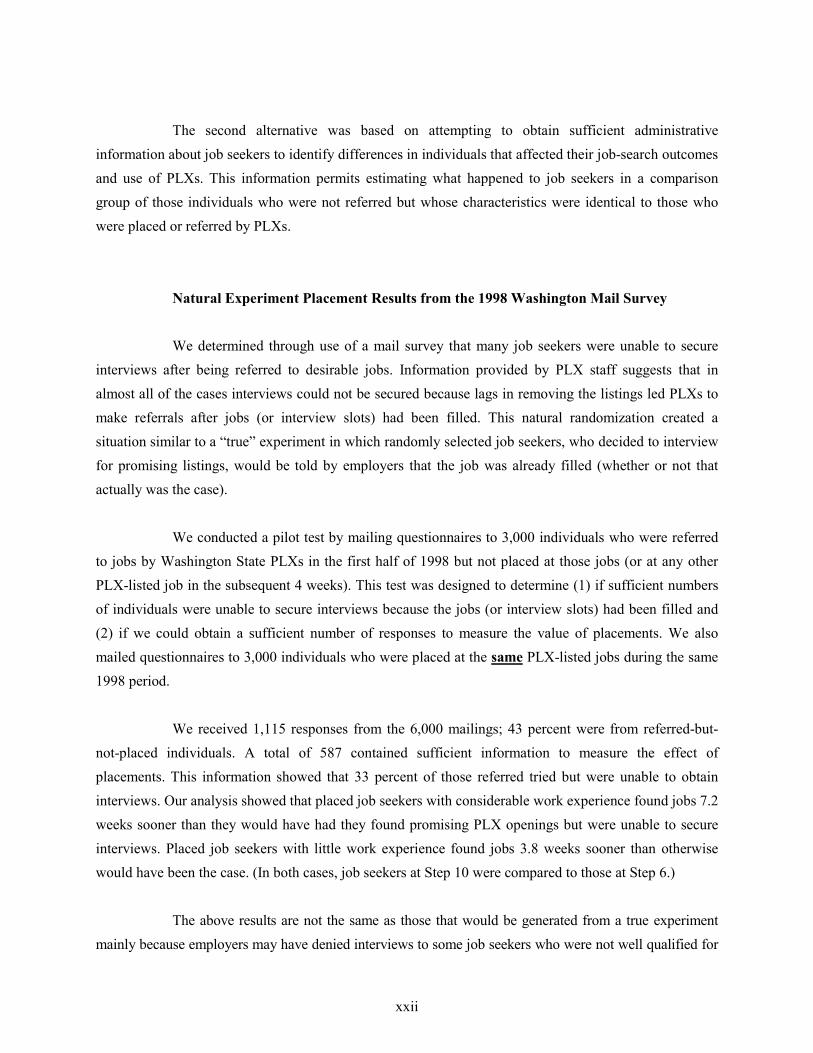
The second alternative was based on attempting to obtain sufficient administrativeinformation about job seekers to identify differences in individuals that affected their job-search outcomesand use of PLXs. This information permits estimating what happened to job seekers in a comparisongroup of those individuals who were not referred but whose characteristics were identical to those whowere placed or referred by PLXs.
Natural Experiment Placement Results from the 1998 Washington Mail Survey
We determined through use of a mail survey that many job seekers were unable to secureinterviews after being referred to desirable jobs. Information provided by PLX staff suggests that inalmost all of the cases interviews could not be secured because lags in removing the listings led PLXs tomake referrals after jobs (or interview slots) had been filled. This natural randomization created asituation similar to a “true” experiment in which randomly selected job seekers, who decided to interviewfor promising listings, would be told by employers that the job was already filled (whether or not thatactually was the case).
We conducted a pilot test by mailing questionnaires to 3,000 individuals who were referredto jobs by Washington State PLXs in the first half of 1998 but not placed at those jobs (or at any otherPLX-listed job in the subsequent 4 weeks). This test was designed to determine (1) if sufficient numbersof individuals were unable to secure interviews because the jobs (or interview slots) had been filled and(2) if we could obtain a sufficient number of responses to measure the value of placements. We alsomailed questionnaires to 3,000 individuals who were placed at the same PLX-listed jobs during the same1998 period.
We received 1,115 responses from the 6,000 mailings; 43 percent were from referred-but-not-placed individuals. A total of 587 contained sufficient information to measure the effect ofplacements. This information showed that 33 percent of those referred tried but were unable to obtaininterviews. Our analysis showed that placed job seekers with considerable work experience found jobs 7.2weeks sooner than they would have had they found promising PLX openings but were unable to secureinterviews. Placed job seekers with little work experience found jobs 3.8 weeks sooner than otherwisewould have been the case. (In both cases, job seekers at Step 10 were compared to those at Step 6.)
The above results are not the same as those that would be generated from a true experimentmainly because employers may have denied interviews to some job seekers who were not well qualified for
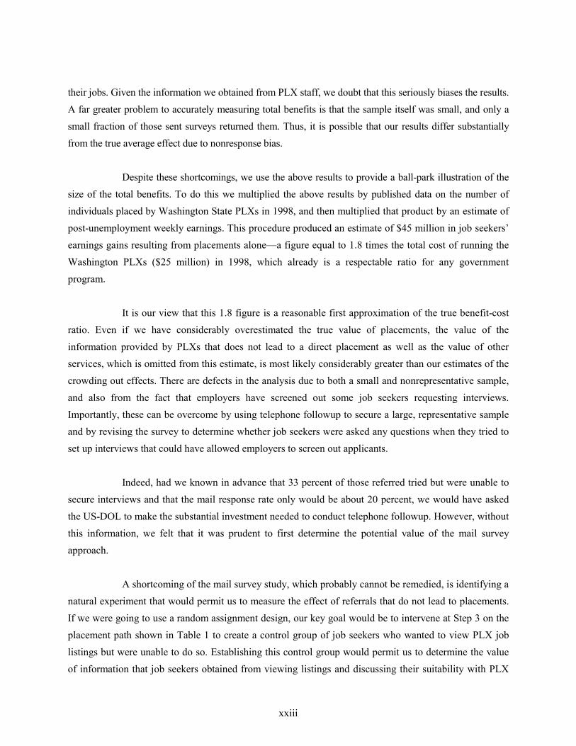
xxiii
their jobs. Given the information we obtained from PLX staff, we doubt that this seriously biases the results.A far greater problem to accurately measuring total benefits is that the sample itself was small, and only asmall fraction of those sent surveys returned them. Thus, it is possible that our results differ substantiallyfrom the true average effect due to nonresponse bias.
Despite these shortcomings, we use the above results to provide a ball-park illustration of thesize of the total benefits. To do this we multiplied the above results by published data on the number ofindividuals placed by Washington State PLXs in 1998, and then multiplied that product by an estimate ofpost-unemployment weekly earnings. This procedure produced an estimate of $45 million in job seekers’earnings gains resulting from placements alone—a figure equal to 1.8 times the total cost of running theWashington PLXs ($25 million) in 1998, which already is a respectable ratio for any governmentprogram.
It is our view that this 1.8 figure is a reasonable first approximation of the true benefit-costratio. Even if we have considerably overestimated the true value of placements, the value of theinformation provided by PLXs that does not lead to a direct placement as well as the value of otherservices, which is omitted from this estimate, is most likely considerably greater than our estimates of thecrowding out effects. There are defects in the analysis due to both a small and nonrepresentative sample,and also from the fact that employers have screened out some job seekers requesting interviews.Importantly, these can be overcome by using telephone followup to secure a large, representative sampleand by revising the survey to determine whether job seekers were asked any questions when they tried toset up interviews that could have allowed employers to screen out applicants.
Indeed, had we known in advance that 33 percent of those referred tried but were unable tosecure interviews and that the mail response rate only would be about 20 percent, we would have askedthe US-DOL to make the substantial investment needed to conduct telephone followup. However, withoutthis information, we felt that it was prudent to first determine the potential value of the mail surveyapproach.
A shortcoming of the mail survey study, which probably cannot be remedied, is identifying anatural experiment that would permit us to measure the effect of referrals that do not lead to placements.If we were going to use a random assignment design, our key goal would be to intervene at Step 3 on theplacement path shown in Table 1 to create a control group of job seekers who wanted to view PLX joblistings but were unable to do so. Establishing this control group would permit us to determine the valueof information that job seekers obtained from viewing listings and discussing their suitability with PLX

xxiv
staff. However, with the possible exception of job seekers living in isolated rural areas, all job seekers caneasily visit PLX offices or view listings using computers at libraries and other public places. Also, jobseekers with access to personal computers in both rural and urban areas can view listings using theInternet.
Not having reliable experimental evidence about the value of referrals that do not lead toplacements is an important shortcoming. First, experimental evidence suggests that job search assistancethat is less intensive than obtaining information from viewing PLX listings and interacting with PLX staffis of substantial value. Second, even a small per-person referral effect would greatly increase total PLXbenefits because four out of five job seekers who obtained referrals were not placed by PLXs.
Nonexperimental Referral and Placement Results for Washington Claimants from1987-95 Administrative Data
Although we could not produce experimental estimates of referral effects, we were able toobtain a plausible range of estimates by applying nonexperimental techniques to PLX administrative data.We did this by comparing the duration of unemployment of job seekers who were referred but not placed(who reached Step 4 in Table 1 but did not reach Step 10) to job seekers who were not referred (did notreach Step 4) and in most cases did not use PLXs at all (did not reach Step 3).
Importantly, we also used the same technique to replicate the estimates derived from thenatural experiment identified with the mail survey to estimate the value of placements (reaching Step 10)relative to obtaining information from the listings and PLX staff (reaching Steps 4 through 9). Theseresults were similar to those generated from the mail survey, which suggests that biases in the techniquesusing the natural experiment and administrative data are reasonably small.
Because administrative data only provide the detailed information needed for this analysisfor UI claimants, we limited the nonexperimental analysis to this one group. In particular, the datadescribe how long claimants have been unemployed when they receive PLX services and, in most cases,when they returned to work. Being able to produce separate estimates based on how long claimants wereunemployed at the point they received PLX aid proved to be a particularly potent way to take into accountfactors that influence PLX use and subsequent duration of unemployment that were not directlyobservable.

xxv
Also of considerable importance, UI claimants are likely to either be reemployed orsearching for work, rather than having retired or dropped out of the labor force. Using these data,therefore, greatly reduces measurement problems stemming from an inability to distinguish betweenjobless individuals who are looking for work and those who are not looking.
Thus, it is reasonable to believe that our analytic technique explicitly or implicitly heldconstant many of the factors that affect job search outcomes, as well as those leading to an individual’sdecision to use PLX services and, thereby, was relatively free of bias. However, as mentioned earlier, wecould not measure the amount of residual bias in our measure of referral effects because we could notcreate a benchmark derived from a random assignment design.
As shown in Table 2, we used administrative data alone covering 1987 through 1995 toestimate that Washington State claimants who were referred but not placed returned to work 2.1 weekssooner than they would have if they had not obtained referrals. As noted earlier, both placed and referred-but-not-placed claimants may benefit from having more accurate information about the difficulty offinding suitable work, as well as from having more opportunities to interview for jobs. Thus, PLX usersmay more quickly accept job offers they obtain on their own or receive as a direct result of PLX referralsthan they would if they had less accurate information about the state of the job market.
Table 2 also displays our estimate that the reduction in joblessness of placed claimants(those reaching Step 10) was 7.7 weeks less than those who were referred-but-not-placed (those reachingsteps 4 though 9). The 7.7-week estimate measures precisely the same benefit source as the 7.2-weekestimate derived from the natural experiment revealed by our mail survey for 1998, but applies to the1987-95 period. Importantly, our year-by-year analysis of the Washington administrative data indicatesthat the effect of being placed in 1987-95, a period strongly affected by recessions, is at least 15 percentgreater than being placed in 1998, a prosperous year.
Applying the 15 percent differential to the 7.2-week estimate suggests that the effect ofbeing placed in 1987-95 would be about 8.3 weeks. Thus, if anything, the nonexperimental estimatorproduces conservative results. Importantly, a direct comparison using the 1998 mail survey and 1998administrative data also suggests that the nonexperimental measures underestimate placement effects.Also, unlike the mail survey results, these results are based on an exceptionally large, representativesample.

xxvi
Table 2. Study Characteristics and Measures of PLX Benefits
Back to work effect of:
Data sourcePopulation
studied
Placementrelative to
referral
Referralrelative tono referral1
Total PLXbenefits per
year2Benefit – costcomparisons3
Study-1WashingtonMail Survey andAdministrativeData for the firsthalf of 1998
A sample of587 individualsreferred to PLXjob openings
7.2 weekssooner for jobseekers withstrong workrecords
3.8 weekssooner for jobseekers withweak workrecords
Notexamined
$45 million forall 1998 PLXusers fromplacementsalone
Annual cost$25 million
Benefit-costratio 1.8
Study-2WashingtonAdministrativeData for1987–95
A sample of328,815 spells ofunemploymentexperienced byUI claimants
7.7 weekssooner
2.1 weekssooner
$11 million forclaimantplacementsalone 1987-95
$25 million forclaimantplacements andreferrals1987-95
Annual cost $25million
35 percent spenton claimants
Benefit-costratio between 1.2and 2.8
Study-3OregonAdministrativeData for1995
A sample of138,280 spells ofunemploymentexperienced byUI claimants
4.6 weekssooner
1.1 weekssooner
$15 million for1995 claimantplacementsalone
$30 million for1995 claimantplacements andreferrals
Annual cost $26million
38 percent spenton claimants4
Benefit-costratio between 1.6and 3.1
1 Referral effects measure the value of information obtained by viewing PLX listings and obtaining staff aid that improves the decisionmaking ofplaced and nonplaced PLX users.
2 Study 1 uses published statistics to estimate the number of placements. Study 2 uses tabulations of person-level files to measure the number ofplacements and referrals. Study 3 uses both sources of information. Use of published data for 1995 raised benefit estimates for Study 2 to $42million for placements and referrals together and $13 million for placements alone. This increased the 1995 benefit-cost ratios to 4.5 forplacements and referral and to 2.1 for placements alone.
3 Benefit-cost ratios are not adjusted for crowding-out effects analyzed in Chapter 6. Their inclusion would reduce the ratios by about 20 percent.4 Only 25 percent of Washington PLX costs went to referring claimants in 1995.

xxvii
If we ignore the value of information obtained in the course of being referred, the totalbenefits in terms of job seekers’ earnings gains are about $11 million per year for 1997-95. This amountequals about 55 percent of the entire yearly cost of running the PLXs. But we estimate that only about 35percent of PLX costs went to helping claimants. Reductions in UI payments to job seekers who wereplaced equaled about $2.6 million per year. Thus, job seekers’ net income gain was about $8.4 millioneach year. However, employers benefited from the reduced UI payouts by having their tax burdenreduced.
The above calculations produce a highly respectable 1.7 benefit-cost ratio. The benefit-costratio was particularly high in the 1991–93 recessionary period because jobs were hard to find, manyclaimants needed help, and UI payments were extended to cover much longer periods than usual. Totalbenefits in today’s economic conditions are considerably less than in 1991–93, mainly because in thisboom time, PLXs are assisting far fewer claimants. Nevertheless, economic conditions in 1990 were notmuch different from today’s, and total benefits accruing to claimants in that year equaled 40 percent ofthe total cost of running the entire PLX system in Washington
If we accept as accurate the 2.2-week estimate of the per-incident value of information notleading to a placement, adding these benefits ($14 million) to those for claimants who were placedincreases average total benefits to about $25 million per year for 1987-95. This is roughly equal to theentire annual cost of running the PLXs. About 55 percent of the benefits are due to placements and theremainder to referrals that do not lead to placements. Placements account for most of the benefits becauseplacement effects are about five times greater than referral effects, even though four times as manyclaimants are referred but not placed, as are placed.
We feel that a careful comparison between our referral effect estimates and existingexperimental evidence on the value of job search assistance would be very useful to determining whetherour 2.2-week estimate is unreasonably high. Our quick review of the differences between PLX servicesstudies here and the types of job search assistance studied using random-assignment designs suggest to usthat the benefits are much closer to $25 million per year than to $11 million. Unfortunately, we lackexperimental evidence that can provide a precise estimate of the effect of measurement bias on ourestimates. Thus, we have presented a plausible range for our estimates.
However, we can further refine our estimates using information from Davidson andWoodbury’s simulation of the effect of PLX services on overall employment and unemployment inWashington State presented in Chapter 6. Their analysis suggests that our 1.7 benefit-cost ratio should be

xxviii
reduced to 1.4. This reduction occurs because about 20 percent of the benefits gained by job seekers whoobtained PLX referrals came from crowding out job seekers who did not obtain referrals but who wouldhave found out about these jobs without PLX aid, secured interviews, and possibly been hired.
This simulation, which used Westat’s measures of PLX effectiveness, also suggests that thecrowding-out effect is dispersed across tens of thousands of workers. The negative effect, therefore, isextremely small per capita, amounting to a loss of about 2.5 hours of work per person. Overall, thepositive effect of PLX activities far outweighs the negative effect and leads to a reduction in the averageduration of job search. This reduction creates a small but measurable increase in employment and adecrease in unemployment. These changes benefit society at large by increasing the total output of goodsand services and benefit employers by helping them fill vacancies more quickly.
In summary, our Washington State analyses suggest that the benefits from PLX directplacement services are at least 1.4 times the cost of helping claimants. The analyses also suggest that thebenefit-cost ratio was considerably greater during the economic recessions that occurred in the early1990s when extended benefit programs were in place.
Nonexperimental Referral and Placement Results for Claimants from 1995 OregonAdministrative Data
The final component of our work was to replicate the Washington State claimant analysisusing Oregon administrative data covering claimants. The Oregon Employment Department carried outall the data processing for this project to our specifications. The key results, shown in Table 2, are that in1995, claimants placed by the Oregon PLX were unemployed 4.6 fewer weeks than they would have beenif they had only obtained the information associated with being referred; claimants who obtained theinformation associated with being referred were unemployed 1.1 fewer weeks than they would have beenhad they not been referred (and mostly not obtained any PLX service).
While the per-person effects were considerably smaller for Oregon than for Washington, thetotal benefits were similar because Oregon referred and placed far more claimants. The higher referral andplacement rates were entirely unexpected because in 1995 Washington had about 50 percent more jobvacancies than did Oregon. However, Oregon employers listed a much higher proportion of theirvacancies with local PLXs. We believe that Oregon PLXs were able to secure so many listings because

xxix
state funds were used to boost PLX spending to roughly the same level as Washington’s despite receiving50 percent less in Wagner–Peyser and other Federal funds.
As shown in Table 2, we estimate that Oregon PLXs spent about 38 percent of its budget onclaimants, compared to 25 percent by Washington PLXs. Because it took more resources for the OregonPLXs to make referrals and placements, Oregon’s benefit-cost ratio is considerable less thanWashington’s. However, we feel that it would highly worthwhile to include the effect of additional PLXservices and work-test enforcement in the analysis. A more comprehensive analysis might boost the totalbenefits of Oregon PLX expenditures to bring the benefit-cost ratio up to Washington’s level. Indeed,Oregon’s per-incident effects could be smaller than Washington’s because the comparison group has beenpositively affected by services and procedures that were not included in our analysis. Moreover, thisanalysis might suggest ways to further increase benefits by altering the mix of services. For example, theanalysis we have completed suggests that shifting resources to give more attention to claimants with longdurations of unemployment might substantially increase benefits.
Our confidence in the Oregon results could be greatly improved by using a mail survey withtelephone followup to identify job seekers who were unable to obtain interviews because jobs (orinterview slots) were already filled. Also, the Oregon administrative data appeared to incompletely coverclaimants and their receipt of PLX services. Although we do not know the source of this problem, theidentical problem occurred in the first 2 years covered by Washington administrative data. Thus, webelieve that it may take about 2 years to properly test and organize the administrative data needed toestimate the benefits of PLX direct placement services. However, the experience we gained workingclosely with Oregon State officials suggested several ways to improve the data assembly process so thatthe type of data used in this study could be routinely collected and analyzed to provide meaningfulongoing feedback.
Summary of our Main Conclusions
Overall, these studies of PLX benefits have:
Produced results suggesting that PLX direct placement services are highly cost-effective in two states;

xxx
Developed procedures that can be used at a reasonable cost and on an ongoing basis toproduce:
- Highly accurate measures of placement effects that resemble those that wouldbe derived from a random-assignment design;
- Measures of referral effects that substantially reduce uncertainty about theplausible range of these effects;
Shown that only a small fraction of the gains to referred PLX users were at theexpense of crowding out job seekers who were not referred; and
Demonstrated that it is feasible for state employment security agencies to producevalue-added estimates, and that these estimates should be able to be produced withinthe same time frame and at about the same cost as measures that would not be nearlyas useful for improving services and evaluating overall success.
While we have made substantial progress in determining ways to accurately estimate thevalue of direct placement services, ways that also could be used on an ongoing basis, we do not claim thatour estimates are definitive. Indeed, it is our view that a lot more work needs to be undertaken to fullyexploit the leads developed in this report.
Thus, the insights developed in the course of completing this study should be of value incompleting a broader benefit-cost analysis of PLX services in Oregon, Washington, as well as Colorado,Massachusetts, Michigan, and North Carolina. The US-DOL also could use them to create meaningfulperformance measures for monitoring ongoing PLX operations in all states, and justify ensuring that allreferrals and placements, even those made by fully automated job banks, are tracked with administrativedata.

Chapter 1

1-1
1. INTRODUCTION AND BACKGROUND
This report summarizes a 3-year research project examining use of Public Labor Exchanges(PLXs) between 1987 and 1998 in the states of Washington and Oregon. The project was designed todetermine the value of referrals and placements made by the PLXs established under the Wagner-PeyserAct. Our goals were to:
Measure the effect of aid provided by PLXs to job seekers.
Develop procedures that would routinely provide feedback to PLX program operatorsand state and Federal policymakers concerning PLX operations.
However, measuring these effects was a challenge because PLXs must provide universalaccess to their computerized job banks at PLX offices, public buildings such as libraries, and Internetsites. This open access precluded assessing PLX effectiveness using a random-assignment (experimental)design—the means technical experts agree yields the most valid measurements. Herein lay our primarychallenge.
Universal access also encourages an exceptionally large population to use PLXs, apopulation whose motivations and needs vary. Thus, a second challenge was finding a means to examinePLX effectiveness for different groups of job seekers. Administrative data that currently are routinelycollected provide a wealth of information about unemployment insurance (UI) claimants, butadministrative data alone are much less adequate for examining the job search of PLX clients with spottywork records and those searching while employed.
In the end, we conducted the following four studies designed to produce reliablemeasurements without use of a random-assignment design:
1. A study of the effects of PLX placements made to all types of jobs in the first half of1998 in Washington State using a mail survey that identified a naturally occurringgroup that resembled a control group derived from a random-assignment design.
2. A study of the effects of PLX referrals and placements made to UI claimants from1987 through 1995 in Washington State using administrative data alone.
3. A study of the effects of PLX referrals and placements made to Oregon UI claimantsin 1995 using administrative data. This study was designed to determine if the highlypositive Washington study results were typical of those in other states and to

1-2
determine if a state employment security agency could develop the required databaselargely on its own.
4. A study of the possible adverse crowding-out effects of referrals and placements onWashington State claimants who were not referred to jobs, using a simulation modeldeveloped for a UI work-test experimental study.
The Washington State Employment Security Department provided administrative data forthe first two studies and permitted us to collect the mail surveys under their auspices. In contrast, theOregon Employment Department processed its administrative data to our specifications. ProfessorsDavidson and Woodbury of Michigan State University carried out the simulation study using findingsfrom study 2.
This report is organized as follows. In the remainder of Chapter 1, we provide backgroundinformation that places the studies into an appropriate context and helps explain our choice of topics andtechniques. First, we discuss how PLXs operate. We then briefly describe prior studies of PLXs and whyinterest has shifted from studies of training programs to studies of programs aimed at rapidly gettingparticipants into jobs. In Chapter 2, we describe estimating techniques that can be used to resolve theformidable estimation problems in studying employment and training programs. We then discuss how weapplied these estimating techniques and what results we obtained in examining the effect of PLX referralsand placements.
Chapters 3, 4, 5, and 6 detail the four studies listed above. This material is designed to allowtechnical experts to form independent judgments about the merits of the work and to provide details thatmay be of general interest. Chapter 7 summarizes our findings and key conclusions. Finally, Chapter 8presents the comments of our expert panel and discusses their implications.
1.1 Overview of PLX Operations
Under the Wagner-Peyser Act (1933) every state receives Federal funds to run a PLX. ThePLXs provide universal access to employers in listing job openings and to job seekers in viewing thoselistings, but the design of the PLX varies in important ways across the states. With two exceptions,1 PLXs
1 Colorado PLXs are run and staffed by county employees; in Massachusetts, three counties have PLXs run and staffed by a consortium of public
and private nonprofit agencies, and one county has a PLX staffed by a private for-profit company.

1-3
are run by state employment security agencies (SESAs) using state employees. The PLXs are usuallycalled either the state employment service (ES) or state job service (JS).
Wagner-Peyser outlays to individual states have been stagnant for the past 10 years at about$850 million per year. PLXs receive modest additional Federal funds to pay for special veterans programsand to collect labor market information for the Bureau of Labor Statistics. Some PLXs also receivecontracts from local agencies (often using Federal funds) to provide services to clients of welfare andother employment programs. In some states, a major source of funding comes from state-financedprograms to help UI claimants quickly return to work.
In studies 1 and 2, we examine the PLXs in Washington State. According to the survey,roughly 75 percent of Washington PLX-referred job seekers used computers at job service centers toidentify promising listings. Fourteen percent obtained referrals through phone calls made by staffmembers who found job matches through use of a computerized search engine, 6 percent were referred bycalling a PLX 800 number to learn that PLX computers had found suitable openings by matchinginformation supplied by the job seeker to information supplied by employers, and 5 percent viewed PLXlistings over the Internet using their own computers or computers at libraries or similar public places.
We estimate that in over 90 percent of the cases, a staff member worked with the job seekerto review his or her qualifications for promising openings and then provided contact information so thatthe job seeker could directly apply for those jobs. In some cases, staff assisted job seekers to identifymore suitable matches. If the job seeker was not in the office when the match was made, staff usuallywould assess registrants’ suitability for the match and provide contact information over the phone. In theremaining 10 percent of the cases employer contact information was included with the listings, and nofurther contact with staff was needed.
We also examined PLXs in Oregon in 1995 where visits to job centers also were the primarymeans for job seekers to identifying promising listings. However, Oregon did not have an 800 number forcall-ins and was much less likely than Washington to have staff search listings and then notify job seekerswhen a match was made. Thus, it appears that a higher proportion of referrals was obtained by officevisits in Oregon than Washington.
In 1995, Oregon PLX staff also provided contact information after interviewing job seekers.This made it easy to record each referral to jobs, and equally important, track placements resulting from

1-4
the referrals. Thus, we could use administrative data from both states to identify referrals and placementsmade to each job seeker.
Many states moved from systems like Washington’s and Oregon’s of 1995 because thesesystems required high levels of staff involvement. Oregon and other states are now using systems wherestaff play much less of a role and self-service use of computers has become the primary means to obtaincontact information. However, we are not aware of any state other than Oregon that requests job seekersenter identifying information at the point they request computerized contact information. Without thisidentifying information, it is very difficult to track who receives direct placement services and theoutcomes stemming from their use. In our view, failure to collect identifying information jeopardizes thedevelopment of low-cost systems to effectively manage PLX operations.
PLXs also provide additional services to job seekers and employers. Job seeker servicesinclude providing workshops designed to help job seekers effectively find jobs on their own and resourcerooms that provide the following: (a) access to word-processors to prepare resumes; (b) faxes andtelephones to communicate with employers; (c) newspaper want ads; (d) access to Internet job banks;(e) a library dedicated to job search and career planning. PLXs also provide information about theavailability of social services, including vocational training and special services to veterans.
Services to employers include the following: (a) assisting in tailoring wages andqualifications specified in job listings to local labor supply conditions; (b) allowing employers to conductinterviews at PLX facilities; (c) using PLX staff to recruit workers for specific firms; (d) conducting jobfairs; and in some cases, (e) allowing employers to directly view job seekers’ registration information orresumes. PLXs also collect and disseminate labor market information designed to help both employersand job seekers set reasonable expectations about the likelihood of matching workers to jobs at variouswage rates.
Last, but far from least, PLXs ensure that UI claimants are adequately seeking employment.In most states, claimants are required to register with the PLX. In addition, states routinely call claimantsinto PLX offices to: (a) attend job search workshops; (b) review the adequacy of job search; and (c)develop individualized job search plans. Washington State recently adopted a unique program to routinelymatch claimants’ qualifications to job orders, notify claimants when a match has been made, and haveclaimants follow up on that notification as part of the weekly telephone procedures used to establishcontinued claim eligibility.

1-5
Claimant services may be provided by staff paid either with UI or ES funds. Because UI andES staffs usually are cross-trained and located in the same offices, the funding source is largely irrelevant.Also, these services have expanded in recent years because of Federal requirements to profile claimantsand call in those most likely to exhaust benefits to receive job search assistance. Service also hasexpanded because employers in most states have put pressure on SESAs to relieve labor shortages byreducing claimants’ duration of unemployment.
The effect of attendance at workshops and receipt of other mandatory services as part ofprofiling and work-test enforcement programs differs from the effect of voluntary direct placement andother services. Because failure to comply with the requirements of mandatory programs can lead to thedenial of UI payments, these programs often lead to claimants stopping benefit collection but notreturning to work. Thus, sometimes these services simultaneously have the positive effect of reducing theUI taxes paid by employers and have the negative effect of reducing the income of claimants. In contrast,voluntary direct placement services simultaneously help claimants and other job seekers find suitable jobsmore quickly, and help employers to fill job vacancies more quickly to reduce their UI tax burdens.
1.2 Context for this Study
This study measures increases in job seekers’ earnings and reductions in UI payments due toPLX direct placement services—making referrals and placements through use of job banks. We feel suchemphasis is appropriate because, as the name PLX suggests, maintaining a universal system foremployers to list job openings and for job seekers to view those listings is the feature that distinguishesPLXs from other government employment and training programs and absorbs most of PLXs’ resources.
Also, little information about the value of direct placement services exists. More attentionhas been paid to measuring the benefits of other Federal employment and training programs. As a result,we have better, but by no means perfect, assessments of the returns to vocational training and job searchassistance workshops provided under the Job Training Partnership Act (JTPA) and similar fundingsources.
This lack of attention to direct placement services partly reflects the view that otheremployment and training programs have higher payoffs. It also is partly due to the unusual difficulty in

1-6
obtaining accurate measurements of PLX programs. As noted earlier, PLXs must provide universalaccess. Thus, they cannot be studied through use of a random-assignment design that experts agreeprovides the best measures of program performance.
The new work presented here directly builds on one of the author’s earlier research studies(Jacobson 1993) examining the effect of a special Washington State-funded program designed to reducethe unemployment duration of UI claimants through expanded use of PLX referrals. That study built on asimilar study of Katz and Jacobson (1994) using UI and ES administrative data from Pennsylvania.
That study, in turn, used as its starting point the only benefit-cost study of PLXs funded bythe U.S. Department of Labor (US-DOL) prior to 1998. It is particularly noteworthy that although thisstudy conducted by Johnson et al. (1984) was published in the Journal of Human Resources, its positiveconclusions were not widely known by policymakers, and because the results were not derived from anexperimental design, it is not regarded as definitive by researchers.
Indeed, a major impetus for the Katz-Jacobson study was to more rigorously assess thecommonly held “inside the beltway” view that PLX services were of little value. The best evidence of thelow opinion of PLXs is that twice since 1980 the Secretary of Labor has led an effort to devolve the JS tothe states. In both cases, a notice in the Federal Register was posted describing why poor JS performancejustified such action.
An analysis of the information cited to support the view that PLXs performed poorlysuggested that the evidence, although factually correct, did not come close to demonstrating the value ofPLXs was low (Jacobson 1989). In particular, the negative evidence did not take in to account jobseekers’ tendency to turn to PLXs for aid after exhausting other means of finding work or not havingaccess to other means in the first place. Thus, in the absence of PLX services, PLX users would beexpected to have worse job search outcomes than apparently similar nonusers to whom they werecompared. In particular, the Katz-Jacobson study cited above and the work presented here both show thatclaimants using PLXs have worse job search outcomes than nonuser claimants even when a wide range ofpreunemployment characteristics is taken into account.
The correlation between unmeasured attributes that affect job search outcomes and use ofPLXs introduces what is called “self-selection bias.” Such bias is the chief obstacle to making accurateassessments of most employment and training programs. Usually, self-selection bias leads to

1-7
underestimation of program effects because problems finding and/or holding good jobs is what triggersprogram use. However, some comparisons lead to overestimation because job seekers using PLXs may bemore interested in returning to work than those to whom they are being compared.2
Similarly, the ETA-9002 statistics routinely reported by the US–DOL’s Employment andTraining Administration and cited extensively in the Federal Register notices to support the view thatPLX performance was deteriorating over time did not take into account reductions in funding relative tothe size of the labor force or changes in the characteristics of PLX clients that made them more difficult toplace at jobs. But most basically, these attacks did not consider whether or not the benefits of the servicesoutstripped the costs, which should have been the primary criterion for judging the worth of the program.
However, PLXs have been held in low esteem largely because of a faulty comparisonbetween PLX job placement and the Job Training Partnership Act (JTPA) job training and placementoutcomes. Programs funded under JTPA used as a primary measure of success the “entered employmentrate.” This is the percentage of participants employed 90 days after they complete the program. Theprimary measure used by PLXs is the “placement rate.” This is the percentage of individuals whoregistered with the PLX and who were placed at jobs to which they were referred. For JTPA dislocatedworkers, the entered employment rate often exceeds 85 percent, while for PLX users, the placement rateis often only about 6 percent.
Policymakers have often ignored the fact that the two measures are not comparable. Forexample, Representatives pointed out this flaw in response to Congressional testimony provided by theU.S. DOL [U.S. House of Representatives, 1989]. Indeed, applying the JTPA entered employment ratemeasure to PLX users produces rates that usually equal, and often exceed, the JTPA results. Perhaps ofeven greater importance, policymakers ignored the fact that PLXs placed roughly 10 times moreindividuals than JTPA programs. Yet, JTPA’s budget was 50 to 100 percent greater than was that forPLXs. Moreover, PLXs placed many JTPA participants, and overall placed more individuals eligible forJTPA programs than did JTPA.3
2 Chapter 2 discusses these and other measurement issues in far more detail. That chapter’s key point is that only through use of a properly executed
random-assignment design or natural experiment can analysts be sure self-selection and other biases are eliminated. However, once experimentalevidence is available, that evidence can be used to develop valid nonexperimental estimation techniques.
3 PLXs can place only 6 percent of registrants and still place many more individuals than JTPA programs because PLXs have universal access,while JTPA programs were able to limit participation and spent about 10 times more than PLXs per participant. PLXs, therefore, had hundredsof times more registrants than JTPA programs had participants. This is the case even when registrants and placements are limited to those madeto individuals eligible for JTPA programs.

1-8
Nevertheless, during the 1980s, there was a tendency to extol JTPA programs over PLXprograms. JTPA was viewed favorably in large part because it had much more resources to spend perperson and, therefore, had the potential to do more good to those served. However, an additional factor inits favor was that JTPA was a highly decentralized program that established partnerships with localbusinesses, community colleges, and political leaders. In contrast, PLXs were exclusively run by stategovernments and state employees.
In the early 1990s, several factors combined to reduce enthusiasm for programs such asJTPA, which primarily provided relatively high cost training, and to increase interest in programs such asthose created by PLXs, which provide “job search assistance” (JSA). A key factor was that several well-conceived analyses of dislocated worker programs indicated that on average the benefits of JSA wereabout as high as those of job training programs, but JSA costs from one-third to one-tenth as much astraining.
A second factor was that as the economy gained strength during the 1990s, most job seekerscould quickly find employment and later use their earnings to pay for training that would further enhancetheir careers. Also, it was recognized that community colleges provided a broad array of training that waseasy to access and affordable by almost all employed individuals. Thus, there was less need for Federalprograms to directly contract for these services.
A third factor was that as worker dislocation spread beyond blue-collar manufacturing in the“rust-belt” because of downsizing and mergers, the country needed a broad, low-cost program ofassistance rather than one focused so strongly on job training.
As a result, government policy began to shift from “train first” to “work first.” Today, work-first approaches are central both to welfare reform and to the restructuring of U.S.–DOL employment andtraining programs under the Workforce Investment Act (WIA). Of paramount importance, WIA mandatesthe formation of partnerships between Wagner-Peyser-funded PLXs and local workforce programsestablished under JTPA in developing One-Stop Career Centers and managing the full range ofemployment services.
In summary, changes in labor market conditions and the needs for public assistance createdan openness to rethink how public aid can best be provided. At the same time, research became available

1-9
that suggested that, with few exceptions, low per-capita cost programs primarily designed to help clientsrapidly find jobs would be as effective as high per-capita cost programs that provided individualizedassessments and training. In this environment “work-first” programs became highly attractive over “train-first” programs. It, therefore, made sense to create One-Stop Career Centers under WIA that would usePLXs funded under the Wagner-Peyser Act to provide direct placement services—referrals to jobsthrough the use of job-banks—to all clients, and reserve the more expensive individualized servicesfunded under WIA to clients who could not be sufficiently helped through job placement alone.
A natural byproduct of this major policy shift is a new interest in assessing the strengths andweaknesses of the PLXs, which have not been studied for about 20 years. This study was designed toprovide that assessment.

Chapter 2

2-1
2. MEASURING THE RETURNS TO PLX DIRECT PLACEMENT SERVICES
We begin this chapter by describing the options for accurately measuring the returns to PLXservices given to job seekers, especially direct placement services—referrals to jobs through the use ofjob banks. We then describe the techniques we used to produce our measures. Next we provide anoverview of our main results and their limitations. This discussion is primarily designed to help all typesof readers understand what we did, why we did it, and what we learned. Subsequent chapters presentdetails of the work needed for technical experts to independently judge the strengths and weaknesses ofthe studies.
To measure the value of PLX direct placement services we need to compare the job searchoutcomes of individuals who are referred by PLXs, which are directly observable, to what would havehappened to those referred in the absence of PLX use, which is not directly observable. Producing thismeasure of returns to PLX direct placement services shares most of the formidable estimation problemsas measuring the effect of other government employment and training programs.1 In particular, we needto remove “self-selection bias.” This bias arises because individuals who use a particular governmentservice may appear to be identical to nonusers based on a host of observable characteristics, but theyactually have problems finding work (or holding jobs) that are very different from those of nonusers,problems that strongly affect reemployment outcomes and are extraordinary difficult to measure withreadily available data.
The extensive literature on program evaluation points to three basic methods to accuratelydetermine what otherwise would have happened, in the absence of PLX use (see, for example, Bell et al.,1995).
One method is to establish a control group by denying the program’s service to a group ofwilling participants who qualify for the service. This method is also commonly called a random-assignment design. A properly executed random assignment design creates a group of individuals who areidentical to those receiving services in every way that affects their job search outcomes, with theexception that they did not receive help from the given program.
1 One key difference that makes measuring the effects of PLXs easier than measuring the effects of many other programs is that PLX effects are
evident within 26 weeks from the receipt of the service. In contrast, assessment of the effects of the returns to training and other lengthytreatments requires 3 to 5 years.

2-2
The second method is to obtain sufficient information about program participants andnonparticipants to identify the difficult to quantify characteristics that affect participants’ probability ofentering the program and their subsequent employment outcomes. If sufficient information is available, itis possible to use multivariate statistical techniques to hold constant the relevant differences betweenparticipants and nonparticipants.
The third method is to identify some naturally occurring factor that precludes or limitsprogram entry, but does not otherwise affect employment outcomes. This factor can be used as an“instrument” to create the equivalent of a control group. This “instrumental variable” technique has beenused successfully in an evaluation of the Job Corps where distance from the Job Corps center served asthe “instrument.” However, under most circumstances, this technique is very difficult to apply.
Although all three methods can produce accurate results, there is powerful evidence that arandom-assignment design is needed to validate the other two methods. In particular, there are manyequally plausible ways to estimate program effects without using a random-assignment design. Thesetechniques produce different results, but without a random-assignment study to use as a benchmark, thereis no way to determine which technique produces accurate results. However, once a random-assignmentdesign is successfully implemented, it is possible to develop a technique that produces results matchingthose from a random-assignment design. (These issues are thoroughly discussed in LaLonde 1986.)
2.1 Measures Based on a Mail Survey
In this report, we present results based on the second two methods, one comparingparticipants to nonparticipants, and the other using a natural control group (identified through use of amail survey). We start by describing our most recent research based on a pilot effort to use a mail surveyto:
1. Determine why referrals do not lead to placements, and thereby, identify job seekerswho were denied the opportunity to be interviewed for jobs listed with PLXs to whichthey were referred. This group closely resembles a control group generated from arandom-assignment design.

2-3
2. Obtain detailed information about the job search of PLX users prior to being referredto PLX job openings—information that is absent in administrative data, but couldidentify factors that affect PLX use and job search outcomes.
3. Determine how long job seekers were unemployed at the point they received PLX aidand how long it took them to find jobs—information that is only present inadministrative data for unemployment insurance (UI) claimants, but is essential tomeasure the value of referrals and placements. Thus, having this information allowsexpansion of the analysis to all types of PLX users.
The denials noted in point 1 did not result from a plan to randomly deny services, but PLXmanagers and staff uniformly report that most were an outcome of the lag in removing listings from jobbanks after jobs are filled or after the employer has sufficient applicants. Also, officials uniformly reportthat PLX screening is sufficient to ensure that almost all referred job seekers have the credentials towarrant being interviewed.
Because few, if any, of these denials were a result of employers rejecting PLX referredapplicants, they provided an opportunity to obtain unbiased results based on a natural experiment. Oncewe have such results we can then use them as benchmarks to (a) assess the accuracy of nonexperimentalestimates generated using administrative data, and (b) determine which variables in the administrativedata and mail survey improved the accuracy of the nonexperimental measures.
This analysis has four main limitations. However, only one of these limitations would bedifficult to surmount in future work. First, the mail survey generated a relatively small sample of usableresponses and did not represent the universe of referred PLX users. Thus, some of our estimates havelarge confidence intervals, and may not reflect the effect of PLX use on the average job seeker. (Theresults may lack external validity.) This is a highly surmountable limitation because a large,representative sample could have been secured through use of telephone followup, at a cost of about $30per completed interview. We did not use telephone followup in this case because we felt that the method’sinherent worth should be demonstrated before making the required investment.
Second, we did not obtain information that could distinguish job seekers who were deniedinterviews because of lags in removing job listings, from those whom employers rejected because of thecandidates’ shortcomings. While PLX officials told us that employer rejections prior to interviewing arerare, it would be desirable to know for certain how often they occur. This information could be secured infuture studies by (1) using administrative records to determine if placed individuals obtained referralswell before individuals who tried but failed to obtain interviews, (2) calling at least some employers to

2-4
determine if there were lags in removing listings or if they routinely prescreen candidates over the phone,and (3) asking PLX users additional questions that could help determine if employers screened them out.For example, we could have asked whether employers acquired any information such as resumes,applications, or answers to pertinent questions asked over the phone that could be used to screencandidates.
Third, there is nothing preventing the comparison group of referred but not placed job-seekers from obtaining additional referrals and ultimately being placed as a result of a PLX referral. Incontrast, a pure experimental design would prevent control group members from obtaining services fromthe program being examined.2 Our inability to prevent subsequent placements creates a quandary.Including subsequently placed job seekers in our comparison group certainly leads to underestimation ofthe value of placements. But excluding them also causes results to deviate from those from a pureexperimental design. The magnitude and direction of the difference probably cannot be determined.
In this study, we limited the incidence of subsequent placements by selecting for comparisonwith each placed job seeker, a nonplaced job seeker whose most recent referral was to the same joblisting. If that was not possible, we selected a nonplaced job seeker who was referred to the same job andwho did not obtain another referral within the subsequent 4 weeks.
Asking PLX users about their most recent referral, a referral that was separated from othersby a considerable period, or most recent placement is useful in a mail survey. Because these incidents ofuse stand out, it is relatively easy for respondents to recall the details of these events. Moreover, thedistorting effect of this selection process probably is small because only about 10 percent of those referredin any 4-week period are placed in the subsequent 4-week period. Nevertheless, it would be worthwhile toobtain additional information in any future mail survey with telephone followup by randomly selecting acomparison group among all those referred to job orders (even those placed at other jobs within 4 weeks),and then determining how big the difference is if comparisons are limited to those not placed within 4weeks.
2 Although a “pure” random-assignment design would avoid providing services to control group members, most actual experiments suffer from
some control group contamination because efforts to prevent program use are not totally successful. An even bigger problem is that controlgroup members may get the same service from an alternative source. For example, in the National JTPA study, some control group members,who were told during initial screening that they would benefit from training, obtained identical training from other sources, sometimes with thehelp of JTPA staff. As a result, great care needs to be taken in explaining that experimental evaluations measure the value of the program, notnecessarily the value of the treatment.
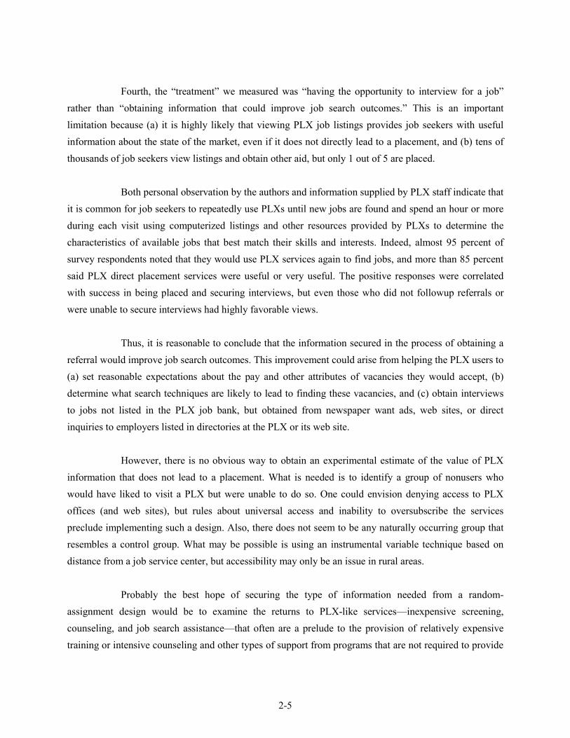
2-5
Fourth, the “treatment” we measured was “having the opportunity to interview for a job”rather than “obtaining information that could improve job search outcomes.” This is an importantlimitation because (a) it is highly likely that viewing PLX job listings provides job seekers with usefulinformation about the state of the market, even if it does not directly lead to a placement, and (b) tens ofthousands of job seekers view listings and obtain other aid, but only 1 out of 5 are placed.
Both personal observation by the authors and information supplied by PLX staff indicate thatit is common for job seekers to repeatedly use PLXs until new jobs are found and spend an hour or moreduring each visit using computerized listings and other resources provided by PLXs to determine thecharacteristics of available jobs that best match their skills and interests. Indeed, almost 95 percent ofsurvey respondents noted that they would use PLX services again to find jobs, and more than 85 percentsaid PLX direct placement services were useful or very useful. The positive responses were correlatedwith success in being placed and securing interviews, but even those who did not followup referrals orwere unable to secure interviews had highly favorable views.
Thus, it is reasonable to conclude that the information secured in the process of obtaining areferral would improve job search outcomes. This improvement could arise from helping the PLX users to(a) set reasonable expectations about the pay and other attributes of vacancies they would accept, (b)determine what search techniques are likely to lead to finding these vacancies, and (c) obtain interviewsto jobs not listed in the PLX job bank, but obtained from newspaper want ads, web sites, or directinquiries to employers listed in directories at the PLX or its web site.
However, there is no obvious way to obtain an experimental estimate of the value of PLXinformation that does not lead to a placement. What is needed is to identify a group of nonusers whowould have liked to visit a PLX but were unable to do so. One could envision denying access to PLXoffices (and web sites), but rules about universal access and inability to oversubscribe the servicespreclude implementing such a design. Also, there does not seem to be any naturally occurring group thatresembles a control group. What may be possible is using an instrumental variable technique based ondistance from a job service center, but accessibility may only be an issue in rural areas.
Probably the best hope of securing the type of information needed from a random-assignment design would be to examine the returns to PLX-like services—inexpensive screening,counseling, and job search assistance—that often are a prelude to the provision of relatively expensivetraining or intensive counseling and other types of support from programs that are not required to provide

2-6
universal access. Unfortunately for our work, studies of these employment and training programs focus onmeasuring the return from expensive treatments while ignoring the potential benefits from their PLX-likeservices.
A noteworthy example of how studies that use random-assignment designs ignore the valueof PLX-like services is the $23 million National JTPA Title II study (Bloom et al., 1993). In that study, acontrol group was created through random assignment after eligible volunteers received the screeningneeded to assign them to appropriate treatments. Focusing on the benefits of appropriate high-costtreatments is important. But had randomization occurred not only at the time job seekers were assigned totreatments, but also at application time, we would have obtained highly useful information about thevalue of low-cost treatments and the nature of selection bias.3 Similarly, random-assignment studies oftreatments given to UI claimants also might have provided useful information about the value of PLX-likeservices and the nature of selection bias had they used a two-stage randomization procedure.
Our objective is not to criticize other evaluations, but to point out that natural experimentsand random-assignment designs cannot be used to accurately measure the value of the informationprovided to job seekers by viewing listings and obtaining counseling from staff that does not necessarilylead to placement. Thus, the next best alternative would be to obtain information for similar servicesdelivered by programs that can use random-assignment designs. Given that such information is notavailable, our only alternative is to use the best possible nonexperimental techniques to provide a range ofplausible estimates. This analysis is presented in Section 2.2.
2.1.1 Summary of Key Findings from the Mail Survey
1. About one-third (34.4 percent) of job seekers referred by PLXs tried but failed toobtain an interview. Information from PLX staff suggests that most of theseindividuals applied too late to obtain interviews because jobs (or interview slots) werealready filled. While additional evidence is needed to remove individuals who werescreened out by employers or failed to obtain interviews for other reasons, thisevidence is sufficient to conclude that it should be possible in the future to identify alarge group of job seekers that closely resemble a control group derived from arandom-assignment design.
3 It is possible that excluding prescreening effects leads to substantial underestimation of the value of JTPA Title II program benefits. The returns
to classroom vocational training vary enormously depending on selection of curricula and whether the trainee excels in school. Therefore,helping potential participants to intelligently decide between taking the best available job and entering a training program could have largepositive effects on the returns to Title II spending (and large benefits to the potential clients).
2-7
2. About one-third (28.1 percent) of job seekers referred by PLXs did not try to secureinterviews. This group should be excluded from the comparisons designed to assessthe value of a placement because these individuals had no chance to be placed as aresult of the referral.
3. About one-fifth (22.2 percent) of job seekers referred by PLXs were not given joboffers, rejected job offers, or did not show up for work after accepting offers.Estimates of the job search outcomes of these individuals can be subtracted from theoutcomes of all job seekers who tried but failed to obtain interviews. The resultingmeasure describes what would have happened to those who were placed if they hadbeen unable to secure interviews. It is the difference between that measure and whatactually happened to those placed that most accurately measures the value of aplacement. Also, this difference can serve as benchmark for assessing the bias incomparing the outcome of placements to the outcome of referrals that do not lead toplacements.
4. About 50 percent of job seekers referred by PLXs had little, if any, employment in theyear prior to obtaining referrals. Measuring the effect of placements for this groupwith administrative data, but without the survey information, is extremely difficultbecause it is impossible to determine how long those referred were searching for workbefore and after receiving the referral.
5. Analysis of our survey data indicates that being placed reduces the unemploymentduration of job seekers with considerable work experience in our sample, most ofwhom are UI claimants, by about 7.2 weeks, and that of job seekers with little workexperience in our sample by about 3.8 weeks (relative to viewing listings, obtaining areferral, but not being placed).
6. That the measured effect of being placed was almost twice as great for individualswith substantial work experience than for those with little work experience isconsistent with the view that job seekers with substantial experience (a) will search forlong periods until they locate jobs that are well matched to their skills and interests,and (b) can afford to prolong the search because they receive UI benefits, have moresavings, and have other financial resources on which to draw.
7. At this point we do not know how close the estimates presented in point 5 come to thetrue effects for the universe of placed job seekers. The primary problem is that oursurvey sample was small and the response rate across different job seekers was notuniform. Also, some job seekers in the comparison group may have been deniedinterviews because employers felt that their credentials were not as good as thosealready interviewed. Nevertheless, we feel that the results are sufficiently accurate toproduce a first-approximation of the overall value of placements.
8. Using the estimates in point 5, which only imperfectly reflect the average reduction inunemployment duration, estimates of post-unemployment earnings fromadministrative data, and published statistics on the number of placements we estimatethat the total increase in earnings due to placements was about $45 million in 1998.This represents about 1.7 times the total cost of running the Washington State PLXs inthat year.

2-8
9. We feel that the highly respectable benefit cost ratio of 1.7 is a reasonable ball-parkfigure because we omit from the benefit calculations the value of information obtainedfrom viewing listings and interacting with staff that did not lead to a direct placement.Experimental evidence on job search assistance, which we believe is less potent thanPLX aid, suggests that those services reduce unemployment by about 1 week. Even ifreferral effect were this small, the total effect would be large because 4 out of 5referred PLX users are not placed. We also omit from the calculation the crowding outeffect of PLX aid, which negatively affects other job seekers. However, our estimatessuggest that the reductions in benefits due to crowding out are considerably smallerthan the increases in benefits had we included the value of referrals not leading toplacements.
10. Comparing the results in point 5 to those derived from use of nonexperimentaltechniques with the same dataset suggest that the nonexperimental techniquessubstantially underestimate placement effects. Unfortunately, the sample was not largeenough to directly test the specific model used in Chapters 4 and 5. Such a test wouldbe of great value, and would be possible if we assembled a larger database.
11. Information about why referrals did not lead to placement and the duration of jobsearch before and after referral were very useful. However, the other detailedinformation did not substantially improve our estimates over those we obtained withadministrative data alone.4
Our key conclusion is that use of a mail survey with telephone followup has the potential toprovide highly accurate estimates of the effect of having the opportunity to interview for a job as a resultof a PLX referral for all types of job seekers. We see no alternative but to use this method, at least untilsufficient information is obtained to create benchmark results that can validate nonexperimentalestimators. However, a survey cannot identify job seekers who resemble the control group needed toestimate the value of obtaining information from PLXs that do not lead to direct placements.
Surveys also can provide the information needed to improve measures of unemploymentduration using administrative data alone. This information is especially important for usingnonexperimental techniques to measure the effect of placements for nonclaimants.
4 The additional mail survey data may not have affected our results because for every person in our sample placed at a job, we selected one
person referred to the same job. This prematching may have greatly reduced the variation in our sample. In the near future, we will determinethe effect of the prematching. This was not possible in this study because we lacked time to assemble the followup administrative informationto make the relevant comparisons.
2-9
2.2 Measures Based on Administrative Data Alone
We used the 1998 mail survey to benchmark nonexperimental estimates of the value ofbeing placed relative to being referred but not placed using very large samples of administrative datacovering the job search of UI claimants. The administrative data and nonexperimental techniques werealso used to measure the value of obtaining the information that leads to referrals relative to not obtainingreferrals and usually not obtaining any PLX help. Our administrative databases included 328,815 separatespells of unemployment from 1987 through 1995 in Washington State, and 138,280 separate spells in1995 in Oregon.
The nonexperimental results use administrative data to hold constant differences in keycharacteristics of claimants who were (a) placed at jobs to which the were referred by PLXs, (b) referredto jobs but not placed at those jobs, and (c) who did not obtain referrals (and mostly did not use any PLXservices). The data permit us to hold constant demographic characteristics, prior work histories, UIbenefit entitlements, and most important, unemployment duration. These results are restricted to UIclaimants for the simple reason that the key variables used to measure job search outcomes and controlfor factors associated with PLX use are only available in the administrative data we used for claimants.
We make two different comparisons in the administrative data studies. We estimate theplacement effect by comparing the job search outcomes of placed claimants to the outcomes of claimantswho are referred but not placed, and we estimate the referral effect by comparing the job search outcomesof referred but not placed claimants to the outcomes of nonreferred claimants. The nonexperimentalplacement measures are quite similar to the results used to make the same comparisons with the mailsurvey. If anything, it appears that the nonexperimental results slightly underestimate the true effect.However, we would be more confident about this conclusion if the mail survey covered 1995, a yearcovered by both the Washington and Oregon administrative studies, and if the mail survey were largerand we were certain that it represented all claimants.
Unfortunately, we have no evidence from a random-assignment design or natural experimentto validate our estimates of referral effects, which represent the value of information obtained in thecourse of being referred. Thus, we have no means to determine precisely how much of the positive effectwe observed represents measurement bias. However, we have several pieces of information that suggestthe effects are positive First, experimental evidence on the effect of other forms of job search assistancesuggests that those treatments decrease unemployment duration by about 1 week. The key issue is

2-10
whether use of PLX job banks is likely to be more potent than the treatments studied using randomassignment designs. We suspect that PLX treatments are more potent because most of the studies examinethe effect of workshops that last only a few days. In contrast, most claimants who are referred but notplaced persist in using PLXs over a long period, usually until they find a job by some other means, andspend hours looking at job orders and obtaining other information on each visit. Second, the fact thatsurvey respondents who were not placed told us that they were highly satisfied with PLX services andthat they would use those services again bolsters the view that those services are valuable.
Third, regression adjusting the duration of unemployment for those who are referred but notplaced, initially substantially reduces the duration relative to the unadjusted mean. This reduction isstrong evidence that those who are referred but not placed have characteristics associated with longer thanaverage unemployment durations. Because selection bias usually leads to underestimation of programeffects, the regression adjusting appears to substantially reduce that bias, but probably does not eliminateit entirely.
Perhaps of even greater importance, regression adjusting makes less and less difference asthe duration of unemployment lengthens. This suggests that those referred but not placed and those notreferred become more and more similar to each other as time passes. This is highly relevant evidencebecause the primary test that a random-assignment design is properly implemented is to show that thedifference between simple means and regression adjusted means of the outcome variables are zero.
It also is worth noting that regression adjusting the duration of unemployment for thoseplaced substantially increases the duration of unemployment relative to the unadjusted mean. Thisincrease suggests that those placed have characteristics associated with shorter average durations ofunemployment. That the adjustments are far larger than those for job seekers referred but not placed, butuse the same set of control variables, suggest that more bias is present in the placement estimates, and thatthe regressions effectively remove much of that bias. However, we cannot be certain that this is the case.That the regression adjusted results resemble the results derived from the survey supports the view thatmuch of the bias is eliminated, but is not definitive. To obtain more definitive results we need to obtainunbiased estimates from a natural experiment using a representative sample.
Despite having considerable evidence that referral effects are positive and some evidencesuggesting that the nonexperimental techniques we used probably underestimate the true effect, we feelthat the positive effects are so large relative to those derived from random-assignment studies of similar

2-11
treatments that they cannot be considered definitive. We, therefore, present three estimates of the totalbenefits of direct placement services. The first uses the placement effect alone. The second adds half thereferral effect to the placement effect, and the third adds all of the referral effect to the placement effect.
Because it is most unlikely that all of the observed referral effect is due to measurement bias,we are highly confident that the true effect is considerably greater than the placement effect alone. It ishard to believe that obtaining information from a PLX makes job seekers worse off. This is particularly sowhen according to our mail survey 92 percent of those referred but not placed would use PLX job banksand other services to look for jobs in the future, 36 percent claimed that the information they obtained washighly valuable, and another 34 percent reported that the information was valuable.
2.2.1 Summary of the Washington Results
Use of the exceptionally large Washington State administrative database for 1987-1995provided highly positive assessments of the benefits of both referrals and placements. Overall, our mostimportant conclusions are that:
1. On average, placements reduce the duration of unemployment by 7.7 weeks relative tobeing referred but not placed. This nonexperimental estimate of the per-incident effectof placements relative to obtaining referrals are similar to those generated from use ofa survey. While several steps should be taken to increase our confidence that theseresults reflect those from a natural experiment, we feel that the bias in these results issmall enough for the similarity to support the view that the nonexperimental estimatesare reasonably close to the true values.
2. We produced plausible nonexperimental estimates of the per-incident effect ofobtaining information in the course of being referred relative to not being referred,and usually not obtaining any PLX help, appear plausible even though we have noexperimental evidence to serve as a benchmark. On average, our procedures produceestimates that referrals reduce the duration of unemployment by 2.1 weeks relative tonot being referred. Even if measurement error accounts for half of this figure, thecontribution to total benefits is large.
3. Estimates of the total benefits hinge on multiplying the per-incident effect times thenumber of incidents and average weekly post-unemployment earnings.
a. The administrative data provided accurate estimates of the incidence of beingplaced and being referred once the state employment security agency decided touse these data for in-depth analysis. On average, PLXs refer about 25,000claimants per year, of whom about 7,000 are placed.
2-12
b. Our procedure for estimating post-unemployment earnings is reasonablyaccurate, but could be greatly improved by applying techniques used with theseadministrative data in estimating the earnings losses due to job loss. Post-unemployment earnings of claimants average about $260 per week.
4. Estimates of the year-by-year variation in the pre-incident effect of placements andreferrals as well as the total benefits derived from direct placement services are muchin keeping with expectations. Total benefits are between 30 and 40 percent greater inthe trough of a business cycle than near its peak.
a. About one-third of the peak-to-trough reductions are due to reductions in theper-incident effect of placements and referrals as economic conditions improve.Placements, in particular, are more potent when good jobs are more difficult tofind and extended benefit programs considerably lengthen the period overwhich UI can be collected.
b. About two-thirds of the reductions are due to there being fewer claimants intotal during prosperous periods.
5. The cost of running the entire PLX system in Washington is easily derived frombudget figures. Those costs average about $25 million per year and vary very littlefrom year to year. Sixty percent of the funds come from the Federal Wagner-Peyserallocation, 15 percent from Federal Veterans funding, and the bulk of the remainderfrom state funds earmarked to assist claimants. It is not nearly as easy to determinehow much of the total goes to providing direct placement services, nor how much ofthose funds goes to aiding claimants. We use a ball park estimate of 35 percent for theportion spent on direct placement services going to claimants included in the benefitcalculations.
6. We produce the following three different benefit-cost estimates:
a. The lowest estimate assumes that the value of the information obtained ingetting referrals is zero. Thus, this measure only includes the value ofplacements relative to being referred but not placed. This produces a benefit-cost ratio of 1.2 (using the 35 percent estimate of the portion of costs going todirect placement services and including 1987-89, and 1995 years for which theincidence of placements and referrals is substantially underestimated).
b. A less conservative estimate assumes that half of the measured referral effect isdue to measurement error. This assumption produces a benefit-cost ratio of 1.9.
c. The least conservative estimate accepts the referral effect measure as beingaccurate. This assumption produces a benefit-cost ratio of 2.8.
Because the per-incident cost of placements and referrals is very low, we feelthat even the least conservative estimate is plausible. Key reasons for this vieware that: (1) receipt of UI payments greatly restricts the types of jobs claimantsare likely to accept before exhausting benefits; (2) some claimants would havegreat difficulty finding suitable work on their own after they have been jobless

2-13
for several months; and (3) we included 1987-89 and 1995 years for which theincidence of placements and referrals is substantially underestimated. Thus, wethink it is likely that placements and referrals will be particularly potent forclaimants.
The trend in unemployment reductions stemming from placements and referralsobtained after successively longer periods of being unemployed stronglysupports the view that, as unemployment duration lengthens, claimants havemore and more difficulty finding jobs on their own. The per-incident effectsjust about double from between the 9th and 19th week of unemployment spells.
7. Separate estimates suggest that UI payment reductions equal about 22 percent of thegain in earnings. Payment reductions are lower because weekly payments are aboutone-half of weekly earnings and because payments end after about 30 weeks, onaverage. Thus, except during periods covered by extended benefits, reductions in UIpayments are modest relative to the cost of providing direct placement services toclaimants. Nevertheless, employers benefit both from the reduction in UI payments,which usually will reduce their UI tax burden, and from claimants’ increased earnings.By lowering the cost of job loss, placement services reduce “the risk premium”workers would require to take jobs that are likely to end with permanent layoffs.
2.2.2 Summary of the Oregon Results
Like the Washington study, the Oregon study used an exceptionally large claimant databasedrawn from administrative records, and almost the same estimation techniques. However, there wereimportant differences between the Oregon and Washington studies. First, the Oregon database coveredonly 1 year, 1995. Second, the data had not been previously used for a similar research project. Third, wedid not conduct a mail survey in Oregon. Fourth, all the data processing was done by the OregonEmployment Department.
Our biggest problem stemmed from the fact that the data had not previously been used forsimilar research. Thus, we were able to determine that the Oregon person-level database did not cover allclaimants and all services those claimants received, but we were unable to determine why that was thecase. The problems we encountered were identical to those we had to overcome in working with similardata from Washington and other states. Thus, we are confident that eventually they can be overcome.Also of substantial importance, we learned a great deal about how to assist state employment securityagencies to assemble, process, and use these highly valuable data on their own.

2-14
We used the Oregon database to obtain critical evidence about the per-incident effect ofreferrals and placements. Those results were derived from a model almost identical to the one used inWashington. However, we had to use published statistics about the number of referrals and placements toestimates of the total effect.
Measured referral and placement effects were smaller both per incident and in total inOregon than in Washington in 1995. Our measure of being referred but not placed relative to not beingreferred indicates a reduction of unemployment by 1.1 weeks in Oregon compared to 1.6 weeks inWashington. Our measure of being placed versus being referred but not placed indicates a reduction of4.6 weeks in Oregon, compared to 6.6 weeks in Washington.
However, major differences in the procedures used to provide services and monitor jobsearch in Oregon versus Washington may explain why the results differed between these two states. Inparticular, Oregon spent more funds on assisting claimants than did Washington, and focused many ofthese activities in the first 10 weeks of each claimant’s unemployment spell. Unfortunately, this focusmay have substantially reduced the average effect because the per-incident effect is considerably higherafter the tenth week in Oregon. Also, the difference in effects between Oregon and Washington isparticularly great after the tenth week.
Perhaps of even greater importance, Oregon’s procedures for calling in claimants to obtainreferrals and have their job search plans reviewed may have led some Oregon claimants to search forwork more effectively, even if they did not obtain referrals, and others to stop collecting benefits (becomenonclaimants) if they were unable or unwilling to assiduously search for work. Thus, a major limitation ofthe Oregon analysis could be not including the effect of all types of services. This shortcoming can beovercome, but it probably would require use of an experimental design or analysis of the effect of Oregonprocedures on the incidence of benefit collection.
Using only the per-incident placement effects cited above together with published statisticson the number of claimants placed produced total benefits of $15.4 million in Oregon, compared to $19.8million in Washington. Moreover, we estimated that both states spent about the same amount on theirPLXs in 1995; however, Oregon spent about 38 percent of the total PLX budget to aid claimants,compared to Washington’s 25 percent. Thus the lower-bound benefit-cost ratio is 1.56 in Oregon,compared to 2.13 in Washington.
2-15
The least conservative estimate of total benefits in Oregon is $30.3 million versus $42.5million in Washington for 1995. These estimates include referral effects that capture the value ofinformation obtained in the course of being referred. The benefit-cost ratio is 3.06 in Oregon and 4.50 inWashington. Thus, in both states the least conservative estimate suggests that direct placement servicesreceived by claimants more than covered the entire cost of running the PLXs in each state in 1995.
Research presented in Chapter 6, however, suggests that crowding-out effects that adverselyinfluence nonreferred claimants reduce the benefits-cost ratios by about 20 percent. On the other hand, theleast conservative results omit the benefits from PLX services other than referrals and placements. Thevalue of these services could be large, particularly in Oregon.
2.3 Concluding Remarks
The main focus of this chapter was to provide a nontechnical discussion of the estimationproblems that must be overcome to produce accurate results. We, therefore, focused on how experimentaland nonexperimental techniques can be used to reduce self-selection and other forms of measurementbias. We then summarized our key findings and some of the estimation problems encountered inproducing the results for each of the three separate studies that measured per-incident referral andplacement effects and related benefits to costs.
The first study used a Washington mail survey to produce estimates of placement effects forall types of PLX clients. These results are reasonably close to those that would be derived from using anatural experiment where placed job seekers were compared to job seekers who requested referral to thesame jobs, but were unable to secure interviews because the jobs or interview slots were already filled.Importantly, while we do not consider our results to be definitive, we detail several steps that would likelyeliminate shortcomings in the data that would allow us to produce definitive estimates.
The second study used Washington administrative data to estimate referral and placementeffects for claimants alone. The nonexperimental estimation technique used produced placement effectestimates that were similar to those derived from use of the mail survey in the first study and theregression adjustments substantially reduced the effect relative to unadjusted means. We feel that thisevidence, taken together, suggests that our estimates are close to the true effect, but improving the surveydatabases is necessary for us to judge more precisely how much bias remains.

2-16
Unfortunately, we could not produce any referral estimates based on any type of random-assignment design or natural experiment to use as a benchmark for assessing bias in our nonexperimentalreferral effect estimates. The best we could do is compare our results to those from random assignmentdesigns applied to other types of job search assistance provided to claimants and other experiencedworkers. We recognize that our referral effects estimates are considerably larger than those derived fromexperimental studies. However, we feel that it is plausible that the support provided by PLXs issufficiently longer lasting and more potent to account for the effect being larger. Also, we believe thatresidual selection bias is likely to cause our techniques to underestimate referral effects. Nevertheless,while we produce total benefit estimates based on assuming our estimates are unbiased, biases lead tooverestimation equal to half the estimates, and all of the positive effect is due to measurement bias.
The third study used Oregon administrative data to examine referral and placement effectsfor claimants alone. That study produced results suggesting the effects were not quite as large as inWashington. However, other evidence suggests the effects are smaller mainly because Oregon requiresclaimants to participate in activities that increase incentives for claimants to search hard and effectively orstop collecting benefits.
The next three chapters present the technical details of the three studies that estimate per-incident effects. Chapter 6 presents the technical details of our estimate of crowding out effects. Chapter 7presents an overall summary of our findings and policy-oriented conclusions that is meant to beunderstandable to individuals with little interest in the technical details.

Chapter 3

3-1
3. DETAILS OF OUR RESEARCH USING THE WASHINGTON STATE MAIL SURVEY
Up to this point our goal was to make clear in a general way what we did and why we did itby providing sufficient information about public labor exchanges (PLXs), the context for this study, themeasurement problems, our results, and our conclusions. In this chapter, we provide the details of ouranalysis so that technical experts can independently judge the value of our work and others can gain amuch deeper understanding of precisely what we did and what we found.
3.1 Design of the Survey
The primary purpose of the survey was to produce estimates of the value of placements thatclosely resemble those that would be derived from a random-assignment design. Those results could thenbe used to assess the accuracy of estimates derived from administrative data alone and develop ways toimprove their accuracy.
In this chapter we use a natural experiment to produce separate estimates for claimants andother job seekers with a great deal of prior work experience and for job seekers with little prior workexperience. We do this to complement results presented in Chapter 4 that use administrative data toexamine PLX effects for claimants alone.
We also test the usefulness of data obtained from the mail survey that was not available inthe administrative files but strongly affected decisions to obtain PLX services and job search to improvethe accuracy of the nonexperimental estimates.
In our previous work, presented in Chapter 4, we compared all those referred but not placedto all those placed. As a result, many of those referred but not placed were referred to jobs that requiredvery different skills and interests than those required by the jobs to which individuals were placed.Although the control variables derived from administrative data might adequately take these differencesinto account, we also test restricting the comparison group to job seekers referred to the same jobs towhich the targets were placed.

3-2
An important by-product of selecting those placed and referred to the same job orders wasthat we also were able to add a great deal of information to the person-level files about the jobs to whichsample members were referred. This information included whether the job was full time or part time, thehourly wage rate, the number of slots to be filled, the number of referrals requested, and the requiredexperience, education, and age.
Delays in obtaining wage data prevented us from fully assessing the effect on ournonexperimental results of restricting referrals to jobs to which others were placed and adding job orderdata to the person level files. Also, somewhat to our surprise, we could not identify any variables, otherthan those in administrative data, that substantially affected our nonexperimental results. Thus, in oursubsequent discussion we primarily focus on what we learned from the unique information about whyreferred job seekers failed to be placed.
We also considered covering three groups of job seekers in the survey: (1) those placed as aresult of a PLX referral, (2) those referred but not placed, and (3) those not referred. Comparisonsbetween group 1 and group 2 could provide an estimate of the value of being placed, given that a jobseeker reviewed PLX job listings and obtained other information. Comparisons between group 2 andgroup 3 could provide an estimate of the value of obtaining information from a PLX that did not lead to adirect placement.
Ultimately, we decided to limit the survey to groups 1 and 2 because we recognized that thisis the only comparison where we might be able to mimic results from a random-assignment(experimental) design. The natural experiment we could study was based on identifying referred jobseekers who wanted to obtain a job interview but were denied the opportunity because the jobs werealready filled. However, we could not identify a natural experiment that could isolate individuals whowanted to obtain information from PLXs but were denied that opportunity.
Additional factors affecting our decision to limit the sample were that (a) except for UIclaimants, we had no way to obtain contact information for job seekers who did not visit PLXs and(b) much larger samples would be needed to produce statistically meaningful referral effect measuresbecause those effects were likely to be small.
Another key design issue was whether to use telephone followup with a mail survey. Thisdecision rested on whether the added information was worth the relatively high cost of using telephone

3-3
followup. We knew that it would probably cost about $30 per completed interview with telephonefollowup, but that a mail survey could be sent out at about one-tenth that cost. Also, we were fairly surethat the response rate would be low from a mail survey, but we did not know precisely how low theresponse rate would be. Perhaps most importantly, we were uncertain about how useful the informationwould be that we obtained from the survey.
Because we were uncertain about both the value of the information we would collect andhow low the mail response rate would be, we felt that it would be prudent to conduct a low-cost pilotstudy without telephone followup. We, therefore, decided that a sample of 3,000 placed job seekers and3,000 referred but not placed job seekers would provide sufficient information from a mail survey at areasonable cost. We thought that even if we got a very low response rate we would get returns from atleast 500 placed job seekers and 500 referred but not placed job seekers. This sample would be sufficientto evaluate the methods we used.
We then developed a mail survey instrument to meet our goals by obtaining detailedinformation from referred job seekers about:
1. The reasons referrals did not lead to placement;
2. The duration of job search before and after securing a referral;
3. The methods used to search for work and how successful these methods were;
4. Recent employment history and prospects for being recalled or holding on to currentjobs; and
5. Services received from the PLX other than referrals, such as participation in jobsearch workshops and use of resource rooms.
The survey instrument is presented in Appendix A.

3-4
3.2 Implementation of the Design
To implement our design we:
1. Identified job orders to which there was at least one placement and one referral notleading to placement during the first 7 months of 1998.
2. Identified the subset of job orders where there was at least:
a. One placement that was the most recent placement made to a job-seeker; and
b. One referral that either was the most recent referral or the only referral madewithin 4 weeks.
Steps 2a and 2b improved the chances that respondents would have clear memories of theseevents and that contact information would be correct. A second important attribute of our procedures isthat those selected because they were not placed as a result of a specific referral could not be placedwithin the subsequent 4 weeks as a result of another referral. If we did not take this step, we might haveseriously underestimated placement effects.
Selecting the most recent placement had almost no effect because it was rare for a person tobe placed more than once. Selecting the most recent referrals may have had some effect on the results.The sample was slightly altered because about 15 percent of those referred but not placed in one 4-weekperiod would be placed subsequently and a true experimental design would have prevented thoseindividuals from obtaining interviews. In the future, we could use a telephone survey to obtaininformation about the sequence of referrals that could determine the effect of alternative selectionprocedures. However, obtaining this type of information was not feasible in a mail survey.
It turned out that there were many job orders to which PLX users were referred, but no userswere placed and some cases where users were placed, but no one referred was not placed. Overall, only19 percent of all job orders received by Washington PLXs from January to July 1998 included at least oneplacement and at least one person referred to that job who was neither placed at that job nor referred toany other job listing within 4 weeks. However, those job orders accounted about 46 percent of all referralsand 29 percent of all placements.
We then selected a sufficient number of job orders to obtain a sample of 3,000 placementsand 3,000 individuals referred but not placed. If for a given job order only one person was placed or one

3-5
person was referred but not placed, we selected one person from each group. If there were three or moreplaced people and three or more referred but not placed people, we selected three people from each group.Otherwise, we selected two people from each group. We also oversampled job orders with multiplereferrals and placements to facilitate the determination of how the value of placements differed with thecharacteristics of the job orders.
Our survey sample included only 7 percent of job orders, but those orders included justunder 25 percent of all referrals and just over 15 percent of all placements.
3.3 Improving the Mail Response Rate
We expected a low response rate because job seekers referred by the PLX often had littleprior work experience and were looking for relatively low-wage jobs that sometimes were temporary orpart time. We, therefore, tested fancy packaging, cash incentives, and multiple mailings to improve theresponse rate at modest cost. One reason for conducting these tests is that we felt that states would beencouraged to employ these methods if we could find a low-cost way to obtain a response rate in theneighborhood of 50 percent.
Table 3-1 describes the response rates to our mailing. Part A of the table shows the resultsfrom the initial mailings, which tested three packages:
1. A “plain” mailing, which included a $1 bill and black and white survey, costing about$1.50 each;
2. A “fancy” mailing with postage stamps (not metered mail), multicolored instruments,inclusion of a special pen, and a $1 bill, all of which cost about $2.75 each; and
3. A mailing with added “money”—inclusion of a $5 bill instead of a $1 bill in the“plain” mailings, which cost about $5.50 each.
Column 2 shows that, compared to use of the plain package, the response rate from the fancypackage was somewhat higher, and that the response rate from the added money package wasconsiderably higher. However, the response rate was only 13.1 percent overall or 18.2 percent afteradjusting for undelivered mailings.

3-6
The second mailing brought the unadjusted response rate up to 19.2 percent. As anticipated,the response rate and mail return rates were much lower from the second mailing than the first. Clearly,those most likely to respond already had done so before the second mailing was made.
Table 3-1. Mail Response Rates and Cost for Four Different Designs
Numbermailed
Responserate
Returnedforwarding
address:
Adjustedresponse
rateUnitcost
Totalcost
Cost perresponse
No Yes1 2 3 4 5 6 7 8
A. First Mailing
1. Plain 2,500 11.1% 14.4% 17.3% 15.5% $1.50 $3,750 $13.49
2. Fancy 3,000 14.0% 14.4% 14.2% 19.5% $2.75 $8,250 $19.64
3. Added Money 500 17.2% 5.2% 2.8% 24.0% $5.50 $2,750 $31.98
4. Total 6,000 13.1% 13.7% 14.5% 18.2% $2.46 $14,750 $18.81
B. Second & ThirdMailing
5. Lottery 4,396 8.3% 5.2% 10.1% 9.9% $1.50 $6,594 $17.97
C. All Mailings 6,000 19.2% 17.5% -- 23.2% $2.05 $21,344 $18.54
Number ofresponses
1,151
Notes:1. In Section A the adjusted mail response rate (col 5) = responses (col 2) / [1 - average return rate (line 4)]. The actual return rate was not used
because it was artificially lowered by inclusion of $5 cash in the “added money” mailing.
2. The third mailing was to 141 of those for whom we had forwarding addresses from the second mailing. We received 20 responses. (The thirdmailing was limited by the materials we had on hand.)
The bottom line of column 8 shows that the overall cost-per-complete was $18.54. This isrelatively high for a mail survey because the response rate was low. Indeed, we suspect that the cost-per-complete from a telephone survey would not have been much higher because the response rate wouldhave been above 75 percent. Even with a response rate of 50 percent, the cost-per-complete of a telephonesurvey would have been about $30.
Column 8 also shows that, although the response rate was higher with the added packaging andcash, the additional responses did not cover the additional cost. Thus, if the only goal was to obtain “n”
3-7
responses, the plain package would be most cost effective. However, if the goal is to increase therepresentativeness of the responses, the added cost probably was justified.
An additional major problem with the package that included a $5 bill is that it reduced the mailreturn rate, which was 31.7 percent with the plain package, to a mere 8.0 percent. Further, only 2.8 percentof the packages with $5 bills were returned with forwarding addresses compared to 17.3 percent of the plainpackages. This largely precluded us from reaching individuals who were sent $5 bills, moved, and left amailing address.
3.4 Differences between Responders and Nonresponders
Overall, we obtained 1,115 usable responses from the 6,000 PLX-referred people to whomsurveys were mailed. Fortunately, there were more than enough respondents to reach our primaryobjective of determining the value of the survey data. This is the case even if the respondent sample is notparticularly representative either of all referrals or referrals to job orders where there was at least oneplacement and one referral not leading to a placement.
Nevertheless, understanding what characteristics made the survey recipients more or lesslikely to respond can provide information that should be kept in mind when analyzing the surveyresponses and help determine the best way to collect survey information from those referred by PLXs inthe future.
Table 3-2 displays the results of an ordinary least squares regression using the dummyvariable “responded-to-the-survey” as the dependent variable. Only variables that were statisticallysignificant at least at the 15 percent level were included. Table 3-2 also includes for each value its mean,standard deviation, and the coefficient times 10 percent of the variable mean. This last measure showshow a 10 percent change in the variable would affect the response rate. The variables are presented inorder by the size of this effect, with those with greatest effect presented at the top of the list.

3-8
Table 3-2. Regression on the Mail Response Rate
Variable nameRegressionCoefficient Mean
StandardDeviation
coef x.1 x mean
1. Placed 0.0829** 0.512 0.50 0.00422. Race: white 0.0552** 0.743 0.44 0.00413. Age in years 0.0021** 35.03 11.1 0.00234. Gender: female 0.0586** 0.382 0.49 0.00225. “Plain” initial mailing of mail survey -0.0359** 0.421 0.49 -0.00156. Months of experience asked for on job
order0.0013** 7.082 11.2 0.0015
7. Job order requires less than high schooleducation
-0.0633** 0.228 0.42 -0.0014
8. Highest earning quarter in 1997 0.0000* 2775 3402 0.00149. Referred in the first quarter of 1998 -0.0272** 0.490 0.50 -0.0013
10. Job seeker must be available to work 40 ormore hours
0.0191 0.676 0.47 0.0013
11. Job seeker lives in the eastern part of WA 0.0316** 0.347 0.48 0.001112. Job order Missing educational requirement -0.0285 0.347 0.48 -0.001013. Age 26-40 years -0.0199+ 0.467 0.50 -0.000914. Job seeker must be willing to relocate for
job-0.0298* 0.260 0.44 -0.0008
15. Hourly wage missing in highest earningsquarter of 1997
0.0251* 0.298 0.46 0.0007
16. Job seeker lives in Seattle -0.0297* 0.212 0.41 -0.000617. Agricultural industry classification from
SIC-0.0638** 0.090 0.29 -0.0006
18. Minimum acceptable wage less than $6.60 0.0245 0.137 0.34 0.000319. Applicant must be greater than 18 years old
on job order-0.0474* 0.059 0.24 -0.0003
20. Handicapped or disabled program 0.0705* 0.031 0.17 0.000221. Job seeker attending school 0.0425 0.037 0.19 0.000222. College education required on job order 0.0727 0.013 0.12 0.000123. Minimum acceptable wage greater than
$13.200.1121+ 0.008 0.09 0.0001
24. Years of experience missing from job order -0.3700+ 0.001 0.03 0.0000Note: ** indicates coefficient is significant at the .01 level.
* indicates coefficient is significant at the .05 level.
+ indicates coefficient is significant at the .10 level.
3-9
The variable with the largest effect is whether the person was placed as a result of a referral.The survey sample included equal numbers of individuals placed and individuals referred but not placed.These results suggest that individuals who regarded the referral as a “significant” event were more likelyto respond. We suspect that this is because they could more easily remember those events, and possiblybecause they wanted to show their appreciation for the services they received. This view is reinforced bythe strong positive effect of being referred to full-time job on the probability of responding.
Demographic and work-history factors also are of considerable importance. Whites are muchmore likely to respond than people of other races; women are more likely to respond than men; olderindividuals are more likely to respond than younger individuals; and individuals with more education aremore likely to respond than those with less education. Also, even holding constant demographiccharacteristics, individuals with high earnings are more likely to respond than those with low earnings,and those applying to jobs that require more experience are more likely to respond than those applying forjobs requiring less experience.
These results are consistent with the responses to a broad range of government-sponsoredsurveys indicating that individuals who are more likely to trust the government are more likely to respondand that individuals with an educational background that makes responding to a pencil and paper surveyeasy are more likely to respond.
Finally, the statistical analysis confirms that individuals were less likely to respond to theplain packages than to either the fancy packages or the packages containing $5 bills. Also, individualswho were asked about events that occurred further in the past were less likely to respond.
3.5 Design of the Analysis
Our primary goal was to determine the difference in job search outcomes between whathappened to those who received PLX referrals (and other information), which is directly observable, andwhat would have happened to those same people had this aid not been obtained, which is not directlyobservable. Researchers agree that the best means to determine what would have otherwise happened is tocreate a control group by denying services (at least for a short period) to a randomly selected group ofindividuals requesting services. Comparisons between targets, who volunteer to receive a service, andcontrols, who volunteer but are denied the service, produce unbiased results because all the factors

3-10
influencing post-service outcomes except service receipt itself are distributed identically between thetargets and controls.
In contrast, other measurement approaches require use of statistical techniques to take intoaccount differences between the comparison group and target group in factors influencing both thedecision to obtain a service and job search outcomes. Because many of these factors are very difficult tomeasure, there is always some doubt about whether the results are unbiased.
Unfortunately, it is not feasible to use a random-assignment design for estimating the effectof PLX services. First, the program requires universal access. Second, even if services could be denied, itwould require major modifications to the way PLXs currently operate to effectively deny access.Ordinarily, PLX services are exceedingly easy to obtain from office visits, visits to public sites such aslibraries that have computers containing the PLX listing, and even from home computers through theInternet.
Nevertheless, it is worth describing the steps involved in obtaining a placement from a PLXreferral to determine (a) what would be learned from alternative random-assignment designs, and (b)whether there are naturally occurring groups that resemble those that would be created by a random-assignment design.
Table 3-3 (which also was presented in the Executive Summary) breaks the process ofobtaining a placement in Washington State into 10 steps. If we were going to set up a random assignmentexperiment to measure the value of PLX direct placement services, our top priority would be to create acontrol group by randomly preventing some job seekers at Step 2 from reaching Step 3. In other words,we would deny job seekers who have decided that they want to use PLX services the opportunity to do so.
This could be done in practice if PLXs were run like a health club and required an ID card togain access to PLX offices and entry into PLX computers. Essentially, we would randomly tell peoplewho wanted to join the club that no more applications were being taken.

3-11
Table 3-3. Job Search Path from Deciding to Search for Work Through Deciding to Use PLXs toPlacement by a PLX
Steps to surmount Path ending outcomes
Step 1. Unemployed worker decided to search for work
a. Recalled by former employerb. Retiredc. Dropped out of labor force
Step 2. Job seeker decided to use PLX No desire to use PLX
Step 3. Job seeker gained access to PLX Unable to use PLX because services wereunavailable or too difficult to access
Step 4. Looked at PLX listings Found no suitable jobs
Step 5. Found promising listings Decided not to interview for those jobs
Step 6. Tried to obtain an interview a. Job or interview slots filled
b. Employer rejected job seeker based on
prescreening
Step 7. Obtained interview Did not receive an offer
Step 8. Received an offer Rejected offer
Step 9. Accepted offer Did not show up for work
Step 10. Showed up for work Placed by PLX system
We would then compare the outcomes of those who used PLX services to those who wantedto use the services but were denied the opportunity to do so. In this case, the treatment is “obtaininginformation about the job market.” In some cases this treatment leads to direct placements and in othercases leads to acquiring information that improves decisions about (a) the types of jobs to search for, (b)when to accept job offers, and (c) how to search for those jobs.
Thus, all job seekers who visit PLXs would be potential beneficiaries. Even those who donot find any suitable jobs in PLX listings could benefit because not seeing a suitable job would indicate tothese job seekers that finding a suitable job may be difficult and it might be reasonable to lower theirexpectations. Thus, randomization at any other point could lead to underestimation of the value of PLXservices.
Randomization at the point job seekers decide to use PLXs is likely to be particularlyvaluable because (a) job seekers who choose not to use PLXs are likely to have different employment

3-12
prospects from those who choose to use PLX services, and (b) obtaining detailed data that could identifythose differences is likely to be particularly difficult. Indeed, it appears that the evidence suggesting PLXservices are of little value suffers from not adequately taking into account PLX use being triggered bylack of access to better sources of information or having exhausted those sources.
In addition to obtaining a benefit estimate for the respondent sample as a whole, it would behighly desirable to determine how benefits differ for those who are referred but not placed versus thosewho are referred and placed. Having this information could greatly improve PLX operations.
If, for example, the net benefit of placements is more valuable than providing informationthat does not lead to placements, then more effort should go to tasks that lead to placements, such asworking with firms to obtain listings. However, if the reverse is true, more effort should go to helping jobseekers use the information to locate jobs on their own. Moreover, the relative merits of information andplacements could vary across job seekers with different characteristics.
Also, knowing more about the value of different elements of the help provided by PLXscould strongly affect how we measure the returns to PLX services. In particular, if we knew that almostall of the benefits of the PLX accrue to those directly placed, we could focus on measuring the value ofplacements by using administrative data to compare job search outcomes of those placed to those referredbut not placed.
Even if we could use a random-assignment design, it is unclear whether we could devise away to separately measure the value of the information in cases where the job seeker is, and is not,directly placed. Part of the problem stems from placement being an outcome, not a treatment. However,we could ask employers to randomly reject candidates to whom they otherwise would offer jobs at Step 8.But it is dubious that doing this would give us the information we need because the rejection would likelyaffect the job search of those rejected, and thereby, distort the results.
A more viable alternative is to randomize after the job seeker has obtained information froma PLX, obtained a suitable referral, and decided to follow up that referral by arranging an interview. Forexample, we could ask employers to tell job seekers assigned to the control group that they have filled allinterview slots at Step 6 (whether or not this is the case). The results of randomization at this point would

3-13
allow us to measure the value of interviewing for a job, given a suitable referral is found.1 We could thensubtract this value from the net benefit to all PLX users to get an estimate of the value of viewing joblistings and getting related information, but not getting an interview.
Rather than use experimental evidence, we also could compare the outcomes of individualswho were placed following receipt of a job offer to individuals who rejected job offers or did not show upfor work after accepting an offer, holding constant observable characteristics. However, there is a stronglikelihood that those who rejected an offer would have superior outcomes because they were takingpreferable jobs they found on their own, and this information might not be readily observable.
Of enormous importance, the mail survey can provide the information we need to identify anaturally occurring group of job seekers who resemble a control group derived from randomization at thepoint they try to set up an interview after receipt of referral contact information. The naturally occurringgroup is not identical to a control group because (a) group members could subsequently obtain interviewsfrom PLX-supplied contact information, and (b) some members would have been rejected by employers.
However, the positive value of the subsequent interview might offset the distorting effect ofnot being able to secure interviews at all, and PLX officials at all levels concur that, with rare exceptions,PLX screening is sufficient for employers to want to interview referred job seekers. Officials believe thatlags inherent in removing listings easily can result in large numbers of job seekers obtaining referrals toolate to secure interviews. Thus, unless the jobs are filled, the vast majority of referred job seekers whorequest interviews can secure interviews.
By identifying referred job seekers who reach each Step from 4 through 10, the mail surveycan also provide the information needed to determine the bias in using administrative data to compare thejob search outcomes of those placed to those who would have been placed had they tried to obtain aninterview. In estimating the bias, we make the simplifying assumption that only those placed wereaffected by interviewing. If this was the case, we could use information about the number and outcomesof job seekers who were interviewed but not placed (and therefore reached Step 7 but not Step 10) toestimate what would have happened to those stopping at step 6a had they secured interviews but not been 1 As would be the case in being rejected for a job, being told interviews were unavailable also could affect subsequent job search. For example,
job seekers might wrongly assume suitable jobs are scarcer than they previously believed. Such distortions limit the value of a random-assignment design when the information itself is valuable. Even when expensive, long-lasting treatments are being offered, it is possible toprovide information that affects the behavior of control group members. For example, in the National JTPA Title II evaluation, screening themembers of the control group to the point they are willing to volunteer for a training program could increase the likelihood they would seek outthis treatment through other sources.

3-14
placed. Subtracting out the outcomes of those interviewed but not placed from the comparison groupoutcomes allows us to estimate the effect of being placed relative to individuals who would have beenplaced had they secured interviews.
In reality, information obtained during the interviews could affect the distributions andoutcomes of all those interviewed. Because this effect cannot be distinguished from the effect of beingplaced, the simplifying assumption makes it easier to calculate the effects and discuss the results. Also,because it likely that the effect of having the information from an interview is small relative to the effectof being placed, the assumption produces results that are close to being exactly correct anyway.
Of greatest importance, the net benefit estimates are not affected in any way because wemultiply what probably is a slight overestimate of the effect on those placed times the number placed. Thealternative would be to multiply an accurate estimate of the interview effect by the total numberinterviewed.
Thus, even though we cannot use a random-assignment design, we focus on using the mailsurvey to learn as much as we can about (a) the returns to interviewing for a job based on a PLX referraland (b) biases in using administrative data to measure the value of placements, given the PLX user isreferred.
3.6 Estimators Used in the Analysis
Estimator 1a is the primary estimator of interest. It measures the difference between thoseinterviewed and those who tried but failed to obtain an interview. The estimator produces results similarto those from a random-assignment design to the extent (a) those who tried to secure an interview wereunable to do so because the jobs were filled or no more interviews could be scheduled, and (b) those whotried to secure an interview to one job listing, did not try, or were unable to secure interviews to other job-openings.
(1a) Interview Effect = W(intv) - W(ntintv)where:
W(j) = weeks from referral to job is found for group jfor j equal to:
intv = interviewed as a result of a referral (reached Step 7)ntintv = not interviewed, but tried to obtain an interview (stopped at Step 6)

3-15
In comparisons designed to measure the bias in estimates derived from use of administrativedata alone to measures that more closely resemble those from a random-assignment design we use thefollowing two estimators.
Estimator 1b is used with mail survey data. It is derived by multiplying estimator 1a by theinverse of the proportion of job seekers who were interviewed who are placed. This estimator is based onthe assumption that only placed individuals benefit from information obtained in the interviews. Analternative way of looking at the assumption is that for job seekers who are not placed, the effect ofreceiving the treatment, which in this case is obtaining an interview relative to trying but failing to obtainan interview, is zero.
(1b) Placement Effect-1 = INTV/PLC x [W(intv) - W(ntintv)]where:
INTV = total number interviewedPLC = number placedW(j) = weeks from referral to job is found for group jfor j equal to:
intv = interviewed as a result of a referralntintv = not-interviewed, but tried to obtain an interview
Estimator 2 is used with administrative data that identify placements and referrals but do notidentify why job seekers were not placed.
(2) Placement Effect-2 = W(plc) - W(ref)where:
W(j) = weeks from referral to job is found for group jfor j equal to:
plc = placed (reached Step 10)ref = referred, but not placed (reached Step 5, but not Step 10)
Because estimator 1b produces results similar to those from a random-assignment design, wewill use the difference between estimator 1b and estimator 2 as an indicator of the bias in estimator 2.Before looking at the empirical evidence, we can get an idea of how the two estimators differconceptually by breaking each down into its constituent parts based on the following six referraloutcomes:
1. PLACED Were placed at the job to which they interviewed. (Reached Step 10);
2. NO-SHOW Did not show up for work, after accepting an offer. (Stopped at Step 9);

3-16
3. NO-ACCEPT Did not accept a job offer, after receiving an offer. (Stopped at Step 8);
4. NO-OFFER Did not obtain a job offer, after an interview. (Stopped at Step 7);
5. NO-INTERVIEW Tried, but failed, to obtain an interview. (Stopped at Step 6); and
6. NO-TRY Did not try to obtain an interview. (Stopped at Step 5).
Figure 3-1 shows how the six outcome groups fall into the target and comparison groupsinherent in each of the two estimators.
Estimator 1 Estimator 2
1. PLACED } target-22. NO-SHOW target-13. NO-ACCEPT (INTV)4. NO-OFFER comparison5. NO-INTERVIEW } quasi-control (REF)6. NO-TRY - -
Figure 3-1. How referral-outcome groups are organized to produce Estimators 1 & 2
Estimator 1 is based on the ratio of the number placed (group 1) to the number interviewedbut not placed (groups 2, 3, and 4); and the difference in weeks unemployed among those interviewed(groups 1, 2, 3, and 4) and those who tried but failed to obtain an interview (group 5). Estimator 2 isbased on the difference in weeks unemployed among those placed (group 1) versus those referred but notplaced (groups 2, 3, 4, 5, and 6).
The two estimators are identical if all job seekers referred by PLXs are either placed(group 1) or tried but failed to obtain an interview (group 5). The two estimators also are the same ifweeks unemployed is identical among all those who were not placed (groups 2, 3, 4, 5, and 6).
Conversely, the differences between the two estimators are greatest when: (1) large numbersof individuals are in groups 2, 3, 4, and 6, (2) weeks unemployed among members of groups 2, 3, 4, and 6are similar to each other; and (3) weeks unemployed among members of groups 2, 3, 4, and 6 are verydifferent from weeks unemployed among members of group 5.
However, the difference between the two estimators could be small even if large numbers ofjob seekers are in groups 2, 3, 4, and 6, and their weeks unemployed differ sharply from those for
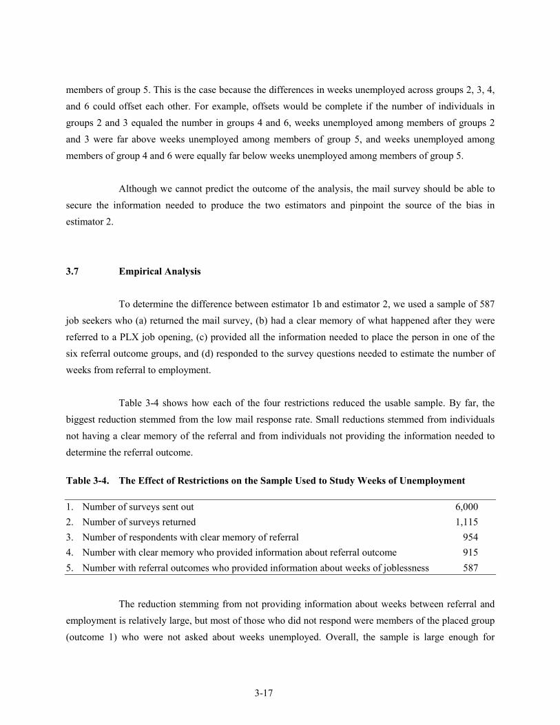
3-17
members of group 5. This is the case because the differences in weeks unemployed across groups 2, 3, 4,and 6 could offset each other. For example, offsets would be complete if the number of individuals ingroups 2 and 3 equaled the number in groups 4 and 6, weeks unemployed among members of groups 2and 3 were far above weeks unemployed among members of group 5, and weeks unemployed amongmembers of group 4 and 6 were equally far below weeks unemployed among members of group 5.
Although we cannot predict the outcome of the analysis, the mail survey should be able tosecure the information needed to produce the two estimators and pinpoint the source of the bias inestimator 2.
3.7 Empirical Analysis
To determine the difference between estimator 1b and estimator 2, we used a sample of 587job seekers who (a) returned the mail survey, (b) had a clear memory of what happened after they werereferred to a PLX job opening, (c) provided all the information needed to place the person in one of thesix referral outcome groups, and (d) responded to the survey questions needed to estimate the number ofweeks from referral to employment.
Table 3-4 shows how each of the four restrictions reduced the usable sample. By far, thebiggest reduction stemmed from the low mail response rate. Small reductions stemmed from individualsnot having a clear memory of the referral and from individuals not providing the information needed todetermine the referral outcome.
Table 3-4. The Effect of Restrictions on the Sample Used to Study Weeks of Unemployment
1. Number of surveys sent out 6,0002. Number of surveys returned 1,1153. Number of respondents with clear memory of referral 9544. Number with clear memory who provided information about referral outcome 9155. Number with referral outcomes who provided information about weeks of joblessness 587
The reduction stemming from not providing information about weeks between referral andemployment is relatively large, but most of those who did not respond were members of the placed group(outcome 1) who were not asked about weeks unemployed. Overall, the sample is large enough for

3-18
assessing the difference between the two estimators, and the low response rate does not affect the internalvalidity of this test.
Column 1 of Table 3-5 shows how the 587-person sample is distributed across the sixoutcome groups. Over 56 percent of the sample were placed (group 1). This number is high because weoversampled those placed, and those placed had a higher response rate than those referred but not placed.Column 2 shows the distribution in the underlying population had we not oversampled those placed. Onlyabout 15 percent of those referred were placed at the jobs to which they were referred.2
Table 3-5. Distribution of the Sample and PLX Referred Job Seekers by Referral Outcome
Full Natural Distributionsample distribution if interviewed
(1) (2) (3)1. Placed at the job to which they interviewed. 56.2% 15.0% 40.0%2. Did not show up for work, after accepting an offer. 2.4% 4.6% 12.4%3. Did not accept a job offer, after receiving an offer. 2.9% 5.6% 15.0%4. Did not obtain a job offer, after an interview. 6.3% 12.2% 32.6%5. Tried but failed to obtain an interview. 17.7% 34.4%6. Did not try to obtain an interview. 14.5% 28.1%
100.0% 100.0% 100.0%
Note: The full sample includes roughly four times more placed individuals than the natural distribution because the mail survey was stratified toinclude equal numbers of those placed and those referred but not placed.
The most interesting (and important) information in column 2 is that 34.4 percent of theindividuals referred to a given job opening tried but failed to obtain an interview. This means that thereare plenty of individuals in the quasi-control group needed to produce estimator 1. Also, of considerableinterest is that 28.1 percent of individuals obtaining referral information did not even try to obtaininterviews.
In addition, column 2 shows that 12.2 percent of the sample failed to receive an offerfollowing an interview. But almost as many job seekers, 10.2 percent, turned down offers or failed toreport to work after accepting an offer.
2 The 15 percent placement figure applies to the one referral that was used to select the sample. Since most job seekers are referred to several
openings the probability of placement after using the PLX is much greater than 15 percent. For members of our sample, it probably is around 30percent.

3-19
Finally, column 3 shows that the probability of being placed given the job seeker obtained aninterview is quite high, 40 percent, and that the probability of having the opportunity to take the job is avery respectable 67 percent (40+12.4+15.0).
To our knowledge, this is the only information available about the reasons PLX users fail tobe placed at jobs to which they were referred. Being unable to secure interviews is an important factoraccounting for 40 percent of the failures. As noted earlier, as far as we can determine almost all of thefailures to set up interviews are due to either the jobs already being filled or no more interview slots beingavailable at the point the job seeker contacts the employer. Not receiving a job offer is relatively rare,accounting for only 14 percent of the failures. The remaining 46 percent of failures are due to factorsunder the job seekers’ control, such as not attempting to set up interviews, rejecting offers, and notshowing up for work after accepting offers.
As noted in Section 3.7, there would be no difference between estimator 1b and estimator 2,if all referred job seekers were either placed or failed to obtain an interview. That just under 50 percent ofthose referred are in these two categories suggests that there is plenty of opportunity for estimates basedon comparisons of those placed to those referred but not placed to be biased.
Column 1 of Table 3-6 shows the mean value for weeks of unemployment (following receiptof a referral). This variable is the actual reported weeks of unemployment for those who had found jobswhen surveyed. For those who had not found jobs, we assumed that they would be unemployed for 18weeks. This is a conservative estimate because it is only slightly longer than the actual average elapsedtime between when individuals received referrals and when they returned their surveys.
A key reason for using 18 weeks for those who had not found new jobs is that about one-halfthe sample had very little work experience in the year before obtaining the referral. Thus, it is likely thatmany of the individuals who did not find work within 18 weeks stopped looking. In contrast, we used amuch longer maximum jobless duration in our earlier work restricted to UI claimants because: (a) manyclaimants would not take jobs paying little more than their UI benefits until those benefits were exhaustedafter 26 or more weeks, (b) claimants had a much stronger attachment to the labor force, and (c) mostclaimants unemployed for many weeks were searching for work in a period where jobs were much moredifficult to find than in 1998.
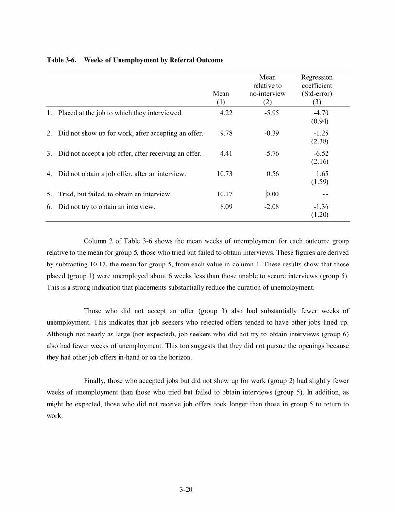
3-20
Table 3-6. Weeks of Unemployment by Referral Outcome
Mean Regressionrelative to coefficient
Mean no-interview (Std-error)(1) (2) (3)
1. Placed at the job to which they interviewed. 4.22 -5.95 -4.70(0.94)
2. Did not show up for work, after accepting an offer. 9.78 -0.39 -1.25(2.38)
3. Did not accept a job offer, after receiving an offer. 4.41 -5.76 -6.52(2.16)
4. Did not obtain a job offer, after an interview. 10.73 0.56 1.65(1.59)
5. Tried, but failed, to obtain an interview. 10.17 0.00 - -
6. Did not try to obtain an interview. 8.09 -2.08 -1.36(1.20)
Column 2 of Table 3-6 shows the mean weeks of unemployment for each outcome grouprelative to the mean for group 5, those who tried but failed to obtain interviews. These figures are derivedby subtracting 10.17, the mean for group 5, from each value in column 1. These results show that thoseplaced (group 1) were unemployed about 6 weeks less than those unable to secure interviews (group 5).This is a strong indication that placements substantially reduce the duration of unemployment.
Those who did not accept an offer (group 3) also had substantially fewer weeks ofunemployment. This indicates that job seekers who rejected offers tended to have other jobs lined up.Although not nearly as large (nor expected), job seekers who did not try to obtain interviews (group 6)also had fewer weeks of unemployment. This too suggests that they did not pursue the openings becausethey had other job offers in-hand or on the horizon.
Finally, those who accepted jobs but did not show up for work (group 2) had slightly fewerweeks of unemployment than those who tried but failed to obtain interviews (group 5). In addition, asmight be expected, those who did not receive job offers took longer than those in group 5 to return towork.

3-21
Column 3 of Table 3-6 shows the regression adjusted differences in weeks of unemploymentrelative to those who tried, but failed to obtain interviews (group 5). These results are based onregressions that use 112 administrative variables and 59 survey variables. After considerableexperimentation, we decided to use all the variables that were available in the database, that reflect factorsobservable before the referral date. (Appendix B describes the regression equation and the variables inconsiderable detail.)
The regression-adjusted values are similar but not identical to the unadjusted mean valuesshown in column 2. Importantly, the regressions increased the duration of unemployment relative togroup 5 for individuals who (a) were placed (group 1) by 1.25 weeks, (b) did not receive offers (group 4)by 1.09 weeks, and (c) those who did not try to obtain interviews (group 6) by about 0.72 weeks. Theseresults indicate that members of these three groups had characteristics that made them more likely thanaverage to find work quickly.
In contrast, the regressions decreased the duration of unemployment for individuals who didnot show up for work (group 2) by 0.86 weeks, and did not accept offers (group 3) by 0.76 weeks. This isevidence that members of these two groups had characteristics associated with longer than averagedurations of unemployment.
The information in Tables 3-5 and 3-6 is sufficient to produce estimator 2, which comparesthe duration of unemployment of those placed (group 1) to those referred but not placed (groups 2, 3, 4, 5,and 6). As shown in section A of Table 3-7, the regression adjusted duration of unemployment for thoseplaced is -4.7 weeks (relative to those who did not secure interviews), and the value for those not placedis -0.7 weeks (based on summing the regression adjusted means times the proportion of individuals ineach of the remaining groups). Thus, estimator 2 indicates those placed were unemployed 4.0 less weeksthan those referred but not placed.
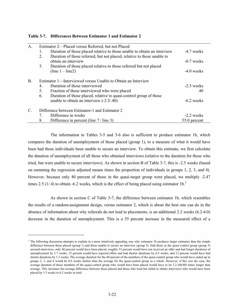
3-22
Table 3-7. Differences Between Estimator 1 and Estimator 2
A. Estimator 2—Placed versus Referred, but not Placed1. Duration of those placed relative to those unable to obtain an interview -4.7 weeks2. Duration of those referred, but not placed, relative to those unable to
obtain an interview -0.7 weeks3. Duration of those placed relative to those referred but not placed
(line 1 – line2) -4.0 weeks
B. Estimator 1—Interviewed versus Unable to Obtain an Interview4. Duration of those interviewed -2.5 weeks5. Fraction of those interviewed who were placed .406. Duration of those placed, relative to quasi-control group of those
unable to obtain an interview (-2.5/.40) -6.2 weeks
C. Difference between Estimator-1 and Estimator 27. Difference in weeks -2.2 weeks8. Difference in percent (line 7 / line 3) 55.0 percent
The information in Tables 3-5 and 3-6 also is sufficient to produce estimator 1b, whichcompares the duration of unemployment of those placed (group 1), to a measure of what it would havebeen had those individuals been unable to secure an interview. To obtain this estimate, we first calculatethe duration of unemployment of all those who obtained interviews (relative to the duration for those whotried, but were unable to secure interviews). As shown in section B of Table 3-7, this is -2.5 weeks (basedon summing the regression adjusted means times the proportion of individuals in groups 1, 2, 3, and 4).However, because only 40 percent of those in the quasi-target group were placed, we multiply -2.47times 2.5 (1/.4) to obtain -6.2 weeks, which is the effect of being placed using estimator 1b.3
As shown in section C of Table 3-7, the difference between estimator 1b, which resemblesthe results of a random-assignment design, versus estimator 2, which is about the best one can do in theabsence of information about why referrals do not lead to placements, is an additional 2.2 weeks (6.2-4.0)decrease in the duration of unemployment. This is a 55 percent increase in the measured effect of a
3 The following discussion attempts to explain in a more intuitively appealing way why estimator 1b produces larger estimates than the simple
difference between those placed (group 1) and those unable to secure an interview (group 5). Had those in the quasi-control group (group 5)secured interviews, only 40 percent would have been placed, roughly 33 percent would have not received an offer and had longer durations ofunemployment by 1.7 weeks, 15 percent would have rejected offers and had shorter durations by 6.5 weeks, and 12 percent would have hadshorter durations by 1.3 weeks. The average duration for the 60 percent of the members of the quasi-control group who would have ended up ingroups 2, 3, and 4 would be 0.6 weeks shorter than the average for the quasi-control group as a whole. However, if this was the case, theaverage duration of those members of the quasi-control group who would have been placed would have to be 1.2 (60/40) times longer thanaverage. This increases the average difference between those placed and those who tried but failed to obtain interviews who would have beenplaced by 1.5 weeks to 6.2 weeks in total.

3-23
placement and suggests that estimates that lack information about reason for not being placedsubstantially under-estimate true effects.
3.8 Placement Effects for Job Seekers with Strong and Spotty Work Records
The initial comparison of the two estimators provides useful insights into the bias in anestimator based on the difference between those placed versus those referred but not placed. Thus, it isworthwhile to use estimators 1b and 2 to: (1) assess the bias in our previous attempts to estimate the effectof placements on claimants, and (2) produce estimates of placement effects for groups that we did notstudy in our previous work.
We examined several different ways to divide the sample into a group that stronglyresembled UI claimants and a group that was very different from claimants. The division that made themost sense was to separately examine individuals with strong work records, whom we defined as havingthree of four quarters of employment in 1997, versus spotty work records, whom we defined as having 0,1, or 2 quarters of employment in 1997.
This split resulted in an almost equal number of job seekers being in each division. UIclaimants made up about 65 percent of the strong work record history group, but only about eight percentof the spotty work record group. The two groups sharply differed from each other, while within eachgroup members were quite similar. In particular, most members of the 3 or 4 quarter group had highearnings and earnings in all four quarters, while members of the 0, 1, or 2 quarter group had low earningsand earnings in zero or one quarter. Most importantly, the estimation procedures produced highly similarresults for all claimants and nonclaimants with 3 or 4 quarters of earnings, while results for individualswith 3 or 4 quarters were quite dissimilar from results for the 0, 1, or 2 quarter group.
Even before we obtained results for each group separately, we had evidence that results forthe two groups would differ—by far the best determinant of duration of unemployment (next to beingplaced) in our regressions were the number of quarters a person was employed in the year beforeobtaining a referral.
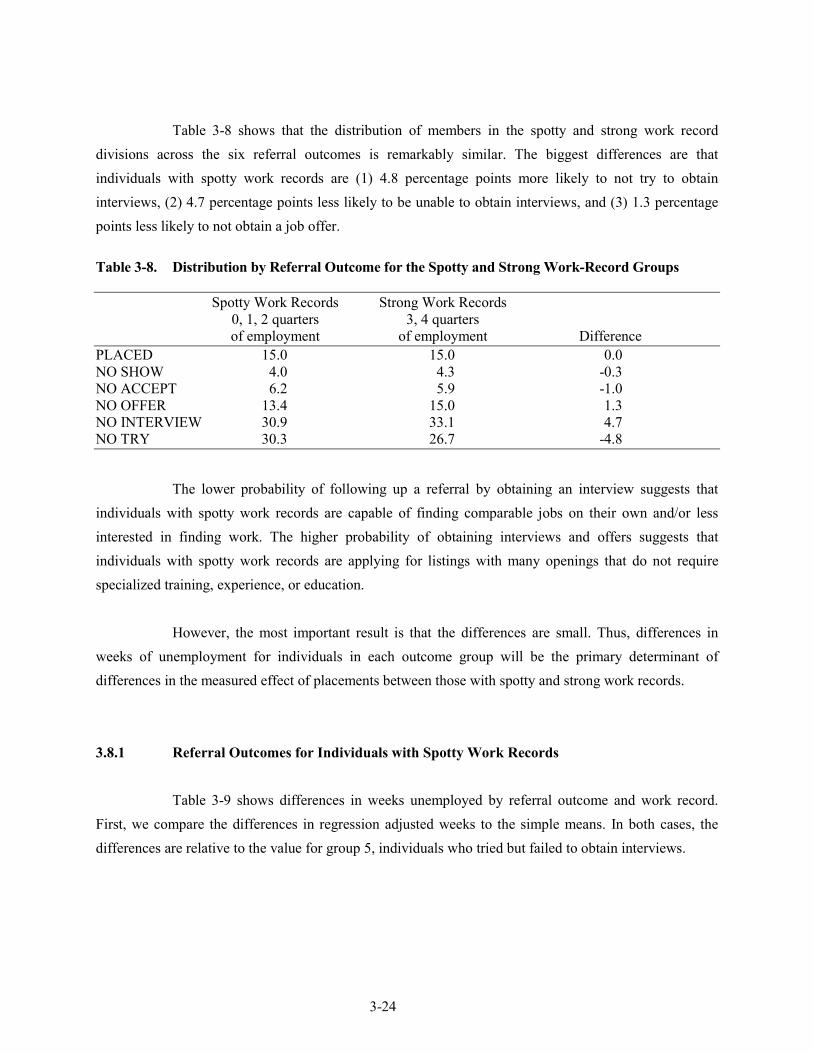
3-24
Table 3-8 shows that the distribution of members in the spotty and strong work recorddivisions across the six referral outcomes is remarkably similar. The biggest differences are thatindividuals with spotty work records are (1) 4.8 percentage points more likely to not try to obtaininterviews, (2) 4.7 percentage points less likely to be unable to obtain interviews, and (3) 1.3 percentagepoints less likely to not obtain a job offer.
Table 3-8. Distribution by Referral Outcome for the Spotty and Strong Work-Record Groups
Spotty Work Records Strong Work Records0, 1, 2 quarters 3, 4 quartersof employment of employment Difference
PLACED 15.0 15.0 0.0NO SHOW 4.0 4.3 -0.3NO ACCEPT 6.2 5.9 -1.0NO OFFER 13.4 15.0 1.3NO INTERVIEW 30.9 33.1 4.7NO TRY 30.3 26.7 -4.8
The lower probability of following up a referral by obtaining an interview suggests thatindividuals with spotty work records are capable of finding comparable jobs on their own and/or lessinterested in finding work. The higher probability of obtaining interviews and offers suggests thatindividuals with spotty work records are applying for listings with many openings that do not requirespecialized training, experience, or education.
However, the most important result is that the differences are small. Thus, differences inweeks of unemployment for individuals in each outcome group will be the primary determinant ofdifferences in the measured effect of placements between those with spotty and strong work records.
3.8.1 Referral Outcomes for Individuals with Spotty Work Records
Table 3-9 shows differences in weeks unemployed by referral outcome and work record.First, we compare the differences in regression adjusted weeks to the simple means. In both cases, thedifferences are relative to the value for group 5, individuals who tried but failed to obtain interviews.

3-25
Table 3-9. Reductions In Weeks Unemployed By Referral Outcome for Job Seekers With Strongand Spotty Work Records
Spotty0, 1, 2 quarters
Strong3, 4 quarters
Differencestrong versus spotty
reg mean diff reg mean dif regression mean(1) (2) (3) (4) (5) (6) (6) (8)
1. placed -4.10 -6.21 2.11 -4.22 -5.66 1.44 -0.12 0.54(2.03) (1.38)
2. no show -5.64 1.12 -6.76 -2.66 -1.99 -0.67 2.98 -3.11(4.49) (3.92)
3. no accept -2.97 -5.99 3.02 -7.35 -5.70 -1.65 -4.38 0.29(4.26) (3.41)
4. no offer 4.29 -0.94 5.23 0.44 2.30 -1.86 -3.85 3.24(3.43) (2.10)
5. no interview 0.00 0.00 0.00 0.00 0.00 0.00 0.00 0.00
6. no try -3.02 -0.61 -2.40 2.62 -3.52 6.15 5.64 -2.91(2.39) (1.82)
7. grp 2-4 0.20 -1.88 -2.08 -1.96 -0.39 1.55 -2.16 1.41
Natural Exp.8. est-1b -3.80 -9.02 -5.22 -7.17 -6.25 0.93 -3.37 2.76
9. grp 2-6 -1.03 -0.72 0.31 0.27 -1.17 -1.44 1.30 -0.45
Non-exper.10. est-2 -3.07 -5.49 -2.42 -4.50 -4.49 -0.01 -1.43 1.00
11. est-2 – 1b 0.73 3.53 2.80 2.67 1.76 -0.91 1.95 -1.76
NOTE: Standard errors are in parentheses.

3-26
Columns 1, 2, and 3 of Table 3-9 show that regression adjusted weeks unemployed forindividuals with spotty records diverge sharply from the unadjusted means. Group 2, no-shows, shift froma mean of 1.12 weeks of unemployment longer than group 5, no-interviews, to a point estimate of 5.64weeks less than no-interviews. In contrast, group 4, no-offers, shifts from a mean of .94 weeks less thanno-interviews to 4.29 weeks more.
That regressions produce a large decrease in weeks for no-shows indicates that this grouphas characteristics associated with difficulty finding work. Nevertheless, those individuals who are no-shows appear to have another job lined up. The large increase in weeks for no-offers indicates that thisgroup has characteristics associated with easily finding work. Thus, the no-offer group may have beenqualified for the jobs, but indicated that they were unenthusiastic about working for the given employer.
The remaining differences are smaller than for no-shows and no-offers. Those who did notaccept offers were unemployed 5.99 fewer weeks than no-interviews, but regression adjustment reducedthe difference to 2.97 weeks less. Although no-accepts have characteristics associated with a somewhatquicker return to work, the results suggest that not accepting an offer is due to knowing about a morepromising opportunity.
Lines 8 and 10 of Table 3-6 show placement measures based on estimators 1 and 2 usingmeans and regression adjusted weeks of unemployment. The measures on lines 7 and 9 show why thosemeasures diverge from the difference between those placed versus those who try but fail to obtaininterviews. Given the large differences in weeks unemployed based on means and regressions, we wouldexpect that the placement measures will differ greatly as well.
Line 8 shows estimator 1b, which is based on comparing the outcomes for those interviewedto those who tried but failed to obtain interviews and thus comes close to the results of a randomassignment design. Using the regression-adjusted weeks measures we found that estimator 1b shows thatplacements reduce unemployment by 3.80 weeks.
Estimator 1b results are only about 10 percent less than the 4.10 reduction in unemploymentshown on line 1, based on comparing those placed to those who tried but failed to obtain interviews. Thedifference is small because weeks unemployed for the three groups interviewed but not placed is only0.20 weeks longer than for those who tried but failed to obtain interviews.

3-27
Regression adjusting the results for the no-try group reduces the duration of unemploymentby 2.40 weeks to -3.02 weeks. This surprising result suggests that no-trys were not lazy, but knew ofbetter opportunities than afforded by the referrals. Finally, those placed were unemployed 6.21 fewerweeks than no-interviews, but regression adjustment reduced the difference by 2.11 weeks to 4.10 weeks.This result suggests that placed individuals are not a random draw of those referred, but have betterqualifications and higher motivation to return to work.
In contrast, when mean values are used, estimator 1b produces a much greater estimate ofthe decrease in unemployment of 9.02 weeks. The estimate is greater in part because the mean of thoseplaced is 6.21 weeks less than the mean for those who failed to obtain interviews. However, it also isgreater because the mean of those interviewed but not placed is -1.99 weeks, which suggests that thosewho would have been placed had they obtained interviews would have been less likely than average toobtain jobs by other means.
Line 10 of Table 3-9 shows that estimator 2, which is the difference between being placed(group-1) and being referred but not placed, (groups 2, 3, 4, 5, and 6), is about 20 percent less thanestimator 1 when based on regressions and 65 percent less when based on means. In both cases, thereductions are related to individuals in groups 2, 3, 4, and 6 being unemployed fewer weeks than those ingroup 5.
Overall, these results reinforce the view derived from looking at individuals with all workrecords together that estimator 2 tends to underestimate the true effects of placements by about 20percent. However, in contrast to results for all work record groups together, regression adjusting theresults makes a big difference. This, in turn, suggests that it is important to have large samples ofindividuals in each of the following three groups: (a) placed, (b) interviewed not placed, and (c) tried butfailed to obtain an interview.
3.8.2 Referral Outcomes for Individuals with Strong Work Records
The results shown in columns 4, 5, and 6 of Table 3-9 for workers with strong work recordsdiffer markedly from those for individuals with spotty records. For starters, the differences between theresults based on means versus regressions tend to be small and often are in the opposite direction from thedifferences for those with spotty work records.

3-28
Regression adjustment makes a very large difference only for individuals in group 6, no-try.That regression adjustment creates a 6.15 week increase in duration is evidence that those who do not tryto obtain interviews have characteristics associated with easily finding work, and as we might expect,suggests that those who do not try are simply less interested in returning to work.
Regression adjustment increases weeks unemployed by those placed by 1.44 weeks, whichas with the spotty record results, suggests that those placed have better qualifications for jobs that are indemand, and are more highly motivated to return to work than the average referred person.
Regression adjustment decreases the weeks of unemployment for members of all threegroups who are interviewed but not placed. This result suggests that these job seekers have characteristicsassociated with having difficulty finding work.
The finding that the regression adjustment tends to be in the opposite direction for those withstrong versus spotty work records suggests that the regression-based estimators will be larger than themean-based estimators. The finding that the regression adjustments tend to be smaller for those withstrong work records suggests the difference between the regression-based and mean-based estimators alsowill be small.
The results on lines 8 and 10 show that these expectations are realized. In particular, thedifferences in estimator 1b using regressions versus means are much smaller and in the opposite directionfor those with strong work records versus weak work records.
However, the most important result is that placements reduce unemployment by 2.67 moreweeks, a 60 percent increase, when measured using regressions with estimator 1b versus estimator 2. Theprimary reason for this difference is that, on average, individuals interviewed but not placed areunemployed 1.96 weeks fewer than individuals who were unable to obtain interviews.
Based on the assumptions underlying estimator 1b, had those unable to obtain interviews hadthe opportunity to interview, the 60 percent who would not have been placed would have beenunemployed 1.96 fewer weeks than the 40 percent who would have been placed. Thus, those who wouldhave been placed would have been unemployed 2.85 weeks more [1.96/(40/60)], in the absence ofplacement.

3-29
In contrast, as shown on line 9 of column 4, there is almost no difference between whathappened to those who were referred and not placed versus those who tried but failed to obtaininterviews. The differences among members of the five referred and not placed groups almost exactlybalance out. Thus, estimator 2 produces almost the same estimate of the placement effect as thecomparison between those placed and those who tried but failed to obtain an interview.
Thus, although the above argument may be hard to follow, the difference between estimator1b and estimator 2 is almost entirely due to the differences between what happened to those who obtainedinterviews but were not placed versus what happened to those who tried but failed to obtain an interview.
3.9 Summary of Reductions in Weeks-Unemployed Due to PLX Placements
In summary, Table 3-9 presents measures of weeks unemployed for:
Two types of job seekers, those with:
Spotty work records—0, 1, or 2 quarters of earnings in 1997, and
Strong work records— 3 or 4 quarters of earnings in 1997.
Using two estimators:
Estimator 1b—which compares placed individuals to individuals who would havebeen placed had they been able to obtain interviews;
Estimator 2—which compares placed individuals to individuals who were referred,but not placed.
With two measures of weeks unemployed:
A measure based on mean values; and
A regression adjusted measure.
It is our view that the results using estimator 1b based on regression adjusted weeksunemployed measures produces the most accurate results. Estimator 1b indicates that placements reducethe duration of unemployment by 7.17 and 3.80 weeks for job seekers with strong and spotty workrecords, respectively.

3-30
The large difference in placement effects between those with spotty and strong work recordsprimarily stems from job seekers with strong work records, who obtain interviews that do not lead toplacements, being unemployed 1.96 fewer weeks than the average job seeker unable to obtain aninterview. This suggests that those who were unable to obtain an interview, but otherwise would havebeen placed, would have been unemployed considerably longer than average. In contrast, job seekers withspotty work records who obtain interviews that do not lead to placements are only unemployed 0.20weeks longer than the average job seeker unable to obtain an interview.
Comparing the results using estimator 1b to those using estimator 2 suggests that measuresbased on the nonexperimental estimator 2, which compares all those referred but not placed, understatethe true effect of placements by about 50 percent for job seekers with strong work records and by about25 percent for job seekers with weak work records.
Regression adjusting weeks unemployed for job seekers with spotty work records makes anenormous difference when using estimator 1b. This is evidence that these job seekers are highlyheterogeneous and the observable differences have large effects on the duration of unemployment.Regression adjusting weeks unemployed for job seekers with spotty work records also makes a bigdifference when using estimator 2, but the difference is only about one-half as great as with estimator 1b.
In contrast, regression adjusting the results for job seekers with strong work records makesonly a small difference when estimator 1b is used, and virtually no difference when estimator 2 is used.These results suggest that these job seekers are highly homogeneous. One reason for the homogeneitycould be that we selected the comparison group of those referred but not placed from job seekers applyingto the same jobs to which the target group was placed.
It seems highly plausible that matching on job opening characteristics would have a farlarger effect on job seekers with strong work records, than those with spotty records. It is far more likelythat those with strong work records would confine their search to jobs similar to those that they have heldin the past and would readily accept suitable offers. Most job seekers with spotty work records probablyapply for jobs that require little training or experience. Thus, job seekers with spotty work records whohave very different backgrounds and motivations to work would apply to the same jobs.

3-31
Our overall conclusion is that estimator 1b produces highly credible results for individualswith strong work records. Our primary reasons for this conclusion are: (1) conceptually estimator 1bshould produce highly accurate estimates, (2) the results are similar to those obtained using much largersamples of UI claimants shown in Chapter 4, and (3) weeks unemployed estimated for each of the sixseparate referral-outcome groups (shown in column 4 of Table 3-9) are much in keeping withexpectations. In particular, job seekers rejecting offers or not showing up for jobs are likely to do sobecause they are able to find jobs more quickly that are at least as good as those to which they werereferred. Thus, it is reasonable that the adjustment inherent in estimator 1b suggests job seekers in thequasi-control group who would have been placed had they secured interviews would have beenunemployed considerably longer than those who would have found jobs on their own.
We also believe that estimator 1b produces highly credible results for individuals with spottywork records for similar reasons. In particular, it makes sense that individuals with spotty work recordswho are not given offers would have a lot of trouble finding work. Indeed, the 4.29 weeks longer than theno-offer group is unemployed is a major reason for estimator 1b results being smaller for job seekers withspotty work records than those with strong work records.
However, unlike the results for job seekers with strong work records, we have not previouslyexamined the effects of placements on job seekers with spotty work records. Our expectations were thatindividuals with spotty work records would need more help finding work than individuals with strongwork records. Therefore, the placement effects would be larger for those with spotty work records. Theevidence suggests otherwise.
On further reflection we think that job seekers with spotty work records have difficultyfinding high-wage jobs because of their lack of work experience and experience looking for jobs, but wesuspect that it is easy to locate the kinds of jobs these individuals usually take. In contrast, it is the jobseekers who have strong work records who will search until they find a job matching their skills andinterests. Therefore, public labor exchanges end up having a greater effect on the duration of joblessnessof job seekers with strong, rather than spotty work records.

3-32
3.10 Translating Weeks Unemployed to Total Benefits
The primary challenge in accurately assessing the benefits of PLX direct placement servicesis determining the per-person effect of those services. The reason this element is so difficult is that weneed to compare directly observable outcomes to outcomes that are not directly observable. So far, thisanalysis solely focused on obtaining these estimates and using them to examine the bias in alternativeestimators.
In contrast, once we determine the per person effect on weeks unemployed it is simple totranslate them into total effects measured in weeks. The number of people affected can be generated bothfrom the person-level files we used for our analysis, as well as from summary statistics maintained by thePLXs.
However, the ultimate goal of the research is to obtain benefit measures that can becompared to cost measures. To translate reductions in weeks unemployed to dollars of benefits, we needto know how those reductions affect earnings. In past work, we estimated earnings effects by assumingthe gain was equal to one-thirteenth of average quarterly earnings in the quarter following the return towork.
Line 1 of Table 3-10 presents an estimate of the total increase in earnings generated by eachplacement reducing the duration of joblessness of claimants and other job seekers with strong workrecords by 7.2 weeks and job seekers with spotty work records by 3.8 weeks. Line 2 shows that averageweekly earnings in the quarter following the return to work (for those whom we observed their earnings)was $260 for job seekers with strong work records and $180 for those with weak work records.Multiplying the number of weeks times the earnings per week produces a measure of the per-personincrease in earnings, which as shown on line 3, is $1,872 for job seekers with strong work records and$684 for those with weak work records.
Line 4 of Table 3-10 shows the number of placements made according to official statistics toclaimants and nonclaimants in 1998. If we make the conservative assumption that only claimants are inthe steady employment group, the total increase in earnings to those individuals is $20,861,568(11,144 x $1,872). The total increase in earnings to those with spotty work records is $23,965,992(35,038 x $684). For both groups together the total increase in earnings is $44,827,560, which is about 1.8times the cost of running the entire PLX system in 1998.

3-33
Table 3-10. Earnings Increases and the Benefit-Cost Ratio Stemming From Reductions in WeeksUnemployed
Steady(1)
Spotty(2)
Both
1. Reduction in weeks unemployed 7.2 3.8
2. Earnings per week $260 $180
3. Increase in earnings (line 1 x line 2) $1,872 $684
4. Number Placed in 1998 11,144 35,038
5. Total Increase in earning (line 3 x line 4) $20,861,568 $23,965,992 $44,827,560
6. Cost of running the PLXs in 1998 25,000,000
7. Benefit to Cost Ratio (line 5/line 6) 1.8
Because the basic estimates of the reduction in unemployment shown on line 1 are based ona relatively small and nonrepresentative sample we regard the above estimate as indicative of the trueeffect rather than definitive. However, it is clear that the estimates for the universe could be much smallerthan those shown on line 1 and the total effect would still be far greater than the cost.
A major drawback in making the above calculation is having to wait about 9 months fromwhen the survey is conducted to obtain the wage record data needed for this analysis. Because our newperson-level file contains information about hourly pay and hours of work for the job openings at whichindividuals were placed, we could produce an alternative measure and see how it compares to the onebased on quarterly earnings.
For job seekers with strong work records, we expect that both methods will produce similarresults. For job seekers with spotty work records, the results using the two measures may be substantiallydifferent. The difference could stem from job seekers with spotty work records only wanting to work forlimited periods. If this was the case, estimates of earnings gains based on quarterly earnings probablywould much better reflect increases in earnings.
Although far beyond the scope of this analysis, once we are confident that we can measurereductions in unemployment, it would be worthwhile to directly estimate earnings gains in the short andlong run. This is technically feasible for workers strongly attached to the labor force using powerful

3-34
estimators developed to examine the costs of worker displacement. However, these estimators should bemodified to take into account the large subsequent earnings gains, noted in previous research, stemmingfrom returning to work sooner. Also, several years need to elapse before long-term effects can beestimated.
Estimating the earnings gains for job seekers with spotty work records also is important todetermine if there is an adverse trade-off between quickly returning to work and subsequent long-termearnings growth. We do not anticipate that use of PLXs would produce an adverse trade-off because ourcrowding-out analysis suggests that most of the reduction in job search time stems from improving theinformation possessed by the searchers. Clearly, it would be useful to directly confirm this even ifmeasuring the earnings effects for job seekers with little prior work experience is difficult.
3.11 Summary and Conclusions
The primary achievement of this chapter is demonstrating that use of a mail survey withtelephone followup can provide unique information about the reasons referrals do not lead to placements,which permits identification of a group closely resembling a control group that would be generated from arandom-assignment design. Thus, the procedure tested here has great potential for providing accuratemeasures of the effect on the duration of job search of interviewing for jobs listed in PLX job banksfollowing reviewing job listings and obtaining other information.
Also of great importance, it should be possible to use the survey-based estimates to measurethe bias in estimators derived from administrative data alone. Thus, it should be highly feasible to developa low-cost system for accurately monitoring on-going operations, as long as PLXs can identify who isreferred to jobs listed with PLXs and who is placed as a result of those referrals.
In addition, this study suggests that measuring the effect of direct placement services on jobseekers with strong work records may be substantially improved by adding detailed data about the joborders to which these individuals are referred and by limiting comparisons between those placed to jobseekers referred to the same job-listings. Key evidence suggesting this is the case comes from the fact thatregression adjusting mean values does not make much difference. Indeed, the similarity between themeans and regressions suggest that the results strongly resemble those derived from a random-assignmentdesign.

3-35
In contrast, accurately measuring the effect of direct placement services on job seekers withspotty work records is likely to be much more difficult than for those with strong work records. First, theeffects appear to be much smaller, which means large samples will be required to ensure results arestatistically different from zero. Second, job seekers with spotty work records appear to be highlyheterogeneous, and those differences are hard to narrow using administrative data alone.
Evidence suggesting this is the case comes from the fact that regression adjusting meanvalues makes a large difference. However, at this time we cannot determine how much of the differencesare due to natural variation stemming from having small samples versus lacking precise information toidentify job seekers who tried to obtain interviews but were unable to do so because the jobs or interviewslots were already filled.
Clearly, future results could be greatly improved by obtaining data from a much larger, andfar more representative sample of PLX users, and by securing information to be sure that we identifyindividuals denied interviews because jobs were filled.
Ideally, the sample of job seekers with strong work records should include about 750individuals placed at jobs to which they were referred and 1,500 individuals referred but not placedindividuals. The sample of job seekers with spotty work records should include about 1,250 individualsplaced at jobs to which they were referred and 2,500 individuals referred but not placed.
Such a sample should be able to be secured through a mail survey with telephone followupat a cost of about $30 per complete or $180,000 for 6,000 completes. This is a substantial sum, butnowhere near the cost of using a pure random assignment.
There is no doubt that obtaining highly valuable survey information from a largerepresentative sample is feasible and would greatly reduce uncertainty about the true value of PLX directplacement services. At the same time, this study suggests that there would still be some uncertainty aboutthe value of placements as distinct from obtaining information that improves job search outcomes short ofinterviewing for jobs listed with PLXs. In particular, it is difficult to eliminate the conservative biasstemming from job seekers referred but not placed to one opening being placed subsequently.

3-36
However, this uncertainty is trivial compared to the uncertainty of not knowing the value ofinformation that improves job search outcomes short of leading to placement or job interviews. Becausefor each placed job seeker there are roughly five job seekers who obtain PLX information who are notplaced, even small positive effects of obtaining the information would have very large total benefits.
Unfortunately, we do not see how a survey could have an impact on this issue because it isnot obvious that there is any naturally occurring group that is denied the opportunity to use PLX services.One possibility worth pursuing with administrative data is determining if there is a systematic relationshipbetween PLX use and time required to get to local offices. If a measure of time to get to an officeappeared to affect usage, this measure could be used as an instrumental variable to estimate the effect ofPLX usage and not just the value after labor market information has been obtained.

Chapter 4

4-1
4. DETAILS OF OUR RESEARCH USING WASHINGTON STATE ADMINISTRATIVE DATA
In this chapter, we describe our analysis of an exceptionally large and detailed administrativedatabase covering the use of public labor exchange (PLX) direct placement services by UnemploymentInsurance (UI) claimants in Washington State from 1987 through mid-1995. For most years, the databaseis a 20 percent sample of the universe and, in total, includes 328,815 separate spells of unemployment. Aspell is a period of benefit collection during which there is no gap in payments of more than 3 weeks. Onaverage, each claimant has about 3.5 spells during the 8 1/2 years covered by the database.
The primary goal of this analysis is to measure the reductions in unemployment stemmingfrom claimants’ use of PLX direct placement services. We focus on UI claimants because theadministrative data provide a great deal of information about each claimant’s period of unemployment,work history, demographic characteristics, and the characteristics of his or her labor market. Thisinformation may be sufficient to greatly reduce, if not eliminate, selection and other forms of bias in ourmeasures.
In addition, detailed data are available for claimants who obtain PLX referrals as well as acomparison group of UI claimants who do not obtain referrals (and usually obtain no PLX services). Thispermits obtaining information about the value of PLX referrals (and other informational services) that donot lead to a direct placement—a placement at a job to which a PLX user was referred.
One key advantage of using claimant data is that the data provide a highly accurate view ofwhen claimants became unemployed, when they obtained PLX services, and, in most cases, when theyreturned to work. Controlling for the duration of unemployment at the point a referral is obtained is thesingle most important step to reducing selection bias. Indeed, much of the evidence suggesting PLXservices are ineffective are seriously flawed because they fail to take into account the fact that manyclaimants do not even begin to use PLXs until well after apparently similar claimants have alreadyreturned to work.
In contrast, it is close to impossible to use administrative data alone to determine when PLXusers who are not claimants first began to search for work and when they decided to give up searching forwork. The problem is most severe for job seekers who have spotty work records and, therefore, do notqualify for UI benefits. Because these workers spend a lot of time out of the labor force, periods of job

4-2
search and periods of joblessness do not coincide. Without accurate information about when individualsare searching for work, we would most likely overestimate the value of PLX services by comparing PLXusers who are searching for work to nonusers, many of whom are not searching.
A different problem exists for individuals with strong work records who are not UIclaimants. These individuals would qualify for UI benefits if they were unemployed, did not quit jobs,were not ill or otherwise unable to work, and actively searched for work. As a result, nonclaimants withstrong work records are often still employed during their job search. For this group, the pattern ofquarterly earnings tells us nothing about when search started, and since many employed searchersultimately stay with current employers, we often would not know when job search stopped. Studyingnonclaimants with strong work records who are not working faces us with a similar situation to that instudying individuals with spotty work records. We would be comparing PLX users, who are searching forwork, with nonusers, many of whom are unable to work or uninterested in finding work.
Another advantage of confining our analysis to claimants is that we can examine reductionsin UI expenditures as well as reductions in periods of job search. Reductions in UI trust fund expendituresare one of the most popular benefits of PLX services with legislators and business groups. Thisenthusiasm stems from savings in UI outlays being directly translated into reductions in a firm’s UI taxrate. These reductions occur because UI experience rating systems base a firm’s tax rate on the amount ofbenefits collected by workers the firm lays off. Thus, demonstrating high cost effectiveness with respectto saving UI payroll tax dollars would do a great deal to persuade key groups that labor exchange servicesare valuable to them.
Finally, this work is aimed at helping states develop a system to monitor ongoingperformance. At present, there is exceptionally strong interest in putting in place high-qualityperformance measures. Measures of trust fund savings and increases in short-term earnings are the twovalue-added measures that stand the best chance of being put in place because (a) it is highly feasible tocreate reasonably accurate, low-cost measures of these two factors, and (b) these measures are attractiveto a variety of groups.
Our interest in producing procedures for states to routinely employ has led us to useestimating techniques that can be applied using standard statistical packages and are reasonably easy tointerpret. In particular, we want to use the fewest number of separate comparisons and mainly rely onordinary least squares regressions. We have tested far more complicated alternatives, but have found that

4-3
the more esoteric estimators do not materially change the results. Rather, they primarily serve to make itvery difficult for nonexperts to interpret or replicate the results.
4.1 Design of the Analysis
Fundamentally, we want to answer the following two questions:
1. How many weeks sooner do directly placed claimants find jobs than would be thecase if they obtained referrals but were not placed?
2. How many weeks sooner do referred but not placed claimants find jobs than would bethe case if they did not use PLXs?
We strongly prefer addressing the above questions rather than simply determining how manyweeks sooner do all referred claimants find jobs than would be the case if they did not use PLXs? Asnoted on pages 3-11 and 3-12, the difference in the returns to providing information versus directlyplacing a person at a job has important implications for how PLXs should be organized and how theireffectiveness should be monitored. In particular, measurement problems would be much easier toovercome if the value of providing referrals and other information that helps PLX clients find jobs ontheir own was close to zero and, therefore, these effects could be omitted from total benefit estimates.
However, if, as appears to be the case, providing information that helps clients find jobs ontheir own is valuable, omitting those returns would substantially underestimate the total benefits, andcould lead decisionmakers to take actions that reduce total benefits. Also, of considerable importance,measures of the effect of referrals not leading to placements can provide information about the potentialbias in our estimators.
To answer question 2, we need to compare the duration of job search of claimants who arereferred from the point of referral to the point the job seeker returns to work, to the duration of job searchof a nonreferral claimant who is identical in every way to the referred person except having been referred.One way to make this comparison is to create a control group by using an experimental design—randomly denying access to PLX services to job seekers requesting aid. This is infeasible because PLXsare required to provide universal access. A second way is to find a naturally occurring group thatresembles a control group because it was unable to secure key services. This procedure was used in thepreceding chapter with the help of a mail survey, but cannot be done with administrative data alone.

4-4
A third way is to determine the effect of all pertinent factors on the duration of job searchand then use these estimates to predict the duration of job search for those placed and those referred butnot placed had those individuals not obtained PLX aid. The primary drawbacks of applying this techniqueare that (a) it is difficult to obtain all the variables needed to predict job search duration with absoluteaccuracy, and (b) without use of a random-assignment design or a natural experiment it is impossible toknow if the duration equation includes all the pertinent variables. Nevertheless, the technique used herecan substantially narrow the range of plausible answers. More specifically, we should be able to produce alower-bound estimate that still suggests PLX services are highly cost effective.
Table 4-1 illustrates the sources of potential measurement problems. The table shows thatamong claimants who change jobs, those who are referred but not placed are considerably less likely tohave returned to work by the end of the first full quarter of unemployment than those who are notreferred. However, by the third full quarter referred but not placed claimants are considerably more likelyto have returned to work than not referred claimants.
Table 4-1. The Probability of Returning to Work for Not Referred, Referred not Placed, andPlaced Job Changers
Duration ofunemployment Not referred
Referred,not placed Placed
1 quarter 49.0 41.7 63.52 quarters 67.3 66.8 86.23 quarters 78.2 86.2 92.4
This evidence suggests that some claimants are likely to quickly find new jobs without helpfrom any public agency, while others are unlikely to find jobs, even if they receive help. Moreover,claimants who use PLX services are likely to need help more than those who do not use these services.Thus, failure to take into account the ability of claimants to find jobs on their own can lead tounderestimates of the effectiveness of PLXs, especially in the first 4 to 6 months of unemployment.
However, after 4 months, when most claimants have found new jobs, many of those who areleft may not be interested in returning to work, while others may have unusual difficulty locating asuitable job. Because those uninterested in finding jobs are unlikely to use PLXs, failure to take intoaccount workers’ interest in working can lead to overestimation of the long-term returns to use of PLXs.

4-5
“Selection bias” is the term applied to failure to adequately take into account factors thataffect both the choice to obtain a government service and the outcome the program is supposed toimprove. Selection bias most often leads to underestimation of the returns to effective government aidbecause those most in need of help would have the most negative outcomes without aid and also are thosemost likely to participate in government-run programs. What makes eliminating selection bias so difficultis that it is very hard to obtain sufficient information to explicitly control for factors influencingparticipation and outcomes. For example, under ordinary circumstances differences in access toinformation and motivation are extraordinarily difficult to explicitly measure.
One alternative to finding direct measures is to identify factors that are associated with thekey causative factors but do not directly measure them. In this study, we use “the duration of joblessnessat the point a referral is made” to reduce selection bias. Clearly, if some claimants have superiorinformation that makes use of PLX services unnecessary, these individuals will have found new jobs atthe point others turn to PLXs for aid. Other factors that we can easily measure such as age, education,continuity of employment (tenure), and earnings also can reduce selection bias because they arecorrelated with the adequacy of job seekers’ information required to locate vacancies, as well as theirattractiveness to employers once they locate suitable openings.
Another way to overcome selection bias is to limit the study to people who volunteer toparticipate. Random-assignment experiments gain their power to produce accurate results by denyingservices to volunteers, and thereby, totally excluding nonvolunteers from the analysis. One of themeasures used in this study compares those placed to those referred but not placed. Because both groupshave chosen to use PLX direct placement services, the comparison is free of bias due to selection byparticipants. However, it is still possible that those placed have attributes, such as skills in high demand ormore determination to find work, that make them more likely to find work than those referred but notplaced.
Therefore, it could be the case that the placed versus referred but not placed comparisonoverestimates the true effect. However, the information developed from the mail surveys suggests thatthose placed have poorer alternatives than those referred but not placed and, therefore, estimates based oncomparing of those placed to those referred but not placed underestimates the value of the PLX services.
Moreover, because all referred claimants receive potentially useful information about the jobmarket, the placed versus referred but not placed comparison excludes the value of that information.

4-6
Thus, it is close to a certainty that the comparisons between those placed and those referred but not placedproduce lower bound estimates of the value of PLX direct placement services.1
4.2 Specification of the Model
We tested many different ways to estimate the effect of placements and referrals not leadingto placements. Ultimately, we decided to employ the following model:
5,...,2,1t;2,1i)t(Rs)t(PrMdHcDba)t,i(L ==+++++= (4.1)
where
L = length of unemployment in weeks from referral in period t to: (a) end of job search if i= 1, or (b) benefit exhaustion or 26th payment whichever comes first if i = 2;
D = an array of demographic characteristics;H = an array of work and claim history characteristics;M = an array of labor market characteristics;P = a dummy variable indicating a person is placed as a result of a referral in period t;R = a dummy variable indicating a person is referred in period t, but not placed as a result
of a referral through week 39; and(The omitted group are claimants who did not obtain placements, and rarely obtainedany assistance from PLXs.)
t = period relative to start of claim spell over which measures of service receipt andsubsequent duration are made: 1=week 1; 2=week 2-9; 3=week 10-13; 4=week 14-18;5=week 19-26.(Lower case letters other than i and t denote parameter estimates.)
We use equation 4.1 to produce estimates of the effect of referrals made in five periodsspanning the first 26 weeks of UI covered spells of unemployment. A key feature of this model is that weonly include claimants unemployed and collecting UI benefits at the start of a period in that period’scomparisons. Claimants who previously terminate spells of covered unemployment are dropped from the
1 The bias measures in Chapter 3 compared results resembling those derived from a random-assignment design to results derived from a
nonexperimental design similar, but not identical, to the one used here. There are three, potentially important, differences between thenonexperimental design used in Chapter 3 and the one used here: (1) the design used in Chapter 3 produced one estimate with job searchduration at the point a referral was obtained as an independent variable, the one used here produces five separate estimates based on how longclaimants were unemployed at the point referrals were made; (2) the mail survey discussed in Chapter 3 covered 1998, this study covers 1987-95; (3) the mail survey sample was limited to people referred to jobs to which other sample members were placed; that condition was notapplied here. Because our nonexperimental results are quite similar to the nonexperimental results shown in Chapter 3, it is likely that the biasis in the same direction and has the same order of magnitude. However, the only way to be sure that the bias is measured accurately is to: (a)use the techniques described in Chapter 3 to obtain a much larger sample, and identify individuals who tried to obtain referrals but were unableto do so because the jobs or interview slots were filled; (b) use the techniques described in this chapter to produce nonexperimental results; and(c) compare the results similar to those based on a random-assignment design to those based on the nonexperimental design used here.

4-7
sample. As a result, all 328,815 spells of unemployment in our database are included in period 1, but only98,111 of those spells lasted long enough to be included in period 5, which starts with the 19th week ofunemployment. Appendix C provides the list of variables.
We tested a number of different specifications and determined (1) that separate equationsproduced superior results to simply including duration as an independent variable; and (2) use of the fiveperiods selected tend to maximize differences across the grouping, while additional divisions would makevery small differences. For example, we found that the estimates for the 2-9 week grouping were aboutthe same as use of separate 2-4 and 5-9 week groupings.
Receipt of referrals and being placed is calculated independently for each period. Thus, it ispossible for someone to be placed in more than one period, but this rarely happens. It is quite common,however, for someone to be referred but not placed in several periods. Again, after considerableexperimentation, we determined that it made sense to omit from the referred but not placed category inone period, individuals who are placed within 39 weeks of the start of a UI spell. If we did not take thisstep, the referred not placed dummy variable would be picking up the effect of subsequent placements.2
One key reason for not examining referrals after the 26th week of an unemployment spell isthat once benefit collection ends it becomes difficult to determine if claimants remain unemployed.Duration of unemployment, however, is a crucial variable to accurately measuring the effect of PLXservices. Thus, we wanted to avoid introducing an additional source of uncertainty that could affect theaccuracy of our results. The measurement problems are especially severe because many claimants takethe best available jobs with or without PLX aid close to the point UI benefits are exhausted.3
2 An alternative way to estimate the effect of referrals is to use a hazard model, which summarizes differences in the probability of PLX-users
and nonusers of ending an unemployment spell after 1,2,...,n weeks of unemployment. Thus, hazard models look ahead only one period. Incontrast, our estimator uses a relatively long post-service time horizon, which eventually is truncated because some people do not end spellsduring the period observed. Hazard models deal with this truncation very well. However, figuring out what effect PLX services have on endinga spell is very difficult because the receipt of service in one period may affect the return to work beyond the next period. Also, it is difficult tointroduce parameters into hazard models that take on different values as time passes. Perhaps the biggest drawback in the use of hazard modelsis that estimating these models is very complex as is translating the results from probabilities into durations of unemployment. Drs. Jacobsonand Katz used hazard models and simpler estimators similar to equation 4.1 in earlier work. [reference] That analysis suggested that thedifferences between the two estimators were small, especially when truncation was not a major factor, and it was difficult to determine whichestimator produced more accurate results. Thus, we doubt that hazard models would out-perform estimator 4.1 for looking at totalunemployment duration which turns out to be of central importance to this study.
3 Recently, Washington State added measures of hours worked each quarter to the administrative wage record file. This information should makeit far easier to determine the precise duration of unemployment after claimants exhaust benefits.

4-8
A secondary reason for not extending the analysis beyond the point claimants end their claimspell is that we wanted to examine the benefits of reduced UI payments and earnings gains over acomparable period. Indeed, policymakers have shown much more interest in accurately measuring thereduction in UI payments than in measuring the increase in earnings. As we shall see, focusing solely onUI payment reductions is like looking only at “the tip of an iceberg,” as most benefits are due toreductions in joblessness.
Also of considerable importance, the 26-week cutoff limits the effect of extended benefits,which were only in place from 1991 through 1994, on our measures of UI payment reductions. This stepwas taken to obtain comparable estimates over good economic times and bad. In addition, becauseextended benefit programs are fully financed from Federal revenue, not experience-rated statecontributions, the measures we present reflect the savings to the state trust fund, which determines firms’experience-rated UI tax rate.
In order to look at reductions in benefit payments and increases in earnings, we use twodifferent dependent variables with equation 4.1. The UI benefit measure includes the period from receiptof a referral to the point the claim spell ends: (a) with 4 or more weeks of no payments, (b) with benefitexhaustion, or (c) 26 weeks have elapsed, whichever comes first.
We estimate that by the 26th week about 70 percent of the spells have ended. Roughly 60percent of the spells have ended with the claimant returning to work, about 5 percent end with benefitexhaustion, and 5 percent end with the claimants stopping benefit collection but not returning to work.Some claimants stop requesting payments because they do not meet the qualifying requirements of beingable, available, and not refusing suitable work. Other claimants, usually those unemployed for longperiods, do not request payments to leave some funds untouched much like a savings account. Of the 30percent of spells that continue beyond 26 weeks, we estimate that they are roughly equally divided amongreturns to work before exhaustion, exhaustion, and stopping collection without returning to work orexhausting benefits.
The total unemployment duration measure includes the period of joblessness followingreceipt of a referral until the person finds work or seven quarters have elapsed. The estimate is derivedfrom the pattern of quarterly earnings in our administrative database. If claimants earned four times theamount of their maximum weekly UI payment in the quarter following the start of a UI spell, they are

4-9
assumed to have been unemployed 3 weeks. If earnings first reached four times the maximum payment inthe second quarter, the person is assumed to have been unemployed 16 weeks (3+13), etc.
These parameters were set so that the duration of unemployment and the duration of UIpayments were very similar for those who return to work within 26 weeks. However, we do not trackweeks of unemployment beyond 7 quarters. Only about 10 percent of the claimants do not return to workcovered by UI wage records. In most of these cases, workers have moved to another state or are workingin an uncovered sector.
4.3 Results for All Years Together
In this section, we describe our results derived from using equation 4.1 for each of the fivetime periods with weeks of total unemployment and weeks of UI payments as dependent variables.Column 1 of the Table 4-2 shows the difference in the dependent variables between claimants referred butnot placed versus those not referred. Column 2 shows differences between placed claimants versus thosenot referred. The tables show both the differences between the regression adjusted measures and measuresbased on the simple means.
4.3.1 Referral and Placement Effects on Unemployment Duration
Line 2, column 2, of Section A in Table 4-2 displays our estimate that, averaged over all fiveperiods, a referral not leading to placements reduces unemployment by 2.149 weeks. Column 1 alsoshows that, on average, mean weeks of unemployment is .208 weeks greater for referred but not placedclaimants than those not referred. Regression-adjusting unemployment measures using equation 4.1,therefore, leads to a substantial, 2.357 week (.208 - -2.149), decrease in unemployment over the simplemean difference between those referred but not placed and those not referred. This difference suggeststhat, much as we expect, claimants who are referred have characteristics associated with having moredifficulty finding jobs than claimants who are not referred (most of whom receive no PLX services).

4-10
Table 4-2. The Effect of Referrals and Placements on Weeks of Unemployment Taking the Timingof Referrals into Account
A. Average Effects of Referrals and Placements Made over All Five PeriodsWeeks of Unemployment
Referred Placed Placed-Referral1. Tabulation 0.208 -12.254 -12.4622. Regression -2.149 -9.867 -7.7183. Difference 2.357 -2.387 -4.744
B. Effect of Referrals and Placements Made in Week 1 on Claimants Unemployed at Least 1 WeekWeeks of Unemployment Percent
Referred Placed Placed-Referral Number of Referred Placed4. Tabulation 0.854 -7.106 -7.960 Claimants 2.28% 0.26%5. Regressiona -2.029 -5.569 -3.540 328,8156. Difference 2.883 -1.537 -4.420
C. Effect of Referrals and Placements Made in Weeks 2-9 on Claimants Unemployed at Least 2 WeeksWeeks of Unemployment Percent
Referred Placed Placed-Referral Number of Referred Placed7. Tabulation 0.934 -9.789 -10.723 Claimants 4.61% 1.60%8. Regressionb -2.340 -8.427 -6.087 292,6779. Difference 3.274 -1.362 -4.636
D. Effect of Referrals and Placements Made in Weeks 10-13 on Claimants Unemployed at Least 10 WeeksWeeks of Unemployment Percent
Referred Placed Placed-Referral Number of Referred Placed10. Tabulation -1.039 -15.428 -14.389 Claimants 2.76% 0.77%11. Regressionc -2.460 -12.388 -9.928 169,02812. Difference 1.421 -3.040 -4.461
E. Effect of Referrals and Placements Made in Weeks 14-18 on Claimants Unemployed at Least 14 WeeksWeeks of Unemployment Percent
Referred Placed Placed-Referral Number of Referred Placed13. Tabulation -1.652 -15.647 -13.995 Claimants 3.39% 0.92%14. Regressiond -2.175 -11.867 -9.692 133,46515. Difference 0.523 -3.780 -4.303
F. Effect of referrals and placements made in week 19-26 on claimants unemployed at least 19 weeksWeeks of Unemployment Percent
Referred Placed Placed-Referral Number of Referred Placed16. Tabulation -1.662 -16.631 -14.969 Claimants 4.96% 1.48%17 Regressione -1.399 -12.187 -10.788 98,11118. Difference -0.263 -4.444 -4.181NOTE: Referral and placement effect are measured relative to not being referred. In all cases, standard errors are tiny compared to the regression
coefficient. All results are statistically significant at the 1% level.Standard Errors
Referred Placeda. 1 -0.319 -0.743b. 2-9 -0.199 -0.330c. 10-13 -0.358 -0.671d. 14-18 -0.371 -0.701e. 19-26 -0.371 -0.659

4-11
Across the five time periods, the effect of referrals not leading to placements shows modestvariation. However, the most interesting pattern is that the difference between the means and regression-adjusted results narrow from the second through fourth period and finally reverses. This pattern suggeststhat, as the claimants who most easily find jobs return to work, the remainder of those referred but notplaced and those not referred become more and more similar to each other.
Column 2 of Table 4-2 shows the coefficients and means that measure the difference ofweeks of unemployment between placed claimants and those not referred. In Section A, we show ourregression estimate that, averaged over all five time periods, placed claimants are unemployed 9.723fewer weeks than similar nonreferred claimants. Using the mean differences to estimate durationreductions, we show that placed claimants are unemployed 12.254 fewer weeks than nonreferredclaimants. Thus, use of equation 4.1 reduces the placement effect by 2.387 weeks (12.254 - 9.867). Thisdifference implies that claimants who are placed have characteristics associated with having lessdifficulty finding jobs.
The placement effect increases sharply across the first three periods and remains aboutconstant thereafter. The difference between means and regression-adjusted results increases over time. Incontrast to the referral results, this pattern suggests that claimants who are placed early during theirunemployment spell most closely resemble nonreferred claimants. However, as the duration ofunemployment lengthens, those placed progressively come from the remaining claimants most likely toreturn to work on their own.
Finally, column 3 displays estimates of the effect of placements using those referred but notplaced as the comparison group, instead of those not referred. These estimates are derived by subtractingthe figures in column 1 from those in column 2. As noted earlier, this estimate inherently assumes that:
The value of the information obtained about the job market by looking at job listingsis of no value. What is valuable is the increased opportunity to interview for a job;
Any positive effect of referrals not leading to placements relative to not being referredis due to selection bias; and
Selection bias for those placed and those referred but not placed is identical.
The pattern across periods of the regression adjusted figures in column 3 are similar to thosein column 2. The effects are about 2 weeks less in each case, but still substantial.

4-12
4.3.2 Referral and Placement Effects on Weeks of UI Payments
Table 4-3 uses the same format as Table 4-2 to show the effects of referrals and placementson weeks of UI payments, instead of weeks of unemployment. The pattern of the results is quite similar inthe two tables. However, the effect on UI payments is about 40 percent of the effect on weeks ofunemployment. The much smaller effect on weeks of UI collection stems from the UI payments includedin these estimates lasting 26 weeks at most, while joblessness can persist long after benefits areexhausted.
On average, over all periods, referrals not leading to placements reduce the duration of UIpayments by only .188 weeks. Placements reduce payments by 4.244 weeks. As was the case for weeks ofunemployment, the difference between regression-adjusted and simple mean measures is positive forreferrals not leading to placements, indicating that these claimants have characteristics associated with alower probability of finding work on their own. The difference was negative for those placed, indicatingthat those claimants have characteristics associated with a higher probability of finding work on theirown.
Across periods, the placement effect shows less variation on weeks of UI payments thanweeks of unemployment. This is to be expected because of the relatively short maximum duration ofpayments. However, the effect of referrals and placements does not decline very much as the maximumduration of covered benefits approaches. This result suggests that as claimants who are most likely toreturn to work end their spells, those left are more and more likely to exhaust without PLX help. Afterabout 13 weeks of joblessness, it is likely that the spell of unemployment will extend to 26 weeks, andmost claimants will have had enough time to locate high-paying jobs. The jobs that are available,therefore, usually do not pay enough to make taking them more attractive than continuing to collect UI.
Equation 4.1 produces measures that suggest referrals not leading to placements slightlyincreases the duration of payments in some periods. Although it is theoretically possible that improvedinformation would increase unemployment duration, we think this is an unlikely outcome. More likely,these results are due to equation 4.1 not fully capturing all the factors associated with some claimantsusing PLXs. However, that the increases in duration are tiny suggests that the measurement bias is small.
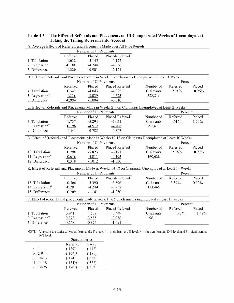
4-13
Table 4-3. The Effect of Referrals and Placements on UI Compensated Weeks of UnemploymentTaking the Timing Referrals into Account
A. Average Effects of Referrals and Placements Made over All Five PeriodsNumber of UI Payments
Referred Placed Placed-Referral1. Tabulation 1.032 -5.145 -6.1772. Regression -0.188 -4.244 -4.0563. Difference 1.220 -0.901 -2.121
B. Effect of Referrals and Placements Made in Week 1 on Claimants Unemployed at Least 1 WeekNumber of UI Payments Percent
Referred Placed Placed-Referral Number of Referred Placed4. Tabulation 0.342 -4.043 -4.385 Claimants 2.28% 0.26%5. Regressiona 1.336 -3.039 -4.375 328,8156. Difference -0.994 -1.004 -0.010
C. Effect of Referrals and Placements Made in Weeks 2-9 on Claimants Unemployed at Least 2 WeeksNumber of UI Payments Percent
Referred Placed Placed-Referral Number of Referred Placed7. Tabulation 1.737 -5.294 -7.031 Claimants 4.61% 1.60%8. Regressionb 0.196 -4.512 -4.708 292,6779. Difference 1.541 -0.782 -2.323
D. Effect of Referrals and Placements Made in Weeks 10-13 on Claimants Unemployed at Least 10 WeeksNumber of UI Payments Percent
Referred Placed Placed-Referral Number of Referred Placed10. Tabulation 0.298 -5.823 -6.121 Claimants 2.76% 0.77%11. Regressionc -0.616 -4.811 -4.195 169,02812. Difference 0.318 -1.012 -1.330
E. Effect of Referrals and Placements Made in Weeks 14-18 on Claimants Unemployed at Least 14 WeeksNumber of UI Payments Percent
Referred Placed Placed-Referral Number of Referred Placed13. Tabulation 0.506 -5.390 -5.896 Claimants 3.39% 0.92%14. Regressiond -0.297 -4.249 -3.952 133,46515. Difference 0.209 -1.141 -1.350
F. Effect of referrals and placements made in week 19-26 on claimants unemployed at least 19 weeksNumber of UI Payments Percent
Referred Placed Placed-Referral Number of Referred Placed1. Tabulation 0.941 -4.508 -5.449 Claimants 4.96% 1.48%2. Regressione 0.373 -3.585 -3.958 98,1113. Difference 0.568 -0.923 -1.491
NOTE: All results are statistically significant at the 1% level; * = significant at 5% level, + = not significant at 10% level, and † = significant at10% level.
Standard errorReferred Placed
a. 1 (.179) (.416)b. 2-9 (.109)* (.181)c. 10-13 (.174) (.327)d. 14-18 (.174)+ (.328)e. 19-26 (.170)† (.302)

4-14
Indeed, comparing the tiny effect of referrals not leading to placements on weeks of UIpayments to the far larger effect on weeks of unemployment suggests the following: obtaininginformation from PLXs that does not lead to direct placements primarily helps claimants to find jobsquickly at the point benefits are exhausted or are close to exhausted. This pattern is highly consistent withconceptual and empirical analyses of how UI benefits affect job search. These studies suggest UI benefitssubstantially raise the minimum acceptable wage of jobs, until benefits are close to exhaustion.
Finally, because the figures in column 1 are so close to zero, subtracting these estimatesfrom those in column 2 makes little difference on the per-person effect shown in column 3. The primaryimpact of assuming a zero effect of information not leading to placements stems from greatly reducing thenumber of claimants helped by PLX direct placement services.
4.3.3 Total Benefits of Referrals and Placements
Obtaining estimates of the per-person effects of PLX direct placement assistance is a keycomponent of a larger goal—determining the total benefits of these services to claimants. Thus, the nextstep in the analysis is multiplying the per-person estimates shown in Tables 4-2 and 4-3 times the numberof individuals affected to estimate the total benefits.
Line 1 of column 1 of Table 4-4 shows that there were 47,555 incidents of claimants beingplaced at jobs (according to our database) from 1987 through mid-1995.4 Line 2 shows that, on average,each placement reduced the duration of joblessness by 9.867 weeks. Line 3 shows that, in total, placedclaimants were jobless by 469,225 fewer weeks (9.867 x 47,555).
4 Because the same claimant can be placed during several different spells of unemployment and even more than once during different periods in a
single spell, the unit of observation technically is the person-period. We use the term incident to indicate that it is possible for the same personto be placed multiple times.

4-15
Table 4-4. Four Measures of Total Benefits Stemming from Claimants’ Decreased Joblessness
Placed versusnot referred
(1)
Referred not placedversus not referred
(2)
Placed versusreferred not placed
(3)
Referred versusnot referred
(4)1 Incidents 1987 - mid 1995 47,555 160,945 47,555 208,500
(col 1 + col 2) (col 1 + col 2)2 Reduction in joblessness 9.867 2.149 7.718 1.000
each incident (weeks) (col 1 - col 2) (assumption)
3 Total reduction in weeks of 469,225 345,871 367,029 208,500joblessness (line 1 x line 2)
4 Average weekly earnings $260 $260 $260 $260quarter after reemployment
5 Total earnings gain $121,998,548 $89,926,409 $95,427,667 $54,210,000(line 3 x line 4)
6 Total gain placed + referred $211,924,957 - $95,427,667 $149,637,667(Line 5, col 1 +
line 5, col 2)(Line 5, col 1 +
0)(Line 5, col 3 +
line 5, col 4)
7 Gain per year (line 6 / 8.5) $24,932,348 - $11,226,784 $17,604,431
Column 4 shows that the average weekly earnings of those placed in the first full quarterfollowing their return to work was $260. Using this amount as the average weekly gain in earnings, weshow in line 5 that the total increase in earnings is $121,998,548. We feel that this is a conservativemeasure of the total gain in earnings because returning to work sooner boosts both current and futureearnings, but we ignore gains that accrue while the claimant is employed.5
Column 2 presents the same calculation as in column 1 for referrals not leading toplacements. The total gain to those referred but not placed is $89,926,409, which is only 74 percent of thegain accruing to those placed. The gain is smaller, although there are 3.4 times more referrals not leadingto placements than placements, because the per-incident reduction in weeks of joblessness is 4.6 timesgreater for placements than for referrals not leading to placements.
5 In the future, we recommend adapting the technique developed by Drs. LaLonde, Sullivan, and Jacobson to directly estimate earnings gains
using administrative data, rather than using this indirect method. However, for the new results to be accurate they need to explicitly take thedecrease in joblessness into account. Because there is a strong negative association between reemployment earnings and unemploymentduration, reducing the duration of unemployment is likely to substantially increase future earnings over what they otherwise would be. This isparticularly true because many of the placements occur after claimants have been jobless for extended periods.

4-16
As shown on line 6 of column 1, adding the total gains from placements and referrals notleading to placements leads to a net gain of $211,924,957. This equals about $25 million a year, which isroughly the cost of running the entire Washington PLX.
Column 3 of Table 4-4 presents lower-bound estimates based on assuming that (a) the valueof referrals not leading to placements is zero; (b) the positive value shown on line 2, column 2, measuresselection bias; and (c) the selection bias for those placed is equal to the bias for those referred but notplaced. Thus, the incidence of placement is the same in column 3 and column 1, the per-incidentreduction in joblessness for those placed is 7.718 (9.867 - 2.149), and the reduction in joblessness forthose placed is 0 (2.149 - 2.149).
The total lower-bound gain in earnings is $95,427,667, which is 45 percent of the gainshown in column 1, and roughly 45 percent of the cost of running the entire Washington PLX. However,we estimate that claimants receive less than 30 percent of all PLX services. Thus, these services have abenefit-cost ratio of about 1.5, which is quite respectable.
However, we believe that the per-incident estimate used here to produce the lower-boundestimate is highly conservative. This view stems from the mail survey results shown in Chapter 3 beingabout the same as those shown on line 2 of column 3, but (a) economic conditions during the periodincluded in this study were considerably worse than in 1998 the period for which the mail survey resultsapply, and (b) evidence shown in the next section indicates that the per-person benefits are about 40percent greater in periods of high unemployment than when unemployment is low.
Moreover, we believe that the per-incident value of referrals not leading to placements isgreater than zero. Even if the reduction in joblessness is only 1 week, column 4 of Table 4-4 shows thatthe benefit from information not leading to placement would equal $54,210,000. When added to thebenefit from being placed the total benefits equal $149,637,667, which is about 70 percent of the totalcost of running the Washington PLXs.
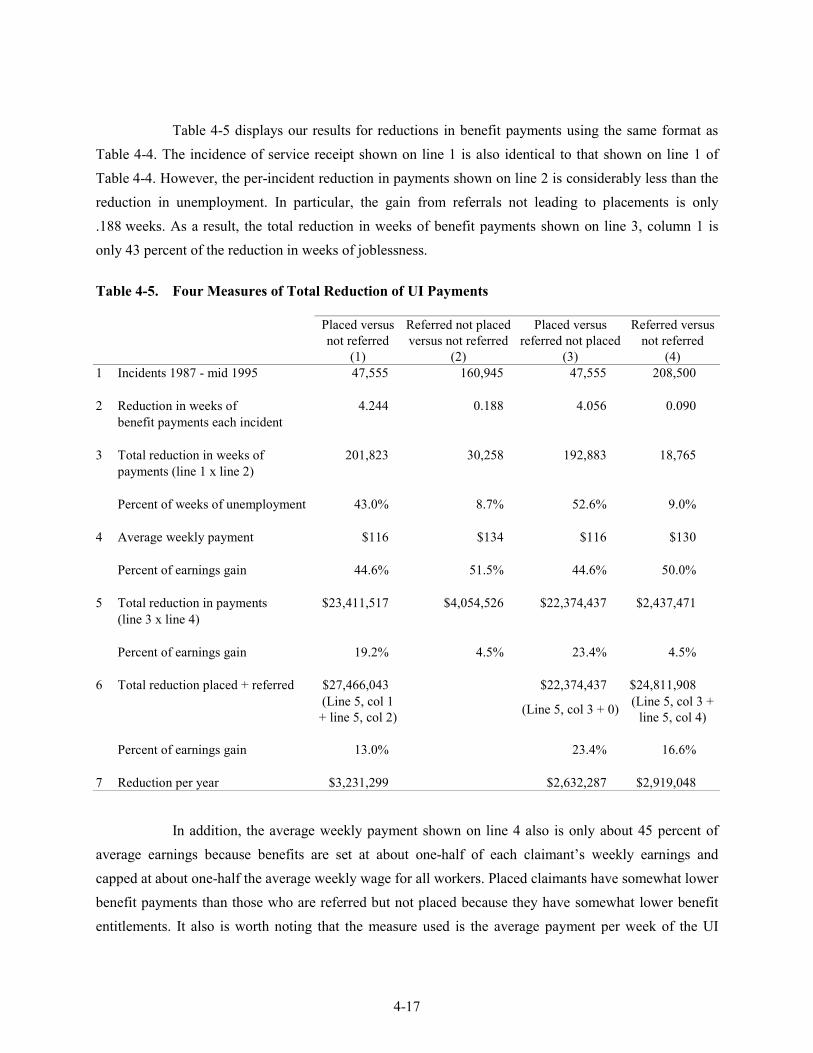
4-17
Table 4-5 displays our results for reductions in benefit payments using the same format asTable 4-4. The incidence of service receipt shown on line 1 is also identical to that shown on line 1 ofTable 4-4. However, the per-incident reduction in payments shown on line 2 is considerably less than thereduction in unemployment. In particular, the gain from referrals not leading to placements is only.188 weeks. As a result, the total reduction in weeks of benefit payments shown on line 3, column 1 isonly 43 percent of the reduction in weeks of joblessness.
Table 4-5. Four Measures of Total Reduction of UI Payments
Placed versusnot referred
(1)
Referred not placedversus not referred
(2)
Placed versusreferred not placed
(3)
Referred versusnot referred
(4)1 Incidents 1987 - mid 1995 47,555 160,945 47,555 208,500
2 Reduction in weeks of 4.244 0.188 4.056 0.090benefit payments each incident
3 Total reduction in weeks of 201,823 30,258 192,883 18,765payments (line 1 x line 2)
Percent of weeks of unemployment 43.0% 8.7% 52.6% 9.0%
4 Average weekly payment $116 $134 $116 $130
Percent of earnings gain 44.6% 51.5% 44.6% 50.0%
5 Total reduction in payments $23,411,517 $4,054,526 $22,374,437 $2,437,471(line 3 x line 4)
Percent of earnings gain 19.2% 4.5% 23.4% 4.5%
6 Total reduction placed + referred $27,466,043 $22,374,437 $24,811,908(Line 5, col 1+ line 5, col 2) (Line 5, col 3 + 0) (Line 5, col 3 +
line 5, col 4)
Percent of earnings gain 13.0% 23.4% 16.6%
7 Reduction per year $3,231,299 $2,632,287 $2,919,048
In addition, the average weekly payment shown on line 4 also is only about 45 percent ofaverage earnings because benefits are set at about one-half of each claimant’s weekly earnings andcapped at about one-half the average weekly wage for all workers. Placed claimants have somewhat lowerbenefit payments than those who are referred but not placed because they have somewhat lower benefitentitlements. It also is worth noting that the measure used is the average payment per week of the UI

4-18
covered spell. This amount is considerably smaller than the maximum weekly benefit payment becausemost spells include at least 1 week with no payments and often include a few weeks where payments arereduced due to having some earnings.
The total reduction in benefit payments is $23,411,517, which is only 19 percent of theearnings gain. Thus, about one-fifth of the placed claimants’ gain in earnings is offset by a loss of UIbenefits over the first 26 weeks of UI spells. If we add the reduction in benefit payments accruing toreferred but not placed claimants shown in column 2 of Table 4-5, the total reduction increases by only17.3 percent to $27,466,043. Because the per-incident referral effects are so small, the lower-boundestimate shown on line 5 is only 20 percent less than the estimate shown in column 3. Similarly, assumingthat referrals not leading to placements have one-half of the measured effect (and one-half is due toselection bias) does not change the estimate of total benefits very much.
4.3.4 Sensitivity Tests
Because the above results appear to produce a plausible range of estimates, we took severalsteps to determine how sensitive the results are to changes in the way the data are organized andequation 4.1 is specified. Probably our most important test is examining the effect of excluding from ourestimates the 11 percent of the spells that do not end with reemployment. This exclusion reduced theaverage affect of referrals not leading to placements and placements on total unemployment by about 10percent.
The effect was large enough to raise concerns that many of those not referred who do notreturn to work may be employed in sectors uncovered by Washington wage record data. Uncoveredsectors include all work in other states, self-employment, government employment, and small farmemployment. However, the duration of benefit collection of not referred claimants who did not return tocovered employment also was exceptionally long. Since any type of employment should terminate benefitcollection, we concluded that most of these individuals were not employed. Thus, on balance, it appearedthat including those not reemployed was reasonable because PLXs were particularly effective in helpingclaimants who otherwise would be unlikely to find work on their own.
We also estimated the effect of referrals and placements for claimants who changed jobs andseparately for those who were recalled. Adding the results together produced results very similar to those

4-19
when both groups were included in a single equation. Also, as expected, the effect of referrals andplacements was much greater for employer-changers than recalled claimants. Even more importantly, theresults supported the view that our estimates were not strongly affected by selection bias. In particular, theeffect of referrals on recalled claimants was about zero, which seems reasonable for a group that mostlyreturns to work within 10 weeks.
We also examined how robust the results are with respect to changes in the specification ofequation 4.1. Our basic finding was that the results change very little, not just when one or two variableswere omitted but also when entire groups were omitted.
Basically, controlling for three characteristics—reemployment status (recall, job change, notreemployed), how long the claimant has been unemployed when a referral is made, and the year theunemployment spell begins—produces referral and placement results that are quite similar to when theentire array of variables are included. Adding industry, earnings, sex, and tenure improves the explanatorypower of the unemployment duration estimates, but has little affect on the referral and placementestimates. Most likely, these added characteristics do not vary much across those placed, referred but notplaced, and not referred, once the first three characteristics are taken into account.
That it is only necessary to control for a few characteristics makes it easy to use equation 4.1for monitoring ongoing operations and replicate the Washington results in other states. However, therobustness tests also showed that the labor market variables we used were insufficient to eliminate theneed to use dummy variables for each individual year in order to capture year-to-year differences ineconomic conditions and other factors. Thus, we doubt that our equations could be used to accuratelyproject the returns to referrals and placements into periods where economic conditions are different fromthose observed.
This means that accurate estimates of current year PLX performance can be based on pastyears’ performance, if labor market conditions and other factors are similar. But if there are majorchanges in labor market conditions, reasonably accurate results would have to wait until sufficient timeelapses to follow up claimants who are placed and referred. Six quarters of followup certainly would besufficient, but additional research is needed to determine if shorter periods would produce accurateresults.

4-20
4.3.5 Other Evidence Bearing on the Effectiveness of PLX Services
When we started to accurately estimate the benefits of PLX referrals and placements, weknew that there were formidable technical problems that make this a very difficult task. Our majorconcerns were:
1. Dealing with negative selection bias at the start of claims periods where claimantswith the poorest prospects of finding work are most likely to seek help from a PLX.
2. Dealing with positive selection bias that occurs after 8 or more weeks ofunemployment when claimants using PLXs may be searching harder for work by avariety of means and are much more likely to accept job offers than apparentlyidentical nonusers.
3. Accurately measuring the duration of joblessness after benefit collection ends.
Our primary concern was measuring the effect of referrals not leading to placements. If thetrue value of PLX referrals is zero, but claimants searching for work use PLXs as one of many differentmeans to find work, the quicker return to work of those referred solely would be a result of search effortbeing correlated with the intensity of PLX use. Thus, it is possible that all of the referral effect is due tomeasurement bias.
However, it is much harder to explain how large placement effects could be due tomeasurement error, especially when referral effects are small. Indeed, it is likely that, if anything,measurement bias is greater for referrals not leading to placements than for those that lead to placements.Thus, we regard the evidence that referral effects are small as very important evidence that there is littlebias in the placement measurements.
Although it seems self-evident that placements should have relatively large effects, there isadditional evidence that it is PLX aid that causes this effect—that large proportions of claimantseventually placed previously spent a lot of time obtaining referrals. If placed claimants are simplysearching harder using a variety of means, and PLX services are of little, if any, value, we would expectthat most of these claimants would find jobs by those other means.

4-21
As shown in Table 4-6, almost two-thirds of the claimants placed after the tenth week ofunemployment were previously referred to jobs by PLXs, and about 50 percent were referred in theprevious 4 weeks. Similarly, the fact that about 45 percent of those referred but not placed in one periodpreviously obtained referrals from PLXs suggests that this activity also is of considerable value.Otherwise, we would expect that claimants might accept referrals once, but not continue to obtainreferrals.
Table 4-6. PLX Use Before Being Placed, Referred, and Being Unemployed During Weeks 1, 2 to9, 10 to 13, 14 to 18, and 19 to 26 of UI Claim Spells
Placed Referred All GroupsNumber Distribution Number Distribution Number Distribution
Week 19 to 26Referred week 14-18 656 45.3% 1,525 25.1% 5,348 5.5%Referred before 14-18 266 18.4% 1,273 20.9% 7,923 8.1%No prior referrals 526 36.3% 3,282 54.0% 84,840 86.5%Total 1,448 100.0% 6,080 100.0% 98,111 100.0%
Week 14 to 18Referred week 10-13 601 49.0% 1,477 24.4% 5,994 4.5%Referred before 10-13 242 19.7% 1,244 20.6% 8,600 6.4%No prior referrals 383 31.2% 3,320 55.0% 118,871 89.1%Total 1,226 100.0% 6,041 100.0% 133,465 100.0%
Week 10 to 13Referred week 2-9 842 65.1% 2,543 39.7% 12,975 7.7%Referred before 2-9 27 2.1% 210 3.3% 1,927 1.1%No prior referrals 425 32.8% 3,658 57.1% 154,126 91.2%Total 1,294 100.0% 6,411 100.0% 169,028 100.0%
Week 2 to 9Referred week 1 1,342 28.7% 2,209 13.0% 7,184 2.5%Referred before 1 – 0.0% – 0.0% – 0.0%No prior referrals 3,339 71.3% 14,804 87.0% 285,493 97.5%Total 4,681 100.0% 17,013 100.0% 292,677 100.0%
Week 1 862 7,015 320,938
NOTE: See Appendix sections C.2 and C.3 for regression estimates
Further, the tendency for claimants to persist with use of the PLX until they find worksuggests that there is a group of claimants who would be unlikely to find work if they were not placed bythe PLX. Indeed, part of the large reduction in total unemployment easily could stem from nonusers beingso discouraged about finding work that they stop looking for work for long periods. In contrast, PLXreferrals encourage users to continue to search for work.

4-22
However, because substantial numbers of claimants find jobs on their own in the sameperiod they receive their first referral, we cannot rule out the possibility that some of the positive effect ofreferrals is due to the type of bias we are attempting to eliminate entirely. Also, some claimants maycontinue to use PLXs purely to satisfy work-search requirements. Thus, our bottom line is that assumingall of the positive effect of referrals is due to measurement bias produces conservative estimates of thetrue effect.
4.4 Results for Each Year
Given that the estimates based on equation 4.1 provide useful information about the benefitsfor all years together, it makes sense to extend the analysis to examine how benefits and costs vary byyear. This is particularly important because (a) benefits are likely to vary substantially with differences ineconomic conditions, and (b) today’s strong economic conditions differ radically from those of the 1991-92 recessions and their aftermath that heavily affect the results presented above.
Precisely the same steps used for examining all years together are used to examine each yearindividually. First, we estimate the per-person effect of placements and referrals not leading toplacements. Second, we use estimates of the number of incidents of placements and referrals not leadingto placements to estimate the total reduction in the number of weeks of unemployment and UI payments.Third, we multiply the total number of incidents times average earnings and average payments to estimatetotal benefits.
4.4.1 Per-Person Effects by Year
Table 4-7 (a and b) displays the same measures of the effects of referrals and placements onUI payments and weeks of unemployment presented in Tables 4-2 and 4-3, but for each year, rather thanall years together. The year-by-year estimates were derived from introducing separate variables forreferrals and placements in each year into the same specification used for producing all years togetherresults. Separate equations were run for the same five periods relative to the start of the UI claim. The farmore cumbersome alternative of also using separate equations for each year was tried but found toproduce almost identical results.
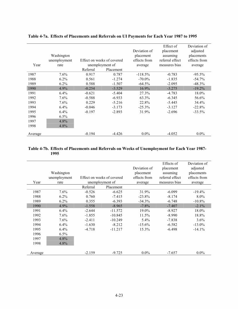
4-23
Table 4-7a. Effects of Placements and Referrals on UI Payments for Each Year 1987 to 1995
Year
Washingtonunemployment
rateEffect on weeks of covered
unemployment of
Deviation ofplacement
effects fromaverage
Effect ofplacementassuming
referral effectmeasures bias
Deviation ofadjusted
placementseffects from
averageReferral Placement
1987 7.6% 0.917 0.787 -118.5% -0.783 -95.5%1988 6.2% 0.561 -1.274 -70.0% -1.835 -54.7%1989 6.2% 0.588 -1.507 -64.5% -2.095 -48.3%1990 4.9% -0.254 -3.529 16.9% -3.275 -19.2%1991 6.4% -0.621 -5.404 27.3% -4.783 18.0%1992 7.6% -0.588 -6.933 63.3% -6.345 56.6%1993 7.6% 0.229 -5.216 22.8% -5.445 34.4%1994 6.4% -0.046 -3.173 -25.3% -3.127 -22.8%1995 6.4% -0.197 -2.893 31.9% -2.696 -33.5%1996 6.5%1997 4.8%1998 4.8%
Average -0.194 -4.426 0.0% -4.052 0.0%
Table 4-7b. Effects of Placements and Referrals on Weeks of Unemployment for Each Year 1987-1995
Year
Washingtonunemployment
rateEffect on weeks of covered
unemployment of
Deviation ofplacement
effects fromaverage
Effects ofplacementassuming
referral effectmeasures bias
Deviation ofadjusted
placementseffects from
averageReferral Placement
1987 7.6% -0.526 -6.625 31.9% -6.099 -19.4%1988 6.2% 0.760 -7.415 -23.8% -8.174 8.0%1989 6.2% 0.355 -6.393 -34.3% -6.748 -10.8%1990 4.9% -1.558 -8.965 -7.8% -7.407 -2.1%1991 6.4% -2.644 -11.572 19.0% -8.927 18.0%1992 7.6% -1.855 -10.845 11.5% -8.990 18.8%1993 7.6% -2.411 -10.249 5.4% -7.838 3.6%1994 6.4% -1.630 -8.212 -15.6% -6.582 -13.0%1995 6.4% -4.718 -11.217 15.3% -6.498 -14.1%1996 6.5%1997 4.8%1998 4.8%
Average -2.159 -9.725 0.0% -7.657 0.0%

4-24
In reviewing these results, it is important to keep in mind that the standard errors of theestimates are much greater than when the results are not disaggregated. The standard errors are largerelative to the small effects of referrals on covered unemployment but still very small relative toplacement effects. Thus, some of the variation, particularly in referral effects, is due to samples forindividual years being roughly one-tenth the size of the sample for all years together.
Also, the results for the earliest and latest years are affected by not having long strings ofpre- or post-unemployment wage records. The 1987 and 1995 results are strongly affected by mostclaimants not having the wage records needed to determine recall and job change. In addition, the late1994 and 1995 results are affected by the short followup period preventing accurate estimation of theduration of unemployment. When claimants did not return to work we assumed that they wereunemployed for 83 weeks. This assumption is responsible for the exceptionally large estimated effect of1995 referrals on total unemployment.
The year-by-year results are in keeping with expectations, once we recognize themeasurement problems with the earliest and latest years. The effects of referrals and placement on UIpayments and unemployment are greatest during 1991-1993, years strongly affected by recessions. In thatperiod placement effects are about 30 percent above average on weeks of UI payments and about12 percent above average on total weeks of unemployment.
The effect on benefit collection duration is more than twice that on unemployment durationbecause UI payments were extended by a series of Federal programs in the aftermath of the 1991-92recessions. The extended benefit programs extended collection from about 26 weeks to a minimum of52 weeks and, in some cases, as many as 121 weeks. Thus, extended benefits (1) reduced the probabilitythat spells ended with UI exhaustion, and (2) decreased incentives for claimants to take the best jobs thatwere available, rather than remain jobless.
Thus, it is hardly surprising that the effects of placements on covered unemployment were solarge during the period extended benefit programs were in place. Also, it seems reasonable that the effectswould fall from a peak of 6.9 weeks to below 3.0 weeks as economic conditions improved and theextended benefit programs were terminated. Importantly, 1990 economic conditions appear to have beensimilar to conditions in 1997-98. This suggests that current benefits are much lower than those duringrecessions but still substantial.

4-25
It also makes sense that as economic conditions improve, the decline in benefit paymentsand unemployment duration due to placements are comparable in terms of weeks. But the decline as apercentage of average is far lower for weeks of unemployment than weeks of payments. This result stemsfrom (a) PLX placement services strongly affecting claimants who otherwise would be unemployed forsubstantial periods without PLX aid in both good times and bad, and (b) the measure of benefit paymentsbeing heavily influenced by extended benefit programs that only are in effect during bad periods. Thus,while improvement in economic conditions affects those with the greatest difficulty finding work, theperiod over which those improvements can be observed is far shorter in the absence of extended benefitprograms.
Referral effects show similar patterns to those for placements, but in several cases referralsappear to increase, rather than reduce, collection of benefits. Although it is unlikely that referrals makeclaimants worse off, obtaining small positive estimates is not especially surprising because most of theeffects are close to zero, and it is difficult to control for the poor prospects of finding work that usuallyprompts use of PLXs in the first place.
4.4.2 Number of Claimants Referred and Placed Each Year
Table 4-8 provides year-by-year information about the number of claimants in our sample,the number referred and placed claimants in our sample, and the ratio of claimants in our database to thenumber of claimants reported in official statistics.
The ratio of the number of claimants in our database (multiplied times five to reflect thesampling ratio) relative to the number of UI first pays is presented in the box on the bottom right ofTable 4-8. These figures show that our sample is complete from 1990 through 1994. We expect that oursample will be greater than first payments because each claimant enters the sample each time he or sheestablishes a new claim, while first pays reflect the establishment of a new benefit year that can onlyoccur once in a calendar year. The pattern of differences is consistent with the effect of worseningemployment prospects and triggering of extended benefit programs on the number of separate spells ofunemployment.

4-26
Table 4-8. Number and Distribution of Referrals, Placements, and Claimants; Comparison ofClaimants in the Database to UI First Payments for Each Year 1987 to 1995
Number of:
Year
Referrals(not leading to
placements) PlacementsClaimants
(spell starts)
Referrals as apercent ofclaimants
Placements as apercent ofclaimants
1987 182 175 20,058 0.9% 0.9%1988 514 364 18,034 2.9% 2.0%1989 1,272 637 19,943 6.4% 3.2%1990 3,775 1,274 32,329 11.7% 3.9%1991 5,709 1,588 50,318 11.3% 3.2%1992 5,874 1,553 53,968 10.9% 2.9%1993 6,047 1,501 57,441 10.5% 2.6%1994 5,771 1,527 52,172 11.1% 2.9%1995 3,026 892 24,553 12.4% 3.6%
Total 32,190 9,511 328,815Average 9.8% 2.9%
Distribution of: Claimants in the
Year
Referrals(not leading to
placements) PlacementsClaimants
(spell starts)
database as apercent of first
payments
Placements as apercent allReferrals
1987 0.6% 1.8% 6.1% 66.2% 49.0%1988 1.6% 3.8% 5.5% 56.8% 41.5%1989 4.0% 6.7% 6.1% 67.7% 33.4%1990 11.7% 13.4% 9.8% 89.3% 25.2%1991 17.7% 16.7% 15.3% 100.7% 21.8%1992 18.2% 16.3% 16.4% 107.8% 20.9%1993 18.8% 15.8% 17.5% 114.1% 19.9%1994 17.9% 16.1% 15.9% 102.8% 20.9%1995 9.5% 9.4% 7.5% 61.7% 22.7%
Total 100.0% 100.0% 100.0%Average 91.8% 22.8%

4-27
The 1995 shortfall also is in keeping with expectations because we excluded from thisanalysis claimants who had not exhausted their benefit entitlement by the end of 1995. However, theshortfalls for 1987-89 suggest that our sample is not complete for those years. Discussions withWashington State officials suggest that the most likely reason for these shortfalls is that some data werenot archived when a new management information system was installed during this period.
The 1987-88 data problems clearly extend to referrals and placements. In those yearsreferrals, and to a somewhat lesser extent placements, as a percentage of claimants are disproportionatelylower than in other years. For example, 1987 claimants constitute 6.1 percent of all claimants, but 1987referrals constitute on 0.6 percent of all referrals, and 1987 placements are 1.8 percent of all placements.
We decided to include the 1987 and 1988 data in the study because there are so fewplacements and referrals in these years that they have a very small effect on the total results. At the sametime, their inclusion points up the problems with going back over a long period to retrieve data, as well asthe problem with drawing inferences from data covering the first year of a series.
In contrast, referral and placement data for 1995 appear to be proportional to the fraction ofclaimants. This suggests that adjusting the 1995 service data to compensate for the shortfall wouldprovide an accurate measure of total benefits. However, we decided not to adjust the 1995 estimatesbecause the per-person effect measures are inaccurate due to the followup period being constrained. Akey message from this evidence is that it might take states a few years from the point they begin toassemble data needed to monitor PLX operations to the point they can be confident results are reasonablyreliable. This puts a premium on starting as quickly as possible.
4.4.3 Total Benefits and Costs by Year
Tables 4-9a and 4-9b display the benefits from referrals and placements reducing UIpayments and total unemployment, respectively. The computations were made precisely as they were forall-years-together in Table 4-9c. We multiplied the average effect measured in weeks times the number ofinstances times the per week decrease in UI payments or increase in earnings. We also used the samemeasures of weekly UI payments and weekly earnings across all years because the differences onceinflation was taken into account were small.

4-28
Table 4-9a. Total Yearly Gains from Referrals and Placements Reducing UI Payments
Reduction in UI payments Due to:Year Referral Placement Both
Distribution ofreductions
Reductionassuming referraleffect measures
biasDistribution of
reductions
1987 $118,362 $79,916 $198,278 -0.7% -$18,605 0.1%1988 $193,330 -$268,863 -$75,324 0.3% -$387,383 1.7%1989 $501,039 -$556,697 -$55,659 0.2% -$773,906 3.5%1990 -$641,683 -$2,607,369 -$3,249,052 11.8% -$2,419,901 10.8%1991 -$2,376,251 -$4,977,062 -$7,353,313 26.6% -$4,404,878 19.7%1992 -$2,314,734 -$6,245,097 -$8,559,831 31.0% -$5,715,322 25.6%1993 $925,872 -$4,540,970 -$3,615,099 13.1% -$4,739,921 21.2%1994 -$178,815 -$2,810,088 -$2,988,903 10.8% -$2,769,129 12.4%1995 $402,860 -$1,496,761 -$1,899,621 6.9% -$1,394,634 6.2%Total -$4,175,742 -$23,422,992 -$27,598,734 100.0% -$22,354,940 100.0%
Table 4-9b. Total Yearly Earning Gains from Referrals and Placements
Increase in earnings due to:Year Referral Placement Both
Distribution ofincreases
Increaseassuming referraleffect measures
biasDistribution of
increases1987 $124,392 $1,507,137 $1,631,529 0.8% $1,387,529 1.5%1988 -$507,509 $3,508,567 $3,001,058 1.4% $3,867,970 4.1%1989 -$586,983 $5,294,414 $4,707,431 2.2% $5,588,367 6.0%1990 $7,646,484 $14,847,554 $22,494,038 10.7% $12,266,992 13.1%1991 $19,626,494 $23,888,459 $43,514,953 20.7% $18,429,206 19.7%1992 $14,162,863 $21,894,789 $36,057,653 17.1% $18,150,335 19.4%1993 $18,955,583 $19,999,246 $38,954,829 18.5% $15,294,047 16.3%1994 $12,229,407 $16,301,093 $28,530,500 13.5% $13,065,206 14.0%1995 $18,684,265 $13,006,677 $31,690,942 15.0% $7,535,120 8.1%
Total $90,334,997 $120,247,937 $210,582,933 100.0% $93,557,159 100.0%
Table 4-9c. Total Yearly Costs and Benefit-Cost Ratios
Benefits assuming referralsmeasure bias as percent of:
Year PLX Cost
Benefits from referralsand placements as apercent of total cost Total cost
Cost of serving claimants(Estimated at 35% of total)
1987 $25,403,602 6.4% 5.5% 15.6%1988 $25,571,371 11.7% 15.1% 43.2%1989 $25,573,263 18.4% 21.9% 62.4%1990 $26,615,821 84.5% 46.1% 131.7%1991 $26,045,997 167.1% 70.8% 202.2%1992 $26,344,969 136.9% 68.9% 196.8%1993 $25,538,436 152.5% 59.9% 171.1%1994 $26,090,959 109.4% 50.1% 143.1%1995 $24,319,544 130.3% 31.0% 88.5%Total $231,493,961 91.0% 40.4% 115.5%
1990-94 $130,626,182 129.8% 59.1% 168.9%

4-29
The pattern of UI payments reductions across years is similar to the pattern in the number ofreferrals and placements. However, differences between good times and bad are further accentuatedbecause per referral and per placement reductions also strongly fluctuated over the business cycle. (Also,keep in mind that the estimates for 1987, 1988, and 1995 substantially underestimate the true effects, andtherefore, are of limited value.)
Total reductions were above $8.5 million in 1992 and almost as great, $7.3 million, in 1991.In years with much stronger economic conditions and no extended benefit programs, active reductionswere much smaller. In 1990, the study year with the best economic conditions, reductions were $2.6million, which is much lower than in 1991-92 but still substantial. Reductions were only a bit greater $2.8million in 1994. These differences provide further evidence of how much larger payment savings are inperiods when extended benefit programs are active.
Interestingly, assuming that the referral effect purely captures measurement bias does notchange the results very much because referrals usually have small effects and, in some cases, appear tolengthen covered unemployment. Comparing the distributions of benefits using the two methods clearlyshows that assuming that referral effects only reflect measurement bias increases estimates for years withsmall benefits and decreases estimates for years with large estimates. Because it is reasonable to expectthat benefits are proportionally larger when extended benefits programs are active, we feel that at leastsome of the measured effect of referrals is not due to measurement bias. Thus, we remain confident thatassuming that referral effects are due to bias produces highly conservative estimates of the true benefits.
Comparisons between Tables 4-9a and 4-9b show that (a) estimates of earnings gains aremany times larger than estimates of UI payment reductions, (b) earnings increases from referralscontribute importantly to the overall gains, and (c) the differences across years are considerably less forearnings gains than reductions in UI payments.
Earnings gains are greatest, $43.5 million, in 1991, but almost as large in 1992 and 1993,$36.1 and $39.0 million, respectively. The gain in 1990, the year with the best economic conditions, is$22.5 million. This is roughly one-half the gain in 1991, the peak year. Most of the decline stems from aone-third reduction in the number of claimants, but some of it stems from a substantial decline in the per-person effect of referrals and placements.

4-30
Assuming that referral effects measure bias reduces the estimates of earnings gains by about45 percent on average. However, the gains are still large. Also, the conservative assumption produces amuch more reasonable estimate for 1995, a year when many claimants beginning spells were omitted.
This is an interesting result because the estimated referral effect for 1995 is exceptionallylarge and it is the only year where results may be strongly biased by not having a long enough followupperiod (and having to make an assumption about how long claimants were jobless). Thus, it is reasonableto believe that the bias correction may only make sense for this year alone. Additional evidence that biasis confined to 1995 earnings reduction estimates comes from the facts that (a) referral effects on coveredunemployment are not especially large for 1995, and (b) covered duration is known with precision.
Finally, the first column of Table 4-9c shows the total budget for Washington PLXs in eachyear. These estimates include Wagner-Peyser funds, state claimant placement program funds, and veteranprogram funds, which account for two-thirds, one-sixteenth, and one-sixth of the budget, respectively.
Unfortunately, it is very difficult to determine how much of the funds were spent on directplacement services for claimants (during the period they were collecting benefits). However, we knowthat budgets do not fluctuate much from year to year. This suggests that much of the cost of directplacement services is the relatively fixed cost of maintaining the computer matching system andproviding staff to assist PLX-users.
A ballpark estimate is that roughly 35 percent of the PLX budget goes to providingplacement services to the claimants during the first 26 weeks they collected benefits. This figure is basedmainly on our estimate that nonclaimants make up about 60 percent of PLX users, but also takes intoaccount the fact that claimants often receive services other than those leading to direct placements. Inparticular, substantial amounts of staff time go to conducting workshops, providing counseling, andmaking referrals to alternative services.
Clearly, the gains in earnings accruing to claimants are very impressive even when measuredagainst total PLX outlays. Over all years the benefits equal 91 percent of costs, and lower-boundestimates indicate that the benefits equal at least 40 percent of the costs. These are remarkably largenumbers given that the true incidence of service receipt is severely underestimated for 1987 and 1988,and somewhat underestimated for 1989.

4-31
When we restrict the estimates to the years for which we are most confident they areaccurate, 1990-94, the gains are truly remarkable. Including the value of referrals produces estimates thatbenefits equal 130 percent of costs for that period. Even assuming that referral estimates represent bias,benefits amount to about 60 percent of costs.
Admittedly, most of the period covered was in recession, when finding jobs was particularlydifficult and extended benefit programs further reduced incentives to find work. However, the resultswere unaffected by extended benefits in 2 of the 5 years, 1990 and 1994, and economic conditions weregood in 1990 and improving in 1994. Also, the true incidence of aid given to claimants most likely isunderstated for 1990.
While results for 1987-89 are much smaller than for later years, we are certain that theincidence of referrals and placements is so severely underestimated that the 1987-88 figures aremeaningless. Comparisons with official statistics suggest that the incidence of claims is underestimatedby at least 50 percent for 1989. While taking this difference into account does not bring the results up to1990 levels, it brings them close enough to suggest that some other data problem is the source of thesmaller estimates for 1989.
We, therefore, conclude that even in relatively good economic times the benefits toclaimants are about 100 percent of the costs assuming our estimates are unbiased. At a minimum, benefitsare 50 percent of costs, which is still considerably greater than outlays to produce the benefits.
4.5 Summary and Conclusions
This chapter used an exceptionally large administrative database covering an unusually longperiod to determine:
How well these data measure the effect of PLX placements and referrals on UIclaimants’ job search and benefit collection.
Whether the techniques used here can and should be used on an ongoing basis toprovide meaningful feedback to program operators and policymakers.

4-32
The analysis presented in this chapter provides highly positive assessments of both issues. Inparticular, the analysis suggests that:
1. On average, placements reduce the duration of unemployment by 7.7 weeks relative tobeing referred but not placed. This nonexperimental estimate of the per-incident effectof placements relative to obtaining referrals are similar to those generated from use ofa survey. While several steps should be taken to increase our confidence that theseresults reflect those from a natural experiment, we feel that the bias in these results issmall enough for the similarity to support the view that the non-experimentalestimates are reasonably close to the true values.
2. We produced plausible nonexperimental estimates of the per-incident effect ofobtaining information in the course of being referred relative to not being referred,and usually not obtaining any PLX help, even though we have no experimentalevidence to serve as a benchmark. On average, our procedures produce estimates thatreferrals reduce the duration of unemployment by 2.1 weeks relative to not beingreferred. Even if measurement error accounts for half of this figure, the contribution tototal benefits is large.
3. Estimates of the total benefits hinge on multiplying the per-incident effect times thenumber of incidents and average weekly post-unemployment earnings.
a. The administrative data provided accurate estimates of the incidence of beingplaced and being referred once the state employment security agency decided touse these data for in-depth analysis. On average, PLXs refer about 25,000claimants per year, of whom about 7,000 are placed.
b. Our procedure for estimating post-unemployment earnings is reasonablyaccurate, but could be greatly improved by applying techniques used with theseadministrative data in estimating the earnings losses due to job loss. Post-unemployment earnings of claimants average about $260 per week.
4. Estimates of the year-by-year variation in the pre-incident effect of placements andreferrals as well as the total benefits derived from direct placement services are muchin keeping with expectations. Total benefits are between 30 and 40 percent greater inthe trough of a business cycle than near its peak.
a. About one-third of the peak-to-trough reductions are due to reductions in theper-incident effect of placements and referrals as economic conditions improve.Placements, in particular, are more potent when good jobs are more difficult tofind and extended benefit programs considerably lengthen the period overwhich UI can be collected.
b. About two-thirds of the reductions are due to there being fewer claimants intotal during prosperous periods.
5. The cost of running the entire PLX system in Washington is easily derived frombudget figures. Those costs average about $25 million per year and vary very little

4-33
from year to year. Sixty percent of the funds come from the Federal Wagner-Peyserallocation, 15 percent from Federal Veterans funding, and the bulk of the remainderfrom state funds earmarked to assist claimants. It is not nearly as easy to determinehow much of the total goes to providing direct placement services, nor how much ofthose funds goes to aiding claimants. We use a ball park estimate of 35 percent for theportion spent on direct placement services going to claimants included in the benefitcalculations.
6. We produce the following three different benefit-cost estimates:
a. The lowest estimate assumes that the value of the information obtained ingetting referrals is zero. Thus, this measure only includes the value ofplacements relative to being referred but not placed. This produces a benefit-cost ratio of 1.2 (using the 35 percent estimate of the portion of costs going todirect placement services and including 1987-89, and 1995 years for which theincidence of placements and referrals is substantially underestimated).
b. A less conservative estimate assumes that half of the measured referral effect isdue to measurement error. This assumption produces a benefit-cost ratio of 1.9.
c. The least conservative estimate accepts the referral effect measure as beingaccurate. This assumption produces a benefit-cost ratio of 2.8.
Because the per-incident cost of placements and referrals is very low, we feelthat even the least conservative estimate is plausible. Key reasons for this vieware that: (1) receipt of UI payments greatly restricts the types of jobs claimantsare likely to accept before exhausting benefits, (2) some claimants would havegreat difficulty finding suitable work on their own after they have been joblessfor several months and (3) we included 1987-89 and 1995 years for which theincidence of placements and referrals is substantially underestimated. Thus, wethink it is likely that placements and referrals will be particularly potent forclaimants.
The trend in unemployment reductions stemming from placements and referralsobtained after successively longer periods of being unemployed stronglysupports the view that, as unemployment duration lengthens, claimants havemore and more difficulty finding jobs on their own. The per-incident effectsjust about double from between the 9th and 19th week of unemployment spells.
7. Separate estimates suggest that UI payment reductions equal about 22 percent of thegain in earnings. Payment reductions are lower because weekly payments are aboutone-half of weekly earnings and because payments end after about 30 weeks, onaverage. Thus, except during periods covered by extended benefits, reductions in UIpayments are modest relative to the cost of providing direct placement services toclaimants. Nevertheless, employers benefit both from the reduction in UI payments,which usually will reduce their UI tax burden, and from claimants’ increased earnings.By lowering the cost of job loss, placement services reduce “the risk premium”workers would require to take jobs that are likely to end with permanent layoffs.

4-34
Overall, we strongly feel that program operators, policymakers, and concerned citizens of alltypes would be much better off using the type of information described above in assessing theperformance of PLXs than the types of data that have been used to date. Second, we do not think it wouldbe difficult to produce these measures on an ongoing basis.
Of primary importance, comparing benefits to costs is a much better way to judge bothoverall performance and determine ways to improve performance of any program. In particular, it focusesattention on program effects rather than outcomes that often largely have nothing at all to do withprogram effectiveness. Also, use of the more sophisticated value-added measures that require use ofcomparison groups for one program might lead to improving measures and the conceptual framework forviewing other employment and training programs.
Finally, in our view presenting three benefit-cost estimates is not unduly confusing, butrather honestly reflects how difficult it is to overcome key measurement problems. Also of considerableimportance, adoption of the measurement system used here would produce the straightforward measuresthat have been used in the past and improvements on those measures. For example, we could determinethe placement and referral rates as a function of how long claimants were jobless prior to receiving thisaid, and further determine how many referred but not placed claimants were recalled to former jobs.These measures should help put the contributions of PLXs into a far more relevant context than can use ofthe current ETA-9002 measures.
Because we feel that the range of estimates of placement and referral effects provides areasonably accurate view of benefits going to claimants, it is our view that the biggest improvements inPLX measures would come from expanding the above measures to include:
a. Claimants who have stopped collecting benefits;
b. Other unemployed job seekers with strong work records;
c. Unemployed job seekers with spotty work records; and
d. Job seekers searching while employed.
The primary impediment to measuring placement effects for these groups withadministrative data is not knowing for sure when these individuals began to search for work, and if theyfailed to find new jobs, when they stopped searching. Because claimants are supposed to be able,

4-35
available, and have not refused suitable jobs, UI payment data provide a reasonably accurate measure ofperiods of job search. In this study we did not even examine referral and placement effects after claimantsstopped collecting benefits because we were concerned these measures would be biased due to thedifficulty in determining whether claimants are searching for work after they stop collecting benefits.
We think that it should not be too difficult to at least determine the duration of job search tomake reasonably accurate estimates of the effect of being placed relative to being referred but not placedamong members of all four groups. Indeed, the one-time use of a mail survey with telephone followupwould provide a benchmark for developing unemployment duration measures using administrative dataalone, and adjusting nonexperimental estimates to reflect those generated from a natural experiment.
What would be extremely difficult to do is develop job search duration measures forindividuals who could serve as a comparison group of nonreferred individuals who have spotty workrecords or search while employed. Fortunately, even if we omitted these estimates, we would be able toproduce lower-bound estimates for all groups, and less conservative estimates for the vast majority ofreferred individuals. An important, but far less critical, improvement is more accurately translatingreductions in weeks unemployed into increases in earnings, as already noted in point 4a above.
In short, while we consider our estimates to be far from perfect, they dramatically improveon the measures that are currently in use as well as those advocated to replace existing PLX measures.Indeed, in our view the primary threat to greatly improving PLX measurement is instituting self-servicecomputerized systems to review PLX job orders that provide contact information without requesting thatusers register with PLXs and identify which job orders they are likely to pursue.

Chapter 5

5-1
5. DETAILS OF OUR RESEARCH USING OREGON ADMINISTRATIVE DATA
In this chapter, we describe our analysis of the effect of PLX referrals and placements onOregon unemployed insurance (UI) claimants. We do this using a database developed by the OregonEmployment Department (OED) to our specifications. One goal of this work was to see if the largeWashington benefits were typical of results in other states. A second goal was to see if the methods usedfor the analysis could be implemented by a state employment security agency.
Because the design of this work is nearly identical to that just discussed in Chapter 4, we donot need to go into detail about why we limited the study to claimants or explain the conceptualframework for the analysis. Instead, we describe the process by which we developed the analyticdatabase. We then describe our results derived from use of a model that differs only slightly from the onediscussed in Chapter 4. Finally, we summarize what we learned about the effectiveness of placements andreferrals, and how states can develop similar databases for measuring public labor exchange (PLX)effectiveness.
5.1 Database Development
This study was designed to replicate the Washington administrative data analysis as closelyas possible. However, rather than Westat working with raw wage, claim, and PLX files on our owncomputer, as was the case with the Washington analysis, Westat provided detailed descriptions of the dataprocessing steps to the OED, who then performed all the data processing. Westat worked with OEDofficials to check whether the database was properly created and to correct problems. Ultimately, wespecified the analytic model and analyzed the results, but we did not have copies of the person-level filesused to run the regressions described below.
The data processing tasks consisted of the following three elements:
1. Creating an analytic file from the raw files;
2. Ensuring that the analytic file was sound; and
3. Estimating the effect of placements and referrals on claimants’ job search.

5-2
One element did not smoothly follow completion of the preceding element. Some problemswere only spotted at the point estimates were produced and inconsistencies became apparent. Thus, someprograms that we thought were sound had to be refined. Even at the end of the project, it still appearedthat the database did not capture all the services received by claimants.
Overcoming the problems we encountered was part of the normal process of usingadministrative data for in-depth analysis. Similar problems were encountered in our use of data fromWashington and other states. However, given sufficient time and resources it has always been possible toultimately produce a sound analytic database.
Constraints imposed by not being able to validate the models we used with experimentalevidence are far more important impediments to accurately estimating PLX effectiveness than areproblems in creating analytic files. Indeed, we refined our analytic models using the Washington dataconcurrently with developing the Oregon database. In some cases, it was only after we refined our modelsthat some of the problems with the data became apparent.
It is also worth noting that prior to the start of our joint project OED had made a majorinvestment in creating a data warehouse. Thus, the basic “raw” data files needed for this work wereavailable about 2 years ago when our collaboration began. The preliminary steps conducted by OED onits own included:
1. Developing a common format for each type of file across years;
2. Providing excellent documentation for the contents of each file; and
3. Storing the data in a way that made it easy to process.
Having this start saved 3 to 5 months of hard work and reduced expenditures by as much as $300,000.
In order to assist OED in reformatting the data to produce an analytic file, we provided whatwe called “The Cookbook”—a large loose-leaf folder with the precise details of every processing step wecarried out using the Washington data. The new database was created by adapting the information weprovided to the OED’s computer environment.
Much of this work was carried out by OED staffers who had completed or almost completeddoctorates in economics from Oregon State University. Having staff with extensive experience with

5-3
structuring data for analysis and estimating models using statistical packages was a major asset to thisproject and substantially reduced the time and effort needed to produce the results.
After the database was created, we ran tests to determine whether the data were sound. Ourinitial comparisons used a simplified model that suggested that some of the crucial variables were notproperly constructed. We then made minor adjustments to the programs to create variables that appearedto be precisely correct. However, as we got deeper into the analysis, it became clear that we had notcaught all the errors. We, therefore, conducted far more detailed tests of the accuracy of the variables.This led to making extensive modifications to the basic programs.
Finally, we applied even more sophisticated models and produced what appeared to bereasonable estimates of the effects of referrals and placements on claimants’ duration of joblessness andcollection of UI benefits. However, after converting the per-person effects to total effects, we determinedthat the number of referrals and placements in the database were only about one-half of the numberreported in published tables. We were able to accurately estimate total effects, but could not determinewhy the database was incomplete.
The next section summarizes the key lessons we learned about how to make the databasedevelopment process go smoothly.
5.1.1 Lessons for Developing Analytic Files
There are two separate issues in creating sound analytic files:
1. Ensuring that each variable for each person is properly created; and
2. Ensuring that the database includes the right number of individuals in total and theright number of individuals receiving various types of services.
The cookbook we provided had the information needed to properly create each variablebecause it included: (a) a description of each variable, (b) the computer code used to produce the variable,and (c) a detailed printout of how the raw data looked and how the transformed data looked after thecomputer program was run. Unfortunately, OED was not able to simply run the programs we created foruse with Washington data. Instead, they wrote their own programs using a different computer language.

5-4
In such cases, it is imperative to very carefully check how the programs work by looking at the variablesin the input and output files.
Initially, we did not request detailed formatted data dumps, but eventually we had to producethese dumps in order to resolve problems with the data. There is no question that we should haverequested and reviewed the detailed dumps right from the start.
Even if we did not spot problems immediately, having these files would have made it fareasier to resolve issues when they arose. A key problem is that many complex steps had to be completedin order to produce the analytic files, and without a complete set of data dumps at each stage, it wasdifficult to determine at what step something might have gone wrong. Indeed, by the time a questionsurfaced it was common for the person doing the programming to have left OED or be unable to recallprecisely what was done.
Although we believe that our checks ultimately led to properly transforming the variables inthe raw files, we were unable to determine why there were only about one-half of the number of referralsand placements in our database as there were in published statistics. Indeed, we believe that the shortfallswere in the raw files and not due to errors in the way the data were processed. However, this is notcertain. Clearly, we should have made the comparisons between aggregate statistics and tabulations of theraw files and continued to create counts at each stage in the processing to make sure that data continued tobe complete.
One reason that we did not make the detailed comparisons using Oregon data initially is thatwe knew at the outset that (a) Oregon’s labor force was about 60 percent the size of Washington’s; and(b) the number of claimants, referrals, and placements in the Oregon database were roughly 60 percent ofthose in Washington. Unfortunately, what we did not know was that the Oregon PLX job banks includeda far higher proportion of all job vacancies than did the Washington PLX job banks and that Oregonassists a far higher proportion of claimants than does Washington.
A second reason for not making these comparisons is that we assumed that some of thechecks were carried out in the course of creating the data warehouse. However, in retrospect it is obviousthat it is a mistake to take any key assumption for granted. We can not emphasize too strongly that it isessential to assemble relevant published statistics at the outset and determine at each stage that tabulationsof the person-level files match those published statistics.

5-5
5.2 The Per-Incident Effect of Referrals and Placements
The estimating equation used with the Oregon data was almost identical to that used with theWashington data. The only important difference is that the Oregon estimates lacked the final refinementin the Washington model of restricting our measure of the effect of referrals not leading to placements toclaimants who were not placed at any time within 39 weeks of the start of a given unemployment spell.(See Appendix section D.1 for the list of variables.)
The restriction was made because otherwise much of the positive effect attributed to referralsnot leading to placements, in reality, would be due to subsequent placements. Fortunately, this differencedid not have much effect on the measures of total benefits because most Oregon referrals and placementsoccurred before the tenth week of unemployment, and most of those claimants returned to work in thatperiod. Thus, subsequent placements were rare.
Panel A of Table 5-1 presents the key Oregon results. These results cover only one calendaryear, 1995. On average, a referral not leading to a placement reduces the duration of claimants’unemployment by about 1.1 week, and a placement reduces unemployment by about 5.8 weeks.Subtracting the referral effect from the placement effect produces a 4.6-week estimate for the reduction inunemployment following a placement relative to viewing listings and receiving staff assistance but notbeing placed.
As noted in earlier chapters, there is some uncertainty about whether the 1.1-week reductionin unemployment associated with referrals not leading to placements accurately measures the value ofobtaining information that helps claimants decide to take jobs they find on their own and accept offersmade as a result of referrals. It is possible that at least some of this reduction is due to measurement error.Thus, we later display estimates of total benefits with the referral effect included and the effect excluded.
Placement effects (relative to not being referred) increase markedly after the ninth week ofunemployment and then increase markedly again after the 18th week. This pattern, coupled with the factthat almost three-quarters of all claimants return to work by the tenth week of their unemployment spell,suggests that Oregon referral and placement effects are smaller than those in Washington because mostclaimants who are aided were likely to return to work relatively quickly even without receiving thoseservices.
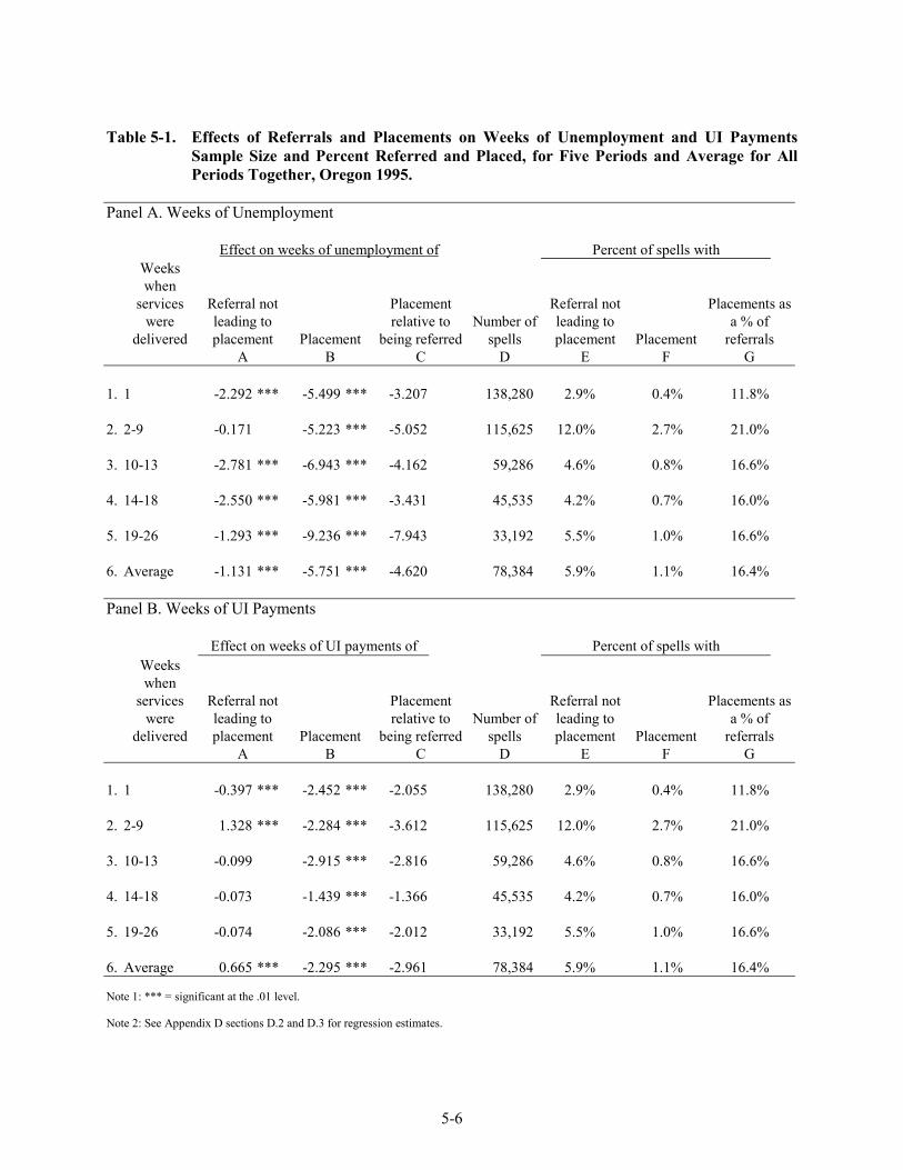
5-6
Table 5-1. Effects of Referrals and Placements on Weeks of Unemployment and UI PaymentsSample Size and Percent Referred and Placed, for Five Periods and Average for AllPeriods Together, Oregon 1995.
Panel A. Weeks of Unemployment
Effect on weeks of unemployment of Percent of spells withWeekswhen
serviceswere
delivered
Referral notleading toplacement Placement
Placementrelative to
being referredNumber of
spells
Referral notleading toplacement Placement
Placements asa % of
referralsA B C D E F G
1. 1 -2.292 *** -5.499 *** -3.207 138,280 2.9% 0.4% 11.8%
2. 2-9 -0.171 -5.223 *** -5.052 115,625 12.0% 2.7% 21.0%
3. 10-13 -2.781 *** -6.943 *** -4.162 59,286 4.6% 0.8% 16.6%
4. 14-18 -2.550 *** -5.981 *** -3.431 45,535 4.2% 0.7% 16.0%
5. 19-26 -1.293 *** -9.236 *** -7.943 33,192 5.5% 1.0% 16.6%
6. Average -1.131 *** -5.751 *** -4.620 78,384 5.9% 1.1% 16.4%
Panel B. Weeks of UI Payments
Effect on weeks of UI payments of Percent of spells withWeekswhen
serviceswere
delivered
Referral notleading toplacement Placement
Placementrelative to
being referredNumber of
spells
Referral notleading toplacement Placement
Placements asa % of
referralsA B C D E F G
1. 1 -0.397 *** -2.452 *** -2.055 138,280 2.9% 0.4% 11.8%
2. 2-9 1.328 *** -2.284 *** -3.612 115,625 12.0% 2.7% 21.0%
3. 10-13 -0.099 -2.915 *** -2.816 59,286 4.6% 0.8% 16.6%
4. 14-18 -0.073 -1.439 *** -1.366 45,535 4.2% 0.7% 16.0%
5. 19-26 -0.074 -2.086 *** -2.012 33,192 5.5% 1.0% 16.6%
6. Average 0.665 *** -2.295 *** -2.961 78,384 5.9% 1.1% 16.4%
Note 1: *** = significant at the .01 level.
Note 2: See Appendix D sections D.2 and D.3 for regression estimates.

5-7
In contrast, most Washington claimants helped by direct placement services would havebeen unemployed considerably longer than other claimants had they not received aid. Part of thedifference is that the Oregon results cover only 1995, while the Washington results apply to 1987-95,years that included a major recession and an extensive period where extended benefit programs wereactive.
There also are several possible additional reasons for these differences. Oregon may havegiven claimants incentives to search harder and more effectively for work over their entire spell ofunemployment than Washington by (a) enforcing the UI work test more stringently, (b) requiring mostclaimants to register in person with the PLXs, (c) making receipt of more PLX services mandatory, and(d) more readily providing additional voluntary supportive than Washington.
Panel B of Table 5-1 displays estimates of the reduction of weeks of UI payments.Placements are associated with a 2.3-week reduction in the number of weeks UI payments are made.However, referrals not leading to placements are associated with a 0.7 more weeks of payments. Thus,placements relative to viewing listings (rather than not receiving referrals) lead to a 3.0-week decrease inthe number of weeks with payments.
The small increase in payments due to referrals is primarily a result of a 1.3-week gain in theperiod including the second through ninth week of unemployment. About 55 percent of all referrals aremade in this period, and Oregon claimants might slightly delay taking new jobs in order to review listingsor comply with registration requirements. Alternatively, the small positive effect might be due tomeasurement error.
5.3 Estimating Total Benefits
To estimate total benefits, we need to multiply estimates of the per-incident effect ofreferrals and placements times the number of incidences. The administrative data provide estimates ofboth the per-incident effect and number of incidences. Chapters 3 and 4 detail why we believe that ourprocedures for estimating the effect of placements (relative to viewing listings and receiving staffassistance) are reasonably accurate, and why it is reasonable to use two alternative measures of the effectof viewing listings and receiving staff assistance relative to not receiving referrals (and usually notreceiving any PLX aid).

5-8
Chapter 4 also describes the procedures we used to ensure that the measure of incidence ofreferrals and placements is accurate. First, we compared the number of spells of unemployment in theWashington database for each year 1987 through 1995 to the number of first payments reported in officialUI statistics. Second, we compared the referral and placement rates across the years.
Our findings were that the Washington data were incomplete for the first 3 years and for thelast year. The problems with the early years were traced to not retaining all the data when the computersystems were updated. However, a deeper reason is that interest in creating longitudinal files for analysisfrom the administrative database did not begin until 1992. Thus, there was little reason to be concernedabout retention of the 1987-89 data beyond a 3-year period required to ensure UI claims were beingproperly made. In contrast, the data for the last year in the series were incomplete simply because the datawere not available for all of 1995 when the database was created.
Because the Washington files included data covering all unemployment spells, referrals, andplacements for the 1990-1994 period, we focused our estimates on this period and felt that it was notnecessary to estimate the incidence of these events for the other years. However, we only had estimates ofthe per-incident effects in Oregon for a single year, 1995. Thus, to accurately estimate total benefits it wasnecessary to determine if the incidence of unemployment, referrals, and placements was accuratelyreported in the administrative data, and if it was not accurate, use official statistics to produce accurateestimates.
The next subsection describes (a) how we used published statistics to estimate the actualincidence of unemployment, referrals, and placements in both Washington and Oregon for 1995; (b) howthese statistics compared to analogous figures derived from the person-level administrative files, and (c)how we used the Washington comparisons to adjust the Oregon figures to accurately measure theincidence of referrals and placements. We then used these figures to produce estimates of total benefits inthe following subsection.

5-9
5.3.1 Measuring the Incidence of Referrals and Placements
Table 5-2 displays key measures of PLX usage and services provided to claimants inWashington and Oregon covering 1995. Because the published data cover program years stretching fromJuly of 1 year to June of the next year, we averaged the figures for program years 1994 and 1995 to obtainmeasure covering calendar year 1995.1 Line 1 of panel A of Table 5-2 presents the total number of jobseekers registering with PLXs in each state. Line 2 displays the number of claimants who registered, andlines 3 and 4 display the number of claimants who were referred and placed, respectively. (In this casereferrals include those who were, and were not, placed.)
The key findings based on panel A are that the official statistics for Washington and Oregonare quite similar even though Oregon’s labor force is only 60 percent of the size of Washington’s. Theproportion of registrants who are claimants is slightly lower in Oregon than Washington. The proportionof claimants who are referred is slightly higher, and proportion of claimants who are placed, given theyare reviewed, also is slightly higher.
Panel B of Table 5-2 presents statistics on the number of unemployment spells, as well as thenumber of referrals and placements made to claimants recorded in the person-level administrativedatabases. The Washington and Oregon figures are for 1995, but the Washington figures had to beadjusted for the shortfall due to the data covering only a portion of that year. We multiplied the partial-year numbers by 1.67 to make the adjustment. This figure was used because we assumed that the ratio ofclaimants in the person-level file in 1994 to first payments observed in 1994 would also prevail in 1995.
The variables in panel B are not identical to those in panel A. Claimants who register withPLXs reported in panel A could be considerably less than the number of spells of unemployment because(a) not all claimants register with PLXs, and (b) some claimants have more than one spell ofunemployment in a calendar year.
1 The statistics for program years 94 and 95 were quite similar. Referrals and placements as a percent of claimants registered with PLXs were
almost identical. However, there were about 15 percent fewer claimants in program year 95 than 94. We, therefore, doubt that averaging thefigures for the 2 years has much, if any, affect on the comparisons.

5-10
Table 5-2. Claimants and Claimants Referred and Placed Measured with Published Statistics andTabulations of Person-level Files, Oregon and Washington 1995.
Panel A. Measures Derived from Published Statistics for Program Years 94 and 95
Oregon Washington Oregon
NumberPercent ofapplicants Number
Percent ofapplicants
Washington(col A / col C)
A B C D E1 Applicants 410,832 420,882 97.6%2 Claimants 200,897 48.9% 223,312 53.1% 90.0%
Percent ofClaimants
Percent ofClaimants
3 Referred 54,605 27.2% 54,517 24.4% 100.2%4 Placed 13,579 6.8% 11,524 5.2% 117.8%5 Placed/Referred 24.9% 21.1% 117.6%
Panel B. Measures Derived from Tabulations of Person-Level Files
Oregon Washington
NumberPercent of panel
A measures NumberPercent of panel
A measuresOregon/
WashingtonA B C D E
6 Claimants 132,280 65.8% 232,701 104.2% 56.8%7 Referrals 25,865 47.4% 34,648 63.6% 74.7%8 Placements 4,726 34.8% 7,533 65.4% 62.7%9 Placed/Referred 18.3% 21.7%
Panel C. Adjusted Oregon Measures
Oregon
NumberPercent ofapplicants
Adjustment factor(panel B col D /
col B)A B C
10 Claimants 209,344 104.2% 1.5811 Referrals 34,704 63.6% 1.3412 Placements 8,876 65.4% 1.8813 Placed/Referred 25.6%

5-11
Referrals and placements to claimants in panel A could be greater than those reported inpanel B because panel B only includes those made while benefits are being received within the first 26weeks of an unemployment spell. It is likely that many claimants use PLX services and accept jobs justafter benefit collection ends because either benefits are exhausted or claimants stop collecting to leavesome funds available for subsequent unemployment. On the other hand, the statistics in panel B allow formultiple referrals, while those in panel A are supposed to reflect the number of different people referred.
Because the statistics in the two panels are not identical, it is instructive to compare the twodifferent statistics for Washington where we are reasonably confident the database is complete. Thus,shortfalls in referrals and placements should reflect the effect of the restrictions imposed on the database,not an inherent difference in the population being observed. The Washington comparisons show that thenumber of spells is 4.2 percent greater than the number of claimants registering, suggesting that mostclaimants register with PLXs. However, both the number of referrals and the number of placements in thedatabase are only about 65 percent of those reported in official publications. This suggests that substantialuse of PLXs is made by claimants at or near the point benefits are exhausted and are, therefore, notincluded in our measures.
Panel B also shows that all the Oregon statistics in panel B are considerably less thananalogous statistics in panel A and, even more importantly, are considerably less than the same statisticsin panel B for Washington. We conclude from these comparisons that it is highly likely that the Oregonadministrative data do not cover all claimants and all PLX services provided to the claimants included.
In particular, it is hard to see how the number of spells of unemployment included inadministrative file could be smaller than the number of claimants registering with Oregon PLXs. Incontrast, the number of referrals and placements in panel B easily could be lower than the number inpanel A. However, the shortfalls should be proportional to those in Washington.
As noted earlier, the same pattern of shortfalls emerged in the first several years of theWashington administrative data used in Chapter 4. There were substantial shortfalls in the number ofspells of unemployment and even more substantial shortfalls in the number of referrals and placements.We, therefore, decided to adjust the Oregon figures so the proportion of spells, referrals, and placementsin the administrative files relative to those reported in official publications would be equal to those inWashington.

5-12
Column C of panel C in Table 5-2 shows the adjustment factors for each variable needed toequalize the proportions in Oregon with those in Washington. By far the largest adjustment, an 88 percentincrease, was made to the number of placements. The smallest adjustment, a 34 percent increase, wasmade to the number of referrals. This adjustment was smallest because the Washington data excludedmany cases where multiple referrals were made when ultimately the claimant was placed, but thisadjustment was not made with the Oregon data. As a result, the adjustments reduce a potential source ofoverestimation of the total benefits.
Finally, Table 5-3 displays some published statistics for 1998 that help explain why Oregon,whose labor force was only 60 percent of Washington’s, was able to refer and place about the samenumber of claimants as Washington. Unfortunately, we were unable to secure comparable data for 1995.However, we believe that they reflect differences that also prevailed in 1995.
First, lines 5 and 6 display the proportion of all referrals and all placements that were madeto claimants in the two states. In Washington, only about 25 percent of referrals and placements weremade to claimants, compared to about 38 percent in Oregon. Although both states have special programsto aid claimants, Oregon’s program has much greater funding in total and even greater funding perclaimant. Thus, far more of PLXs resources are targeted on claimants in Oregon than Washington.
Second, line 7 shows the number of job openings listed with PLXs. Despite Oregon havingonly about 60 percent of Washington employment, Oregon’s PLXs were able to secure about 4.3 percentmore openings. Clearly, the more openings that are available the more openings can be filled. However,line 11 shows that the proportion of openings filled was higher in Washington than Oregon. This seems tobe a natural outcome of Washington having more applicants per opening than Oregon in 1998. Line 12shows that the average wage of job openings listed with PLXs in Oregon were a bit higher than those inWashington. This, too, is evidence that Oregon PLXs were able to obtain a broader range of jobs thanWashington PLXs.
Most likely, Oregon PLXs were able to obtain a greater number and range of job ordersbecause they used some of their greater funding to put more effort into securing more listings.

5-13
Table 5-3. Selected Statistics Describing Direct Placement Services and Job Order Characteristicsin Washington and Oregon from July 1997 through June1998 and Labor ForceCharacteristics for 1990....
Oregon Washington
Oregon /Washington
(col A / col B)A B C
A. Referral and Placement CharacteristicsTotal Referrals1a. Number 197,848 171,299 115.5%1b. % of applicants 46.4% 26.3%
Total Placements2a. Number 44,098 46,182 95.5%2b. % of applicants 10.3% 7.1%
Claimant Referrals3a. Number 75,255 44,870 167.7%3b. % of claimant applicants 36.1% 10.8%
Claimant Placements4a. Number 17,342 11,144 155.6%4b. % of claimant applicants 8.3% 2.7%
38.0% 26.2%5. Percent of all referralsmade to claimants
39.3% 24.1%6. Percent of all placementsmade to claimants
B. Job Order Characteristics7. Openings 152,304 145,994 104.3%8. Orders 92,803 65,185 142.4%9. Openings per order 1.64 2.24
10. Openings filled 54,150 60,225 89.9%11. % of openings filled 35.6% 41.3%
12. Average wage of listings $8.89 $8.58 103.6%13. Average wage of placements $8.18 $8.56 95.6%
C. Labor Force Characteristics14. Population (millions) 2.854 4.888 58.4%15. Employment (millions) 1.327 2.275 58.3%16. Employment / Population 46.5% 46.5%

5-14
Although not shown in Table 5-3, the recall rate among claimants (not necessarilyregistrants) derived from the person-level files suggests that Oregon was able to place more claimantsbecause a lower proportion was recalled, and therefore, its claimants were considerably more likely toneed to find a new job.
5.3.2 Estimates of Total Benefits
In Table 5-4, the adjusted estimates of the number of referrals and placements in Oregonshown in Table 5-3 are multiplied by the per-incident effects of referrals and placements shown in Table5-1 to estimate the total reduction in the number weeks of unemployment resulting from direct placementservices.
Table 5-4 displays comparable results for Oregon and Washington using two differentestimates of the total effects. The estimates presented in columns A and C use incident estimates derivedfrom the person-level files. The estimates presented in columns B and D use incident estimates based onpublished statistics.
The Washington results shown in columns C and D use 1995 estimates of the number ofreferrals and placements, but 1994 estimates of the per-incident effects. The estimate of the effect ofplacements (relative to obtaining referrals) derived by subtracting the referral effect from the placementeffect is almost the same in 1994 and 1995. However, the 1995 referral effect is overestimated becausewe were unable to track the return to work over a sufficiently long period. That is why we use the 1994estimates.
Two different measures of the benefits also are presented. One only includes the effect ofplacements relative to obtaining a referral. These estimates are analogous to those described in Chapter 3and verified as accurate using a natural experiment. The other adds to the above estimate the benefitsfrom the “referral effect”-- the effect of obtaining a referral and staff assistance both on those referred butnot placed and those placed. The accuracy of the referral effect could not be verified using any type ofexperimental design. Thus, some of the positive effect could be due to self-selection or other forms ofmeasurement error.

5-15
Table 5-4. Estimates of Total Benefits Due to 1995 Referrals and Placements of Claimants inOregon and Washington
Oregonincidents based on
Washingtonincidents based on
Person-levelfile
Publishedstatistics
Person-levelfile
Publishedstatistics
A B C D1. Referral incidents 34,704 54,605 34,648 54,5172. Placement incidents 8,876 13,579 7,533 11,524
Reductions in weeks of unemployment:3. Per-referral 1.1 1.1 1.6 1.64. Per-placement 4.6 4.6 6.6 6.6
Total reduction in weeks of unemploymentdue to:
5. Referrals (line 1 x line 3) 38,175 60,066 55,437 87,2276. Placements (line 2 x line 4) 40,829 62,463 49,718 76,058
7. Average weekly earnings of claimants aided
$247 $247 $260 $260
Total earnings increase due to:8. Referrals (line 7 x line 5) $9,429,225 $14,836,302 $14,413,574 $22,679,0729. Placements (line 7 x line 6) $10,084,763 $15,428,361 $12,926,563 $19,775,18410. Total earnings increase due to
referrals and placements$19,513,988 $30,264,663 $27,340,137 $42,454,256
11. PLX Budget in 1995 $26,000,000 $26,000,000 $24,300,000 $24,300,000
Earnings increase as a percent of budget:
12. Due to placements 38.8% 51.0% 53.2% 81.4%13. Due to referrals and placements 75.1% 116.0% 112.5% 174.7%14. Percent of budget spent on claimants 38.0% 38.0% 25.0% 25.0%
Benefit-Cost Ratio15. Due to placements 1.02 1.56 1.26 2.1316. Due to referrals and placements 1.98 3.06 2.62 4.50
Notes: In this table the per-incident effect of referrals is relative to no referrals. Thus, the measure includes thepositive effects of obtaining information from viewing listings and receiving staff assistance that helps claimantsmore quickly find work on their own or accept jobs to which they were referred.
The per-incident effect of placements is measured relative to acquiring the information needed to obtain a referraland obtaining a referral that does not lead to a placement.
The incident of referrals include referrals not leading to placements and leading to placements. The percentage ofbudget spent on claimants (line 14) is based on the fraction of all referrals made to claimants.

5-16
Lines 1 and 2 of Table 5-4 show the number of referrals (both those leading and not leadingto placements) and number of placements. Lines 3 and 4 show the per-incident effect of referrals (relativeto no referrals) and placements (relative to being referred). Lines 5 and 6 show the total reduction inweeks of unemployment derived by multiplying the incidents times the per-incident effect.
In order to translate the total number of weeks into an increase in earnings, we multiply thenumbers on lines 5 and 6 by $247 for Oregon and $260 for Washington. The Washington earningsnumbers were derived by examining the post-unemployment earnings of referred and placed claimants.We did not have comparable data for Oregon, so we adjusted the Washington earnings using the ratio ofaverage hourly wages of placements in the two states.
Line 9 shows the increase in earnings due to placements (relative to being referred). This isthe lower bound estimate of the benefits. Line 10 shows the sum of the referral and placement effects.Line 11 shows the cost of running all PLXs in 1995, and lines 12 and 13 show the percentage of totalcosts covered by the benefits accruing to claimants alone with referral effects excluded and included,respectively.
In both Oregon and Washington, there are slightly greater total reductions in weeks ofunemployment due to referrals than due to placements. This is because the number of claimants referredis about five times greater than the number placed, but the per-incident effect of placements is only fourtimes the effect of referrals.
However, the total reduction in weeks of unemployment is about 45 percent greater inWashington than Oregon. This is the case because the number of incidents is about the same in bothstates, but the per-incident effect is about 45 percent greater in Washington.
Using the lower-bound estimate of total benefits for Oregon shows that the benefits accruingto claimants while they are collecting benefits up to the 26th week of their unemployment spell is equal to38.8 percent of total costs. However, published statistics suggest that only 65 percent of claimants’referrals and placements are included in the column A estimates.
If we use the published statistics to estimate the incidence of referrals and placements,benefits going to claimants, the lower-bound estimate of claimant benefits increases to 51.0 percent of

5-17
costs. This is substantially greater than the estimate presented in Table 5-3 that 38 percent of the costs ofPLX services go to helping claimants.2
Naturally, if we include the referral effect the benefits even further exceed the portion of allPLX costs estimated to go toward claimants. Indeed, the estimate of total effects in column B, whichincludes the total number of placements is over 4 million dollars more than the cost of running the entirePLX.
While the Oregon results are quite impressive, the Washington results are even larger. Theminimum estimate suggests that benefits derived from placements to claimants cover twice the cost ofthis activity, while the maximum estimates suggest that the total benefits going to claimants is about 75percent greater than the entire cost of running the Washington PLXs.
5.3.3 Why Total Benefits Differ between Oregon and Washington
It would be of great value to improving the performance of PLXs to know why the resultsdiffer between Oregon and Washington. Unfortunately, at this time we can only speculate on why thedifferences exist, but their existence suggests that it would be highly fruitful to examine the followingplausible hypotheses:
1. Oregon has implemented procedures that make it more likely that claimants willintensively search for new jobs, or if they are not willing and able to searchintensively, they stop collecting benefits.
2. Oregon has used its resources to attempt to directly aid a far larger fraction ofclaimants. As a result, a higher proportion of claimants who are likely to return towork on their own receive services.
3. The characteristics of Oregon’s workers and/or labor markets are such that claimants,in general, are more likely to find work on their own.
The first hypothesis suggests that the comparison group has been strongly affected bypolicies implemented by its PLX and UI systems that give claimants incentives to assiduously search for
2 If we assume that the placement effects for claimants after they stop collecting benefits equals the effect observed for period 5 covering weeks
19 through 26, the average reduction for the 35 percent of claimants omitted from our sample would be 7.9 weeks, not the 4.6 weeks shown inTable 5-1. Thus, not using separate estimates for the omitted groups very likely leads to the estimates in column B and D being even moreconservative than those in columns A and C.
5-18
work or end benefit collection. If this is the case, the policies lower the value of direct placement servicesrelative to those in Washington. However, a fuller analysis of the benefits and costs of PLX activitieswould indicate that a lot of benefits of these activities are omitted from this analysis. Thus, the totalbenefits of all PLX (and UI) system activities could be far greater in Oregon than Washington.
The second hypothesis was mentioned in Section 5.3.1 as a possible explanation for why theper-incident effects are lower in Oregon than Washington. Pursuing this hypothesis could be of particularvalue, since it suggests that the same benefits could be attained by improving the targeting of services toclaimants. If additional analysis could identify groups of claimants whose benefits from direct placementservices do not cover the costs, it would be possible to raise the total benefits by providing less services tothose groups. For example, instead of requiring all claimants to register in person and review listings, itmight be possible to limit this requirement to those claimants most likely to be affected by this policy.
The third hypothesis suggests that factors outside the control of PLX and UI policies accountfor the differences. While there are some substantial differences in the characteristics of claimants in thetwo states, it is likely that most of these differences have been taken into account in producing theestimates.
The best way to test all three hypotheses would be to combine the databases for both states,add variables that better reflect policy differences in availability of services and mandatory requirementsto take certain action, and then reestimate the effects taking those differences into account. Use of cross-state differences is particularly important because it is very difficult to use data from one state alone toassess the effect of policies uniformly applied to claimants in that one state.
Because of Oregon’s more stringent confidentiality restrictions, we could not carry out thisanalysis at Westat as part of this study. However, we hope to do so as part of on-going work bytransferring the Washington data to the Oregon Employment Department.

5-19
5.4 Summary and Conclusions
The Oregon study addressed two questions:
Could a state employment security agency replicate the Washington analysis wecarried out using its own staff and computers with modest help from us?
Are the results for a second state as large as those for Washington?
We determined that the answer to the first question is definitely yes. However, any stateattempting to develop the person-level database needed to replicate the analysis should recognize that thisis a very demanding task that requires exceptional attention to detail. Also, any state should assume that itis likely to take several years before it can be certain that the following two goals are achieved:
1. The variables required for analysis are properly created.
2. The data coverage of the population is complete.
To reach goal 1, it is essential to directly compare the input and output files at each stage inthe data preparation process. A key suggestion is to structure the data preparation work assuming thatsome problem will be spotted with each person’s work longer after that person is not available forconsultation and would have forgotten the details of work. In short, it is imperative to createdocumentation that would allow an independent review of each person’s work, without any additional aidfrom that person.
To reach goal 2, it is essential to compare published statistics to analogous statistics derivedfrom tabulations of the person-level files at the outset and all through the data preparation processing. Wecannot explain why person-level data that once were used to produce aggregate statistics cannot easily bereassembled, but this has been our experience with every state where we have tried to perform this task.Also, we have found it to be difficult, if not impossible, to find missing data. However, once it becomesclear that the person-level files will be used for research, arrangements can be made to properly preservecurrent files.
Thus, one especially clear-cut conclusion is that the sooner a state starts to assemble person-level files for research purposes, the sooner problems with available data will be spotted, and the soonerthose problems can be resolved.

5-20
With respect to the second question regarding the relative size of the effect, it appears thatthe benefits of direct placement services are smaller both per-incident and in total in Oregon than inWashington. Placements relative to obtaining a referral and staff reduce unemployment by 4.6 weeks inOregon, compared to 6.6 weeks in Washington. The lower-bound estimate for the total benefits is $10million in Oregon, compared to $12.9 million in Washington. Moreover, we estimate that both statesspend about the same amount on their PLXs, but Oregon spends about 38 percent of the total PLX budgetto aid claimants, compared to Washington’s 25 percent.
In Oregon, all four estimates of benefits more than cover the costs of providing services toclaimants. The largest estimate suggest that benefits going to claimants more than cover the costs ofrunning the entire PLX.
In Washington, all four estimates far exceed the estimate of costs of providing services toclaimants. The lowest estimate suggests benefits are twice the costs to serve claimants, and highestsuggests benefits going to claimants are 75 percent greater than the cost of running the entire PLX.
Importantly, the estimates of the benefits of direct placement services in Oregon could beconsiderably lower than benefits in Washington because Oregon has implemented other policies thatdramatically reduce the time claimants who are not directly helped by PLXs remain unemployed. Thus,because those benefits are outside of this study, the full value of public services provided to claimants isdramatically underestimated.
However, even if this is the case, Oregon might be able to dramatically increase benefits ofdirect placement services by improving their targeting. We suspect that the benefits in Washington areparticularly high because many claimants voluntarily seek help usually long after most claimants havealready become reemployed. In contrast, Oregon benefits might be relatively low because claimants areencouraged (or required) to obtain aid far closer to the start of the unemployment spell. Thus, additionalanalysis might suggest ways to reduce the amount of services received by claimants who are likely toreturn to work quickly on their own.
We hope to be able to continue our work with the OED to answer the highly provocativequestions that are unresolved in this, our initial collaboration.

Chapter 6

6-1
6. CROWDING-OUT EFFECTS OF THE PUBLIC LABOR EXCHANGEIN WASHINGTON STATE1
6.1 Introduction
Improvements in public labor exchanges (PLXs) are intended to reduce the duration ofunemployment for jobless workers by improving the information available to those workers and byincreasing the rate at which they receive job offers. Improvements in the PLXs can be thought of asenhancements to the technology of job search that lead to increases in the rate at which jobless workersbecome reemployed. However, a potential unintended consequence of increasing the reemployment rateof one group of workers (in this case, users of the PLXs) is that the job prospects of other groups ofworkers may worsen. The reason is that improvements in the technology of job search for one group ofworkers may have the indirect effect of “crowding out” other groups of workers. For example, if thesearch technology available to PLXs registrants is better than the search technology available to otherworkers, then PLX registrants may beat other workers to job vacancies and fill those vacancies. As aresult, job vacancies that would normally be available to other workers are no longer available, and theother workers don’t receive job offers that they would otherwise receive. This crowding-out effect couldoffset part (or all) of the benefits of improving the services provided by the PLXs.
To investigate the crowding-out effects of the PLXs, we build on previous work on thecrowding-out effects of reemployment bonus programs and wage subsidies (Davidson and Woodbury1993, 1996). In particular, we develop and apply an equilibrium search and matching model of the labormarket in which heterogeneous unemployed workers are assumed to search randomly across firms for avacancy, and firms with vacancies randomly select workers from the pool of applications they receive.Each unemployed worker chooses a search effort (the number of firms to contact) in an effort tomaximize expected lifetime utility. Increasing search efforts raises the probability of reemployment but isalso costly. We characterize the steady-state equilibrium generated by the market in such an environmentand then examine how that equilibrium would change in the absence of the referral and placementactivities of PLXs. Comparing the two equilibria provides insight into the impacts of the PLXs on labormarket outcomes.
1 This chapter was written by Drs. Carl Davidson and Stephen A. Woodbury at Michigan State University.

6-2
In Section 6.2, we develop a general equilibrium model in which different groups of workersflow through different labor market states (employment and unemployment). The rates of transitionbetween different labor market states depend, in part, on the search technology available to workers, andthe model allows for interactions between different groups of workers. Section 6.3 describes how themodel is calibrated using labor market data from Washington State and recent evidence on the impacts ofPLXs in Washington State that have been produced by Westat, Inc. (Jacobson 1999). Calibrating themodel grounds the model in observed behavioral effects and, as much as possible, forces the model tolook like the actual labor markets that are of interest. We then solve the model without the PLXs andcompare the two solutions to obtain simulated impacts of the PLXs on workers who do not use the PLXs.
Section 6.4 describes the results of the simulations. In the model, the referral and placementactivities of the PLXs have two main effects. The first is a gross employment effect – that is, the PLXsreduce unemployment and increases employment of PLX users (workers who are referred or placed bythe PLXs). The second is the crowding-out effect, which occurs if some (or all) of the improvementexperienced by PLXs users comes at the expense of workers who do not use PLXs (workers who are notreferred or placed by PLXs). The simulations suggest that PLXs increase the overall level of employmentin Washington State and reduce the unemployment rate by a small amount (0.08 percentage points). Thesimulations also suggest a small crowding-out effect of PLXs: nonusers of PLXs experienceunemployment spells that are longer by 0.061 week (or 0.4 percent) as a result of the referral andplacement activities of PLXs. The net result of these two effects is that about one-quarter of theimprovement in labor market outcomes for which PLXs are responsible is offset by crowding out of PLXnonusers. It follows that the crowding-out effects of PLX referral and placement activities are small inrelation to the benefits.
6.2 Description of the Model
6.2.1 Overview
To examine the extent to which users of the PLXs might crowd out other workers, weemploy a model of the labor market in which workers must search for reemployment after losing theirjobs. The basic setup of the model is patterned after the labor market for workers covered by the

6-3
Unemployment Insurance (UI) program in Washington State during 1987 through 1995. In the model,there are three classes of workers:
UI claimants who are neither referred nor placed by PLXs, although they may beregistered with the PLXs (we refer to these as PLX nonusers);
UI claimants who are referred to at least one job opening by PLXs but are not placed;and
UI claimants who are referred and placed by PLXs.
In what follows, the subscript j can take three values: 0 always refers to the group ofnonusers; the subscript 1 always refers to those referred but not placed; and the subscript 2 refers to thosereferred and placed by the service.
Note that workers who do not claim UI benefits are not considered in this model. Inprinciple, they could be included. However, the data available for this study (see Jacobson 1999 andTable 6-1) are specific to UI claimants only. Although we focus on UI claimants in this chapter, weconjecture that including nonclaimants would not materially change the basic findings. We find that thereferral and placement activities of PLXs result in little crowding out of PLX nonusers by PLX users.Adding nonclaimants to the model would diffuse the small crowding-out effects over more workers andwould result in even smaller losses per PLX nonuser.
While unemployed, workers of type j (j = 0, 1, and 2) collect unemployment benefits (xj) andsearch for reemployment with search effort (pj) chosen to maximize expected lifetime income (VUj). Ineach period, the worker’s probability of reemployment (or match rate, mj) depends on his or her ownsearch effort (pj), the search effort of all other unemployed workers, and the vacancy rate. Since theprobability of reemployment is assumed constant throughout the spell of unemployment, the expectedduration of unemployment for a worker of type j is (1/mj) periods.
While employed, each worker of type j is paid a wage (wj) that is negotiated at the time ofinitial employment. In addition, in each period, each employed worker faces a risk of losing his or herjob; the probability of job separation is denoted by s. This implies that the expected duration of a job is(1/s) periods. Thus, workers cycle between employment and unemployment with each job lasting (onaverage) 1/s periods and each spell of unemployment lasting (on average) 1/mj periods.
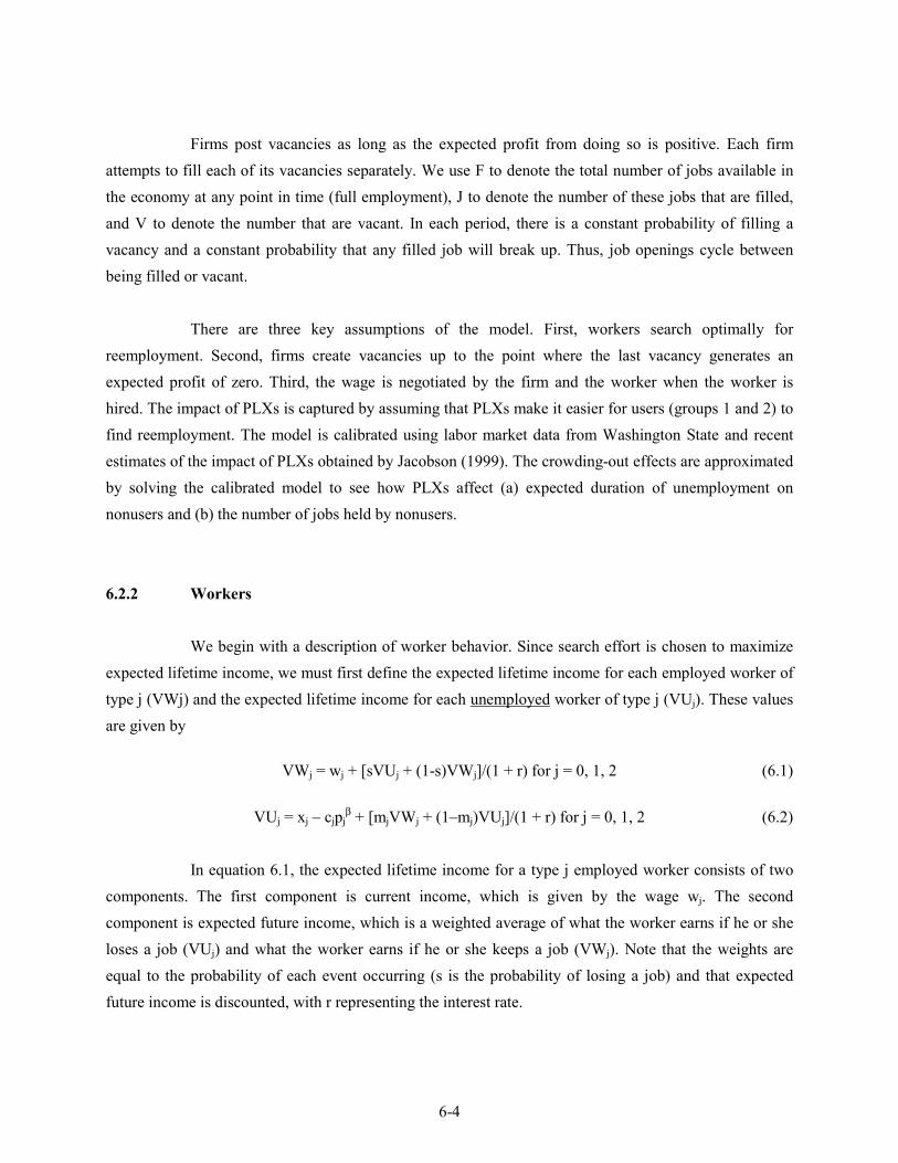
6-4
Firms post vacancies as long as the expected profit from doing so is positive. Each firmattempts to fill each of its vacancies separately. We use F to denote the total number of jobs available inthe economy at any point in time (full employment), J to denote the number of these jobs that are filled,and V to denote the number that are vacant. In each period, there is a constant probability of filling avacancy and a constant probability that any filled job will break up. Thus, job openings cycle betweenbeing filled or vacant.
There are three key assumptions of the model. First, workers search optimally forreemployment. Second, firms create vacancies up to the point where the last vacancy generates anexpected profit of zero. Third, the wage is negotiated by the firm and the worker when the worker ishired. The impact of PLXs is captured by assuming that PLXs make it easier for users (groups 1 and 2) tofind reemployment. The model is calibrated using labor market data from Washington State and recentestimates of the impact of PLXs obtained by Jacobson (1999). The crowding-out effects are approximatedby solving the calibrated model to see how PLXs affect (a) expected duration of unemployment onnonusers and (b) the number of jobs held by nonusers.
6.2.2 Workers
We begin with a description of worker behavior. Since search effort is chosen to maximizeexpected lifetime income, we must first define the expected lifetime income for each employed worker oftype j (VWj) and the expected lifetime income for each unemployed worker of type j (VUj). These valuesare given by
VWj = wj + [sVUj + (1-s)VWj]/(1 + r) for j = 0, 1, 2 (6.1)
VUj = xj – cjpjβ + [mjVWj + (1–mj)VUj]/(1 + r) for j = 0, 1, 2 (6.2)
In equation 6.1, the expected lifetime income for a type j employed worker consists of twocomponents. The first component is current income, which is given by the wage wj. The secondcomponent is expected future income, which is a weighted average of what the worker earns if he or sheloses a job (VUj) and what the worker earns if he or she keeps a job (VWj). Note that the weights areequal to the probability of each event occurring (s is the probability of losing a job) and that expectedfuture income is discounted, with r representing the interest rate.
6-5
In equation 6.2, the expected lifetime income for a type j unemployed worker consists of twocomponents. The first component is current income, which is given by unemployment benefits (xj) lesssearch costs (cjpj
β). [Recall that pj denotes the worker’s search effort. Additional search effort is assumedto reduce a worker’s income at an increasing rate, so pj is raised to the power β (>1), which is theelasticity of search cost with respect to search effort (search costs are convex in search effort). The termpj
β is then scaled by the multiplicative factor cj, which we refer to as the search cost parameter.]
The second component of expected lifetime income is expected future income, which is aweighted average of what the worker earns if he or she finds a job (VWj) and what the worker earns if heor she remains unemployed (VUj). Once again, the weights are equal to the probability of each eventoccurring (the probability of finding a job is mj) and expected future income is discounted.
Each unemployed worker chooses search effort to maximize expected lifetime income. Thus,for each worker pj is chosen to maximize equation 6.2; or
pj = arg max VUj for j = 0, 1, 2 (6.3)
Equations 6.1, 6.2, and 6.3 define optimal search effort. Our next goal is to show how searcheffort determines the reemployment probabilities. For each worker, we interpret search effort as thenumber of firms contacted in an effort to find a job. Once the worker contacts a firm, the probability ofgetting a job depends on (a) whether the job is vacant and (b) if the job is vacant, being chosen over allother job applicants. Since there are V vacancies and F total job openings, the probability that any givenopening is vacant at any point in time is V/F. In Davidson and Woodbury (1993), we showed that in thistype of model the probability that any given worker will be chosen over all other applicants to fill avacancy is given by (1/λ)[1 – e-λ] where λ is the total number of job applicants per job opening. Thus,equation 6.4 shows how search effort can be used to determine the reemployment probabilities
mj = pj(V/F)(1/λ)[1 – e-λ] for j = 0, 1, 2 (6.4)
where
λ = (p0U0 + p1U1 + p2U2)/F (6.5)

6-6
In equation 6.5, Uj is the number of type j workers who are unemployed in equilibrium, andF denotes the total number of job openings (filled and vacant).
6.2.3 Discussion
At this point, it is useful to summarize the model with the aid of Figure 6-1, which shows thestocks of each type of unemployed worker (U0, U1, and U2) and their flows through the labor market andinto jobs. In each period, we assume that unemployed workers choose search effort (pj) to maximizeexpected lifetime income. The optimal level of search effort for each type j worker is defined byequations 6.1, 6.2, and 6.3. These workers then compete with each other for the jobs that are available inthe labor market. The levels of search effort determine the number of applications filed at each firm, andeach firm is assumed to choose randomly from the pool of applicants to fill vacancies. With theseassumptions, equations 6.4 and 6.5 show how the levels of search effort can be translated intoreemployment probabilities (mj) for each type of worker. These reemployment probabilities thendetermine the number of type j job seekers who find new jobs each period.
6.2.4 Firms
We assume that firms create vacancies as long as the expected profit from doing so is non-negative. Let πv denote the expected lifetime profit for a firm with a vacancy and let πj denote theexpected lifetime profit for a firm with a job opening that is filled by a type j worker. Furthermore, let qj
denote the per period probability of filling a vacancy with a type j worker and let Rj denote the per periodrevenue generated by a type j worker. Then πv and πj are given by
πv = -K + [q0π0 + q1π1 + q2π2 + (1-q0-q1-q2) πv]/(1 + r) (6.6)
In equation 6.6, K represents the cost of maintaining the job opening when it is vacant. Notethat πv consists of two components. The first component, -K, is the current period profit associated withhaving a vacancy. The second component measures expected future profit, which is the weighted averageof the profit earned by filling the vacancy with a worker of each type. The weights are the probabilities offilling the vacancy with each type of worker, and this second component is discounted at the interest rateto take into account that it is earned in the future.

6-7
U0 U1U2
Labor Market
p0U0 p1U1 p2U2
J0J1 J2
m0U0m1U1
m2U2
Figure 6-1. The labor market
The expected lifetime profit for a firm with a job opening filled with a type j worker (πj) iscalculated in a similar manner. The first term on the right-hand side of equation 6.7 captures currentprofit, which is revenue (Rj) net of the wage (wj). The second term captures expected future profit, whichis the weighted average of (a) what the firm can expect to earn in the future if the job lasts another periodand (b) what the firm can expect to earn in the future if the job breaks up at the end of the current period.
πj = Rj – wj + [sπv + (1-s) πj]/(1 + r) for j = 0, 1, 2 (6.7)
Since we have assumed that firms create vacancies until the expected profit earned by thefirm creating the last vacancy is zero, we know that in equilibrium
πv = 0 (6.8)
We complete our description of firm behavior by explaining how the equilibrium wages aredetermined for each type of worker. We assume that once the firm and worker meet, they negotiate thewage by making offers and counteroffers until an agreement is reached. As is well known by now, such

6-8
negotiations lead to an outcome that is described by the Nash Cooperative Bargaining Solution, whichsplits the surplus generated by the job evenly between the firm and worker. For a worker of type j, thesurplus created by the job is VWj – VUj since this measures the increase in expected lifetime income fromaccepting the job. For the firm, the surplus created by the job is πj - πv since this measures the increase inexpected lifetime profits from filling the vacancy with a type j worker. Thus, if wj splits the surplusgenerated by the job evenly, it must satisfy
πj - πv = VWj - VUj for j = 0, 1, 2 (6.9)
6.2.5 Equilibrium
We begin our description of equilibrium by introducing some accounting identities thatallow us to keep track of employment, unemployment, and their composition. In each period, a workermust either be employed or unemployed. Thus, if we let Lj denote the total number of type j workers inthe economy and use Jj and Uj to denote the number that are employed and unemployed, respectively,then we must have
Lj = Jj + Uj for j = 0, 1, 2 (6.10)
We use J to denote total employment and U to denote total unemployment. It follows that
J = J0 + J1 + J2 (6.11)
U = U0 + U1 + U2 (6.12)
Finally, each job opening must be either filled or vacant. Thus, we must also have
F = J + V (6.13)
where F denotes the total number of job openings and V denotes the total number of vacancies.
In equilibrium, the flow into each state of employment must equal the flow out of that state.For example, in each period mjUj unemployed type j workers find new jobs. It follows that mjUj is theflow into state Jj. At the same time, sJj type j employed workers lose their jobs. Thus, sJj is the flow out of

6-9
state Jj. In equilibrium, these flows must be equal so that employment of type j workers remains constant.Therefore, it is necessary that
mjUj = sJj for j = 0, 1, 2 (6.14)
The employment dynamics for each type of worker are depicted in Figure 6-2, which showsthe flows of workers into and out of each labor market state. Equation 6.14 guarantees that these flowswill be equal so that the employment and unemployment levels for each type of worker will not changeover time in equilibrium.
Uj Jj
mjUj
sJj
Figure 6-2. Employment dynamics for type j workers
A final equilibrium condition allows us to calculate the firm’s probability of filling itsvacancy with a type j worker (qj). Since each job consists of one worker and one vacancy, the number ofvacancies filled by a type j worker in each period (qjV) must equal the total number of type j workers whofind employment in that period (mjUj). Thus, we must have
qjV = mjUj for j = 0, 1, 2 (6.15)
Equations 6.14 and 6.15 together imply that the number of firms and vacancies will remainconstant over time.
This completes the description of the model. The key parameters of the model are s (theseparation rate), r (the interest rate), cj and β (the search cost parameter and the elasticity of search costwith respect to search effort), xj (unemployment benefits), Rj (the revenue generated by a type j worker),K (the cost of maintaining each vacancy), and Lj (the number of type j workers in the economy). Theendogenous variables are VWj, VUj, pj, mj, λ, wj, πv, πj, F, Jj, Uj, J, U, V, and qj. Note that the modelconsists of 33 equations in 33 unknowns. There are 16 parameters.

6-10
6.2.6 Why Use an Equilibrium Search and Matching Model?
Before explaining how the model can be used to estimate the displacement effect of PLXs, itis useful to discuss why we have chosen to work with such a model. If there were full employment,displacement would not be an issue—each worker who wanted to work would be able to find a job andthere would be no concern about one worker displacing another. Of course, in an economy of fullemployment, programs such as the PLX would not be necessary because every worker would be able tofind a job without government assistance.
However, full employment does not prevail, even in the current period of prosperity.Standard economic models have often been criticized for assuming full employment, and economists haveworked hard to replace the standard textbook models of supply and demand with more realistic models ofthe labor of the labor market. In these models, the informational asymmetries and transaction costs (ortrade frictions) that keep the market from clearing are taken into account so that there is an “equilibrium”rate of unemployment. The search model used in this report follows in this tradition. It emphasizes thetime and effort needed for unemployed workers and firms with vacancies to find each other. These tradefrictions result in an equilibrium rate of unemployment and provide some justification for governmentintervention aimed at either lowering unemployment or reducing the time it takes for unemployedworkers to find new jobs. Accordingly, the search framework provides an ideal setting for investigatingthe impact of government programs such as PLXs.
Three additional features of the model make it particularly useful for estimating thecrowding-out effects of PLXs. First, the key parameters of the search model are the turnover rates; that is,the separation rate and the reemployment probabilities. Research exists that suggests values of separationrate. The duration of unemployment, which is linked directly to the reemployment probability, can beobserved directly. As a result, the model can be calibrated using existing data. (This is discussed further inthe next section.) Once calibrated, the model looks remarkably similar to the actual labor market inWashington State.
Second, the key parameters of the model can be altered to simulate different types of labormarkets. For example, when the separation rate is increased, the model’s equilibrium rate ofunemployment rises. Thus, by increasing the separation rate and examining the impact of this parameterchange on crowding out, we can gauge the impact of a program such as the PLXs at different stages in thebusiness cycle.

6-11
Finally, by modeling job search explicitly, we are able to show how PLXs directly affect theproblem faced by unemployed workers. For those who use PLXs, the cost of contacting a given numberof firms is lowered. In terms of the model, for users, PLXs lower cj, the cost-of-search parameter. Fornonusers, PLXs make it harder to find employment because λ, the average number of applications filedper firm, rises while the number of contacts they make does not change. Since users are contacting morefirms, the reemployment probability for all nonusers falls. (In terms of the model, m0 falls if p0 remainsconstant while λ increases.)
6.3 Implementing the Model
Several of the key parameters of the model are observable. For example, we know that inWashington State there were roughly 282,000 UI claimants who were neither referred nor placed byPLXs during the period in question. In addition, roughly 34,000 UI claimants were referred but not placedby PLXs, and roughly 12,600 UI claimants were referred and placed by PLXs. Thus, we measure workersin thousands and set L0 = 282, L1 = 34 and L2 = 12.6. We also have data on the unemployment benefitscollected by these workers, the wages they earned, and their average durations of unemployment (DUj).Measuring time in weeks, we have w0 = 365, w1 = 304, w2 = 252, x0 = 188, x1 = 181, x2 = 158, DU0 =13.9, DU1 = 17.9 and DU2 = 12.3. These data are summarized in Table 6-1. Although the wages andexpected durations of unemployment are not parameters of the model, we use these values to infer someof the underlying parameters that cannot be observed.
For the separation rate, we turn to the literature on labor market turnover. Estimates of thisparameter can be found in Clark and Summers (1982), Ehrenberg (1980), and Murphy and Topel (1987).We set s = .005 in our reference case and then vary s to make sure that our results are not sensitive to thisassumption. For the interest rate, we set r = .004. We know from previous work with models similar tothis one that the results are largely insensitive to changes in the assumed value of r.

6-12
Table 6-1. Descriptive Statistics of Public Labor Exchange (PLXs) Registrants, and EstimatedImpacts of the PLXs, Washington State, 1987-1995
All NonusersReferred/not placed
Referred/placed
Weekly wage beforeunemployment ($) 355 365 304 252Weekly UI benefit amount ($) 186 188 181 158UI replacement rate 0.52 0.52 0.60 0.63Spell duration (weeks)
Insured unemployment 14.3 13.9 17.9 12.3Total unemployment 20.6 20.7 23.2 13.1
PLXs impact (weeks)Insured unemployment -- -- -0.56 -4.25Total unemployment -- -- -2.43 -12.59
Number of individuals 328,815 282,240 33,990 12,585
Source: Jacobson (1999).Note: PLXs nonusers are PLXs registrants who are neither referred nor placed by PLXs.
The search cost parameters are the next consideration. In Davidson and Woodbury (1996),we calibrated a variation of this model for Washington State in an effort to explain the results of theWashington Reemployment Bonus experiment, which was conducted during 1988-1989 (Spiegelman,O’Leary, and Kline 1992). We found that in order to explain the effects that were observed in the bonusexperiment, β would have to be between 1.5 and 1.7. Thus for the reference case we set β = 1.6, but wesolve the model and obtain estimates of crowding out for β = 1.5 and 1.7 as well.
Finally, solving the model requires values of cj, Rj, and K. To obtain estimates of thesevalues, we use the data on wages and average durations of unemployment mentioned above. We also addone other equation to the model. From Abraham (1983), we know that the number of job vacancies perunemployed workers (V/U) is typically close to 1/2 (that is, there is usually one job vacancy for every 2unemployed workers), although that ratio varies between 1/3 and 1 over the business cycle. If we add thisequation to the model and set wj and DUj equal to the values above, we can solve the model for themissing parameters (cj, Rj and K). This gives us values of the parameters that make the model consistentwith Jacobson’s (1999) estimates of the impact of PLXs in Washington State.
Once the model is calibrated, we are in position to estimate the crowding-out effects ofEmployment Service referrals and placements. Jacobson (1999) estimates that a PLX referral reduces theaverage duration of unemployment by .56 weeks and that a referral leading to a placement reduces the
6-13
average duration of unemployment by 4.25 weeks. In the model, the activities of PLXs (that is, referralsand placements) change the search cost parameters (c1 and c2) by making it easier (or less costly) forworkers who receive a referral to make job contacts. Thus, we re-solve the model for the new values of c1
and c2 that make the model’s results consistent with Jacobson’s estimated impacts of PLX referrals andplacements in Washington State. The model’s solution yields estimates of J0 and m0 (the number of jobsand the probability of reemployment for PLX nonusers) that allow us to measure the impact of PLXreferrals and placements on the employment level and average unemployment duration of workers whodo not receive PLX referrals (the nonusers).
To summarize, we start with a model that has 33 equations in 33 unknowns and 16parameters. We obtain estimates of the parameters needed to implement the model from various sources:the separation rate and the interest rate come from the published literature; unemployment benefits comefrom Jacobson’s study of PLXs in Washington State (Jacobson 1999); and the elasticity of search costswith respect to search effort (β) is taken from our previous work (Davidson and Woodbury 1993, 1996).
However, several parameters cannot be observed: the search cost parameters (c0, c1, and c2);the revenue generated by each type of worker (R0, R2, and R2); and the cost of maintaining a vacancy (K).We use data from Jacobson (1999) to infer values for these missing parameters. We do so in two steps.First, we take values for six of the endogenous variables (wages - w0, w1, w2 - and the average duration ofunemployment - DU0, DU1, DU2) from Jacobson (1999) and take an estimate of U/V from the literature(Abraham 1983). Adding these seven values to the model allows us to solve for the seven missingparameters and gives us a model that is then consistent with the data and findings in Jacobson (1999).
The second step is to infer how the program alters the cost of search for each group of users.We do this by using Jacobson’s estimate of the impact of PLXs on the average unemployment durationsof PLXs users. Accordingly, we re-solve the model with all of the parameters held fixed (including thevalues for c0, R0, R2, R2 and K that were solved for in stage 1). This yields values of c1 and c2 that wouldlead to the reductions in DU1 and DU2 that were observed in Jacobson’s study. In other words, we modelthe program by assuming that PLXs cause c1 and c2 to fall, and then we check to see how much they mustfall to completely explain the observed outcome.

6-14
6.4 Results
In the model described in the previous section, the referral and placement activities of PLXshave two main effects. First, they improve the labor market outcomes of PLX users, reducing theirunemployment durations and increasing their employment. This can be thought of as a gross employmenteffect of PLXs. Second, some (or possibly all) of the improvement experienced by PLX users may comeat the expense of workers who do not use PLXs. This is the crowding-out effect that motivates this report.The simulations address the following questions. How large is the displacement effect in relation to thegross employment effect of PLXs? Does the gross employment effect outweigh the displacement effector, alternatively, is there a one-for-one trade-off between improvements for PLX users and crowding outof nonusers? Do PLX referral and placement activities lead to an increase in overall steady-stateemployment (and a decrease in overall unemployment)?
Tables 6-2 and 6-3 display results of the simulations. Table 6-2 shows the results of ninesimulations using three different values of the separation rate (s = .004, .005, and .006) and three differentvalues of the elasticity of search cost with respect to search effort (β = 1.5, 1.6, and 1.7). Table 6-3 showsthe results of another nine simulations using the same three values of the separation rate (s = .004, .005,and .006) but this time varying the value of the number of vacancies to unemployed workers (V/U = 1/3,1/2, and 1). Varying the ratio of vacancies to unemployed workers is a way to checking how thecrowding-out effects of the PLXs might vary over the business cycle.
6.4.1 Reference Case
Consider first the reference case, which is in the middle column of Table 6-2. The referencecase uses parameter values that we believe to be the most likely to obtain in fact: a separation rate (orweekly probability of separating from a job) of .005, an elasticity of search cost with respect to searcheffort (β) of 1.6, and two unemployed workers for every job vacancy (V/U = 1/2).

6-15
Table 6-2. Simulated Impacts of PLXs on Unemployment Duration, Employment, and the TotalUnemployment Rate, Washington State, for Various Separation rates (s) andElasticities of Search Effort (ββββ)
Separation rate (s): 0.004 0.005 0.006Elasticity of search effort (β): 1.5 1.6 1.7 1.5 1.6 1.7 1.5 1.6 1.7Change in unemploymentduration (in weeks) ofworkers:
who do not use PLXs .141 .059 .073 .003 .061 .062 .061 .061 .061referred by PLXs -0.56 -0.56 -0.56 -0.56 -0.56 -0.56 -0.56 -0.56 -0.56placed by PLXs -4.25 -4.25 -4.25 -4.25 -4.25 -4.25 -4.25 -4.25 -4.25
Change in employmentof workers:
who do not use PLXs -147 -61 -76 -3 -76 -76 -88 -88 -88referred by PLXs 66 66 66 80 80 80 93 93 93placed by PLXs 191 191 191 233 233 233 272 272 272
Change in total employment 110 196 181 310 237 237 277 277 277Change in total
Unemployment rate -.04 -.06 -.06 -.09 -.07 -.07 -.09 -.09 -.09Notes: Vacancies per unemployed worker (V/U) are set to 1/2 in all the above simulations. Other parameters of the model are set to the valueslisted in the text. PLXs nonusers are PLXs registrants who are neither referred nor placed by PLXs. See the results section for discussion.
Table 6-3. Simulated Impacts of PLXs on Unemployment Duration, Employment, and the TotalUnemployment Rate, Washington State for Various Separation Rates (s) and Vacanciesper Unemployed Worker (V/U)
Separation rate (s): 0.004 0.005 0.006Vacancies per unemployedworker (V/U): 1/3 1/2 1 1/3 1/2 1 1/3 1/2 1Change in unemploymentduration (in weeks) ofworkers:
who do not use PLXs .064 0.59 .059 .063 .061 .181 .127 .061 .058referred by PLXs -0.56 -0.56 -0.56 -0.56 -0.56 -0.56 -0.56 -0.56 -0.56placed by PLXs -4.25 -4.25 -4.25 -4.25 -4.25 -4.25 -4.25 -4.25 -4.25
Change in employment ofworkers:
who do not use PLXs -64 -61 -60 -78 -76 -224 -182 -88 -84referred by PLXs 66 66 66 80 80 80 93 93 93placed by PLXs 191 191 191 233 233 233 272 272 272
Change in total employment 193 196 197 235 237 89 182 277 281Change in totalunemployment rate -.06 -.06 -.06 -.07 -.08 -.03 -.06 -.09 -.09Notes: The elasticity of search cost (β) is set to 1.6 in all the above simulations. Other parameters of the model are set to the values listed in thetext. PLXs nonusers are PLXs registrants who are neither referred nor placed by PLXs. See the results section for discussion.

6-16
In the reference case, the referral and placement activities of PLXs increase the expectedunemployment duration of UI claimants who do not use PLXs by .061 week. (See the row of Table 6-3labeled “Change in unemployment duration of workers who do not use PLXs.”) This is clearly a smallincrease. It implies that the average UI claimant who does not use a PLX loses about 2.5 hours of work(and the wages associated with those hours of work), as a result of the referral and placement activities ofthe PLX. (This calculation is based on a 40-hour work week: 40 hours/week x .061 week = 2.44 hours.)Also, it implies that the average UI claimant who does not use a PLX experiences a 0.4 percent increasein the average duration of his or her unemployment spell. (This calculation is based on an averageunemployment duration of 13.9 weeks for a UI claimant who did not use a PLX: 13.9 weeks x 0.61 =.0044.)
The next two rows (“Change in the unemployment duration of workers referred by PLXsand placed by PLXs”) indicate that UI claimants referred to a job opening (but not placed) see their spellof unemployment shortened by .56 week and that UI claimants referred and placed in a job see their spellof unemployment shortened by 4.25 weeks. These do not change from simulation to simulation; theycome from Jacobson’s recent estimates of the impact of PLX activities.
The referral and placement activities of the PLXs imply a reduction in employment of PLXnonusers (the crowding-out effect) and an increase in employment of UI claimants who use the PLXs (thegross employment effect). These changes are shown in the columns labeled “Change in employment ofworkers who do not use PLXs, referred by PLXs, and placed by PLXs.” UI claimants who do not usePLXs experience an employment loss of 76 workers. UI claimants who are referred by PLXs but notplaced experience an employment increase of 80 workers. UI claimants who are referred and placed byPLXs experience an employment increase of 233 workers. Altogether, these changes imply that PLXactivities increase overall employment by 237. (Note that this equals the sum of the increases inemployment of PLX users minus the reduction in employment of nonusers: 80 + 233 - 76 = 237.)
The above result is central because it implies that the gross employment effect of PLXactivities greatly outweighs the crowding-out effect. This occurs because PLX activities represent animprovement in the technology of search that causes more job vacancies to be filled at any given timethan would otherwise be the case. Because of PLXs, the labor market operates closer to full employmentthan otherwise.

6-17
In the reference case, the crowding-out effect is less than one-quarter of the grossemployment effect [76 / (80 + 233) = 0.24]. Because the gross employment effect outweighs thecrowding-out effect, the total unemployment rate falls as a result of PLX referral and placement activities.This can be seen in the bottom row of Table 6-2. In the reference case, the unemployment rate falls by0.08 percentage points. Although small, this small change reemphasizes that the crowding-out effect issmall in relation to the increase in total employment for which PLX activity is responsible.
6.4.2 Variation in the Separation Rate (s) and Ratio of Vacancies to Unemployed (V/U)
The discussion so far has focused solely on the reference case. If some of the key parametersdiffered from those we have used in the reference case, would the results differ substantially? The variouscolumns shown in Tables 6-2 and 6-3 address this issue. They suggest that, although the results canchange with variations in the separation rate (s), the elasticity of search cost with respect to search effort(β), and the ratio of vacancies to unemployed workers (V/U), the implied changes do not alter our basicconclusion that the referral and placement activities of PLXs have relatively small crowding-out effects.
First, consider differences in crowding out that are observed with variations in the separationrate (s). The results in Tables 6-2 and 6-3 suggest that the relationship between crowding out and sdepends on both the elasticity of search cost with respect to search effort (β) and on the ratio of vacanciesto unemployment (V/U). When β is set to 1.5, the relationship between crowding out and s isnonmonotonic: crowding out falls as s increases from .004 to .005, but increases as s increases from .005to .006. When β is set to 1.6, crowding out increases with increases in s. When β is set to 1.7, crowdingout is essentially invariant to changes in s. (See Table 6-2 for these results.)
When V/U is set to 1/3 or 1/2, crowding out tends to increase with increases in s. However,when V/U is set to 1, the relationship between crowding out and s is nonmonotonic: crowding outincreases dramatically as s increases from .004 to .005, but decreases as s increases from .005 to .006.(See Table 6-3 for these results.)
It seems clear that the relationship between crowding out and the rate at which jobs break up(s) depends on other features of the labor market. In general, however, the impact of PLX referrals andplacements varies with the separation rate (s) in a nonmonotonic manner. The reason is that an increase ins has two opposing effects. On one hand, when s rises, the unemployment rate increases. With more

6-18
unemployment, it is harder to find a job since there are more unemployed workers competing for fewerjobs. It follows that the PLX should have a greater impact when s (which moves up and down with theunemployment rate) is higher. On the other hand, when s is higher, jobs do not last as long, and as aresult, more jobs open up in each period. With more jobs opening up, the PLXs may have a smaller effect.The conclusion is that an increase in s (or the unemployment rate) may either increase of decrease theeffects of the PLXs (and, in turn, the crowding-out effects of the PLXs). The outcome depends on whichof the two opposing forces described dominates.
Next, consider differences in crowding out that occur with variations in the elasticity ofsearch cost with respect to search effort (β). Again, the relationship depends on the value of anotherparameter, in this case s. When s is set to .004, the relationship between crowding out and β isnonmonotonic: crowding out falls as β increases from 1.5 to 1.6, but increases as s increases from .005 to.006. When s is set to .005 or .006, crowding out tends to increase as β increases. (See Table 6-2 for theseresults.)
Finally, consider differences in crowding out that occur with variations in the ratio ofvacancies to search effort (V/U). Once again, the relationship depends on the value of s. When s is set to.004 or .005, crowding out tends to increase as V/U increases. But when s is set to .006, crowding outincreases as V/U increases from 1/3 to 1/2, then falls as V/U increases from .005 to .006. (See Table 6-3for these results.)
Although the above results seem somewhat arbitrary, the extreme cases do make sense. Forexample, consider the case in Table 6-2 where s = .004 and β = 1.5. In this case, crowding out isrelatively high: crowding out increases the unemployment duration of PLX nonusers by .141 week (about3/4 of a day) and reduces the employment of PLX nonusers by 147 workers. These crowding-out effectsare about twice those in the reference case and can be explained as follows. When β is relatively low (asin this case), additional search effort is less costly, and workers respond more strongly to the assistancethat is provided by PLXs. When s is relatively low (as again is the case here), turnover in the labor marketis lower, and vacancies appear less frequently. Hence, when a PLX user gets to a vacancy (and becomesreemployed) before a nonuser, the loss of the vacancy is more costly to a PLX nonuser. It makes sense,then, that this case should be one in which crowding out is relatively high.
Despite the variation in crowding out that is evident in Tables 6-2 and 6-3, it is clear that inevery case shown, the gross employment effect of PLXs substantially outweighs the crowding-out effect.

6-19
In the reference case and 12 other cases, the ratio of the crowding-out effect to the gross employmenteffect is very close to one-quarter. [For example, in the reference case, 76 / (80 + 233) = 0.24.] Thisimplies that employment of PLX users increases by 4 for every PLX nonuser who is crowded out. In threecases, the ratio of the crowding-out effect to the gross employment effect is one-half or larger, but it isnever greater than 0.72 (in the case where s = .005 and V/U = 1 in Table 6-3.) In one case, the ratio isonly .01, implying that employment of PLXs users increases by 100 for every PLX nonuser who iscrowded out.
6.5 Summary and Discussion
The results displayed in Tables 6-2 and 6-3 suggest strongly that the crowding-out effects ofPLX referral and placement activities are small both absolutely and relative to the increases inemployment that result from PLXs activities.
Twelve of the 17 simulations shown in Tables 6-2 and 6-3 give results that are very close tothose in the reference case. (There are only 17 simulations shown in total because the reference caseshown twice, in the middle column in both Tables 6-2 and 6-3.) Only three simulations suggest largercrowding-out effects than the reference case, and one suggests smaller crowding-out effects.
Even in the three cases shown in Tables 6-2 and 6-3 where crowding out is larger than in thereference case, it would be difficult to argue that the crowding-out effects of PLX referral and placementactivities are large. Consider the simulation in which crowding out is greatest: In Table 6-3, when s = .005and V/U = 1, the unemployment duration of PLX nonusers increases by .181 week (slightly under 1 day)and the employment of PLX users falls by 224 workers. The implication is that the average UI claimantwho does not use the PLX loses nearly a day of work and experiences a 1.3 percent increase in theduration of his or her unemployment spell as a result of the referral and placement activities of PLXs. Inthis case, it is still true that the increase in employment of PLX users exceeds the crowding out ofnonusers (employment of PLX users increases by roughly 1.3 for each PLX nonuser who is crowded out).
The crowding out of UI claimants who do not use PLX referral and placement services needsto be weighed against the gross employment effect of PLXs. The gross employment effect has two kindsof benefits. First are the benefits to users of PLXs, who reduce the duration of their unemployment spellsand increase their employment. Second are the overall economic improvements that result from PLX

6-20
activities, as evidenced by the increase in total employment and the reduction in the unemployment rateshown in Tables 6-2 and 6-3. These benefits accrue to employers as well as to workers, since employersare able to operate closer to full employment and expand output.
We conclude that, although the activities of PLXs do lead to some crowding out of workerswho do not use PLXs, those crowding-out effects are quite small both absolutely and relative to the gainsof PLXs users. The reason that the crowding-out effect is so small seems clear: as can be seen in Table6-1, the number of UI claimants who use PLXs by getting a referral is small in relation to the totalnumber of claimants. Over the 1987-1995 period, about 10 percent of all UI claimants (33,990 out of328,815) received a PLX referral that did not lead to a job placement, and another 4 percent (12,858 outof 328,815) received a referral that did lead to a job placement. Accordingly, although significantproportions of the UI claimant population did make use of PLXs, it appears that these proportions are notlarge enough to result in substantial crowding out of UI claimants who choose not to make use of PLXs.
If use of PLXs were to expand, it seems likely that its crowding-out effects would be greater.If so, a judgment might need to be made as to whether the benefits generated by PLX referral andplacement activities outweigh the costs. The benefits, again, are twofold: shorter unemployment spells forPLX users and general improvements in the labor market that result from PLX activities (that is, anincrease in total employment, a reduced unemployment rate, and greater output). The costs are thecrowding-out effects (that is, longer unemployment spells for PLX nonusers) that are the main concern ofthis report. Given that PLX users tend to be workers whose wages are relatively low and whoseunemployment spells are relatively long, the crowding out of PLX nonusers by PLX users (if it were trulysignificant) could well be considered a justifiable transfer of resources from workers who are relativelywell off to workers who are worse off. However, at the existing level of usage, the crowding-out impactof PLX activities is quite small and seems unlikely to pose a serious policy problem.

Chapter 7

7-1
7. SUMMARY AND CONCLUSIONS
This report draws upon four separate studies to address two key questions:
1. What are the benefits of public labor exchange (PLX) direct placement services givento job seekers, and how do those benefits compare to the costs of providing theservices?
2. How can we best apply the lessons from our research to provide meaningful ongoingfeedback about the value of PLX services to monitor and improve performance?
In this chapter we summarize our discussion of the conceptual framework for the analyses ofthe above questions, what we have learned about how to produce accurate measures, and the results of thefour studies. We do not focus on the details of the analysis. The executive summary provides on overviewof those details and the main body of the report presents detailed descriptions of what we did and why wedid it.
7.1 Study 1: Information from the Washington State Mail Survey
To address question 1, we conducted a study using a mail survey that was able to identify agroup of job seekers who viewed listings but were unable to secure interviews to jobs of interest. To theextent the interviews were not secured because the jobs (or interview slots) were already filled, this groupresembled a control group from a random-assignment (experimental) design where employers were askedto randomly tell job seekers that they could not secure interviews.
More specifically, our goal was to use as a comparison group those job seekers referred to“stale” listings—listings where the jobs or interview slots were already filled. While not all job seekerswe identified as having tried but failed to obtain interviews were referred to stale listings, informationobtained from PLX staff suggest that this was the case for the vast majority of those job seekers. Staffuniversally agreed that lags in removing listings are unavoidable and commonly lead to referrals beingmade after employers have filled the job or interview slots. Thus, with some refinements, surveys havethe potential to identify a natural experiment that experts agree can provide unbiased estimates ofplacement effects.

7-2
Our pilot use of the mail survey in Washington State also provided additional informationthat was unavailable from administrative data but crucial for our analysis. The single most importantpiece of information was the duration of job search from the time referrals were made until the referredindividuals were placed by PLX referrals, found jobs on their own, or stopped looking. This is thedependent variable we used in our analysis, and is difficult to measure accurately with administrative datafor job seekers other than unemployment insurance (UI) claimants.
In addition, knowing when job search begins and ends is crucial to holding constant "elapsedduration"—how long job seekers were unemployed when they were referred and matching them to placedjob seekers who were unemployed for a comparable period. Elapsed duration is a key control variable inour nonexperimental estimates, second in importance only to knowing if the job seeker returned to aformer employer.
The three central findings derived from the mail survey are:
1. One-third of all referred job seekers in our sample were unable to secure interviewsfor jobs to which they were referred.
2. Placed job seekers with strong work records in the survey sample returned to work 7.2weeks sooner than they would have had they viewed listings and received a referralbut were unable to secure interviews.
3. Placed job seekers with spotty work records in the survey sample returned to work 3.4weeks sooner than they would have had they viewed listings and received a referralbut were unable to secure interviews.
The first finding, coupled with staff information about the prevalence of lags in removinglistings, suggests that there were plenty of PLX referred job seekers who were highly similar to controlgroup members generated from a random-assignment design. The second and third findings provide thebest evidence to date about the per-incident effect of PLX placements. However, a larger and morerepresentative survey would be needed to provide definitive estimates of placement effects for theuniverse of PLX users.
Thus, at this point, we concluded that the mail survey demonstrates a way to obtain accurateestimates of the benefits stemming from being placed as a result of obtaining a PLX referral relative toobtaining a referral, but not being placed. However, this conclusion was far from obvious at the outset

7-3
because we did not know that the incidence of inability to secure an interview would be sufficient toestimate the value of placements.
As a result of this uncertainty we did not use telephone followup to secure a large,representative sample. Instead, we used several low cost techniques to increase the mail response rate.These efforts only had limited success. Thus, we would recommend that telephone followup be used infuture surveys. This is likely to cost about $30 per completed survey, and about 6,000 completes wouldbe needed for a highly accurate analysis.
Use of telephone followup could overcome two major limitations and two minor limitationsof the pilot study reported here. The major limitations are having a small sample and a sample that maynot be representative of the universe. The two minor limitations are not knowing if a few employersrefused to grant interviews because they felt the job seekers were not qualified, and not knowing if jobseekers were able to secure interviews to other listings after the initial failure to obtain an interview.
We see no way to overcome one major limitation in use of the mail survey. That is, thesurvey cannot identify job seekers who closely resemble members of the control group needed to measurethe value of information obtained about the job market in the course of being referred by viewing listingsand talking to PLX staff.
If we were to use a random-assignment design, we would randomly deny access to PLX jobbanks to some of the job seekers who sought this service. This could be done if PLXs were run like healthclubs where you needed a membership card to enter offices and needed a special password to viewcomputerized listings at other sites. Thus, some job seekers wanting PLX help could be told that theresimply are no new memberships available. In reality, however, it is not possible to oversubscribe PLXsbecause they are required to provide universal access and have sufficient equipment to accommodatehuge numbers of job seekers.
In the absence of experimental evidence, we used the nonexperimental approach discussed inthe next two sections to estimate a range of plausible values for the effect of obtaining information aboutthe job market that could help job seekers find and accept jobs more quickly with or without being placedby a PLX referral.

7-4
7.2 Study 2: Information from Washington State Administrative Data
Study 2 used an exceptionally large sample of administrative data to examine the effect of(1) placements (relative to securing referrals) and (2) referrals not leading to placements (relative to notbeing referred and usually not obtaining any PLX services). The first comparison measures the same PLXeffect as was measured with the mail survey, but for a different period. The second comparison providesan estimate of the value of the information acquired in the course of being referred.
The accuracy of these nonexperimental measures depends on adequately capturing the effectof factors that influence job search outcomes that are distributed differently between the targets (servicereceivers) and their comparison groups. To measure the placement effects, the targets are those placedand the comparisons those referred but not placed. To measure the information effect of referrals, thetargets are those referred but not placed and the comparisons those not referred.
Because administrative data provide sufficient detail about key factors for UI claimantsalone, we confined Study 2 to that one group. In particular, administrative data provide excellentmeasures of the time it takes claimants to find new jobs and stop collecting benefits, which are thedependent variables in the analysis. Also we can measure how long claimants were unemployed at thepoint they receive referrals and find comparisons who were unemployed for the same period. This is a keycontrol variable.
Taking elapsed duration into account is extremely important because claimants who are ableto find work quickly on their own tend to have job search resources that PLX clients lack and othercharacteristics that affect reemployment prospects that differ from PLX users, but are close to impossibleto measure directly. Thus, by confining the comparisons to claimants who receive PLX services versusother claimants unemployed for a similar period at the point services were delivered we implicitly holdconstant many factors that affect the remaining job search durations that are extremely difficult tomeasure directly.
To take advantage of this important insight, we separately estimated the value of referralsand placements made during five periods: week 1, weeks 2-9, weeks 10-13, weeks 14-18, and weeks 19-26. Once we took this step, we determined that the difference in the duration of unemployment(measured using the simple means versus adjusted values using regressions) between claimants who arereferred versus those who are not referred become more and more similar as their duration of

7-5
unemployment lengthens. Moreover, separate comparisons among job changers versus recalled claimantsshowed similarly small differences between simple means and regression adjusted values forunemployment durations.
The increasing similarity between targets and comparisons suggests that by making fiveseparate estimates and controlling for recall we were able to substantially reduce, if not completelyeliminate, self-selection bias. It is this bias that makes it so difficult to estimate the value of programservices in the absence of a random assignment design. Importantly, using referred but not placedclaimants as the comparison group in estimating placement effects also limits self-selection bias becauseboth targets and comparisons have chosen to use PLXs.
The three key findings derived from use of the Washington administrative data were that:
1. Placed claimants returned to work 7.7 weeks sooner than they would have had theyviewed listings and received a referral but were not placed.
2. Referred but not placed claimants returned to work 2.1 weeks sooner than they wouldhave had the not received a referral.
3. The reduction in the duration of unemployment due to placements and referrals isabout two and a half times greater than the reduction in the number of UI payments.
Until we improve the survey-based estimates, we cannot be sure that we have unbiasedestimates to serve as an appropriate benchmark for these nonexperimental results. However, we feel thatthe study 1 estimates are close enough to the true values to note that the difference between the aboveplacement effect estimates and the mail survey results could easily be due to differences in economicconditions during the periods covered. The administrative data estimates cover 1987-95, which washeavily affected by recessions in the early 1990s. In contrast, the mail survey covered the first half of1998, which was a much more prosperous period.
Because our research suggests that it is possible to create an appropriate benchmark forestimates of the placement effect, the central problem with the use of the administrative data is that welack experimental evidence to serve as a benchmark for assessing the accuracy of the referral effectestimates. In this report we produce a range of estimates based on three assumptions: (1) the 2.1-weekestimate is free of measurement bias, (2) the true effect is 1.0 weeks because about half of the estimatedeffect is due to measurement bias, and (3) the effect is 0 weeks because all of the 2.1-week estimate is dueto measurement bias.

7-6
In the future we plan to thoroughly assess how our 2.1-week estimate compares withexperimental evidence on the effect of job search assistance directed at claimants. A quick reviewsuggests that the treatments studied with random-assignment designs have only about half of the effect wemeasure. However, it is possible that those treatments were mandatory, rather than voluntary, anddelivered over a short period close to the start of UI spells. In contrast, PLX referrals often occurred overa long period and started when claimants were especially anxious to return to work. We, therefore,believe that the experimental studies examined treatments that are likely to be considerably less potentobtaining PLX referrals. We also plan to test an instrumental variable approach based on obtaininginformation about the difficulty in getting to local offices to view listings.
7.3 Study 3: Information from Oregon Administrative Data
Study 3 also used an exceptionally large sample of administrative data to examine the effecton claimants of placements (relative to securing referrals) and referrals not leading to placements (relativeto not being referred and usually not obtaining any PLX services). However, this analysis was confined toa single year, 1995, and all the data processing was performed by the Oregon Employment Department(OED) to our specifications. In contrast, Westat used its own computers and staff to assemble and analyzethe Washington data.
The two key analytic findings derived from use of the Oregon administrative data were that:
1. Placed claimants returned to work 4.6 weeks sooner than they would have had theyviewed listings and received a referral but had not been placed.
2. Referred but not placed claimants returned to work 1.1 weeks sooner than they wouldhave had they not received a referral.
The Oregon results were produced using estimation procedures that were nearly identical tothose used to produce the Washington results. Thus, the considerably smaller effects observed in Oregoncan only be due to differences in the characteristics of claimants, their labor markets, and procedures usedby PLXs. We have not reached definitive conclusions about why the results differ for the two states, butour leading hypotheses are that much of the difference stems from (a) Oregon referring and placing moreclaimants than Washington despite having only 60 percent of Washington's job vacancies and (b) Oregonsubjecting claimants to more stringent work-search requirements.

7-7
In order to refer and place more claimants it is necessary for PLXs to have more listings andto reach more claimants before they become reemployed. One key difference between the two states isthat Oregon referred and placed more claimants within the first 10 weeks of their unemployment spell.However, the effect of referrals and placement is considerably greater when made after claimants havebeen unemployed for 10 weeks. This is because PLX aid delivered to claimants unemployed for 10 weeksor more goes to job seekers who are unlikely to be recalled and unlikely to find jobs on their own for aconsiderable period, while claimants unemployed less than 10 weeks are much more likely to end spellsof unemployment quickly without PLX aid either from being recalled or finding a new job on their own.
Perhaps of even greater importance, Oregon may impose conditions for continued benefitcollection that substantially reduce the duration of unemployment of claimants in the comparison groups.For example, almost all claimants could be required to register with PLXs in person, and could beencouraged to look at PLX job listings. Those who fail to find promising listings may be furtherquestioned by staff about their job search strategies. Also, many other PLX services may be provided toclaimants. As a result, Oregon claimants may search for work harder and more effectively on their own orsimply stop collecting benefits.
In short, it easily could be the case that the referral and placement effects are smaller inOregon than in Washington because the value of PLX services and procedures not included in the study ishigh. Additional data, including use of large surveys for benchmarking, should be collected and analyzedfor several states to test the above hypotheses. This evidence could be exceptionally valuable because itcould suggest ways to dramatically increase the value of PLX services in each state.
7.4 Estimation of Benefit-Cost Ratios
The central analytic goal of this research was to estimate the per-incident effects of referralsand placements, which were just described. These estimates are an essential component in comparingtotal benefits to total costs. Program evaluators agree that the best single indicator of programeffectiveness is a demonstration that the benefits outstrip the costs.
We estimated total benefits by multiplying the per-incident estimates of reductions in weeksof unemployment times the number of incidents, and then multiplying that product by average post-unemployment weekly earnings. For all three studies, we presented total benefits estimates including only

7-8
the value of placements relative to being referred but not placed. For the two claimant studies usingadministrative data, we also produced two additional total benefits estimates. One included all of theestimated value of information obtained in the course of being referred; the second, half of the estimatedvalue of the information.
Post-unemployment weekly earnings were estimated by dividing average earnings in the firstfull quarter following the return to work by 13. Measures of the incidence of referrals and placementswere a natural outgrowth of use of both the Washington and Oregon administrative files. However, a keyconclusion of our analysis is that the administrative data tend to be incomplete for the first few yearsfollowing the start of its use for in-depth analysis. Thus, we used published statistics to (1) determinewhether the person-level files covered the relevant universe, and (2) estimate referrals and placementswhen person-level data were unavailable or inadequate.
Total cost estimates are derived from PLX budgets that in both Washington and Oregoninclude Federal Wagner-Peyser allocations, Federal veteran program allocations, and state appropriationsto assist claimants. Determining how much of the total costs went to providing direct placement servicesto the populations for which we estimated total benefits was a complex procedure.
We made the simplifying assumption that all PLX funds are spent on activities that directlyaffect direct placement services. Those activities include developing the computer systems to allow jobseekers to view listings, working with employers to list and update job orders, and working with jobseekers to accurately describe their qualifications and interests as well as find appropriate matches. Themajor services that go beyond providing the job banks needed to make referrals are help from staff whoconduct job search workshops and develop individualized job search plans. Because we lacked the timeand resources to accurately estimate the cost of those services, our cost estimates tend to overstate theactual costs of the services we measure, by perhaps 20 percent or more.
The mail survey included all types of job seekers referred by PLXs. Thus, we simplycompared estimates of total benefits to total costs. For the two claimant studies, we estimated thepercentage of referrals that went to claimants and pro-rated total expenditures accordingly. Table 7-1shows the minimum and maximum estimated value of the benefit-cost ratios for each study.

7-9
Table 7-1. Benefit Cost Ratio
Benefit cost ratios
Minimum MaximumAll types of PLX users:
Study 1: Washington Mail Survey for first half of 1998 1.7 —
Claimants alone:Study 2: Washington Administrative Study for 1987-95Study 3: Oregon Administrative Study for 1995
OregonWashington
1.2
1.62.1
2.8
3.14.5
Note: Study 3 compared Oregon results to those for Washington in 1995 and used published Washington data on the number of claimants whowere placed and referred. In contrast, study 2 results only include placements and referrals made to claimants up to the 26th week ofunemployment and exclude placements made after benefit collection ends. The difference in the number of referrals and placementslargely explains why the study 3 benefit-cost estimates for Washington are so much larger than the study 2 estimates.
We regard these estimates as first-approximations of the true values rather than definitiveestimates because the basic per-person effects are not estimated with precision, and the study 1 results arebased on a nonrepresentative sample. In addition, these estimates do not include crowding out effects thatare discussed in the next section, which reduce the benefit-cost ratios by about 20 percent. However, webelieve that the true benefit-cost ratio in each of the three studies is considerably greater than theminimum estimate shown above because the value of obtaining information in the course of beingreferred is most likely considerably greater than crowding out and other effects that would reduce theratios. Thus, although we cannot provide a single definitive estimate, we conclude that PLX directplacement services we studied were highly cost effective in both states.
Moreover, as noted above, we exclude from our estimates of benefits the value of additionalservices provided by PLXs, but the cost of providing those services was included. In particular, webelieve that benefit-cost ratios would be much greater in Oregon had we measured the value of the fullrange of services including procedures designed to ensure that claimants are searching hard andeffectively. Similarly, the Washington benefit estimates in study 2 omit the considerable value of referralsand placements delivered after claimants have stopped collecting benefits, but the cost of providing thoseservices is included. Indeed, the 4.5 maximum benefit-cost ratio for Washington from study 3 is greaterthan the 2.8 estimate from study 2 because the study 3 estimate includes all placements and referrals madeto claimants.

7-10
7.5 Study 4: Crowding-Out Effects
Study 4 examined the extent to which the positive effect of referrals and placements made toclaimants adversely affected job seekers who were not referred. Only recently have analysts recognizedthe importance of estimating the negative side effects of employment and training programs. Importantly,this omission affects random-assignment studies as well as those using nonexperimental methods.
Our evidence is derived from a simulation model that traces the source of reductions in theduration of unemployment experienced by claimants referred by PLXs to (a) decreases in the amount oftime it takes employers to fill vacancies, as opposed to (b) increases in the amount of time nonreferredclaimants take to find new jobs. Society as a whole benefits from PLX direct placement services fillingvacancies more quickly in terms of increases in the amount of goods and services and decreases in theirprice. However, gains to one group that come at the expense of losses to other groups merely redistributeresources without affecting the overall efficiency of the economy.
The analysis conducted by Professors Davidson and Woodbury suggests that 80 percent ofthe gains from direct placement services is derived from increases in overall labor market efficiency, and20 percent is derived from crowding out nonreferred claimants who otherwise would have found jobsmore quickly. This work suggests that the benefit-cost ratios described above should be reduced by 20percent. However, the negative effects only amount to about 2.5 hours of lost work per person affected.
7.6 Summary of the Strengths and Weaknesses of our Estimation Techniques
Our most important overall conclusion is that our pilot use of a survey demonstrated a meansto create highly accurate measures of the per-incident effect of placements relative to obtaining referralsbut not securing interviews. This technique hinges on identifying a comparison group of referred jobseekers who tried to obtain interviews after the jobs listed or their interview slots were already filled.These job seekers resemble a control group derived from a random-assignment design.
Also of great importance, surveys provide the information needed to estimate placementeffects for all types of job seekers using PLX direct placement services. Studies 2 and 3 were limited toclaimants largely because we could not easily determine (1) how long nonclaimants had searched for jobs

7-11
prior to obtaining PLX referrals, and (2) how long nonclaimants who were not placed searched for jobsafter obtaining referrals.
What we cannot do with a survey is find a comparison group that resembles a control groupfor measuring the value of the information obtained in viewing listings and obtaining information fromPLX staff. This is a serious shortcoming because:
Four out of five referred job seekers are not placed at jobs to which they are referred;and
Nonexperimental evidence suggests that the effect of acquiring information in thecourse of being referred reduces the duration of job search by 1 week or more.
Thus, including the value of information acquired in the course of being referred is likely toincrease measures of total benefits by at least 50 percent. However, without an accurate benchmark, wehave to present a range of plausible estimates, including an estimate that assumes the referral effect iszero, which certainly is an underestimate.
Our second most important conclusion is that once we execute a survey that producesaccurate placement estimates, those estimates can serve as a benchmark for developing nonexperimentalprocedures to estimates placement effects. Even though the survey estimates are not definitive, we arehighly encouraged by the nonexperimental placement estimates being quite similar to the mail surveyresults. We believe that similarity stems from both estimates being reasonably close to the true value. Wehold this view in large measure because the placement effect estimates are based on comparisons limitedto job seekers referred to jobs by PLXs and thus, self-selection bias is automatically limited. Also, we feelthat our estimating equations were able to account for most of the key factors that affect unemploymentduration; in particular, we know if claimants are recalled and how long they were unemployed at the pointthey were referred.
The bottom line is that one-time results from a large, representative survey can validatenonexperimental procedures for estimating placement effects, which could then be used for ongoingmonitoring. Use of a survey also should be able to provide a means to validate techniques to create keymeasures of job search duration for nonclaimants with administrative data.

7-12
Thus, the techniques developed and tested in this report have the potential to produce:
Accurate point estimates of placement effects (relative to being referred) for all jobseekers through use of a survey; and
Accurate point estimates of placement effects for claimants using administrative data(once they are validated with the results of a survey).
With some additional work it also should be possible to develop procedures to produce:
Accurate point estimates of placement effects for most, if not all, nonclaimant groupsthrough use of administrative data validated with the results of a survey.
The nonexperimental techniques developed in this report also have the potential to produce:
A plausible range of estimates for referral effects (relative to not being referred) forUI claimants—estimates that reflect the value of the information obtained in thecourse of being referred, which helps claimants to find and accept jobs more quicklyon their own, as well as from job leads obtained from PLX referrals.
What we lack is a way to obtain a plausible range of estimates of the referral effects fornonclaimants. To solve this problem, we need to compare job search outcomes of referred but not placedindividuals to job seekers who have not been referred and usually obtained no PLX services. However, itis difficult to identify a suitable comparison group, determine how long they have been searching, andhow they differ from referred job seekers.
We also lack a way to determine the value of other services delivered by PLXs, such asgroup job search workshops and individualized counseling, as well as procedures used to monitor thework search of claimants (and other groups required to search for work as a condition of receivingtransfer payments). Not having information about these activities leads to overestimation of total costsgoing to direct placement services. But far more important, excluding the effects of these activities mayhave led to substantial underestimation of the value of PLXs, especially in Oregon where 40 percent ormore of PLX resources go to working with claimants.
Developing estimation techniques to deal with the deficits just noted should be possible, butit would take a lot of work to assemble the relevant data. Data would need to be pooled across states (withdifferent procedures for working with claimants), and much larger and more representative mail surveysneed to be created for use with relatively easily assembled administrative data.

7-13
7.7 Monitoring and Improving Ongoing PLX Operations
Up to this point we have discussed only the first of the two key questions: What are thebenefits and costs of PLX direct placement services? This discussion culminated with the summary of thestrengths and weaknesses of the analytic techniques used in the preceding section. This section turns tothe second key question: How can meaningful ongoing feedback about the value of PLX services beprovided to monitor and improve performance?
While there are important gaps in our knowledge, it is our view that having the informationthat can be obtained from the techniques used here would represent an enormous improvement over theETA-9002 measures currently used to monitor PLX performance as well as the measures suggested forfuture use under the Workforce Investment Act (WIA). Also of great importance, it would not be difficultto produce the measures described in this report, given that most of that information would be assembledanyway to produce the WIA measures.
The primary reasons for advocating use of the measures developed here are that (1) thesemeasures give a reasonably accurate, although not a perfect, view of the value of PLX services, and (2)the alternative measures largely reflect the influence of factors outside of PLXs control rather than thevalue of those services.
More specifically, we contend that use of highly imperfect measures played a decisive rolein allowing policymakers to reach the erroneous conclusion that training under JTPA was far more costeffective than PLX placement services. Further, we believe that experimental evidence used to accuratelycompare the cost effectiveness of alternative treatments was of great importance in the change from train-first to work-first approaches across all types of employment and training programs.
In addition, not only do the 9002 and WIA measures make it impossible to judge the overallvalue of PLX services or the relative value of PLX services to those of other employment and trainingprograms, but it is hard to see how a PLX operator could use those measures to improve operations. Insharp contrast, it is obvious to us that use of the information presented in this report suggests several waysto improve services and ongoing monitoring using these techniques could measure the effect of thosechanges.
7-14
Four policy-oriented suggestions that follow from the analysis in this report are listed below.The first three apply to claimants alone, and the fourth to all PLX clients.
Evidence that increases in claimants' earnings are about five times greater thanreductions in benefit payments suggests that both job seekers and employers wouldbenefit more by focusing PLX activities on maximization of earnings gains rather thanbenefit reductions.1
Evidence that the per-incident placements and referrals effects increase withclaimants' unemployment duration suggests that it would be worthwhile to test thecost-effectiveness of serving more claimants with long unemployment durations andfewer with short durations.
Evidence that placement effects account for more than half of all benefits going toclaimants suggests that efforts to secure many relevant listings and help claimants findsuitable listings are high payoff activities that probably should take precedence overactivities that are more focused on providing information to claimants about thecharacteristics of available jobs or how to independently search for work.
Our evidence that placement effects are considerably greater for job seekers withsubstantial work records than with spotty records suggests that it is appropriate tofocus a lot of resources on claimants and other job seekers with strong work records.2
Of particular importance, it is hard to see how relevant evidence on any of the above issuescould be derived from the 9002 or WIA measures, even if those measures were disaggregated to make thedistinctions used in this report. Indeed, steps designed to maximize either the ETA-9002 measure of thenumber of placements or the WIA measure of the number of PLX clients who entered employment wouldbe quite likely to reduce net benefits.
The major flaw in the ETA-9002 measure is that it treats all placements as if they are equalin value. However, this is not the case. Thus, because PLX budgets have been stagnant, measures thatincrease placements in total easily could reduce the number of the most valuable placements. This isparticularly likely because our research suggests that the most valuable placements are those going to
1 Reductions in UI payments usually lead directly to reductions in a firm’s UI tax rates. This is a benefit that is obvious to employer groups.
Reducing the cost of unemployment to claimants most clearly benefits claimants. However, part of the cost of unemployment imposed on firmsis in the form of higher wages. Thus, measures that reduce the costs of being unemployed also tend to lower wages. While this effect is lessobvious, there is evidence demonstrating the existence of "wage premiums" resulting from differences in the risk of being unemployed [Classen1976].
2 If we were able to estimate the value of referral effects for nonclaimants we could test the important hypothesis that providing information thathelps job seekers find jobs on their own is more valuable for PLX clients with spotty work records, while placements are relatively moreimportant for claimants and others with strong work records.
7-15
claimants with long durations of unemployment, but it probably would be far easier to increase thenumber of placements going to other PLX clients.
The major flaw in the WIA measure is that it fails to differentiate between benefits stemmingfrom PLX actions versus outcomes that would otherwise occur. If PLXs focused on maximizing theentered employment rate, they would want to provide services to those most likely to find work on theirown, instead of helping those they can help the most who tend to be those who otherwise would beunemployed the longest without PLX help. Because it is clear that there is substantial, but predictable,variation in how long PLX clients would otherwise be jobless, it is a virtual certainty that maximizationof the entered employment rate would reduce cost effectiveness.
Of central importance, there are two prerequisites for creating measures that would providethe guidance needed to improve cost effectiveness. One is that benefits need to be measured relative towhat otherwise would have happened through use of comparison or control groups. The second is thatbenefits need to be related to costs. The primary WIA and 9002 measures satisfy neither condition.However, one WIA measure, "cost per entered employment," satisfies the second condition, but only forprograms as a whole.
The following example helps explain why satisfying both prerequisites is important.According to our conceptual framework, it would be worthwhile to reduce the total number of placementsby transferring the resources required to place 100 fewer short-duration claimants to place only 50 long-duration claimants as long as the benefits of placing each long-duration claimant were more than twicethat of placing each short-duration claimant. In sharp contrast, maximizing placements would always leadprogram operators to focus efforts on the easiest to place regardless of the relative benefits and costs.
It is possible for the simple measures to be highly correlated with cost-effectivenessmeasures. For this to occur, however, the simple measures must be correlated with measures that use acomparison group and benefits need to be proportional to costs. As noted above, our research suggeststhat in both cases the needed relationship is not simply absent, but in the opposite direction.
In summary, we conclude that it would be highly desirable to put in place a system thatcould generate the types of measures we produced in this report. It would also be possible to use thetechniques developed in this report to do so. Not only would program operators and policymakers directly

7-16
benefit from having improved information, but we believe that their decisions would be greatly improvedby having a far better conceptual framework for viewing their options.
7.8 Routinely Producing the Measures Described in this Report
The last section discussed the merits of implementing a system to produce the measuresdeveloped for this report. Because the benefits of having the measures appear quite high, it is reasonableto discuss their costs. We have learned a great deal about what is required to produce an operationalsystem because the Oregon Employment Department (OED) used its own resources to assemble the dataand create the estimates used in study 3.
Overall, that experience was very positive, but the process required careful attention to detailand was time consuming. As discussed in detail in Chapter 5, the process started by Westat providingOED with a large loose leaf folder describing the data processing steps, computer programs, andillustrations of the input and output files of each step we followed to produce the Washington resultspresented in study 2. OED had already created a data warehouse that provided basic files using welldefined, common formats, across years. Thus, the work for this project involved transforming the basicfiles into files suitable for analysis.
With perfect hindsight, we recommend that the following steps be taken by any statecreating a database suitable to produce the measures discussed in this report:
Obtain published statistics that describe the populations included in the database andthe services they received.
Compare tabulations of the raw administrative files to the published statistics. To theextent possible, determine the source of all major differences, and correct problemsthat are spotted.
At each stage in the data processing, produce formatted dumps of the input and outputfiles, as well as counts of the number of observations. Review the dumps to make surethat every variable is being transformed properly. Correct any errors that are detectedand keep the final dumps for future reference.

7-17
Produce tabulations of the analysis file to ensure that:
- The sample size is consistent with the initial tabulations;
- Service receipt is consistent with the initial tabulations; and
- The means and standard deviations for each variable are consistent withtabulations produced at the outset, reasonable estimates from published sources,and results of this and similar studies.
Use the documentation maintained during the process of creating the analytic file todetermine the source of any anomalies, and correct any mistakes that are uncoveredduring the analysis phase of the project.
In our own work with OED we made only some of the required checks and did not maintaincomplete documentation of each step. As a result, at the point we began analysis of the file we were (a)surprised to learn from published sources that we had highly faulty expectations of how the Oregon datashould look based on the incorrect assumption that they would resemble Washington results, and (b) hadgreat difficulty figuring out why the Oregon database did not look the way Oregon published statisticstold us it should look.
Another important lesson from our work with OED and similar groups in other states is thatit is likely to require 1 year or more to produce a satisfactory database. Also, the most difficult problem toresolve is to determine why tabulations of person-level files fail to reproduce published statistics. Statesshould not be surprised to learn that data archiving procedures have been inadequate. In some cases it willbe possible to retrieve the needed retrospective data, but in other cases the best that can be done is toensure that the needed data are properly archived in the future.
In short, states should act as if some important problem with the data processing will goundetected, the programming errors causing the problem will be subtle and difficult to trace, and thepeople who created the crucial programs will either not be available at the point the problem is detected ornot be able to remember what they did. Thus, states should make every effort to detect problems early, aswell as be able to easily determine the source of problems whenever they are detected. To do this requiresmaking careful comparisons with published statistics and maintaining excellent documentationthroughout the entire process. Also, states should assume the process will be time consuming, and mightrequire implementing new procedures for archiving key files.

7-18
7.9 Concluding Remarks
Our twin goals in producing this report were to satisfy a panel of technical experts that wehave developed techniques that have the potential to produce sound estimates, and provide stateemployment security agencies with the means they could use to produce useful measures on an ongoingbasis. We feel that we have met these goals reasonably well, but the true test of the value of this work iswhether the measures used here are widely adopted at the state and Federal level.
Despite progress in reaching the goals cited above, we feel the work is not nearly done. Thisstudy strongly suggests that the ultimate goal of a performance measurement system should be to assessthe value of all services for all groups served. At this point, figuring out ways to avoid omitting servicesor groups is at least as important as fully implementing the techniques described here for measuring staff-assisted placement effects for all clients and staff-assisted referral effects for claimants. Dealing withthese omissions is essential for providing program operators and policy makers the information they needto improve services.
We believe that much progress can be made in extending our analysis. However, the primarychallenge we see to developing a comprehensive measurement system is tracking the receipt of referralsand placements made to all PLX clients as job banks become more highly automated. Recently a state-Federal panel recommended confining most PLX measures to those services delivered by staff, andomitting those obtained without staff intervention. The analysis presented here strongly suggests that thisrecommendation would not produce an accurate view of the value of PLX services overall or provideguidance on how to improve services.
The central problem is that states with highly effective automated systems would not getcredit for that work, but would be judged on the value of services delivered by staff to the clients who arehardest to help. We believe that this would recreate the existing situation where the expensive trainingprograms use measures that give them far more credit than is their due, and the inexpensive laborexchange programs use measures that make them appear to be much less effective than the expensiveprograms.
We feel that it is fitting to conclude this report by noting that much of the work we havedone will be in vain if PLXs fail to track delivery of all services to different client groups. Moreover,there is no need to let this happen. Oregon has adopted a unique system that requests clients identify

7-19
themselves at the point they want to obtain automated contact information to refer themselves topromising listings.
The strengths and weaknesses of the Oregon system should be examined. If the voluntaryidentification process is not overly burdensome to clients and produces a representative sample of referredclients, it should be universally adopted. Otherwise, it will continue to be impossible to make faircomparisons across major employment and training programs and determine what steps would mostimprove the value of their services.

Chapter 8

8-1
8. THE EXPERT PANEL’S REVIEW
8.1 Introduction
An important element of this project was to obtain the views of technical experts regardingthe accuracy of the methods used, completeness of the topics covered, validity of the results, andusefulness of the methods for monitoring ongoing PLX operations.
Given the controversies generated by past attempts to rigorously measure the strengths andweaknesses of employment and training programs, we felt that it would be of great value for ETA toknow which elements of the work are acceptable to experts and which are of questionable value. Theexpert panel’s review also is particularly timely because it provides advice on how Westat’s ongoing PLXbenefit-cost analysis should be conducted.
The next section presents a brief description of the experts’ credentials. We then present thetwo letters Westat sent to the expert panel describing what we asked them to do. This is followed by thesummary comments of the four panel members. Next, we describe areas of agreement and disagreement.Some information for this section is drawn from written comments about specific points in the text, whichwere not designed for publication here, as well as from informal discussions. We conclude by discussingthe panel’s suggestions for next steps.
8.2 Description of Panel Members
The panel members were selected because they are thoroughly familiar with the underlyingissues in program evaluation and are exceptionally well qualified to critique the best econometric work inthe field. Indeed, these individuals have carried out some of the best work themselves, and areknowledgeable about the work that has been, and is being, conducted at the major research universities.
Dr. Jeff Smith of the University of Western Ontario has published several important paperson the use of experimental and nonexperimental methods in estimating the impact of employment andtraining programs on participants, and is currently examining the effectiveness of UI profiling in

8-2
Kentucky. He also has worked closely with Dr. Jim Heckman of the University of Chicago on theNational JTPA Study, which evaluated Title II programs.
Dr. Burt Barnow of Johns Hopkins University has published important papers about avariety of evaluation topics, especially the relative merits of output measures versus value-addedmeasures as performance indicators. Dr. Barnow also served as ETA’s Director of Research andEvaluation from 1979 to 1984. While in that position he reviewed and helped guide the only large-scaleprior study of PLX effectiveness as well as a variety of other program evaluations including the NationalStudy of JTPA Title II.
Dr. Dan Sullivan of the Federal Reserve Bank of Chicago has published important papers onthe econometric evaluation of employment and training programs, and has worked with Dr. Card, then atPrinceton University, on several highly relevant evaluation studies. Dr. Sullivan also published a highlyregarded study (with Drs. Jacobson and LaLonde) on the earnings losses of dislocated workers using UIadministrative data, and has used similar data to study the returns to training.
Dr. Steve Woodbury of Michigan State University and the Upjohn Institute has publishedimportant papers on the effectiveness of UI bonuses using experimental and nonexperimental techniques.He has also examined many other aspects of the UI system (sometimes with Dr. Jacobson) and isparticularly familiar with techniques used with administrative data to determine the effect of UI onunemployment duration. Dr. Woodbury co-authored Chapter 6 of this report, which he does not commenton, but did not work on other aspects of this report. However, because Drs. Sullivan and Woodbury haveco-authored papers with Dr. Jacobson and worked together on research contracts, we present theircomments last.
8.3 Westat’s Letters
This section includes the two letters Westat sent to the expert panel members describing thehelp needed. The second letter was required because ETA requested that we include a version of theircomments in this report that would be understood by a wide audience. Earlier the experts were told inresponse to their questions that the report’s authors were the primary audience for their comments, andtheir detailed comments would not be published.

8-3
8.3.1 The Initial Letter
24 July 2000
Dear [expert panel member’s name],
Enclosed is a copy of our final report summarizing what we learned about PLX direct placementservices. The expert panel reviews of the key papers were extremely useful in shaping this final report. Iam sure that you can tell that a lot of hard work was required to take your comments into account.
I am deeply grateful for your excellent reviews of the initial papers, and also would be veryappreciative if you could quickly review this report. A US-DOL seminar on this work has been scheduledfor Thursday August 3rd. It would be of enormous value if you could at least give me a quick read onwhether the key points in the executive summary and the summary in Chapter 7 are well supported by theevidence.
Westat is willing to pay you $200 for a quick overview delivered by noon Wednesday August 2nd,and an additional $500 for a more detailed review that includes specific comments on the strengths andweaknesses of the technical analysis in the report as well as suggestions for how to proceed with similarstudies using data from Colorado, North Carolina, Massachusetts, and Michigan. I would like the moredetailed review by the end of August, but can allow more time if necessary.
As with the material you previously reviewed, the technical core of the study is Chapter 3 whichdiscusses the analysis of the Washington mail survey, and Chapter 4, which discusses the Washingtonanalysis using administrative data.
Chapter 5, which directly compares the 1995 results for Oregon with results for Washington, hassome interesting findings from a policy point of view because Oregon used its own funds to dramaticallyincrease job orders and services going to claimants. However, the estimating equations are basicallyidentical to those used in Chapter 4.
My prime short-run interest is obtaining your views on whether the estimates of the placementeffects (relative to being referred but not placed) are as accurate as I claim. All panel members felt thatone of the most interesting findings in the entire study is that about one-third of those referred but notplaced were unable to secure interviews. I hope you concur that it is reasonable to believe that lags inremoving listings after jobs were filled was responsible for almost all of these failures, and thus, thisgroup strongly resembles a control group.
I should note that my confidence in these estimates also was boosted because I eventually realizedthat estimating placement effects poses less formidable estimation problems than measuring referraleffects (relative to not being referred) because those placed are compared to those referred who alsovolunteered to obtain direct placement services.
With respect to the referral effect analysis in Chapter 4, I would appreciate your comments on theimportance of the regression adjusted estimates converging to the unadjusted estimates based on meanvalues (see Table 4-2 on page 4-10). Does this support the view that breaking the estimates into five

8-4
groups based on when services were delivered substantially reduces both measured and unmeasureddifference between those referred but not placed and those not referred?
Finally, while my primary interest is in obtaining your views about the accuracy of the technicalconclusions, I am also interested in your comments on the policy issues raised in the report. There are fivepolicy-related conclusions about which I particularly could use your feedback:
1. Would it be a serious problem if 30 to 50 percent of referrals and placements wereuntrackable because contact information is unsuppressed? (Except in Oregon, whenjob seekers self refer themselves PLXs are unable to tell who was referred andwhether those referrals resulted in placements.) In my view this is a serious problembecause the distinction between job seekers who are placed, referred but not placed,and not referred would become very hazy.
2. More generally, does it make sense to only track staff-assisted services and not trackself-service aid? Because states vary tremendously on how they provide services,omitting self-service aid would totally wreck any ability to make cross-statecomparisons. Even more importantly, the more effective a state’s self-service system,the less credit it is likely to get. The bottom line is that it seems obvious to me that theonly fair way to evaluate a program is to compare all the benefit to all the costs.Omitting what is likely to be the greatest benefit makes little sense.
3. Wouldn’t it be useful for making key resource allocation decisions to have theinformation about how benefits are divided between: (a) placement effects and referraleffects, (b) services delivered early in a claimant’s unemployment spell versus late ina spell, and (c) services delivered to claimants and others with strong work historiesversus those with weak work histories (see page 7-13).
4. More generally, wouldn’t use of the WIA entered-employment and similar measurescreate huge incentives to cream by treating those who are most likely to find jobs ontheir own? Wouldn’t value-added measures be far superior?
5. Finally, now that Oregon has the capacity to create the measures presented in chapters4 and 5 would you recommend that it use those measures instead of the enteredemployment rate and similar measures? It seems to me that, although the measurespresented in the report are imperfect, they are substantially better than existingalternatives to warrant their use, but I would greatly appreciate your views on thisissue.
Thanks again for your already outstanding contribution to this work, and I hope you will be able toprovide further aid.
Sincerely yours,
Lou Jacobson

8-5
8.3.2 The Followup Letter
MEMO
TO: Expert Panel MembersFROM: Lou Jacobson, WestatSUBJECT: Adding a summary to your reviews and confirming the delivery date.DATE: 14 August 2000
I greatly appreciate the assistance you have already provided in dealing with the difficult task ofgiving policymakers at the Employment and Training Administration (ETA) an honest appraisal of whatthe work contained in the PLX report implies about the benefits and costs of direct placement services.
Your primary role has been to provide a technical review of the strengths and weaknesses of theevidence and how the weaknesses can be overcome in future work. As most of you know, ETA hasrequested that your reviews be included in the final version of the report. Thus, I am amending theoriginal request for comments on the five points relating to the usefulness of value-added measures andreviews similar to those appropriate for a professional journal that describes: (a) specific points in thereport that need to be corrected, and (b) what additional work should be undertaken in the future to dealwith the weaknesses in the report.
In addition to a your technical review, I would like you to provide a summary of your mainconclusions that is designed to be easily understood by policymakers and others not familiar with thetechnical issues dealt with in your detailed comments. If you provide the review with this summary byThursday August 31st Westat will pay you an additional $100, which will bring the total to $800 for mostof you. Please let me know if you will, or will not, be able to meet this deadline.
Also, you might want to provide a second version of your technical comments that you feel is moresuitable for publication. (Reviewers noted that there is some material they would like me to have, some ofthese comments are interesting, but tangential to the main issues, while others are useful only fortechnical experts.)
In producing the summary I am asking you to deal with a problem analogous to the one I had todeal with in drafting the executive summary—making the key results as clear as possible to non-experts,without giving them a view that is too negative or too positive.
While I know that reviewers feel that I erred on the side of being too positive, I am concerned thateconomists tend to hold results up to a standard that is rarely possible to obtain. Thus, we end upcaveating results in a way that makes it extremely difficult for policymakers to figure out what theyshould make of the research they funded. Indeed, as Bob noted, the $23 million random assignmentNational JTPA study was persuasive mainly because it confirmed what other studies had alreadyindicated were true, but were not proven.
Finally, it is very important that you clearly summarize your recommendations for addressing yourtechnical concerns. In particular, ETA needs guidance on how pursuing the points you raise will affect thevalue of the evidence produced in our on-going benefit-cost study.
8-6
8.4 Expert Panel’s Comments
This section presents the summary comments prepared by each of the four panel members.
8.4.1 Comments by Jeffrey Smith
Both evaluation of public labor exchange (PLX) programs and the development ofreasonable performance measures for them are important and worthy tasks. The PLX is a program with along history, but with little in the way of either theoretical economic justification for its existence or asolid evaluation track record. The strength of this report is that it outlines a promising methodology bothfor ongoing evaluation of the program and, potentially, for use in performance management. With somechanges in administrative data collection procedures and some training, state staff probably could employthe methods proposed here using administrative data. The comments in the report on current and proposedperformance measures are particularly appropriate, and reflect the consensus of the small amount ofliterature that has examined the performance of performance measures.
The report is also notable for highlighting the role of displacement effects in properlyevaluating active labor market policies. Displacement occurs when a program participant takes a job thatwould otherwise have been filled by a nonparticipant. Failure to take such effects on nonparticipants intoaccount means that an evaluation will likely present an overly positive picture of the net impact of aprogram. The North American literature on program evaluation (including otherwise high-qualityexperimental evaluations) often ignores displacement effects, even though the available evidence suggeststheir importance for programs that focus on job search skills and direct placement, as the PLX does.
This study also has important weaknesses. Substantively, there are many reasons to questionthe estimated impacts present in both the analysis of the mail survey data in Chapter 3 and in the analysisof the unemployment insurance (UI) claimant data for Washington and Oregon in Chapters 4 and 5. Idetail these problems below. Taken together, these problems with the estimates suggest that claims fortheir accuracy in the text of the report should be ignored. These estimates should be used to guide policyonly after the problems have been corrected. Instead, they should simply be taken to illustrate thefeasibility of the proposed procedures. In terms of style, I found the report consistently took positions thatwere far too positive towards the program. This was off-putting to me and reduced the credibility of theanalysis. The role of independent evaluators should be restricted to sharp and sober analysis.

8-7
8.4.1.1 Mail Survey Estimates
The methodology outlined in this section relies on the insight that some persons referred toemployers by the PLX do not obtain interviews because the job has already been filled. These latereferrals constitute a valuable comparison group that can properly be described as resulting from a naturalexperiment. As such, this methodology represents a promising way to estimate the impact of an interviewgenerated by the PLX. By extension, the analysis then proposes to use a variant of the so-called Bloomestimator to generate an estimate of the impact of a placement. The reasoning here is that if an interviewnot leading to a placement has an impact of zero, then all of the mean impact associated with interviewsmust be concentrated among those getting placements. By rescaling the mean impact of an interview bythe fraction placed, an estimate of the impact of a placement is obtained.
While the basic strategy is sound, some important issues of implementation andinterpretation remain. These issues are important enough that they cast strong doubt, not on the estimatoritself, but on the estimates actually presented in the report. First, the report does not present sufficientevidence to show that all persons who tried but failed to obtain interviews had applied after the jobs orinterview slots were already filled. There are other reasons why such persons might not have obtained aninterview, such as employer prescreening. If those reasons are important, then they undermine the naturalexperiment relied on in constructing the estimates. Clarifying this issue requires the collection of furtherdata on the experiences of these individuals; such data collection has been proposed by Westat and issupported by this reviewer.
Second, it is likely that the set of jobs for which referrals are made after the job is filled arenot a random sample of all jobs to which persons are referred by the PLX. Intuitively, one would expectthat “better” jobs would get filled faster and thus be more likely to have disappointed referrals. If the setof jobs that generate disappointed referrals is not a random sample of all jobs to which persons arereferred by the PLX, then the estimates obtained by this strategy do not estimate the quantity of primaryinterest, which is the average effect of a referral. Instead, they represent the average effect of a referral toa job that is better than average! Further evidence on the representativeness of the jobs that generatedisappointed referrals is required before putting the method proposed here into practice.
Two issues of implementation also raise doubts about the reliability of the actual numberspresented in the report. First, the response rate to the mail survey is very low. The report points this out,
8-8
and provides suggestions about how to improve the response rates, but then largely ignores its owncaveats in interpreting the impact estimates. Second, in constructing the comparison group, disappointedreferrals who had another referral within four weeks are excluded. This is incorrect. More precisely, thecounterfactual generated by this procedure does not correspond to the stated parameter of interest. Whatshould be being estimated is the impact of an interview, not the impact of an interview plus not getting areferral again for four weeks. The second restriction should lead to an upward bias in the impactestimates—probably a fairly large upward bias. As a result, there is good reason to heavily discount theestimates presented in the report and instead to focus on what it reveals about the future potential of theproposed methods.
8.4.1.2 Administrative Data Estimates
I do not have much to say about the administrative data estimates. In addition to theproblems that carry over from the analysis of the mail survey data, the main issue here is the inclusion ofsome quite clearly endogenous variables in the estimating equation used to generate the impact estimates.These variables capture the “job status” of the claimant—in particular whether or not he or she returned tothe same firm. This variable is almost certain to be correlated, possibly strongly so, with the error term,thereby leading to bias in all of the estimated coefficients. This variable should be dropped from theanalysis. Also, given my concerns about upward bias in the estimates from the mail survey, I do not findthe fact that the estimates using administrative data come close to the mail survey estimates particularlycomforting.
8.4.1.3 Displacement Effects
The report does a good job of laying out the issue of displacement and of highlighting itsimportance in the evaluation of active labor market policies. Westat also deserves credit for contractingwith two of the top researchers in the field to perform its analysis. My main concern is that the amount ofsensitivity analysis presented is well below the norm in the literature for this type of modeling. There area number of fairly controversial assumptions that underlie the model; it would be nice to know thesensitivity of the resulting estimates to relaxing these assumptions or to handling them in different ways.

8-9
Secondly, the sensitivity analysis that is presented is largely ignored in the textualdiscussion. In fact, the estimates are quite sensitive to small perturbations of the two model parametersthat are examined in the sensitivity analysis. The pattern of this sensitivity is not an intuitive one and socries out for further investigation and explanation. Taking the results at face value suggests that in timesof low unemployment, such as the present, displacement may offset over 70 percent of the gross impactof the PLX, making it almost certain to fail a cost-benefit test. This is potentially a very important findingbut it is one that is glossed over in the report’s discussion, which consistently, and incorrectly, refers toeffects of between 25 and 70 percent of the gross impact as “small.”
Thirdly, the discussion of the displacement estimates in the text does not place them into thecontext of the existing literature in this area. Indeed, it does not even relate the estimates to the author’sown estimates of displacement effects from the UI bonus experiments! Given the well-known sensitivityof the general equilibrium models of the labor market used to estimate displacement effects, a careful linkto the existing literature is crucial for assessing the reasonableness of the estimates.
8.4.1.4 Cost-benefit Analysis
The report does a good job of emphasizing the importance of holding government programsto a strict cost-benefit standard. Other than my concerns (described above) about the estimates that feedinto the cost-benefit analysis, I have two main concerns about it.
Firstly, the cost-benefit analyses in the report omit the deadweight costs of taxation fromtheir calculations. A dollar in tax money to pay for a program such as the PLX costs the economy morethan a dollar in resources because the tax system that collects the funds distorts individual choices. Thesecosts are real and reflect the burdens associated with providing services through the government ratherthan the market. In some cases they are worth paying due to market failures of various sorts that make thebenefits of government provision large enough to cover them. However, in all cases they must be factoredinto the cost-benefit analysis. As there is some disagreement in the scholarly literature about the size ofthese costs, the appropriate way to incorporate them is to repeat the analysis with two or three reasonablevalues selected from the literature.
Secondly, some of the cost-benefit calculations presented in the report ignore the report’sown estimates of the effects of displacement on the net impacts associated with the PLX. Displacement

8-10
also represents a real cost associated with a program such as the PLX, and should be included in all of thecost-benefit estimates that the report presents.
8.4.1.5 Performance Measures
There is a small amount of literature on performance measures in employment and trainingprograms. This literature suggests that existing measures based on outcome levels do a poor job ofproxying for the actual effect of programs on participants. This report correctly summarizes the pointsmade in the literature and suggests the value of pursuing measures that actually attempt to estimate value-added. Such measures are almost certain to do better than the dismal performance reported for existingmeasures in the literature. As a result, such measures, including the ones suggested in this report, clearlydeserve further investigation with an eye toward implementation in practice as soon as is feasible. It isalso important to note that once a reasonable set of measures based on value-added has been developed, ifat all possible they should be validated using a true random assignment experiment.
8.4.1.6 Summary
The main points of my comments are five. First, the estimator and potential performancemeasure proposed in the report show promise and deserve further investigation. Second, there are goodreasons to heavily discount the actual impact estimates presented in the report. In my view, they probablyare strongly upwardly biased. A lot of additional work is required to produce estimates that could be useda guide to policy. Third, the report does a good job of illustrating the importance of accounting for thedisplacement of unemployed workers not served by the PLX by unemployed workers who are served bythe PLX. However, the analysis in the report leaves many questions open regarding its estimates ofdisplacement effects, questions that deserve further investigation. Fourth, the points made in the reportabout current and proposed performance measures for the PLX program are right on target. The literatureindicates that measures based on outcome levels do not provide a sound guide to performance. Value-added measures such as those proposed in this report are almost certain to do better. Fifth and finally, theoverly positive view of the program that occurs throughout the report serves only to irritate the reader anddiminish the credibility of the analysis.

8-11
8.4.1.7 Answers to Questions in the Cover Letter
Q1. Would it be a serious problem if 30 to 50 percent of the referrals and placements wereuntrackable?
A1. Yes. I agree that the absence of this data is a serious problem.
Q2. Does it make sense to only track staff-assisted services?
A2. My impression is that self-service aid in terms of job referral is becoming more importantover time as the technology improves and because it can yield budgetary savings. To the extent that itdoes become (or has become in some states) a major component of the assistance provided to relativelyjob-ready nonemployed persons, it should be included in the performance management and evaluationsystem. One reason is the “fairness” (always a word to be careful of) argument made in your letter. Iwould not say fairness, but rather that you do not want to artificially penalize or reward states for havingor not having self-service systems. This distorts their incentives away from efficient service provision.Second, you want to evaluate the self-service component of services as well. This component can beoperated well or poorly and that is something that the states and the Federal Government should wantsolid evidence about.
Q3. Would it be useful to know how benefits are divided between: (a) placement effects andreferral effects, (b) services delivered early in a claimant’s unemployment spell versuslate in a spell, and (c) services delivered to claimants and others with strong workhistories versus those with weak work histories
A3. Yes, estimates conditional on each of these things would be very useful.
Q4. Would the use of measures like the entered employment rate create incentives tocream?
A4. I agree that the WIA and JTPA-style entered employment rate standards create incentives forcream skimming. What the literature lacks are two things: evidence that cream skimming is a bad thingand evidence that these incentives play out in practice. In our paper with Clements, Jim Heckman and Ipresent some estimates that suggest that the efficiency costs of not cream-skimming in JTPA may be low.In this case, the equity benefits of not cream-skimming may be worth the costs. However, much moreevidence on this score is needed. If the benefits of treatment are larger for the cream, then creamskimming is what you want to do, at least from an efficiency standpoint. We argue in the Heckman,

8-12
LaLonde and Smith chapter in the Handbook of Labor Economics that this is probably true for theservices usually provided by JTPA, WIA and their analogues elsewhere. In terms of the second question,the empirical evidence of cream skimming in practice is weak. Jim and I survey it in our paper withCarolyn Heinrich presented at the NAS conference on incentives last fall. The Burkhauser et al. papersconfuse self-selection with selection by JTPA. The evidence in the Cragg paper in the Rand Journal ismixed, and the evidence from our paper with Chris Taber on Corpus Christi shows not cream skimmingbut bottom scraping in JTPA.
Q5. Should Oregon use the measures of your study?
A5. Yes. Value added measures are conceptually far superior to measures based on outcomelevels. There is a small literature that tries to “validate” the measures based on outcome levels bycomparing them to experimental impact estimates. This literature is surveyed in the Heckman, Heinrichand Smith NAS paper, where we also discuss some issues regarding the interpretation of these validationexercises. Other than the AFDC Homemaker Home Health Aide program, which provided ahomogeneous treatment to a homogeneous population and so is not very comparable to WIA or the ES,the performance measures based on outcome levels do not perform very well.
8.4.2 Comments by Burt Barnow
This report attempts to determine the impact of the Employment Service (ES) laborexchanges. Because the ES provides a low-cost treatment that is likely to produce relatively small benefitsper person, measuring the impact of the program is quite difficult. The mail survey used here provides aninteresting and potentially useful way to measure the benefits of the ES labor exchange services.
While I agree that this highly innovative approach may be appropriate here, the authors needto provide better evidence to support their central contention that delays in removing job listings lead tomany PLX users obtaining referrals after the jobs have already been filled and that placements amongthose referred are virtually random events. I did not see the anecdotal evidence from PLX managers andstaff as sufficient to establish this central point beyond a reasonable doubt. This is such an important pointit cries out for an independent survey of employers.

8-13
In addition, the authors make some extremely strong assumptions when they use their basicresults to obtain overall benefit-cost estimates and validate nonexperimental estimators. Thus, several keyresults are of questionable validity because the assumptions are untested, and in some cases, the authorsdo not make the tenuousness of the underlying assumptions sufficiently clear.
The worst problem is that the authors assume that point estimates clearly drawn from a smallsample, plagued by a very high nonresponse rate, apply to the universe of placements. While the authorsmay be correct that a useful natural experiment exists, a much larger and far more representative survey isrequired to produce unbiased estimates that are reasonably close to the true values. The high nonresponserate could lead to biased results, and the only way to know for sure is to actually contact a sample of thenonrespondents to see if their omission biases the results.
A similar problem is that the authors take the above point estimates and use them asevidence that the nonexperimental estimates of placement effects are unbiased. Again, while it isplausible that the authors are correct in implicitly assuming biases are small, they are stretching theirresults beyond reasonable limits. At the very least, they need to make it clearer to the reader that betterevidence is needed to prove their point.
Finally, the displacement simulations are interesting and illustrate that displacement may notbe a serious problem, but they certainly do not prove that.
Overall, I would have been much happier with the report had the authors presented theirfindings as illustrating interesting approaches, rather than asserting that they have obtained highlyaccurate, unbiased estimates, of the impact of the program. I think that with additional work they canobtain the evidence needed to convince me that the placement effect estimates are valid. However, it willbe much more difficult to rigorously demonstrate the validity of the referral effect estimates generatedusing Washington administrative data. I saw nothing in the report to suggest a means to test the keyassumptions underlying those estimates.
I also found the tone of the report, especially the executive summary, to be entirely tooupbeat.1 One of my major concerns is that the findings may be specific to particular types of clients andvery well may not apply to states where the ES and/or employers use the system differently. More 1 The executive summary and several other parts of the report were extensively modified in response to the expert panel’s review. These
comments were made before those changes were implemented.

8-14
specifically, in the absence of survey data from job seekers and employers using the Oregon PLXs, Iwould discount the nonexperimental evidence in Chapter 5 in its entirety. In short, while I applaud theapproach, and think that the paper has done a fine job of bringing up new ways to evaluate the ES, thepresentation overstates what can legitimately be concluded from the work.
In addition, the authors present their findings in a rather unorthodox manner, and this islikely to confuse many readers. Usually in an evaluation, one wishes to compare what happens to thosewho receive a treatment (labor exchange services) to what would have happened if they had not receivedthe treatment. Thus, the treatment is not a referral and it certainly is not a placement, but rather it is thereceipt of labor exchange services. It would be helpful if Chapter 2 began with a discussion of the flow ofparticipants through the ES. It would then be clearer that placements are an outcome. The services areinterviews, reviewing resumes, taking job orders, etcetera. The authors then need to provide a betterexplanation for why they departed from the standard approach.
Ultimately, as the authors point out, programs should be judged on how their benefits relateto the costs. The authors provide a cost-benefit analysis, but I would view their figures as highlypreliminary and I would certainly not use them as the basis for policy. My first concern is that I have littleconfidence in the impact estimates; if the authors had not been so confident in their findings, they wouldhave conducted some sensitivity analysis. Second, the preferred method of presenting the results of cost-benefit analysis is using a net present value rather than a benefit-cost ratio. This is especially importantfor low-cost treatments such as the employment service, because a small change in the estimated benefitcan have a large change in the ratio.
Third, the report should acknowledge that it is missing some of the potential benefits of theprogram. For example, society could benefit because employers get a better match for their jobs in thelong run. Also, even though the simulation suggests that about 80 percent of the benefits stem fromdecreases in the time it takes employers to fill vacancies, the value of this short-run benefit to society isnot estimated.
Fourth, it is conventional to provide cost-benefit calculations from the perspectives of theparticipants, the government or taxpayers, and society as a whole. From the participant perspective, weknow from other studies that some unemployment insurance recipients would prefer not to use the ES butdo so because of the work test. Thus, to some extent there is a cost from their perspective in obtaininglabor exchange services they do not want. It is important to consider the government perspective because
8-15
current law calls for program changes to be “cost neutral” from the fiscal perspective. Finally, in lookingat the results from a societal perspective, both the benefit payments and the employer taxes wash out astransfer payments. What would remain are the costs and the unmeasured benefits of reductions in the timeit takes to fill vacancies.
In sum, I view this report as an interesting attempt to rigorously evaluate a program that isvery hard to evaluate. As such, it is an important piece of work that should stimulate additional research.One must be very cautious, however, in how much credence one places on the point estimates presentedin the report.
The above comments should not be interpreted to mean that the survey approach used by theauthors is wrong. Indeed, their evidence suggests that the approach may be viable. My primary concern isthat the pilot study did not go far enough to produce valid point estimates. I strongly recommend that theapproach be further refined to see if the key assumptions can be validated and more reliable estimatesproduced. This is especially important because the services being studied have now become the centerpiece of employment policies and universal access precludes use of experimental designs.
In order to produce valid estimates of placement effects it is of great importance that theauthors obtain evidence about the reasons job seekers are unable to obtain interviews from a large anddiverse sample of employers. Assuming that information confirms the authors’ central hypothesis, it thenwould be necessary to estimate placement effects using a large, representative, survey of referred PLXusers. Finally, I would want to see job-seeker and employer survey results from at least four states beforeI would be willing to accept that the method for producing estimates of placement effects usingadministrative data alone is valid.
Responses to specific questions you raise in your letter of July 24, 2000
Q1. Would it be a serious problem if 30 to 50 percent of the referrals and placements wereuntrackable?
A1. I agree that it is potentially a serious problem. Large-scale attrition/nonresponse is always aconcern if you don’t know how it affects your answers.

8-16
Q2. Does it make sense to only track staff-assisted services?
A2. No. As you note, self-service is the way we are headed- not just in the ES. Both WIA andTANF (at least in some places) place heavy emphasis on self-service. We need to know how thiscompares to assisted service. By the way, here is where you can do an experiment where no one need bedenied service, but some would get full service and others get shown to the kiosk.
Q3. Would it be useful to know how benefits are divided between referrals and placements?
A3. Not exactly. As I have said many times, placements are an outcome, not a service. However,it is quite legitimate to ask if only those who are placed get any benefits from the ES.
Q4. Would the use of measures like the entered employment rate create incentives tocream?
A4. Perhaps. In the old days, JTPA adjusted the standard based on characteristics so that youcould neutralize the incentive to cream-I have written about this in several papers. In theory, you could dothis with ES as well.
Q5. Should Oregon use the measures of your study?
A5. I really do not know enough to answer this one.
8.4.3 Comments by Daniel Sullivan
This study provides the best evidence to date on the benefits generated by public laborexchanges (PLXs). It employs two approaches to estimating the extent to which PLX job placementsshorten unemployment spells. One approach is a standard, regression-adjustment methodology thatcontrols for the large number of labor market and worker characteristics that are available in adminis-trative data on UI claimants. The other is a highly innovative approach that appears to be a breakthroughin the difficult problem of evaluating PLXs. It exploits the fact that, because of lags in removing joblistings from the PLX, referrals are often made to jobs that already have been filled or for which theemployer is no longer interested in more applicants. The study identifies a sample of workers receivingsuch referrals from a mail survey to use as a control group, comparing their unemployment durations to

8-17
those of workers who were able to obtain interviews with the firms to which they were referred. Thesegroups should closely resemble each other in terms of characteristics other than whether the worker wasable to obtain an interview. Thus the comparison should provide a good estimate of the value of a PLXreferral leading to an interview compared to one that doesn’t. Assuming that the value of the interviews isentirely attributable to those that result in placements allows the authors to estimate the value ofplacements. The report also presents useful evidence on the extent to which PLX job referrals that do notlead to placements shorten unemployment spells and on the extent to which benefits provided to thoseusing the PLX come at the expense of those that do not use the PLX.
The results strongly suggest that PLX placements significantly reduced workers’unemployment durations relative to receiving a referral that does not result in a placement. Theregression-adjustment methodology suggests an average reduction of 7.7 weeks for workers withsignificant work experience, while the natural experiment afforded by identifying referrals to jobs thatcould not have led to interviews suggests a slightly smaller effect of 7.2 weeks for this group. This ratherclose agreement adds to the credibility of both estimators. The natural experiment methodology is alsoapplied to workers with minimal work experience, yielding an estimate of 3.8 weeks. This suggests thatPLX placements are more valuable for workers who have some work experience and thus may havespecialized career needs. Valuing the reduced unemployment durations according to workers’ earnings ontheir new jobs and taking account of the number of placements, these estimates imply significant benefitsfrom PLX placements.
The report also quantifies the benefits derived by workers who received referrals that did notresult in a placement. These estimates are based only on a regression-adjustment methodology becausethere is no obvious analogue to the control group identified for estimating the effects of placement.Results suggest that referrals that do not lead to placements give workers enough additional informationabout the labor market to reduce their unemployment durations by about two weeks, an effect which alsoimplies significant monetary benefits from PLXs.
The final part of the study estimates the extent to which the benefits derived from PLXclients make it more difficult for those who do not use PLX services to find jobs. These results make useof the state-of-the-art methodology developed by Carl Davidson and Stephen Woodbury in severalpublished articles. This methodology makes use of an equilibrium search model calibrated to WashingtonState data. The results suggest that approximately 20 percent of the benefits derived by PLX clients comefrom crowding-out effects imposed on those who do not receive PLX services.
8-18
Combining the results from the various parts of the study, the report presents estimates ofbenefit-cost ratios associated with PLX services. Even the most conservative estimates, which completelydiscount the value of PLX referrals that do not lead to placements, suggest that PLXs provide a goodreturn on investment. Less conservative, but still highly plausible, assumptions suggest that PLX servicesare an extremely good investment. As is discussed below, there are still several reasons that the benefit-cost ratios discussed in the report are subject to some uncertainty. However, for the purposes offormulating policy, they represent the best available evidence on the effectiveness of PLXs. Of course,policymakers should keep in mind that the results apply to what are now relatively modest expenditureson PLX services. Very large expansions of those services likely would be subject to some diminishingreturns, which would reduce the benefit-cost ratio.
While the evidence presented in the report is the best now available, there are still reasons toview the conclusions as subject to some uncertainty. These reasons are discussed forthrightly in thereport. The potential problem with any application of the regression-adjustment methodology is that theremay be unmeasured differences between those receiving and those not receiving services. Suchdifferences would not be controlled for by the methodology unless the characteristics happen to beperfectly correlated with characteristics that are measured. Moreover, when workers or programadministrators have some freedom to choose whether a worker participates on the basis of unmeasuredcharacteristics, some bias is possible even after controlling for all known characteristics of workers. Thepresent regression-adjustment results are no different from others in facing this challenge. The extent ofinformation available on UI claimants is, however, significantly greater than in most program evaluations.This is especially true given the report’s adjustments for time spent in unemployment prior to receivingservices. As in any study, it is always possible that an additional control variable would have changed theresults. But given the extensive number of controls already employed, it seems unlikely that new controlswould significantly change the results.
In the case of the effects of placements, the regression-adjustment methodology is,moreover, significantly buttressed by the addition of information based on the natural experimentafforded by the identification of “stale listings” in the PLX. This new method is a definite breakthrough.But, as the report notes, the current results are still somewhat preliminary, owing mainly to a lowresponse rate and less than fully complete information on why some referred workers were unable toobtain interviews. Specifically, because responses were obtained from somewhat less than a quarter ofthose surveyed, the sample sizes are small enough that statistical variable is likely nontrivial. Moreover,
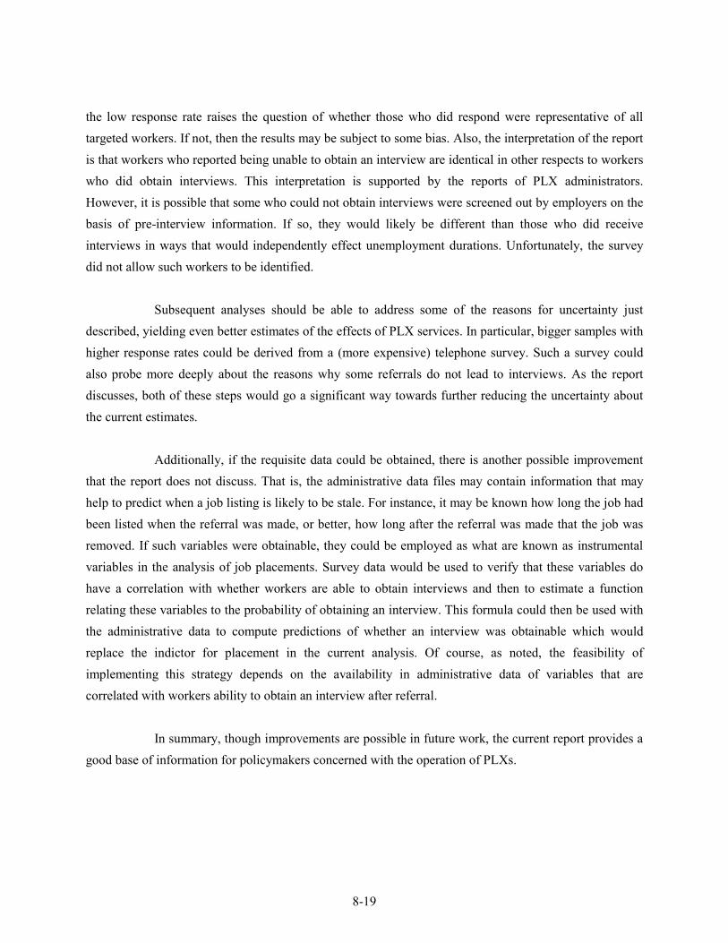
8-19
the low response rate raises the question of whether those who did respond were representative of alltargeted workers. If not, then the results may be subject to some bias. Also, the interpretation of the reportis that workers who reported being unable to obtain an interview are identical in other respects to workerswho did obtain interviews. This interpretation is supported by the reports of PLX administrators.However, it is possible that some who could not obtain interviews were screened out by employers on thebasis of pre-interview information. If so, they would likely be different than those who did receiveinterviews in ways that would independently effect unemployment durations. Unfortunately, the surveydid not allow such workers to be identified.
Subsequent analyses should be able to address some of the reasons for uncertainty justdescribed, yielding even better estimates of the effects of PLX services. In particular, bigger samples withhigher response rates could be derived from a (more expensive) telephone survey. Such a survey couldalso probe more deeply about the reasons why some referrals do not lead to interviews. As the reportdiscusses, both of these steps would go a significant way towards further reducing the uncertainty aboutthe current estimates.
Additionally, if the requisite data could be obtained, there is another possible improvementthat the report does not discuss. That is, the administrative data files may contain information that mayhelp to predict when a job listing is likely to be stale. For instance, it may be known how long the job hadbeen listed when the referral was made, or better, how long after the referral was made that the job wasremoved. If such variables were obtainable, they could be employed as what are known as instrumentalvariables in the analysis of job placements. Survey data would be used to verify that these variables dohave a correlation with whether workers are able to obtain interviews and then to estimate a functionrelating these variables to the probability of obtaining an interview. This formula could then be used withthe administrative data to compute predictions of whether an interview was obtainable which wouldreplace the indictor for placement in the current analysis. Of course, as noted, the feasibility ofimplementing this strategy depends on the availability in administrative data of variables that arecorrelated with workers ability to obtain an interview after referral.
In summary, though improvements are possible in future work, the current report provides agood base of information for policymakers concerned with the operation of PLXs.

8-20
Responses to questions posed in July 24, 2000 letter. Daniel Sullivan 8/31/2000
Q1. Would it be a serious problem if 30 to 50 percent of the referrals and placements wereuntrackable?
A1. It seems clear that being unable to track self-referrals will make it much harder to evaluatethe benefits of PLXs.
Q2. Does it make sense to only track staff-assisted services?
A2. It wouldn’t be logical to base a cost-benefit evaluation of a PLX on all of the costs and onlysome of the benefits and clearly those self-referring obtain some benefits from a PLX.
Q3. Would it be useful to know how benefits are divided between referrals and placements?
A3. Having such an accounting of benefits would be useful.
Q4. Would the use of measures like the entered employment rate create incentives tocream?
A4. The entered-employment rate is not a good measure of the value of a PLX and is likely tolead program administrators to avoid difficult-to-serve populations.
Q5. Should Oregon use the measures of your study?
A5. I think the measures discussed in Chapters 4 and 5 are likely to be superior to the entered-employment rate in judging the value of a PLX and in giving the operators the proper incentives tomaximize the benefits for society.
8.4.4 Comments by Stephen Woodbury
This report describes the results of an extensive study of the impact of the public laborexchange (PLX) on the unemployment duration of jobless workers. The report includes four mainsubstantive chapters. The first (Chapter 3) relies on a mail survey of workers who were referred by theWashington State PLX between January and July 1998. This mail survey, which was sent to 6,000

8-21
referred workers, yielded 587 usable responses. The second (Chapter 4) relies on administrative data onover 300,000 spells of insured unemployment between 1987 and 1995 in Washington State. The third(Chapter 5) uses administrative data on nearly 140,000 spells of insured unemployment during 1995 inOregon. The fourth (Chapter 6) reports on some simulations of the extent to which PLX placementactivities crowd out workers who are not users of the PLX. (Because I am a co-author of Chapter 6, I willhave no comment on that chapter.)
Estimating the impact of the PLX is difficult for two reasons. First, randomized trials areruled out because basic services cannot be denied to workers who desire them. Second, comparisons ofPLX users with nonusers in a nonexperimental evaluation are potentially contaminated by self-selection—workers who use the PLX may different from non-users in ways that may be difficult tocontrol for. Accordingly, the efforts in Chapters 3, 4, and 5 to sort out the impacts of the PLX requiresome innovative and rather clever evaluation designs.
8.4.4.1 Chapter 3
The estimator of PLX impact that is used in Chapter 3 makes use of the survey data andcompares (1) interviewed workers with (2) workers who got a referral and followed up by trying to get aninterview, but then did not get an interview. In terms of Figure 8-1, the comparison is across the third rowfrom the bottom. Interviewed workers may or may not be offered a job, and may or may not accept andreport to the job. Nevertheless, all interviewed workers are compared with workers who tried to get aninterview but did not.
This estimator depends for its appeal on the following logic. Suppose two similar workersare suited to a given job vacancy and are both referred to that vacancy. One follows up immediately, getsthe interview, gets the job offer, and fills the job vacancy. The other waits a day or two and learns that thejob has been filled when he or she calls for an interview. If the logic holds, then this estimator mimicsrandom assignment of workers who come to the ES for referrals—the interviewed workers are analogousto a group of workers randomly assigned to an interview, whereas the workers not interviewed areanalogous to a randomly assigned control group.
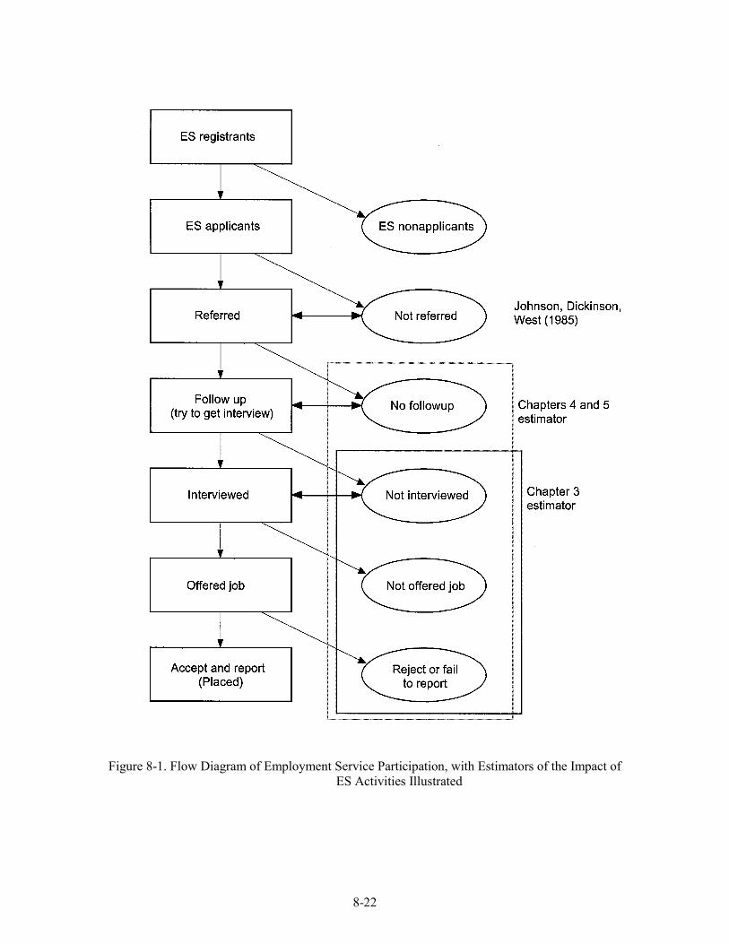
8-22
Figure 8-1. Flow Diagram of Employment Service Participation, with Estimators of the Impact ofES Activities Illustrated

8-23
Accordingly, this is an appealing and original estimator. The authors discuss a possibleweakness associated with this estimator. If a worker does not get an interview because she is, in effect,screened-out by the employer when she calls for an interview, then the comparison between interviewedand not interviewed workers is no longer clean because the two workers were (apparently) not similarafter all. Rather, the worker who didn’t get the interview was rejected based on information obtained overthe telephone. Jacobson argues correctly that this possibility could be tested by a followup interview inwhich workers would be asked why they did not obtain an interview. This is a potentially importantapproach that should be followed up.
8.4.4.2 Chapters 4 and 5
The estimator used in Chapters 4 and 5 can be thought of in either of two ways. First, it canbe thought of as a comparison between placed workers (that is, the bottom left box in Figure 8-1) with thesum of workers who were referred but ultimately were not placed (that is, the sum of workers in thebottom four ovals, which are enclosed by the dashed rectangle labeled “Chapters 4 and 5 estimator”). Thislatter group is the sum of referred workers who (1) did not follow up on a referral, (2) followed up but didnot get an interview, (3) got an interview but were not offered a job, and (4) were offered a job butrejected the offer or did not report.
Alternatively, the estimator used in Chapters 4 and 5 can be thought of as a comparisonbetween workers who followed up on a referral and workers who did not follow up, adjusted for“participation.” Referring to Figure 1, the comparison would be across the fourth row from the bottom,labeled “Chapters 4 and 5 estimator.”
8.4.4.3 Results
The estimates of the impact of the PLX presented in Chapter 3 suggest that PLX placementshave a differential impact on the unemployment spell duration of workers with strong and weak workrecords. For workers with strong records, spell durations are reduced on the order of 7 weeks, whereas forworkers with weak work records, the reduction is somewhat over 3 weeks. Although higher than might beexpected a priori, these are the most convincing existing estimates of the impact of the PLX, in my view.

8-24
8.4.4.4 Importance of Followup Work
For at least three reasons, this study makes clear the importance of further work on theimpact of the PLX. First, the survey approach piloted in this study (and reported in Chapter 3) isextremely promising and deserves to be expanded to other states, in sample size, and in the intensity offollowup. Second, it would be highly useful to supplement the survey of applicants with a survey ofemployers that would obtain data on the circumstances under which an applicant had not obtained a joboffer. Third, given the growing importance of self-referrals, the effectiveness of self-referrals needs to bemonitored and evaluated. Because it tracks self-referrals, Oregon appears to be a natural state in which toexamine and evaluate self-referrals.
8.4.4.5 Responses to Specific Questions
A letter of July 24 requested responses to five specific questions, as follows:
Q1. Would it be a serious problem if 30 to 50 percent of referrals and placements could notbe tracked because applicants have direct access to job contact information?
A1. The answer is clearly yes because if this were the case, there would be no way of detectingwhich applicants made use of PLX services.
Q2. Does it make sense to track only staff-assisted services and not track self-serviceassistance?
A2. No, because increasingly under WIA, the services offered to PLX applicants will be not bestaff assisted. To ignore these would be to ignore a growing proportion of the services and assistanceoffered by PLXs.
Q3. Would it be useful to have information about how benefits are divided among (a)placement effects and referral effects, (b) services delivered early in a claimant’sunemployment spell versus late in a spell, and (c) services delivered to claimants andothers with strong work histories versus those with weak histories?
A3. Yes to all. Interpreting the impact of placements versus referrals is intrinsically interestingand can give insight into how information and matching technologies work. Linking the timing of

8-25
services to program outcomes can tell programs operators when it is most effective to deliver services.Linking the characteristics of applicants to program outcomes can tell programs operators whichapplicants are best served.
Q4. Would the use of the WIA entered-employment and similar measures create incentivesto cream; that is, to provide services to those who are most likely to find jobs on theirown?
A4. Yes, clearly, value-added measures would be superior.
Q5. Now that Oregon has the capacity to create the measures presented in chapters 4 and 5,would you recommend that Oregon use those measures instead of the entered-employment rate and similar measures?
A5. Are the measures presented in the report substantially better that WIA performance measureslike the entered employment rate? Yes in both cases.
8.5 Summary of the Comments of All Four Panelists
This section summarizes the comments of the expert panel in each of six areas:
1. Use of a natural experiment to measure placement effects;
2. Use of nonexperimental methods to measure placement and referral effects;
3. Estimation of displacement effects;
4. Overall benefit-cost computations;
5. Use of the information to improve performance measures; and
6. Tone of the report.
As noted earlier, most of the comments discussed in the section are presented in Section 8.4,but some come from written comments not intended for publication, and some from conversations withthe experts.

8-26
For the most part there was broad agreement among the panel members. In a few cases therewas some disagreement, and not all panelists discussed every issue. Thus, Westat asked the panelists toreview this summary to make sure that it accurately reflects their views.
One preliminary point of importance, all the panelists felt that the term “accurate” needs tobe carefully defined. In this report an accurate estimator is one that produces unbiased estimates that havesmall confidence intervals. In other words, if we used the estimator on repeated trials the differencebetween the “true” effect and the “measured” effect would be small and randomly distributed around the“true” effect.
8.5.1 Use of a Natural Experiment to Measure Placement Effects
All the panelists felt that the identification of referrals made to “stale” listings (those wherethe jobs or interview slots were already filled) could provide unbiased estimates of placement effectsbased on a natural experiment. They agreed that this highly innovative approach provided a means to atleast partially deal with an inability to implement experimental designs that, in the past, made it extremelydifficult to obtain acceptable estimates of the value of PLX direct placement services.
They also agreed that the study’s results should be regarded as illustrative of the method,rather than being close to the “true” value of the effects being measured. Direct confirmation was neededto demonstrate that “disappointed referees” (those job seekers who tried, but failed to obtain interviews)could not secure interviews because the listings were stale, rather than they were screened out byemployers. Several reviewers felt that surveying employers would provide the best evidence about theextent to which referrals were stale, but evidence from job seekers also would be useful.
Also of great importance was surveying a large, representative sample of referred clients toobtain results that would reflect the average placement-effect. The panelists agreed that a comparisongroup of disappointed job-seekers referred to stale listing could be used to measure the effect ofplacements to those listings. However, some panelists noted that there would be cases where placementeffects would be difficult to measure because no disappointed job seekers could be identified. They feltthat determining the extent to which results can be generalized hinges on how different are the jobopenings for which there is, and there is not, a comparison group of disappointed job seekers.

8-27
A final problem that required further analysis was how to treat disappointed job seekers whosubsequently were placed at jobs to which they were referred. No specific recommendations on how todeal with the problem were made, but it seems reasonable to assess how various restrictions oncomparison group measurement affect the results.
8.5.2 Use of Nonexperimental Methods to Measure Placement and Referral Effects
The panelists gave much less attention to the nonexperimental evidence than the potentialnatural experiment. In part this was because the panelists felt that they should defer commenting on thevalidity of the nonexperimental placement estimates until accurate benchmark estimates from the naturalexperiment were obtained. Importantly, the panelists felt that obtaining benchmark estimates based onnatural experiments from at least four states would be needed to assess if a nonexperimental techniquewould produce accurate estimates across all states.
The panelists also agreed that experimental evidence on the validity of the PLX referralestimates could not be obtained. One panelist felt that the biases in the nonexperimental referral-effectestimates could be relatively small because: (1) there was an usually large amount of informationavailable to hold observable differences constant; (2) use of the duration of unemployment may have heldconstant most of the non-observable differences; and (3) the selection bias that tended to lead tounderestimation during the first 10 weeks was balanced by selection bias that tended to lead tooverestimation in the subsequent 16 weeks.
Two other panelists felt that the best evidence to judge referral effects is comparing theestimates in this report to experimental estimates about various types of job search assistance in situationswere services could be withheld. Using that approach they concluded that the Washington referralestimates were more than twice as great as the experimental estimates for programs they felt providedservices with similar effects.
However, it is possible that the experimental results were smaller because the services weredelivered at the point claimants had been unemployed for short periods. Also, the experimental resultsmay have been smaller because the services were not comparable. The panel may not have appreciatedthe total amount of time job seekers spent using PLX services nor the duration of the assistance provided.The inclusion of a table showing that placements often occur after clients obtained a series of referrals

8-28
over many weeks clearly was insufficient. Thus, it would be useful to develop much more preciseinformation about the nature of the PLX services received by study members as part of future work.
The above discussion suggests that a practical way to further assess the accuracy of referralestimates is to carefully review the existing literature on job search assistance to analyze: (1) differencesin the treatments to determine if use of PLXs is likely to have larger effects than the treatments studied;(2) whether timing of the treatments differs in a way that would affect outcomes, and if possible; (3)determine what were the magnitude and direction of selection and other biases in the experimental resultsrelative to nonexperimental estimates. This last piece of evidence could be used to assess whether theadjustments made using the nonexperimental estimators were similar to those made using experimentalestimators.
Finally, the panelists felt that the report would greatly benefit from better explanation of whyan unorthodox approach was used; that is, why placement effects were estimated relative to obtainingreferrals but not being placed, and why referrals not leading to placement effects were estimated relativeto not obtaining referrals (and usually not obtaining any PLX service). In contrast, the conventionalapproach would be to estimate the effect of receiving PLX placement services versus not receiving thoseservices.
The answer is that the conventional estimator can be decomposed into three components: (1)placement effect, (2) referral effect, and (3) looking effect. The total benefits to job seekers equals thesum of the number of individuals in each category times the average effect of each type. The abovedecomposition allows use of the natural experiment discussed in Chapter 3 as a benchmark for assessingthe accuracy of the placement effect estimates. Experimental evidence about similar treatments can helpdetermine if the referral effect estimates are accurate. However, the data used in the study precludedexamining looking effects—comparing those who tried to get a referral, but were unable to do so, to jobseekers who did not use PLX job listings at all. Fortunately, since this last effect is likely to be smallest ofall, and its omission probably leads to only a small underestimate.
8.5.3 Estimation of Displacement Effects
All the panelists were very pleased to see that an attempt was made to assess “crowding-out”or “displacement” effects—the adverse effects on non-users resulting from those receiving PLX aid more

8-29
effectively competing for jobs. There was general agreement that the results were based on the bestavailable methods. However, using those methods require considerably care because the results can behighly sensitive to the assumptions made.
One panelist felt that a fuller discussion of the limitations of the method should be included.Another felt that more should have been made of the single result showing that the crowding-out effectscould be large in periods where jobs were scarce, and there should have been more discussion of how theresults cited in this report compared to those obtained in other studies.
8.5.4 Overall Benefit-cost Computations
The expert panel had a lot to say about the benefit-cost analysis. First, they all seemedpleased that the report made it clear that looking at the benefits versus the costs was the appropriateframework for accessing the value of any government program. Second, they felt that more should havebeen said about:
What benefits should be included in a comprehensive study versus what benefits areactually included.
What are the benefits and costs from the point of view of society, taxpayers, and directbeneficiaries.
Third, they felt that the benefit-cost analysis was not sufficiently refined for use in makingpolicy decisions because the basic estimates of benefits required executing the additional work discussedin Sections 8.5.1 and 8.5.2. In that case, the report’s authors were surprised that so much attention wasgiven to the conceptual framework for the benefit-cost analysis. However, these comments are highlyrelevant in providing guidance for the ongoing PLX study.
Interestingly, some experts focused on the importance of making clear that some benefitsthat should be included were omitted, while others focused more on how costs might be underestimated.Such differences may largely explain why the experts felt including a well-rounded discussion was soimportant to avoid creating the feeling that the report is biased either in favor or against showing that theprogram is cost effective.

8-30
8.5.5 Use of the Information to Improve Performance Measures
There was broad agreement that value-added measures of the type being developed in thisreport would provide highly useful information for assessing overall benefits and for making programchanges that would increase the effectiveness of PLX services. There was equally broad agreement thatthe type of statistics traditionally reported are unsuitable for both of the above purposes.
The panelists were particularly enthusiastic about the prospect of quickly putting into use atleast one accurate value-added measure based on evidence from the natural experiment. Several panelistsfelt that it should be highly feasible to create those measures on an ongoing bases, and agreed with thepoint made in the study, that ongoing estimation of the short-term gains would be a major improvementover existing measures. However, panelists also felt that it would be highly desirable to at least onceconduct the research needed to determine how positive (or negative) were the long-term effects stemmingfrom the length of time matches last, and long term changes in earnings.
They also felt that it was very important to have a comprehensive set of measures that wasnot limited to staff referrals that are currently tracked reasonably well, but also include self referrals that,currently, are only tracked in Oregon.
In general, the panel had no difficulty advocating use of performance measures once theywere validated with experimental evidence. However, they had some reservations about advising programmanagers be provided with potentially flawed value-added measures instead of descriptive statistics thatcertainly are unsuitable for improving performance.
These reservations may stem from a lack of sufficient information to determine use of whichmeasures will do less harm. It is the view of the report’s authors that the additional analysis recommendedby the expert panel would provide the evidence needed to take a more definitive position.
One final issue that was addressed by the experts is whether the new PLX measures wouldcreate incentives to cream—give staff help to clients likely to have the best outcomes, rather than thosewho can be helped the most—and whether such creaming would reduce effectiveness. The view was thatuse of measures like the entered-employment rate would create incentives to cream. However, evidencefrom JTPA programs suggests that creaming may not reduce program effectiveness because thetreatments may have higher returns for eligibles with the best prospect to find work on their own.

8-31
Importantly, creaming incentives can be reduced by regression adjusting the descriptivestatistics to take into account observable differences that affect the employment prospects of participants.These factors include personal characteristics, work histories, and labor market indicators. Also sideconstraints, such as requiring JTPA participants have multiple impediments to being reemployed, canlimit incentives to cream. However, reducing creaming incentives is not at all the same as providingservice providers with the information needed to improve the cost effectiveness of their programs. Onlyvalue-added measures can provide this information.
8.5.6 Tone of the Report
All the panelist felt that the report tended to be much too upbeat in claiming that the positiveresults obtained from the analysis accurately reflected the actual overall benefits for the groups studied.They similarly agreed that overstating the accuracy and applicability of the results made readers lesslikely to believe that PLXs were highly cost effective.
Since much of their discontent stemmed from statements in the executive summary, theauthors thoroughly revised the summary to make it far clearer that: (1) we developed promisingtechniques that, when fully implemented, had the potentially to provide accurate estimates of placementeffects, and (2) the preliminary results indicated that PLXs in Washington and Oregon were highly cost-effective, but those results should be considered as illustrative until additional analysis is completed.
Other changes were made throughout the report to try to correct the impression that point-estimates were highly accurate, and the benefit-cost analysis did more than provide evidence that becausecosts were low per person, relatively small per-person effects would lead to high benefit-cost ratios.
8.6 Implications for Future Analysis
In the view of the report’s authors the expert panel did an outstanding job in pointing out thestrengths and weaknesses of the report. Thus, the panelists made a major contribution to this project, andwe are extremely grateful for their assistance.

8-32
In particular, they clarified the technical econometric issues that need to be addressed inorder to produce results that experts would agree are accurate. They similarly clarified what basic factualinformation about PLX services is needed to provide experts with the background needed to place theeconometric results into an appropriate context. Finally, they made some excellent suggestions about howto use the evidence about reductions in unemployment in producing benefit-cost estimates.
This report’s authors concur with the expert panel’s views about what issues need to beaddressed and what additional work should be carried out. Specifically, we feel that the panel’s findingssuggest taking the following course of action:
1. Top priority should go to surveying employers listing jobs with PLXs to determine theextent to which referrals are made to stale listings and the disappointed referees aredenied interviews based on information obtained by any type of prescreening.
2. Given that Step 1 confirms that many referrals are made to stale listings, the next stepis to obtain survey evidence from a large, representative, sample of placed individualsand individuals referred to the same listings to which those individuals were referredwho tried to obtain interviews, but were unable to do so because the jobs or interviewslots were already filled.
3. These data should be used to estimate placement effects for sample members andassess the applicability of those results to placements made to job listings for whichthere were no disappointed referees to stale listings.
4. The natural experiment evidence should be used as a benchmark for assessing theaccuracy of nonexperimental estimates of placement effects, and adjustments made inthose techniques to improve the accuracy of the nonexperimental estimators.
5. As part of the survey work designed to identify a suitable comparison group, evidenceshould be gathered on the nature and extent of PLX services received by individualswho were referred but not placed by PLXs. Additional information also should becollected about how difficult it is to get to PLX offices and how much time is spentwaiting to obtain assistance, as well as whether referees can figure out which listingsare likely stale.
6. The above survey information as well as additional administrative data on dateslistings are posted should be used as instrumental variables to see if thenonexperimental estimators can be improved.
7. The nonexperimental techniques should be used to examine the relationship betweenshort-term reductions in unemployment and long-term gains in earnings and stabilityof job matches.

8-33
8. Existing evidence on the effectiveness of various forms of job search assistance basedon random-assignment (experimental) designs should be reviewed to assess:
a. How the attributes of services examined in those studies compares to theattributes of PLX services.
b. How much bias there would be had conventional comparison groups andnonexperimental estimation techniques been used instead of control groups.
9. The above information should be used to assess whether the nonexperimentaltechniques used to estimate referral effects are in keeping with reasonableexpectations, as well as whether the bias removed by those techniques is comparableto the bias removed by experimental techniques.
10. New estimates of the benefits to all job-seekers should be developed based on theabove information. The estimates should include appropriate caveats about theaccuracy of various results used, and include a range of estimates when that isappropriate.
11. New estimates of crowding-out effects should be produced based on the benefitestimates. The crowding-out estimates should be subjected to a wider range ofsensitivity analyses and results compared to those of similar studies.
12. Estimates of the adverse effects of using payroll taxes to finance PLXs should beobtained from the existing literature.
13. Benefit-cost estimates should be developed from the above information which clearlydescribe what benefits are included and what are omitted. Estimates of the omittedbenefits should be cited from existing literature, to the extent such estimates exist.
14. The above analysis should be conducted in at least four states with reasonably diversePLXs to determine the extent to which the analytic methods and results can begeneralized.
It is our view that following this outline will produce solid evidence about the overalleffectiveness of PLX direct placement services that experts agree are accurate, and provide a means toprovide policy-makers and program operators with information they can use to improve programeffectiveness. Some attention also should be given to using random-assignment designs to assess thebenefits of viewing listing as well as obtaining staff assistance by claimants who are required toparticipate in profiling and similar programs. Random-assignment designs also should be considered toassess the value of staff assistance for a broad range of PLX clients who would otherwise leave PLXoffices without obtaining such aid.
R-1
REFERENCES
Abraham, Katherine G. (1983) Structural/Frictional vs. Deficient Demand Unemployment: Some NewEvidence. American Economic Review 73, 708–724.
Barnow, Burt S. (1987). “The Impact of CETA Programs on Earnings: A Review of the Literature,”Journal of Human Resources 22(2): 157-193
Barnow, Burt S. and Robert A. Moffit. (1997). “Designs for Evaluating Devolution,” Focus, University ofWisconsin-Madison, Institute for Research on Poverty, (Spring) 59-63.
Bell, Stephen H. et al. (1995). Program Applicants as a Comparison Group in Evaluating TrainingPrograms, Kalamazoo, MI: W.E. Upjohn Institute,
Bloom, Howard S. et al. (1993). The National JTPA Study: Title IIA Impacts on Earnings andEmployment at 18 Months. Washington DC: U.S. Department of Labor, Employment and TrainingAdministration.
Burtless, Gary and Larry L. Orr. (1986). “Are Classical Experiments Needed for Manpower Policy?”Journal of Human Resources 21(4): 606-639
Clark, Kim B., and Summers, Lawrence H. (1982) Unemployment Insurance and Labor MarketTransitions. In M.N. Baily (Ed.), Workers, Jobs, and Inflation (pp. 279-318). Washington, DC:Brookings Institution.
Davidson, Carl, and Woodbury, Stephen A. (1993) The Displacement Effect of Reemployment BonusPrograms. Journal of Labor Economics 11, 575–605.
Davidson, Carl, and Woodbury, Stephen A. (1996) Unemployment Insurance and Unemployment:Implications of the Reemployment Bonus Experiments. In Advisory Council on UnemploymentCompensation: Background Papers, Volume III (pp. KK1–KK37). Washington, DC: U.S.Government Printing Office, 1996.
Ehrenberg, Ronald G. (1980) The Demographic Structure of Unemployment Rates and Labor MarketTransition Probabilities. In R.G. Ehrenberg (Ed.) Research in Labor Economics 3 (pp. 214-291).Greenwich, CT: JAI Press.
Friedlander, Daniel et al. (1997). “Evaluation Government Training Programs for the EconomicallyDisadvantaged,” Journal of Economic Literature, (December) 1809-1855.
Heckman, James J. (1991). “Randomization and Social Policy Evaluation” In Evaluating Welfare andTraining Programs, Charles Manski and Irwin Garfinkel eds. Cambridge, MA; Harvard UniversityPress
Heckman, James J. and Richard R. Robb. (1985). “Alternative Methods for Evaluating the Impact ofInterventions.” In Longitudinal Analysis of Labor Market Data, J. Heckman and B. Singer, eds.Cambridge, MA: Cambridge University Press

R-2
Heckman, J., Lalonde, R., and Smith, J. (1999). “The Economics and Econometrics of Active LaborMarket Program,” Handbook of Labor Economics, Volume 3, Ashenfelter, A. and D. Card, eds.,Amsterdam: Elsevier Science.
Jacobson, Louis S. (1999) Measuring the Effect of Job Service Referrals and Placements on WashingtonState UI Claimants. Rockville, MD: Westat, Inc.
Jacobson, Louis. (1993). “Measuring the Performance of the Claimant Placement Service (CPP) and theEmployment Service (ES) in Aiding Unemployment Insurance (UI) Claimants,” Report to theWashington State Employment Security Department, June 18.
Jacobson, Louis. (1995a). Testimony on the Effectiveness of the U.S. Employment Service andSuggestions for Increasing its Effectiveness; Subcommittee on Human Resources of the Committeeon Ways and Means, U.S. House of Representatives, May 16.
Jacobson, Louis. (1995b). “The Effectiveness of the U.S. Employment Service.” In Advisory Council onUnemployment Compensation: Background Papers, Vol. II. U.S. Government Printing Office.
Johnson, Terry, et al. (1986). “An Evaluation of the Impact of the United States ES Referrals onApplicant Earnings,” Journal of Human Resources 20, 1 (Winter 1985) 117-87
Katz, Arnold, and Louis Jacobson. (1994). Job Search, Employment, Earnings, and the EmploymentService: Comparisons of the Experience of Unemployment Insurance Beneficiaries in Pennsylvania1979-87. W.E. Upjohn Institute Working Paper (Fall)
LaLonde, Robert J. (1986). “Evaluating the Econometric Evaluations of Training Programs withExperimental Data,” American Economic Review 76, 4; (December) 604-620.
Leigh, Duane E. (1990). Does Training Work for Dislocated Workers? A Survey of Existing Evidence.Kalamazoo MI: W.E. Upjohn Institute.
McNeil, Patricia. (1986). The Employment Security System: Preparing for the 21st Century. Committeeon Education and Labor, U.S. House of Representatives, October
Murphy, Kevin M. and Topel, Robert H. (1987) The Evolution of Unemployment in the United States:1968-1985.In Stanley Fischer (Ed.), NBER Macroeconomics Annual 1987 (pp. 11-58). Cambridge,MA: MIT Press.
Spiegelman, Robert G., O’Leary, Christopher J., and Kline, Kenneth J. (1992) The WashingtonReemployment Bonus Experiment: Final Report. Unemployment Insurance Occasional Paper 92–6. Washington, DC: U.S. Department of Labor, Employment and Training Administration.
U.S. Department of Labor, (1986). A Reexamination of the Employment Service: Analysis of PublicComments in Response to the Federal Register Notice, December

Appendix A


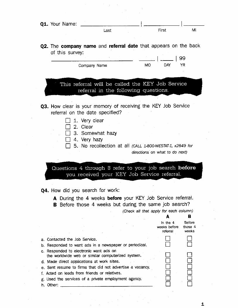


Appendix B

B-1
APPENDIX B
Appendix B-1 is a description of the variables used for the analysis of the Washington StateMail Survey. The variables derived from the mail survey are listed first followed by the variables derivedfrom the UI and ES administrative data. The number of observations, mean, and standard deviation areincluded for each variable.
Appendix B-2 presents the full OLS regression for the Washington State Mail Survey withthe dependent variable being the number of weeks the respondent was unemployed following receipt of areferral. The placement and reasons for not being placed coefficients appear in column 3 of Table 3-6.The regression uses most of the variables listed in Appendix B-1 as independent variables. For eachvariable the parameter estimate, standard error, and the p-value are listed to the right of the variabledescription. The p-value refers to the level of significance for the parameter estimate and p-values lessthan .05 are usually considered statistically significant.

Variable Description N Mean Std DevQ3_1 Recall of Referral: Very Clear 587 0.382 0.486Q3_2 Recall of Referral: Clear 587 0.431 0.496Q3_3 Recall of Referral: Somewhat Hazy 587 0.187 0.391Q4BA Responded to Want Ads: < 4 Weeks Before Referral 587 0.681 0.466Q4BB Responded to Want Ads: 4-8 Weeks Before Referral 587 0.579 0.494Q4CA Responded to E-want Ads: < 4 Weeks Before Referral 587 0.235 0.424Q4CB Responded to E-want Ads: 4-8 Weeks Before Referral 587 0.193 0.395Q4DA Direct Application: < 4 Weeks Before Referral 587 0.627 0.484Q4DB Direct Application: 4-8 Weeks Before Referral 587 0.501 0.500Q4EA Sent Unsolicited Resume: < 4 Weeks Before Referral 587 0.296 0.457Q4EB Sent Unsolicited Resume: 4-8 Weeks Before Referral 587 0.257 0.437Q4FA Acted on Leads from Friends: < 4 Weeks Before Referral 587 0.555 0.497Q4FB Acted on Leads from Friends: 4-8 Weeks Before Referral 587 0.479 0.500Q4GA Private Employment Agency: < 4 Weeks Before Referral 587 0.215 0.411Q4GB Private Employment Agency: 4-8 Weeks Before Referral 587 0.174 0.379Q4HA Other Search Method: < 4 Weeks Before Referral 587 0.065 0.246Q4HB Other Search Method: 4-8 Weeks Before Referral 587 0.083 0.277Q5 Number of Visits to Job Service Before Referral 587 5.874 20.044Q5_MIS Missing: Number of Visits to Job Service Before Referral 587 0.147 0.354Q6A Services Used: Job Search Workshops 587 0.349 0.477Q6B Services Used: Resource Room 587 0.378 0.485Q6C Services Used: Assessment and Counseling 587 0.249 0.433Q6D Services Used: Referral to Training 587 0.162 0.369Q6E Services Used: Referral to Other Assistance 587 0.211 0.409Q7A Number of Jobs Applied for: < 4 Weeks Before Referral 587 5.790 8.684Q7A_MIS Missing: Number of Jobs Applied for: < 4 Weeks Before Referral 587 0.153 0.361Q7B Number of Jobs Applied for: 4-8 Weeks Before Referral 587 5.080 9.922Q7B_MIS Missing: Number of Jobs Applied for: 4-8 Weeks Before Referral 587 0.279 0.449Q8A Number of Interviews Offered Before Referral 587 2.005 2.824Q8A_MIS Missing: Number of Interviews Offered Before Referral 587 0.082 0.274Q8B Number of Interviews Completed Before Referral 587 1.997 2.903Q8B_MIS Missing: Number of Interviews Completed Before Referral 587 0.080 0.272Q8C Number of Job Offers Received Before Referral 587 0.637 0.929Q8C_MIS Missing: Number of Job Offers Received Before Referral 587 0.068 0.252Q8D Number of Job Offers Accepted Before Referral 587 0.484 0.863Q8D_MIS Missing: Number of Job Offers Accepted Before Referral 587 0.126 0.332Q9_NEW Employment Status: Working, Looking for a New Job 587 0.136 0.343Q9_2JB Employment Status: Working, Looking for a Second Job 587 0.032 0.177
Appendix B-1. Description of Variables Used in the WA Mail Survey
Mail Survey Variables
B-2

Variable Description N Mean Std DevQ9_REC Employment Status: Laid-off 587 0.061 0.240Q9_NR6 Employment Status: Not Working Less than Six Months 587 0.494 0.500Q9_GT6 Employment Status: Not Working More than Six Months 587 0.227 0.419Q10 Number of Weeks without Paid Work 587 10.893 28.729Q10_MIS Missing: Number of Weeks without Paid Work 587 0.325 0.469Q11 Number of Weeks Looking for New Employer 587 7.753 11.443Q11_MIS Missing: Number of Weeks Looking for New Employer 587 0.233 0.423Q12_NORS How Referral Received: No Response 587 0.126 0.332Q12_1 How Referral Received: At Job Service Office 587 0.659 0.474Q12_2 How Referral Received: At Library or Public Place 587 0.026 0.158Q12_3 How Referral Received: At Home 587 0.017 0.130Q12_4 How Referral Received: Call from Job Service Office 587 0.119 0.324Q12_5 How Referral Received: Called Job Service 800 Number 587 0.053 0.224Q34A1 Number of Persons in Household 587 2.206 1.745Q34A2 No Other Persons in Household 587 0.145 0.352Q34B1 Number of Persons Earning More than $5,000 587 0.671 0.801Q34B2 No Other Persons Earning More than $5,000 587 0.288 0.457Q35_10K Total Household Income: Less than $10,000 587 0.378 0.485Q35_39K Total Household Income: Between $10,000 and $39,000 587 0.438 0.497Q35_40K Total Household Income: More than $40,000 587 0.138 0.345Q35_MIS Total Household Income: Missing 587 0.000 0.000
AGE Age (Years) 587 36.083 11.205AGE25 Age Less than 25 587 0.201 0.401AGE40 Age Between 25 and 40 587 0.451 0.498AGE54 Age Between 41 and 54 587 0.267 0.443AGE55 Age Greater than 55 587 0.058 0.234AGRI Industry: Agriculture 587 0.051 0.220AREOSP Industry: Aerospace 587 0.015 0.123AVG97 Average Quarterly Earnings in 1997 587 2297.730 2585.330COLLEGE Education: College Degree 587 0.015 0.123EAST East Washington State 587 0.358 0.480ECON_DS1 Program Participant: Economically Disadvantaged 587 0.305 0.461EXP6M Months of Experience Required: 6 587 0.232 0.422EXP12M Months of Experience Required: 12 587 0.220 0.414EXP24M Months of Experience Required: 24 587 0.082 0.274EXP36M Months of Experience Required: 36 587 0.043 0.202EXPMISS Months of Experience Required: Missing 587 0.000 0.000EXPNONE Months of Experience Required: None 587 0.424 0.495FANCY Mail Survey Package: Fancy 587 0.562 0.497
Administrative Variables
B-3

Variable Description N Mean Std DevFEMALE Gender: Female 587 0.475 0.500FOODSTM1 Program Participant: Food Stamp 587 0.014 0.116FULLTIME Hours Required on Job: 40 or More 587 0.670 0.471GRAD Education: Graduate Degree 587 0.138 0.345HDCP_DS1 Program Participant: Handicapped/Disabled 587 0.034 0.182HIGH Education: High School Degree 587 0.394 0.489HIGHWAGE Minimum Acceptable Wage: $13.21 or Higher 587 0.009 0.092HIHR_97 Hours Worked in the Highest Earning Quarter in 1997 587 249.104 231.272HITEN_97 Longest Tenure in the Highest Earning Quarter in 1997 587 1.821 1.373HI_97 Highest Earning Quarter in 1997 587 2985.480 3404.560HRHIWA97 Missing: Hourly Wage of the Highest Earning Quarter in 1997 587 9.262 48.785HSRQ Job Requires High School Degree 587 0.390 0.488IN_SCHO1 Attending School 587 0.048 0.213LESSHIGH Education: Less than High School 587 0.143 0.350LESSHSRQ Job Requires Less than High School Degree 587 0.581 0.494LOWWAGE Minimum Acceptable Wage: $6.59 or Less 587 0.138 0.345LO_97 Lowest Earning Quarter in 1997 587 1318.550 2025.480MAEQUA18 Minimum Age Required: 18 Years 587 0.790 0.407MAGREA18 Minimum Age Required: More than 18 Years 587 0.058 0.234MALESS18 Minimum Age Required: Less than 18 Years 587 0.152 0.359MANU Industry: Manufacturing 587 0.135 0.342MAVG97 Missing: Average 1997 Earnings 587 0.239 0.427MHIHR_97 Missing: Highest Earning Quarter in 1997 587 0.239 0.427MHRHIWA9 Missing: Hourly Wage of Highest Earning Quarter in 1997 587 0.308 0.462MIDWAGE Minimum Acceptable Wage: Between $6.60 and $13.20 587 0.070 0.255MINMISS Minimum Wage Required Not Listed 587 0.775 0.418MINNONE No Minimum Wage Required 587 0.009 0.092MIN_AGE1 Minimum Age Required (Years) 587 15.693 6.286MISS_ED Missing: Education Category 587 0.085 0.279MMINWAGE Missing: Minimum Wage Required 587 0.775 0.418MONEY Mail Survey Package: Extra Money 587 0.080 0.272MOS_EXP1 Months of Experience Required 587 7.876 11.802MOREHSRQ Job Requires More than High School Degree 587 0.029 0.168MRADIVHI Missing: Range in 1997/Highest Earning Quarter in 1997 587 0.239 0.427MSALLES5 Missing: Salary Reported < 50 587 0.065 0.246MSALGRT5 Missing: Salary Reported > 50 587 0.935 0.246MSFW1 Program Participant: Migrant and Seasonal Farm Worker 587 0.015 0.123NOMINAGE No Minimum Age Required 587 0.136 0.343NW Northwest Washington State 587 0.201 0.401OCC_0 Occupational Classification: First Digit 0 587 0.027 0.163OCC_1 Occupational Classification: First Digit 1 587 0.003 0.058
B-4

Variable Description N Mean Std DevOCC_2 Occupational Classification: First Digit 2 587 0.000 0.000OCC_3 Occupational Classification: First Digit 3 587 0.049 0.217OCC_4 Occupational Classification: First Digit 4 587 0.153 0.361OCC_5 Occupational Classification: First Digit 5 587 0.337 0.473OCC_6 Occupational Classification: First Digit 6 587 0.118 0.322OCC_7 Occupational Classification: First Digit 7 587 0.128 0.334OCC_8 Occupational Classification: First Digit 8 587 0.080 0.272OCC_9 Occupational Classification: First Digit 9 587 0.104 0.305OPEN1 Number of Openings for Job Order: 1 587 0.618 0.486OPEN2 Number of Openings for Job Order: 2 587 0.189 0.392OPEN3 Number of Openings for Job Order: 3 587 0.053 0.224OPEN4 Number of Openings for Job Order: 4 587 0.015 0.123OPEN5 Number of Openings for Job Order: 5 587 0.027 0.163OPEN6 Number of Openings for Job Order: 6 587 0.097 0.296OPENING1 Number of Openings for Job Order 587 4.124 14.619OUTC_PLC Placed at the Job Interviewed 587 0.562 0.497OUTC_NSH Accepted Offer, Did not Show Up for Work 587 0.024 0.153OUTC_NAC Did not Accept Offer After Interviewing 587 0.029 0.168OUTC_NOF Did not Obtain Offer After Interviewing 587 0.063 0.243OUTC_NOT Tried, but Failed to Obtain an Interview 587 0.145 0.352OUTC_TRY Did not Try to Obtain Interview 587 0.177 0.382OUTSTATE Outside of Washington State 587 0.009 0.092PARTTIME Hours Required at Job: < 40 587 0.330 0.471PLAIN Mail Survey Package: Plain 587 0.358 0.480QREF_981 Referral Received in Q1 1998 587 0.458 0.499QREF_982 Referral Received in Q2 1998 587 0.542 0.499Q_97_0 Number of Non-zero Quarters in 1997: 0 587 0.239 0.427Q_97_1 Number of Non-zero Quarters in 1997: 1 587 0.095 0.294Q_97_2 Number of Non-zero Quarters in 1997: 2 587 0.138 0.345Q_97_3 Number of Non-zero Quarters in 1997: 3 587 0.174 0.379Q_97_4 Number of Non-zero Quarters in 1997: 4 587 0.354 0.479RADIVHI Range in 1997 Divided by Highest Earning Quarter in 1997 587 0.406 0.363RANGE97 Highest Earning Quarter in 1997 - Lowest Earning Quarter 587 1666.930 2363.150REF1PLC1 Job Order Has One Referral and One Placement 587 0.107 0.310REF1PLC2 Job Order Has One Referral and Two Placements 587 0.034 0.182REF1PLC3 Job Order Has One Referral and Three Placements 587 0.003 0.058REF2PLC1 Job Order Has Two Referrals and One Placement 587 0.099 0.299REF2PLC2 Job Order Has Two Referrals and Two Placements 587 0.036 0.186REF2PLC3 Job Order Has Two Referrals and Three Placements 587 0.000 0.000REF3PLC1 Job Order Has Three Referrals and One Placement 587 0.465 0.499REF3PLC2 Job Order Has Three Referrals and Two Placements 587 0.164 0.370
B-5

Variable Description N Mean Std DevREF3PLC3 Job Order Has Three Referrals and Three Placements 587 0.092 0.289RELOCAT1 Willing to Relocate 587 0.240 0.428RESP Response to Mail Survey 587 1.000 0.000RESP0 Response Type: Unidentified 587 0.271 0.445RESP1 Response Type: Completed Survey 587 0.635 0.482RESP2 Response Type: Returned Without Forwarding Information 587 0.005 0.071RESP3 Response Type: Unidentified 587 0.089 0.284SALARY1 Salary Reported 587 796.078 4564.220SALGRT50 Salary Reported < 50 (Hourly Wage) 587 789.489 4565.360SALLES50 Salary Reported > 50 (Weekly, Monthly, or Annual Wage) 587 6.589 3.417SEATTLE Job-seeker Located in Seattle, Washington 587 0.187 0.391SIC_0 SIC Code: First Digit 0 587 0.051 0.220SIC_1 SIC Code: First Digit 1 587 0.089 0.284SIC_2 SIC Code: First Digit 2 587 0.066 0.249SIC_3 SIC Code: First Digit 3 587 0.068 0.252SIC_4 SIC Code: First Digit 4 587 0.066 0.249SIC_5 SIC Code: First Digit 5 587 0.194 0.396SIC_6 SIC Code: First Digit 6 587 0.039 0.194SIC_7 SIC Code: First Digit 7 587 0.232 0.422SIC_8 SIC Code: First Digit 8 587 0.162 0.369SIC_9 SIC Code: First Digit 9 587 0.032 0.177SOMECOLL Education: Some College 587 0.225 0.418SW Southwest Washington State 587 0.245 0.431TIMBER Industry: Timber 587 0.005 0.071UI_CLAI1 Program Participant: UI Claimant 587 0.417 0.494WHITE Race: White 587 0.835 0.372
B-6

Parameter StandardVariable Estimate Error Prob > |T|
R-Squared 0.415
Intercept 25.451 51.315 0.6202Recall of Referral: Very Clear -0.094 1.038 0.9282Recall of Referral: Clear -0.323 0.955 0.7356Recall of Referral: Somewhat Hazy (Omitted) -- -- --Responded to Want Ads: < 4 Weeks Before Referral 0.540 0.851 0.5263Responded to Want Ads: 4-8 Weeks Before Referral -0.947 0.894 0.2902Responded to E-want Ads: < 4 Weeks Before Referral -0.200 0.907 0.8253Responded to E-want Ads: 4-8 Weeks Before Referral 1.371 1.007 0.1739Direct Application: < 4 Weeks Before Referral -0.331 0.829 0.6903Direct Application: 4-8 Weeks Before Referral -0.286 0.903 0.7520Sent Unsolicited Resume: < 4 Weeks Before Referral -0.678 0.922 0.4627Sent Unsolicited Resume: 4-8 Weeks Before Referral -0.608 1.014 0.5491Acted on Leads from Friends: < 4 Weeks Before Referral -0.267 0.817 0.7435Acted on Leads from Friends: 4-8 Weeks Before Referral -0.481 0.922 0.6020Private Employment Agency: < 4 Weeks Before Referral -0.754 0.929 0.4175Private Employment Agency: 4-8 Weeks Before Referral 0.867 1.009 0.3902Other Search Method: < 4 Weeks Before Referral -2.244 1.643 0.1727Other Search Method: 4-8 Weeks Before Referral 3.433 1.463 ** 0.0194Number of Visits to Job Service Before Referral 0.005 0.018 0.7765Missing: Number of Visits to Job Service Before Referral 2.296 1.086 ** 0.0350Services Used: Job Search Workshops 0.020 0.792 0.9798Services Used: Resource Room -0.648 0.781 0.4073Services Used: Assessment and Counseling -0.649 0.824 0.4315Services Used: Referral to Training 0.203 1.040 0.8457Services Used: Referral to Other Assistance 0.538 0.949 0.5713Number of Jobs Applied for: < 4 Weeks Before Referral 0.116 0.060 * 0.0520Missing: Number of Jobs Applied for: < 4 Weeks Before Referral 1.921 1.250 0.1250Number of Jobs Applied for: 4-8 Weeks Before Referral -0.097 0.052 0.0619Missing: Number of Jobs Applied for: 4-8 Weeks Before Referral -1.640 0.965 * 0.0899Number of Interviews Offered Before Referral -0.396 0.293 0.1760Missing: Number of Interviews Offered Before Referral -1.620 2.499 0.5170Number of Interviews Completed Before Referral 0.568 0.291 * 0.0517Missing: Number of Interviews Completed Before Referral 1.199 2.937 0.6832Number of Job Offers Received Before Referral -0.245 0.541 0.6500Missing: Number of Job Offers Received Before Referral -2.320 2.267 0.3067
Appendix B-2. Regression on Weeks of Unemployment for WA Mail Survey
B-7

Parameter StandardVariable Estimate Error Prob > |T|
Number of Job Offers Accepted Before Referral -0.021 0.554 0.9701Missing: Number of Job Offers Accepted Before Referral 3.186 1.373 ** 0.0208Employment Status: Working, Looking for a New Job 1.430 1.966 0.4676Employment Status: Working, Looking for a Second Job 1.943 2.551 0.4467Employment Status: Laid-off 3.099 2.110 0.1425Employment Status: Not Working Less than Six Months 2.281 1.655 0.1689Employment Status: Not Working More than Six Months 4.694 1.753 *** 0.0077Number of Weeks without Paid Work -0.013 0.014 0.3488Missing: Number of Weeks without Paid Work 0.586 1.000 0.5583Number of Weeks Looking for New Employer 0.038 0.036 0.2876Missing: Number of Weeks Looking for New Employer -2.803 0.976 *** 0.0043How Referral Received: No Response -2.408 1.788 0.1789How Referral Received: At Job Service Office -2.513 1.547 0.1050How Referral Received: At Library or Public Place 0.239 2.610 0.9272How Referral Received: At Home -5.308 3.374 0.1164How Referral Received: Call from Job Service Office -4.512 1.789 ** 0.0120How Referral Received: Called Job Service 800 Number (Omitted) -- -- --Number of Persons in Household 0.309 0.240 0.1986No Other Persons in Household 0.555 1.264 0.6608Number of Persons Earning More than $5,000 -0.286 0.591 0.6281No Other Persons Earning More than $5,000 -1.024 0.965 0.2895Total Household Income: Less than $10,000 0.670 1.680 0.6902Total Household Income: Between $10,000 and $39,000 -0.626 1.659 0.7060Total Household Income: More than $40,000 -0.943 1.923 0.6239Total Household Income: Missing (Omitted) -- -- --Age (Years) 0.068 0.090 0.4535Age Less than 25 -2.696 2.830 0.3414Age Between 25 and 40 -4.128 2.377 * 0.0832Age Between 41 and 54 -2.408 2.407 0.3176Age Greater than 55 -2.456 3.157 0.4371Industry: Agriculture -1.254 2.745 0.6480Industry: Aerospace 0.609 3.225 0.8502Average Quarterly Earnings in 1997 -0.002 0.001 ** 0.0250Education: College Degree -4.713 2.978 0.1143East Washington State 0.358 0.927 0.6998Program Participant: Economically Disadvantaged 1.642 0.935 * 0.0796Months of Experience Required: 6 -0.370 1.861 0.8425Months of Experience Required: 12 0.313 3.519 0.9291Months of Experience Required: 24 -1.118 6.938 0.8720
B-8

Parameter StandardVariable Estimate Error Prob > |T|
Months of Experience Required: 36 -0.713 1.135 0.5304Months of Experience Required: Missing (Omitted) -- -- --Mail Survey Package: Fancy -0.806 0.727 0.2684Gender: Female -0.687 0.882 0.4363Program Participant: Food Stamp 9.004 3.126 *** 0.0042Hours Required on Job: 40 or More 0.619 0.826 0.4539Education: Graduate Degree -2.053 1.223 * 0.0940Program Participant: Handicapped/Disabled 0.331 1.946 0.8651Education: High School Degree 0.080 0.908 0.9295Minimum Acceptable Wage: $13.20 or Higher -13.610 11.110 0.2212Hours Worked in the Highest Earning Quarter in 1997 0.000 0.003 0.9847Longest Tenure in the Highest Earning Quarter in 1997 -0.250 0.628 0.6909Highest Earning Quarter in 1997 0.000 0.000 0.3980Missing: Hourly Wage of the Highest Earning Quarter in 1997 0.001 0.007 0.9369Job Requires High School Degree -2.340 2.439 0.3379Attending School -2.557 1.652 0.1225Education: Less than High School 0.903 1.241 0.4670Job Requires Less than High School Degree -3.574 2.511 0.1553Minimum Acceptable Wage: Less Than $6.60 and $13.20 -7.548 4.460 0.0913Lowest Earning Quarter in 1997 0.002 0.001 ** 0.0111Minimum Age Required: 18 Years 0.666 6.974 0.9240Minimum Age Required: More than 18 Years 0.097 16.418 0.9953Minimum Age Required: Less than 18 Years (Omitted) -- -- --Industry: Manufacturing 2.800 2.581 0.2787Minimum Acceptable Wage: Between $6.60 and $13.20 -10.817 5.332 ** 0.0431Minimum Wage Required Not Listed -4.693 3.623 0.1959No Minimum Wage Required (Omitted) -- -- --Minimum Age Required (Years) -0.449 3.179 0.8877Missing: Education Category 0.741 0.458 0.1063Missing: Minimum Wage Required -1.185 1.374 0.3891Mail Survey Package: Extra Money -1.140 1.354 0.4002Months of Experience Required 0.020 0.135 0.8831Job Requires More than High School Degree (Omitted) -- -- --Program Participant: Migrant and Seasonal Farm Worker -1.199 3.245 0.7119No Minimum Age Required -7.529 50.908 0.8825Northwest Washington State 2.291 1.048 ** 0.0293Number of Openings for Job Order: 1 2.462 2.661 0.3554Number of Openings for Job Order: 2 0.399 2.492 0.8729Number of Openings for Job Order: 3 0.562 2.834 0.8428
B-9
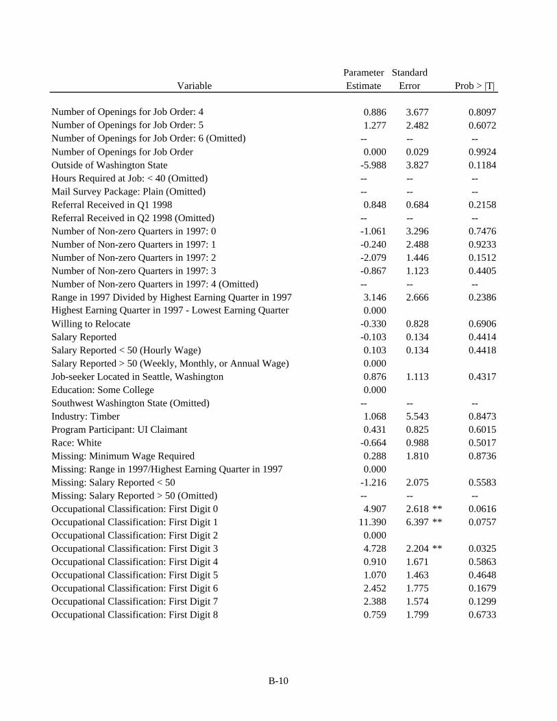
Parameter StandardVariable Estimate Error Prob > |T|
Number of Openings for Job Order: 4 0.886 3.677 0.8097Number of Openings for Job Order: 5 1.277 2.482 0.6072Number of Openings for Job Order: 6 (Omitted) -- -- --Number of Openings for Job Order 0.000 0.029 0.9924Outside of Washington State -5.988 3.827 0.1184Hours Required at Job: < 40 (Omitted) -- -- --Mail Survey Package: Plain (Omitted) -- -- --Referral Received in Q1 1998 0.848 0.684 0.2158Referral Received in Q2 1998 (Omitted) -- -- --Number of Non-zero Quarters in 1997: 0 -1.061 3.296 0.7476Number of Non-zero Quarters in 1997: 1 -0.240 2.488 0.9233Number of Non-zero Quarters in 1997: 2 -2.079 1.446 0.1512Number of Non-zero Quarters in 1997: 3 -0.867 1.123 0.4405Number of Non-zero Quarters in 1997: 4 (Omitted) -- -- --Range in 1997 Divided by Highest Earning Quarter in 1997 3.146 2.666 0.2386Highest Earning Quarter in 1997 - Lowest Earning Quarter 0.000Willing to Relocate -0.330 0.828 0.6906Salary Reported -0.103 0.134 0.4414Salary Reported < 50 (Hourly Wage) 0.103 0.134 0.4418Salary Reported > 50 (Weekly, Monthly, or Annual Wage) 0.000Job-seeker Located in Seattle, Washington 0.876 1.113 0.4317Education: Some College 0.000Southwest Washington State (Omitted) -- -- --Industry: Timber 1.068 5.543 0.8473Program Participant: UI Claimant 0.431 0.825 0.6015Race: White -0.664 0.988 0.5017Missing: Minimum Wage Required 0.288 1.810 0.8736Missing: Range in 1997/Highest Earning Quarter in 1997 0.000Missing: Salary Reported < 50 -1.216 2.075 0.5583Missing: Salary Reported > 50 (Omitted) -- -- --Occupational Classification: First Digit 0 4.907 2.618 ** 0.0616Occupational Classification: First Digit 1 11.390 6.397 ** 0.0757Occupational Classification: First Digit 2 0.000Occupational Classification: First Digit 3 4.728 2.204 ** 0.0325Occupational Classification: First Digit 4 0.910 1.671 0.5863Occupational Classification: First Digit 5 1.070 1.463 0.4648Occupational Classification: First Digit 6 2.452 1.775 0.1679Occupational Classification: First Digit 7 2.388 1.574 0.1299Occupational Classification: First Digit 8 0.759 1.799 0.6733
B-10
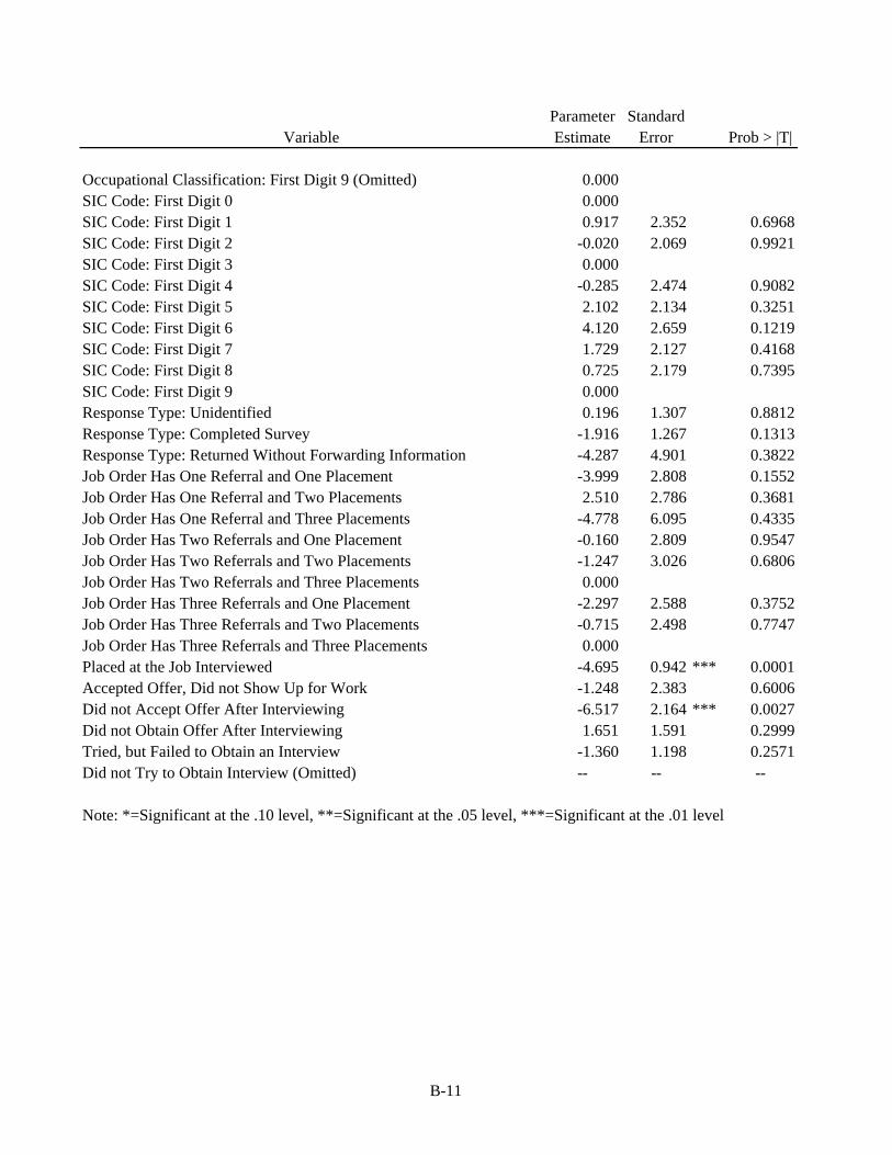
Parameter StandardVariable Estimate Error Prob > |T|
Occupational Classification: First Digit 9 (Omitted) 0.000SIC Code: First Digit 0 0.000SIC Code: First Digit 1 0.917 2.352 0.6968SIC Code: First Digit 2 -0.020 2.069 0.9921SIC Code: First Digit 3 0.000SIC Code: First Digit 4 -0.285 2.474 0.9082SIC Code: First Digit 5 2.102 2.134 0.3251SIC Code: First Digit 6 4.120 2.659 0.1219SIC Code: First Digit 7 1.729 2.127 0.4168SIC Code: First Digit 8 0.725 2.179 0.7395SIC Code: First Digit 9 0.000Response Type: Unidentified 0.196 1.307 0.8812Response Type: Completed Survey -1.916 1.267 0.1313Response Type: Returned Without Forwarding Information -4.287 4.901 0.3822Job Order Has One Referral and One Placement -3.999 2.808 0.1552Job Order Has One Referral and Two Placements 2.510 2.786 0.3681Job Order Has One Referral and Three Placements -4.778 6.095 0.4335Job Order Has Two Referrals and One Placement -0.160 2.809 0.9547Job Order Has Two Referrals and Two Placements -1.247 3.026 0.6806Job Order Has Two Referrals and Three Placements 0.000Job Order Has Three Referrals and One Placement -2.297 2.588 0.3752Job Order Has Three Referrals and Two Placements -0.715 2.498 0.7747Job Order Has Three Referrals and Three Placements 0.000Placed at the Job Interviewed -4.695 0.942 *** 0.0001Accepted Offer, Did not Show Up for Work -1.248 2.383 0.6006Did not Accept Offer After Interviewing -6.517 2.164 *** 0.0027Did not Obtain Offer After Interviewing 1.651 1.591 0.2999Tried, but Failed to Obtain an Interview -1.360 1.198 0.2571Did not Try to Obtain Interview (Omitted) -- -- --
Note: *=Significant at the .10 level, **=Significant at the .05 level, ***=Significant at the .01 level
B-11

Appendix C

C-1
APPENDIX C
Appendix C-1 is a description of the variables used in the Washington State administrativedata analysis. The variables were created from Washington State UI and ES administrative data. Thenumber of observations, mean, and standard deviation are included for each variable.
Appendix C-2 shows the estimates using equation 4.1 with weeks of unemployment as thedependent variable restricted to the referrals and placements made during weeks 10-13. We present theregression for this time period only as an example and the results for the other periods are available uponrequest. For each variable the parameter estimate, standard error, and the p-value are listed to the right ofthe variable description. The p-value refers to the level of significance for the parameter estimate and p-values less than .05 are usually considered statistically significant.
Appendix C-3 shows the estimates using equation 4.1 with UI compensated weeks ofunemployment as the dependent variable restricted to the referrals and placements made during weeks 10-13. We present the regression for this time period only as an example and the results for the other periodsare available upon request. For each variable the parameter estimate, standard error, and the p-value arelisted to the right of the variable description. The p-value refers to the level of significance for theparameter estimate and p-values less than .05 are usually considered statistically significant.

Variable Description N Mean Std DevSP_START Spell Start (SAS Date) 328815 11729.070 842.788WEEK1BEN Weekly Benefit Amount 328815 180.522 74.641PRETENCN Number of Continuous Quarters with Pre-EIN 328815 5.047 5.911JOBCHG Job Change Dummy 328815 2.824 1.838EARN1 Earnings 1 Quarter after Spell Start 324622 2381.750 3179.100EARN2 Earnings 2 Quarters after Spell Start 318199 2946.260 3428.790EARN3 Earnings 3 Quarters after Spell Start 309136 3142.130 3511.340EARN4 Earnings 4 Quarters after Spell Start 297165 3057.980 3489.770EARN5 Earnings 5 Quarters after Spell Start 282423 3025.790 3447.340EARN6 Earnings 6 Quarters after Spell Start 272094 3257.520 3604.110EARN7 Earnings 7 Quarters after Spell Start 259521 3314.310 3661.440EARN8 Earnings 8 Quarters after Spell Start 246365 3186.060 3594.110EARN9 Earnings 9 Quarters after Spell Start 230523 3130.040 3579.950EARN10 Earnings 10 Quarters after Spell Start 218804 3301.290 3704.370EARN11 Earnings 11 Quarters after Spell Start 207699 3336.600 3721.490EARN12 Earnings 12 Quarters after Spell Start 194559 3213.810 3658.550EMP Employment at Month of Spell Start 328815 256372.650 301020.760SP_LNGTH Spell Length Grouped By Ref/Plt Categories 328815 4.316 2.916QTR Quarter of Spell Start 328815 2.587 1.177YEAR Year of Spell Start 328815 1991.600 2.305EDATTAIN Educational Attainment Code 328815 2.987 1.284N0QBASE Number of Non-Zero Quarters in Base Period 328815 3.277 1.193N0QBEFB Number of Non-Zero quarters Year Before 328815 2.798 1.539AGE Age at Start of Spell 328815 35.497 9.904EMP_CHG Employment in Month-Employment in Month 328815 125.406 5136.060UNEMPRTE WA Unemployment Rate in Month of Spell Start 328815 0.076 0.029QTRAFT First Quarter after Spell with Earnings > 0 328815 2.059 1.967IREF1 Indicator of Referral 328815 0.014 0.119IREF2 Indicator of Referral 328815 0.026 0.160IREF3 Indicator of Referral 328815 0.021 0.144IREF4 Indicator of Referral 328815 0.019 0.136IREF5 Indicator of Referral 328815 0.021 0.143IREF6 Indicator of Referral 328815 0.015 0.123IREF7 Indicator of Referral 328815 0.015 0.120IREF8 Indicator of Referral 328815 0.018 0.132IREF9 Indicator of Referral 328815 0.013 0.115IREF10 Indicator of Referral 328815 0.012 0.110IREF11 Indicator of Referral 328815 0.032 0.177IREF12 Indicator of Referral 328815 0.046 0.211
Appendix C.1. Description of Variables Used in the WA Administrative Data
C-2

Variable Description N Mean Std DevIREF13 Indicator of Referral 328815 0.043 0.202IREF14 Indicator of Referral 328815 0.039 0.193IREF15 Indicator of Referral 328815 0.036 0.187IREF16 Indicator of Referral 328815 0.034 0.181IREF17 Indicator of Referral 328815 0.032 0.176IREF18 Indicator of Referral 328815 0.030 0.171IREF19 Indicator of Referral 328815 0.028 0.164IREF20 Indicator of Referral 328815 0.136 0.342IPLT1 Indicator of Placement 328815 0.003 0.051IPLT2 Indicator of Placement 328815 0.009 0.093IPLT3 Indicator of Placement 328815 0.008 0.089IPLT4 Indicator of Placement 328815 0.007 0.084IPLT5 Indicator of Placement 328815 0.008 0.088IPLT6 Indicator of Placement 328815 0.006 0.078IPLT7 Indicator of Placement 328815 0.006 0.078IPLT8 Indicator of Placement 328815 0.008 0.086IPLT9 Indicator of Placement 328815 0.006 0.076IPLT10 Indicator of Placement 328815 0.006 0.075IPLT11 Indicator of Placement 328815 0.014 0.119IPLT12 Indicator of Placement 328815 0.012 0.111IPLT13 Indicator of Placement 328815 0.011 0.106IPLT14 Indicator of Placement 328815 0.011 0.103IPLT15 Indicator of Placement 328815 0.010 0.099IPLT16 Indicator of Placement 328815 0.009 0.094IPLT17 Indicator of Placement 328815 0.009 0.092IPLT18 Indicator of Placement 328815 0.008 0.091IPLT19 Indicator of Placement 328815 0.008 0.088IPLT20 Indicator of Placement 328815 0.047 0.212IAVGBASE Average Base Earnings Inflation Adjusted 328815 4610.280 3707.220ITOTBASE Total Base Earnings Inflation Adjusted 318185 17133.700 13695.460IAVGBEFB Average Earnings Before Base Inflation Adjusted 328815 3995.040 3922.000ITOTBEFB Total Earnings Before Base Inflation Adjusted 299538 15571.890 14605.430WEEKS Number of Weeks in Spell 328815 14.259 13.746QTRAFT4 First Qtr after Spell Earning > 4 x Weekly Benefits 328815 30.626 27.886EMPD Dummy=1 if Emp=. 328815 0.002 0.042EMP_CHGD Dummy=1 if Emp_chg=. 328815 0.002 0.042UNEMPRTD Dummy=1 if Unemprte=. 328815 0.002 0.042SP_TRUNC Dummy=1 if Spell Starts after Q2 1993 328815 0.207 0.405JC234 Job Change Groups 2,3,4 328815 0.161 0.367JC1 Job Change: Retain Job 328815 0.454 0.498JC2 Job Change: No Pre-Spell ID 328815 0.047 0.211
C-3

Variable Description N Mean Std DevJC3 Job Change: Dropout 328815 0.108 0.310JC4 Job Change: Possible Firm ID Change 328815 0.006 0.080JC5 Job Change: Change Job 328815 0.386 0.487Y87 Year 1987 Dummy Variable 328815 0.069 0.253Y88 Year 1988 Dummy Variable 328815 0.061 0.239Y89 Year 1989 Dummy Variable 328815 0.070 0.255Y90 Year 1990 Dummy Variable 328815 0.103 0.305Y91 Year 1991 Dummy Variable 328815 0.143 0.350Y92 Year 1992 Dummy Variable 328815 0.149 0.356Y93 Year 1993 Dummy Variable 328815 0.159 0.365Y94 Year 1994 Dummy Variable 328815 0.156 0.362Y95 Year 1995 Dummy Variable 328815 0.092 0.288QTR_1 Quarter 1 328815 0.258 0.437QTR_2 Quarter 2 328815 0.212 0.408QTR_3 Quarter 3 328815 0.217 0.412QTR_4 Quarter 4 328815 0.314 0.464EDTAIN1 Education: Less than High School 328815 0.095 0.293EDTAIN2 Education: High School 328815 0.106 0.308EDTAIN3 Education: Some College 328815 0.662 0.473EDTAIN4 Education: College 328815 0.108 0.310EDTAIN9 Education: Not Reported 328815 0.029 0.169ABERDEEN WA Job Service Office Location 328815 0.018 0.134AUBURN WA Job Service Office Location 328815 0.048 0.213BELLEVUE WA Job Service Office Location 328815 0.043 0.202BELLINGH WA Job Service Office Location 328815 0.030 0.170BELLTOWN WA Job Service Office Location 328815 0.004 0.061BOEING_E WA Job Service Office Location 328815 0.001 0.032BOEING_R WA Job Service Office Location 328815 0.002 0.039BREMERTO WA Job Service Office Location 328815 0.028 0.165COLUMBIA WA Job Service Office Location 328815 0.009 0.095COLVILLE WA Job Service Office Location 328815 0.013 0.114COWLITZ WA Job Service Office Location 328815 0.031 0.172DATASYS WA Job Service Office Location 328815 0.055 0.228ELLENSBU WA Job Service Office Location 328815 0.006 0.075EVERETT WA Job Service Office Location 328815 0.049 0.216FORKS WA Job Service Office Location 328815 0.004 0.066INVALID WA Job Service Office Location 328815 0.002 0.042LAKEWOOD WA Job Service Office Location 328815 0.052 0.222LEWIS WA Job Service Office Location 328815 0.021 0.143LYNNWOOD WA Job Service Office Location 328815 0.034 0.181MOSES WA Job Service Office Location 328815 0.027 0.163
C-4

Variable Description N Mean Std DevMTVERNON WA Job Service Office Location 328815 0.039 0.194NSEATTLE WA Job Service Office Location 328815 0.031 0.173OKANOGAN WA Job Service Office Location 328815 0.019 0.138OLYMPIA WA Job Service Office Location 328815 0.034 0.181PTANGELE WA Job Service Office Location 328815 0.013 0.114PTTOWNSE WA Job Service Office Location 328815 0.005 0.070PULLMAN WA Job Service Office Location 328815 0.005 0.070RAINIER WA Job Service Office Location 328815 0.036 0.186RAYMOND WA Job Service Office Location 328815 0.006 0.077RENTON WA Job Service Office Location 328815 0.039 0.194RENTGRAD WA Job Service Office Location 328815 0.001 0.029SPOKANE WA Job Service Office Location 328815 0.053 0.223SUNNYSID WA Job Service Office Location 328815 0.036 0.187TACOMA WA Job Service Office Location 328815 0.037 0.189TRICITY WA Job Service Office Location 328815 0.029 0.168VANCOUVE WA Job Service Office Location 328815 0.035 0.185WALLA WA Job Service Office Location 328815 0.013 0.115WENATCHE WA Job Service Office Location 328815 0.035 0.185YAKIMA WA Job Service Office Location 328815 0.057 0.231GEND Gender (0=Male, 1=Female) 328815 0.316 0.465RACE1 Race: White 328815 0.784 0.412RACE2 Race: Black 328815 0.032 0.176RACE3 Race: Hispanic 328815 0.133 0.340RACE4 Race: Native American 328815 0.015 0.122RACE5 Race: Asian 328815 0.022 0.146RACE6 Race: Unknown 328815 0.014 0.118PUB0 Public Assistance: Not Receiving Assistance 328815 0.983 0.128PUB3 Public Assistance: Receiving Assistance 328815 0.004 0.064PUB4 Public Assistance: Family Independence Program 328815 0.002 0.048PUB6 Public Assistance: Status Unknown 328815 0.010 0.101FOOD Registered to Receive Food Stamps 328815 0.014 0.116DISLOCN Dislocated Worker: No 328815 0.819 0.385DISLOC9 Dislocated Worker: Unknown 328815 0.173 0.378DISLOCY Dislocated Worker: Yes 328815 0.008 0.088UISIC0 Industry: Forestry, Agriculture 328815 0.136 0.343UISIC1 Industry: Construction, Mining 328815 0.177 0.382UISIC2 Industry: Non-durable Manufacturing 328815 0.139 0.346UISIC3 Industry: Durable Manufacturing 328815 0.085 0.278UISIC4 Industry: Transportation and Utilities 328815 0.054 0.227UISIC5 Industry: Trade 328815 0.188 0.391UISIC6 Industry: Finance, Insurance, and Real Estate 328815 0.031 0.174
C-5

Variable Description N Mean Std DevUISIC7 Industry: Services 328815 0.083 0.275UISIC8 Industry: Government 328815 0.087 0.283UISIC9 Industry: Other 328815 0.020 0.141I_REF Referred (All Periods) 328815 0.054 0.226I_PLT Placed (All Periods) 328815 0.023 0.150R87 Referred in 1987 328815 0.000 0.019P87 Placed in 1987 328815 0.000 0.020N87 Neither Referred or Placed in 1987 328815 0.068 0.251R88 Referred in 1988 328815 0.001 0.031P88 Placed in 1988 328815 0.001 0.029N88 Neither Referred or Placed in 1988 328815 0.059 0.236R89 Referred in 1989 328815 0.002 0.049P89 Placed in 1989 328815 0.002 0.040N89 Neither Referred or Placed in 1989 328815 0.066 0.248R90 Referred in 1990 328815 0.007 0.084P90 Placed in 1990 328815 0.003 0.057N90 Neither Referred or Placed in 1990 328815 0.093 0.291R91 Referred in 1991 328815 0.009 0.097P91 Placed in 1991 328815 0.004 0.061N91 Neither Referred or Placed in 1991 328815 0.130 0.336R92 Referred in 1992 328815 0.009 0.094P92 Placed in 1992 328815 0.004 0.060N92 Neither Referred or Placed in 1992 328815 0.136 0.343R93 Referred in 1993 328815 0.009 0.093P93 Placed in 1993 328815 0.003 0.059N93 Neither Referred or Placed in 1993 328815 0.146 0.353R94 Referred in 1994 328815 0.010 0.098P94 Placed in 1994 328815 0.004 0.061N94 Neither Referred or Placed in 1994 328815 0.142 0.349R95 Referred in 1995 328815 0.006 0.080P95 Placed in 1995 328815 0.002 0.049N95 Neither Referred or Placed in 1995 328815 0.083 0.275RECREF Referred and Job Change: Retain Job 328815 0.019 0.136RECPLT Placed and Job Change: Retain Job 328815 0.009 0.095RECNEI Neither Referred or Placed and Job Change: Retain Job 328815 0.426 0.494J234REF Referred and Job Change Groups 2,3,4 328815 0.009 0.092J234PLT Placed and Job Change Groups 2,3,4 328815 0.003 0.055J234NEI Neither Referred or Placed and Job Change Groups 2,3,4 328815 0.149 0.356CHAREF Referred and Job Change: Change Job 328815 0.027 0.161CHAPLT Placed and Job Change: Change Job 328815 0.011 0.105CHANEI Neither Referred or Placed and Job Change: Change Job 328815 0.348 0.476
C-6
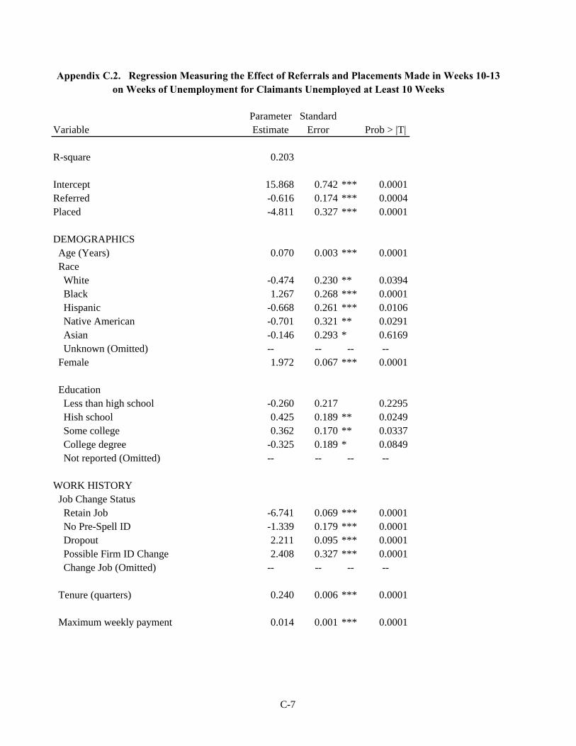
Parameter StandardVariable Estimate Error Prob > |T|
R-square 0.203
Intercept 15.868 0.742 *** 0.0001Referred -0.616 0.174 *** 0.0004Placed -4.811 0.327 *** 0.0001
DEMOGRAPHICS Age (Years) 0.070 0.003 *** 0.0001 Race White -0.474 0.230 ** 0.0394 Black 1.267 0.268 *** 0.0001 Hispanic -0.668 0.261 *** 0.0106 Native American -0.701 0.321 ** 0.0291 Asian -0.146 0.293 * 0.6169 Unknown (Omitted) -- -- -- -- Female 1.972 0.067 *** 0.0001
Education Less than high school -0.260 0.217 0.2295 Hish school 0.425 0.189 ** 0.0249 Some college 0.362 0.170 ** 0.0337 College degree -0.325 0.189 * 0.0849 Not reported (Omitted) -- -- -- --
WORK HISTORY Job Change Status Retain Job -6.741 0.069 *** 0.0001 No Pre-Spell ID -1.339 0.179 *** 0.0001 Dropout 2.211 0.095 *** 0.0001 Possible Firm ID Change 2.408 0.327 *** 0.0001 Change Job (Omitted) -- -- -- --
Tenure (quarters) 0.240 0.006 *** 0.0001
Maximum weekly payment 0.014 0.001 *** 0.0001
Appendix C.2. Regression Measuring the Effect of Referrals and Placements Made in Weeks 10-13on Weeks of Unemployment for Claimants Unemployed at Least 10 Weeks
C-7

Parameter StandardVariable Estimate Error Prob > |T|
Earnings 5-8 quarters before spell 0.000 0.000 *** 0.0001 Earnings 1-4 quarters before spell 0.000 0.000 *** 0.0001
LABOR MARKET Employment 0.000 0.000 0.4486 Employment Change -0.113 0.000 ** 0.0496 Unemployment rate 0.407 2.334 0.8616
YEAR 1987 3.090 0.299 *** 0.0001 1988 3.323 0.279 *** 0.0001 1989 2.726 0.264 *** 0.0001 1990 3.655 0.254 *** 0.0001 1991 8.571 0.243 *** 0.0001 1992 10.361 0.236 *** 0.0001 1993 7.076 0.232 *** 0.0001 1994 3.760 0.148 *** 0.0001 1995 (Omitted) -- -- -- --
QUARTER 1 -0.250 0.091 *** 0.0057 2 1.750 0.085 *** 0.0001 3 1.234 0.085 *** 0.0001 4 (Omitted) -- -- -- --
PROGRAM PARTICIPATION Registered to collect Food Stamps 0.825 0.236 *** 0.0005
Public Assistance Status Not receiving public assistance -0.896 0.267 *** 0.0008 Receiving public assistance -0.298 0.514 0.5625 In Family Independence program -1.258 0.624 ** 0.0439 Status unknown (Omitted) -- -- -- --
Dislocated Worker Status Not a dislocated worker -3.459 0.334 *** 0.0001 Maybe a dislcated worker -1.983 0.326 *** 0.0001 Definitely a dislocated worker (Omitted) -- -- -- --
C-8

Parameter StandardVariable Estimate Error Prob > |T|
INDUSTRY (1-digit SIC) 1. Forestry, Agriculture -1.152 0.212 *** 0.0001 2. Construction, Mining -1.876 0.203 *** 0.0001 3. Non-durable manufacturing -0.456 0.208 ** 0.0286 4. Durable manufacturing 0.468 0.213 ** 0.0281 5. Transportation and Utilities -0.693 0.226 *** 0.0022 6. Trade -0.129 0.199 0.5168 7. Finance, Insurance, and Real Estate -0.221 0.237 0.3512 8. Services 0.032 0.210 0.8795 9. Government -0.144 0.208 0.4888 10. Other (Omitted) -- -- -- --
Spell Truncated -1.768 0.176 *** 0.0001
JOB SERVICE OFFICE ABERDEEN 2.459 0.308 *** 0.0001 AUBURN 2.806 1.775 0.1139 BELLEVUE 1.874 1.776 0.2916 BELLINGH 0.060 0.260 0.8182 BELLTOWN 3.314 1.837 * 0.0713 BOEING_E 11.368 0.924 *** 0.0001 BOEING_R 2.330 1.880 0.2152 BREMERTO 1.349 0.271 *** 0.0001 COLUMBIA -0.153 0.384 0.6908 COLVILLE 0.354 0.349 0.3112 COWLITZ 0.191 0.287 0.5063 DATASYS -0.675 0.239 *** 0.0047 ELLENSBU 0.603 0.437 0.1676 EVERETT 1.011 0.429 ** 0.0185 FORKS -0.302 0.581 0.6032 INVALID -0.081 0.798 0.9194 LAKEWOOD 1.570 0.459 *** 0.0006 LEWIS -0.397 0.315 0.2076 LYNNWOOD 0.370 0.437 0.3975 MOSES -0.462 0.280 * 0.0984 MTVERNON -0.019 0.255 0.9420 NSEATTLE 2.540 1.776 0.1528 OKANOGAN -1.075 0.313 *** 0.0006 OLYMPIA 0.794 0.259 *** 0.0022
C-9

Parameter StandardVariable Estimate Error Prob > |T|
PTANGELE 0.222 0.365 0.5432 PTTOWNSE 0.960 0.477 ** 0.0444 PULLMAN -1.718 0.542 *** 0.0015 RAINIER 3.772 1.774 ** 0.0335 RAYMOND 0.061 0.459 0.8948 RENTON 2.590 1.774 0.1442 RENTGRAD 2.859 2.073 0.1679 SPOKANE 1.008 0.294 *** 0.0006 SUNNYSID -0.149 0.209 0.4765 TACOMA 1.176 0.465 ** 0.0114 TRICITY -0.734 0.246 *** 0.0029 VANCOUVE -0.179 0.278 0.5205 WALLA -1.202 0.349 *** 0.0006 WENATCHE -0.696 0.257 *** 0.0067 YAKIMA (Omitted) -- -- -- --
Note: *=Significant at the .10 level, **=Significant at the .05 level, ***=Significant at the .01 level
C-10

Parameter StandardVariable Estimate Error Prob > |T|
R-square 0.346
Intercept 25.323 1.525 *** 0.0001Referred -2.460 0.358 *** 0.0001Placed 12.388 0.671 *** 0.0001
DEMOGRAPHICS Age (Years) 0.046 0.006 *** 0.0001 Race White -0.746 0.473 0.1150 Black -1.169 0.551 ** 0.0338 Hispanic -4.322 0.537 *** 0.0001 Native American 0.873 0.660 0.1856 Asian -0.012 0.601 0.9835 Unknown (Omitted) -- -- -- -- Female 1.344 0.138 *** 0.0001
Education Less than high school -3.599 0.445 *** 0.0001 Hish school -0.351 0.389 0.3676 Some college -0.874 0.350 ** 0.0124 College degree -0.194 0.388 0.6163 Not reported (Omitted) -- -- -- --
WORK HISTORY Job Change Status Retain Job 10.961 0.141 *** 0.0001 No Pre-Spell ID -1.160 0.368 *** 0.0016 Dropout 40.221 0.196 *** 0.0001 Possible Firm ID Change 44.492 0.672 *** 0.0001 Change Job (Omitted) -- -- -- --
Tenure (quarters) 0.108 0.011 *** 0.0001
Maximum weekly payment 0.025 0.001 *** 0.0001
Appendix C.3. Regression Measuring the Effect of Referrals and Placements Made in Weeks 10-13on UI Compensated Weeks of Unemployment for Claimants Unemployed at Least 10 Weeks
C-11

Parameter StandardVariable Estimate Error Prob > |T|
Earnings 5-8 quarters before spell 0.000 0.000 *** 0.0001 Earnings 1-4 quarters before spell 0.000 0.000 *** 0.0001
LABOR MARKET Employment 0.000 0.000 *** 0.0030 Employment Change 0.000 0.000 *** 0.0008 Unemployment rate -10.230 4.794 ** 0.0329
YEAR 1987 11.648 0.613 *** 0.0001 1988 14.116 0.573 *** 0.0001 1989 13.029 0.542 *** 0.0001 1990 14.094 0.521 *** 0.0001 1991 16.511 0.500 *** 0.0001 1992 15.350 0.484 *** 0.0001 1993 14.076 0.476 *** 0.0001 1994 11.474 0.304 *** 0.0001 1995 (Omitted) -- -- -- --
QUARTER 1 0.549 0.186 *** 0.0031 2 2.775 0.175 *** 0.0001 3 1.414 0.175 *** 0.0001 4 (Omitted) -- -- -- --
PROGRAM PARTICIPATION Registered to collect Food Stamps 4.365 0.484 *** 0.0001
Public Assistance Status Not receiving public assistance -5.562 0.549 *** 0.0001 Receiving public assistance -5.198 1.056 *** 0.0001 In Family Independence program 0.112 1.283 0.9301 Status unknown (Omitted) -- -- -- --
Dislocated Worker Status Not a dislocated worker -0.177 0.686 0.7968 Maybe a dislcated worker -1.188 0.670 * 0.0763 Definitely a dislocated worker (Omitted) -- -- -- --
C-12

Parameter StandardVariable Estimate Error Prob > |T|
INDUSTRY (1-digit SIC) 1. Forestry, Agriculture 1.846 0.435 *** 0.0001 2. Construction, Mining -3.944 0.418 *** 0.0001 3. Non-durable manufacturing -0.768 0.428 * 0.0726 4. Durable manufacturing 0.539 0.438 0.2184 5. Transportation and Utilities -1.898 0.464 *** 0.0001 6. Trade 0.069 0.408 0.8663 7. Finance, Insurance, and Real Estate 0.059 0.486 0.9029 8. Services 0.814 0.431 * 0.0588 9. Government 0.202 0.426 0.6354 10. Other (Omitted) -- -- -- --
Spell Truncated -1.940 0.362 *** 0.0001
JOB SERVICE OFFICE ABERDEEN 2.129 0.633 *** 0.0008 AUBURN 14.474 3.646 *** 0.0001 BELLEVUE 13.681 3.649 *** 0.0002 BELLINGH 1.741 0.534 *** 0.0011 BELLTOWN 10.325 3.774 *** 0.0062 BOEING_E 14.502 1.898 *** 0.0001 BOEING_R 20.968 3.862 *** 0.0001 BREMERTO 5.105 0.557 *** 0.0001 COLUMBIA 7.599 0.789 *** 0.0001 COLVILLE 4.203 0.717 *** 0.0001 COWLITZ 3.195 0.590 *** 0.0001 DATASYS 7.460 0.490 *** 0.0001 ELLENSBU 0.925 0.897 0.3025 EVERETT 5.678 0.881 *** 0.0001 FORKS 2.492 1.194 ** 0.0370 INVALID 1.586 1.639 0.3333 LAKEWOOD 6.425 0.943 *** 0.0001 LEWIS 0.629 0.648 0.3317 LYNNWOOD 4.958 0.898 *** 0.0001 MOSES -0.879 0.574 0.1259 MTVERNON 1.427 0.524 *** 0.0064 NSEATTLE 13.462 3.649 0.0002 OKANOGAN -0.482 0.643 0.4539 OLYMPIA 2.471 0.532 *** 0.0001
C-13

Parameter StandardVariable Estimate Error Prob > |T|
PTANGELE -0.345 0.750 0.6453 PTTOWNSE 4.470 0.981 *** 0.0001 PULLMAN 4.508 1.113 *** 0.0001 RAINIER 15.508 3.644 *** 0.0001 RAYMOND -1.061 0.942 0.2599 RENTON 13.190 3.644 *** 0.0003 RENTGRAD 8.818 4.258 ** 0.0384 SPOKANE 3.799 0.605 *** 0.0001 SUNNYSID -1.076 0.429 ** 0.0122 TACOMA 6.087 0.955 *** 0.0001 TRICITY 0.402 0.505 0.4263 VANCOUVE 8.472 0.571 *** 0.0001 WALLA 2.163 0.717 *** 0.0026 WENATCHE -3.380 0.527 *** 0.0001 YAKIMA (Omitted) -- -- -- --
Note: *=Significant at the .10 level, **=Significant at the .05 level, ***=Significant at the .01 level
C-14

Appendix D

D-1
APPENDIX D
Appendix D-1 is a list of the variables used in the Oregon State administrative data analysis.The variables were created from Oregon State UI and ES administrative data by staff from the OregonEmployment Department (OED). The number of observations, mean, and standard deviation are includedfor each variable.
Appendix D-2 shows the estimates using equation 4.1 with weeks of unemployment as thedependent variable restricted to the referrals and placements made during weeks 10-13. We present theregression for this time period only as an example and the results for the other periods are available uponrequest. For each variable the parameter estimate, standard error, and the p-value are listed to the right ofthe variable description. The p-value refers to the level of significance for the parameter estimate and p-values less than .05 are usually considered statistically significant.
Appendix D-3 shows the estimates using equation 4.1 with UI compensated weeks ofunemployment as the dependent variable restricted to the referrals and placements made during weeks 10-13. We present the regression for this time period only as an example and the results for the other periodsare available upon request. For each variable the parameter estimate, standard error, and the p-value arelisted to the right of the variable description. The p-value refers to the level of significance for theparameter estimate and p-values less than .05 are usually considered statistically significant.

Variable N Mean Std Dev
SPLNGTH 58980 20.190 7.150 Spell lengthBSYRWGE 58980 16944.123 12404.629 Base-year wageRWBA 58980 186.810 83.080 Weekly benefit amountSEX 58980 0.580 0.490 Male = 1, Female = 0BSYRWEEK 58980 40.800 10.980CLAIMAGE 58980 37.460 10.230 Age in yearsWRACE 58980 0.850 0.350 1 = white, 0 = otherHRACE 58980 0.077 0.270 1 = Hispanic, 0 = otherARACE 58980 0.018 0.130 1 = American Indian, 0 = otherIRACE 58980 0.021 0.140 1 = other than African AmericanSICA 58980 0.045 0.210 Industry DummiesSICB 58980 0.002 0.044SICC 58980 0.095 0.290SICD 58980 0.230 0.420SICE 58980 0.047 0.210SICF 58980 0.061 0.240SICG 58980 0.180 0.390SICH 58980 0.044 0.200SICI 58980 0.240 0.430SICJ 58980 0.042 0.200BAKE 58980 0.009 0.095 Office DummiesCROO 58980 0.007 0.083DOUGLA 58980 0.037 0.190HARNE 58980 0.004 0.067JEFFERS 58980 0.006 0.074JOSEPHI 58980 0.028 0.160KLAMAT 58980 0.024 0.150SHERMA 58980 0.001 0.025UMATILL 58980 0.025 0.160UNIO 58980 0.010 0.098WASC 58980 0.010 0.099WASHING 58980 0.086 28.000SameEmp 58980 0.220 0.410 Recalled = 1EMPCHG 58980 9.860 15.620 Local area employment change (2)QTR1SPST 58980 0.200 0.400 Spell start quarter 1 = 1, other = 0QTR2SPST 58980 0.220 0.420 Spell start quarter 2 = 2, other = 0QTR3SPST 58980 0.200 0.400 Spell start quarter 3 = 3, other = 0QTR4SPST 58980 0.380 0.490 Spell start quarter 4 = 4, other = 0
Appendix D.1. Description of Variables Used in the OR Administrative Data
D-2

Variable N Mean Std DevYR95SPST 58980 1.000 0.000 Spell start in 1995DOT_01 58980 0.210 0.400 Occupation DummiesDOT_2 58980 0.210 0.410DOT_3 58980 0.120 0.330DOT_4 58980 0.071 0.260DOT_5 58980 0.043 0.200DOT_6 58980 0.068 0.250DOT_7 58980 0.036 0.190DOT_8 58980 0.100 0.300ESREF4 58980 0.041 0.200 Referred in weeks 10-13ESPLT4 58980 0.003 0.056 Placed in weeks 10-13UNEMPSP 58980 80.360 7.340 Unemployment rate x 10 in local areaEMPSP 58980 1656.200 24.670 Employment in local areaDENSITY 58980 329.280 489.810 Local area density (pop./sq. mile)AGESQ 58980 1507.980 796.930 Age squaredREPWAGE 58980 0.312 0.070 Replacement wage (WBA/high qtr. earning)
D-3

Parameter StandardVariable Estimate Error Prob > |T|
R-squared 0.095
(Constant) 59.993 11.510 *** 0.0000BSYRWGE 0.000 0.000 *** 0.0000 Base-year wageRWBA -0.004 0.001 *** 0.0030 Weekly benefit amountSEX -0.230 0.147 0.1170 Male = 1, Female = 0BSYRWEEK -0.133 0.007 *** 0.0000CLAIMAGE 0.081 0.043 * 0.0580 Age in yearsWRACE 0.465 0.355 0.1900 1 = white, 0 = otherHRACE -0.046 0.427 0.9140 1 = Hispanic, 0 = otherARACE 1.132 0.564 ** 0.0450 1 = American Indian, 0 = otherIRACE 0.964 0.549 * 0.0790 1 = other than African AmericanSICA -2.498 0.608 *** 0.0000 Industry DummiesSICB -5.931 1.463 *** 0.0000SICC -2.778 0.557 *** 0.0000SICD -1.714 0.529 *** 0.0010SICE -2.934 0.587 *** 0.0000SICF -2.877 0.569 *** 0.0000SICG -2.649 0.536 *** 0.0000SICH -3.752 0.593 *** 0.0000SICI -3.055 0.532 *** 0.0000SICJ -1.514 0.596 ** 0.0110BAKE 1.765 0.637 *** 0.0060 Office DummiesCROO 3.262 0.729 *** 0.0000DOUGLA 1.196 0.324 *** 0.0000HARNE -1.733 0.910 * 0.0570JEFFERS 2.067 0.816 ** 0.0110JOSEPHI 2.275 0.370 *** 0.0000KLAMAT 0.600 0.398 0.1310SHERMA 5.828 2.369 ** 0.0140UMATILL 1.408 0.394 *** 0.0000UNIO 0.280 0.620 0.6520WASC -0.761 0.611 0.2130WASHING -0.870 0.220 *** 0.0000SameEmp -10.052 0.155 *** 0.0000 Recalled = 1EMPCHG 0.032 0.009 *** 0.0000 Local area employment change (2)
Appendix D.2. Regression Measuring the Effect of Referrals and Placements Made in Weeks 10-13on Weeks of Unemployment for Claimants Unemployed at Least 10 Weeks
D-4

Parameter StandardVariable Estimate Error Prob > |T|
QTR1SPST 5.993 0.687 *** 0.0000 Spell start quarter 1 = 1, other = 0QTR2SPST 0.840 0.236 *** 0.0000 Spell start quarter 2 = 2, other = 0QTR3SPST 2.075 0.258 *** 0.0000 Spell start quarter 3 = 3, other = 0DOT_01 0.583 0.231 ** 0.0120 Occupation DummiesDOT_2 0.309 0.228 0.1760DOT_3 -0.252 0.256 0.3250DOT_4 -0.105 0.307 0.7310DOT_5 1.345 0.348 *** 0.0000DOT_6 1.542 0.287 *** 0.0000DOT_7 0.861 0.364 ** 0.0180DOT_8 0.635 0.264 ** 0.0160ESREF4 -2.781 0.306 *** 0.0000 Referred in weeks 10-13ESPLT4 -6.943 1.085 *** 0.0000 Placed in weeks 10-13UNEMPSP -0.205 0.021 *** 0.0000 Unemployment rate x 10 in local areaEMPSP -0.006 0.007 0.4200 Employment in local areaDENSITY 0.000 0.000 0.9250 Local area density (pop./sq. mile)AGESQ -0.001 0.001 0.3490 Age squaredREPWAGE -4.859 1.078 *** 0.0000 Replacement wage (WBA/high qtr. earning)
Note: *=Significant at the .10 level, **=Significant at the .05 level, ***=Significant at the .01 level
D-5

Parameter StandardVariable Estimate Error Prob > |T|
R-squared 0.105
(Constant) 75.055 5.341 *** 0.0000BSYRWGE 0.000 0.000 *** 0.0000 Base-year wageRWBA 0.009 0.001 *** 0.0000 Weekly benefit amountSEX -0.558 0.068 *** 0.0000 Male = 1, Female = 0BSYRWEEK 0.059 0.003 *** 0.0000CLAIMAGE 0.208 0.020 *** 0.0000 Age in yearsWRACE -0.425 0.165 ** 0.0120 1 = white, 0 = otherHRACE -0.433 0.198 ** 0.0290 1 = Hispanic, 0 = otherARACE 0.027 0.262 0.9170 1 = American Indian, 0 = otherIRACE -0.035 0.255 0.8910 1 = other than African AmericanSICA -0.179 0.282 0.5270 Industry DummiesSICB -1.280 0.679 * 0.0590SICC -0.654 0.259 ** 0.0110SICD 0.745 0.246 *** 0.0020SICE -0.048 0.272 0.8600SICF 0.311 0.264 0.2390SICG 0.057 0.249 0.8180SICH 0.452 0.275 0.1010SICI 0.074 0.247 0.7640SICJ 0.004 0.277 0.9890BAKE -1.162 0.295 *** 0.0000 Office DummiesCROO 0.381 0.338 0.2600DOUGLA 0.547 0.150 *** 0.0000HARNE -1.438 0.422 *** 0.0010JEFFERS -0.354 0.379 0.3500JOSEPHI 0.766 0.172 *** 0.0000KLAMAT 0.422 0.285 ** 0.0220SHERMA 1.525 1.099 0.1660UMATILL -0.623 0.183 *** 0.0010UNIO -1.185 0.287 *** 0.0000WASC -0.097 0.284 0.7320WASHING -0.322 0.102 *** 0.0020SameEmp -3.252 0.072 *** 0.0000 Recalled = 1EMPCHG -0.014 0.004 *** 0.0010 Local area employment change (2)
Appendix D.3. Regression Measuring the Effect of Referrals and Placements Made in Weeks 10-13on UI Compensated Weeks of Unemployment for Claimants Unemployed at Least 10 Weeks
D-6
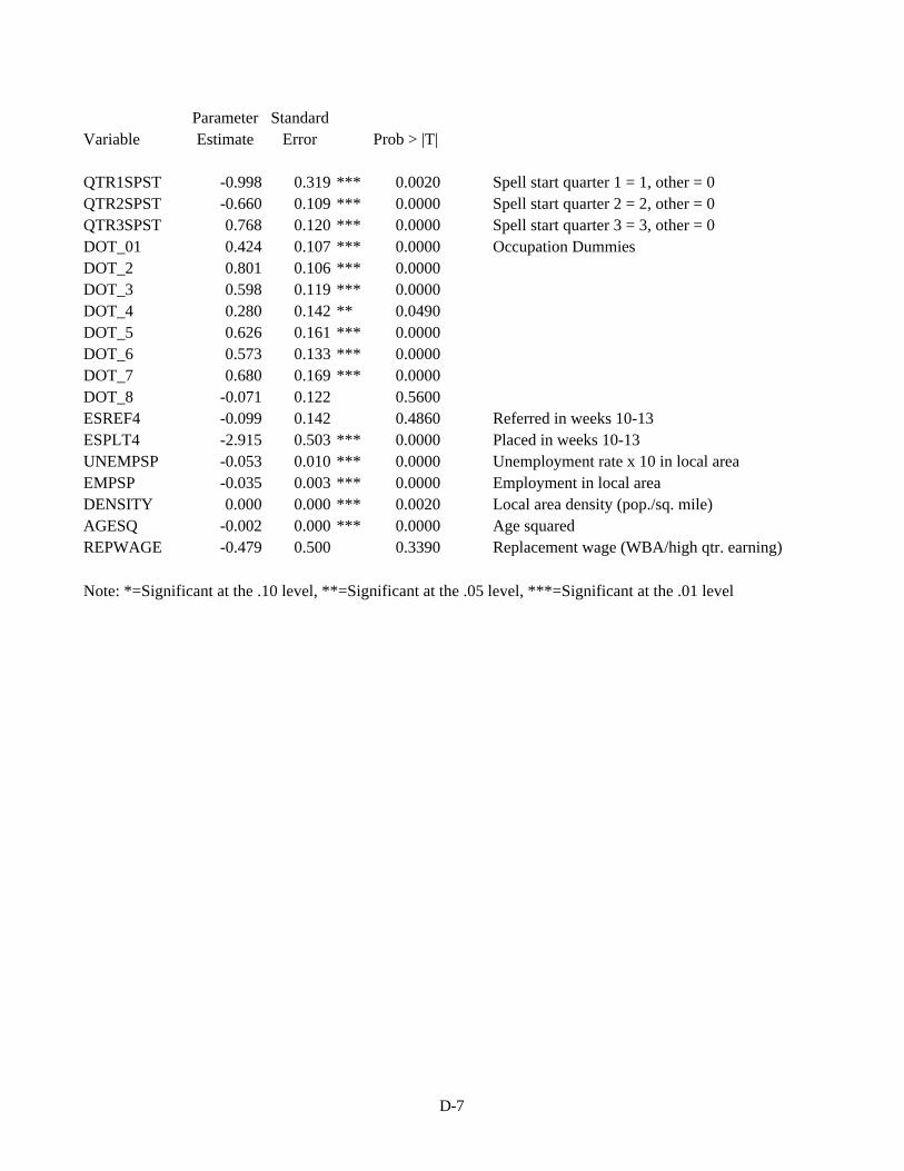
Parameter StandardVariable Estimate Error Prob > |T|
QTR1SPST -0.998 0.319 *** 0.0020 Spell start quarter 1 = 1, other = 0QTR2SPST -0.660 0.109 *** 0.0000 Spell start quarter 2 = 2, other = 0QTR3SPST 0.768 0.120 *** 0.0000 Spell start quarter 3 = 3, other = 0DOT_01 0.424 0.107 *** 0.0000 Occupation DummiesDOT_2 0.801 0.106 *** 0.0000DOT_3 0.598 0.119 *** 0.0000DOT_4 0.280 0.142 ** 0.0490DOT_5 0.626 0.161 *** 0.0000DOT_6 0.573 0.133 *** 0.0000DOT_7 0.680 0.169 *** 0.0000DOT_8 -0.071 0.122 0.5600ESREF4 -0.099 0.142 0.4860 Referred in weeks 10-13ESPLT4 -2.915 0.503 *** 0.0000 Placed in weeks 10-13UNEMPSP -0.053 0.010 *** 0.0000 Unemployment rate x 10 in local areaEMPSP -0.035 0.003 *** 0.0000 Employment in local areaDENSITY 0.000 0.000 *** 0.0020 Local area density (pop./sq. mile)AGESQ -0.002 0.000 *** 0.0000 Age squaredREPWAGE -0.479 0.500 0.3390 Replacement wage (WBA/high qtr. earning)
Note: *=Significant at the .10 level, **=Significant at the .05 level, ***=Significant at the .01 level
D-7