ECONOMIC GROWTH CENTER

YALE UNIVERSITY

P.O. Box 20826927 Hillhouse Avenue

New Haven, Connecticut 06520-8269

CENTER DISCUSSION PAPER NO. 794

MEASURING THE DETERMINANTS OF SCHOOL COMPLETION INPAKISTAN: ANALYSIS OF CENSORING AND SELECTION BIAS

Jessica Holmes

Yale University

January 1999

Note: Center Discussion Papers are preliminary materials circulated to stimulate discussions and criticalcomments.

Measuring the Determinants of School Completion in Pakistan:

Analysis of Censoring and Selection Bias

Jessica HolmesDepartment of Economics

Yale University

Abstract

This paper explores the demand for child schooling in Pakistan, usingthe Pakistan Integrated Household Survey (1991). There have been fewsuch studies for Pakistan, a country with relatively low enrollment ratesand education levels, high illiteracy, and large disparity between maleand female education. Additionally, this study focuses on two potentialsources of bias in the estimation of the demand for schooling. First,studies which do not distinguish between currently enrolled childrenand those who have completed their schooling subject their estimates toa form of censoring bias. Second, studies which exclude children whohave left the household from their samples may introduce sampleselection bias if the decisions to leave home and to attend school arerelated. This study finds evidence of both “censoring” and “sampleselection” bias in the demand for child schooling in Pakistan.

JEL classification: I2, C24

I would like to thank T. Paul Schultz, Michael Boozer, Jennifer Hunt, Joel Waldfogel, John

Maluccio, Benoit Perron, Sofronis Clerides and participants in the Labor and Population

workshop for helpful guidance and numerous suggestions. Bill Greene has provided enormous

help by adapting LIMDEP to suit the empirical needs of this dissertation and giving much

technical support. All remaining errors are my own. I also gratefully acknowledge the World

Bank and Guilherme Sedlacek for providing the data and the Rockefeller Foundation for financial

support.

1

1. Introduction

A diverse literature has emphasized the importance of education for both

economic and social development. For example, school completion has long been

identified as an important determinant of earnings, with private and social rates of return

in excess of most other investment opportunities. In developing countries, the social rate

of return to education has been estimated to be about 27% for primary school and 16%

for secondary school, with private rates of return even higher (Psacharopoulos and

Woodhall, 1985). The positive effect of education on agricultural production has also

been well documented in the literature, and is particularly relevant to low-income

countries in which farming is much of the economy. A summary of the findings of 31

studies from developing countries concludes that four years of primary education

increases the productivity of farmers by approximately 8.7 percent (Lockheed, Jamison

and Lau, 1980). In addition to the income-enhancing effects of education, evidence also

suggests an important role for schooling in social development. Numerous studies have

quantified the significant influence that women’s schooling in particular, has on fertility

reduction, child mortality, and family nutrition (for example, Cochrane, 1979; Haveman

and Wolfe, 1984).

Given the documented role of education as a catalyst for economic and social

development, improving our understanding of the determinants of schooling is important.

An understanding of the factors which influence educational attainment would enable

policy makers to adopt strategies to improve the allocation of resources, with the

2

objectives of increasing school completion and reducing the inequality in attainment. For

decades, researchers have attempted to isolate and quantify the impact of individual

characteristics, family background, local labor markets, migration opportunities, and the

quality and availability of schools on schooling outcomes. This paper explores these

determinants of schooling attainment in the context of Pakistan, using the Pakistan

Integrated Household Survey (1991). There have been few such studies for Pakistan, a

country with relatively low enrollment rates and education levels, high illiteracy, and

large disparity between male and female education.

Most previous work on the determinants of education does not distinguish

between currently enrolled children and those who have completed their schooling,

thereby subjecting their estimates to a form of censoring bias. Additionally, many studies

have excluded from their analyses children who have left the household. If the decisions

to leave home and to attend school are related, then such studies may be subject to

sample selection bias. The censoring and sample selection bias could be different for

boys and girls who leave school at different ages and leave home for different reasons.

This study will examine the “censoring” and “sample selection” bias for boys and girls

separately.

The outline of this paper is as follows. Section 2a introduces the reader to the

theoretical background of the demand for schooling and Section 2b describes the data

used in the analysis. Section 2c specifies an empirical model which accounts for right-

censoring and then uses the model to estimate the schooling demand for all children in

the household, both those living at home and away. This section contains the preferred

estimation, having corrected for censoring and included all living children. Section 3a

3

returns to the censoring bias of enrolled children. Estimates with and without proper

treatment of the right-censored schooling spells are compared in order to quantify the

censoring bias. Section 3b addresses the sample selection bias that arises in most previous

studies when only home-resident children are analyzed. Section 4 concludes.

2. Measuring School Completion

2a. Theoretical Background

The theoretical approach underlying most empirical studies of schooling

attainment is the human capital model developed by Schultz (1960, 1963), Becker (1964)

and Mincer (1974). Education is viewed as not only a consumption activity but also as an

investment good. In this lifetime optimizing framework, an individual evaluates the

direct and indirect costs of education and compares such costs with his or her expected

return to schooling. Investment in education ceases when the marginal cost and marginal

benefit are equal. By embedding human capital within Becker’s (1981) household

production model, one obtains a theoretical basis for evaluating the derived demand

determinants of investments in schooling. In Becker’s (1981) model, altruistic parents

maximize household utility for which quantity and quality of children, leisure, and

market goods are arguments. The household is constrained by both money and time and

the relevant production functions. Since education improves child quality, time spent by

children in school and direct monetary outlays for education enter the production function

for child quality. The reduced form demand determinants of quantity of schooling are

given by:

S* = F(W, Pm, Pn, V, X, Z) (1)

4

where S* is the completed years of constant-quality schooling for a member of a

particular cohort for his or her lifetime; W is a vector of wages for current household

members as well as future expected earnings (conditional on schooling); Pm is a vector of

market input prices (which should include the cost of borrowing for investment in human

capital) and Pn is a vector of non-market prices such as travel time to school; V is

nonearned household income, X describes individual and family-specific characteristics

and Z represents community characteristics other than Pm and Pn.

2b. Data

Until recently, education in Pakistan had been a low priority of the national

government. In 1960, public expenditure on education was only 1.1 percent of GNP; by

1992 the figure had climbed to 2.7 percent (ul Haq, 1997).1 With such few resources

devoted to education, the literacy and school attainment of the Pakistani population is not

surprisingly, quite low. In 1993, only 36 percent of the adults over 15 were literate and

the population over 25 had a mean attainment of only 1.9 years. In 1993, less than one-

half of all primary age children were enrolled in primary school (ul Haq, 1997). Behind

these national averages are substantial disparities in literacy and attainment between both

men and women and rural and urban areas. For example, among people over 25 in 1992,

women averaged only .7 years of school, compared to 2.9 years for men. Similarly, only

7 percent of females in rural areas were literate in 1981, compared to 35 percent in urban

areas (Blood, 1995). The government of Pakistan has begun to recognize the need to

mobilize resources to finance education (the Planning Commission of Pakistan in 1988).

1 While 2.7% of GNP is certainly an improvement, note that more than 30 percent of GNP was spent ondefense in 1993 and in 1990, Pakistan ranked fourth in the world in its ratio of military expenditures tohealth and education expenditures (Blood, 1995). On average, 4.4 percent of GNP was earmarked foreducation in developing countries in 1988, further highlighting Pakistan’s poor investment in schooling.

5

Studies which focus on the factors which influence a student’s final schooling level may

help direct the allocation of such resources. This study is a step in that direction.

The data used in the analysis are from the Pakistan Integrated Household Survey

(1991) or PIHS, a joint project of the World Bank and the Pakistan Federal Bureau of

Statistics. Individuals from approximately 4800 households residing in 150 urban and

150 rural communities were surveyed about household composition, education,

employment, health, time-use etc. Males and females were surveyed separately by male

and female interviewers, respectively. In addition, community surveys were administered

directly to groups of local council members and “knowledgeable individuals” in the

nearest schools, health facilities and local markets. Shopkeepers were surveyed about the

prices of their products, and health care workers and school officials were questioned

about the characteristics of their respective facilities.

One unusual aspect of the survey is the maternal history section which provides

information about the age, sex and education of all living children, and whether they

currently reside in the mother’s household. Such information is rare among surveys and I

exploit it to examine the selection bias associated with exclusion of non-home resident

children. By linking these children to their parent and household files, information about

the family and community of each non-resident child is obtained.2 Table 1 contains the

(Women in Pakistan, 1989 ).2 One shortcoming is that the survey does not ask whether the non-resident children are currently enrolledin school (and thus it is unknown whether these children should be treated as right-censored observations).In order to accommodate this shortcoming, enrollment status was predicted for the non-home residentchildren in the maternity file using individuals ages 5-25 from the main survey who had no parental linksbut claimed their mother was alive (In Appendix A, see Table A.1 for summary statistics of both samplesand Table A.2 for prediction results).

6

summary statistics for the full sample of living children (column (a)) and also

disaggregates the full sample into the non-home resident and home resident children

(columns (b) and (c)).3 On average, individuals in the full sample (a) have completed 3

years of school, yet 40% of the sample are still enrolled. 94% currently reside in the

mother’s household. At the mean, mothers report less than one full year of schooling,

compared to fathers who have completed about 3.5 years. For the average child, the

mean distance to primary school is 1.4 km., yet it is over 4 km. to middle and secondary

schools. The average male wage is 1.7 times the average female wage in the full sample.

Schooling demands are analyzed separately for boys and girls. Analyzing the

sample separately by sex is particularly important in Pakistan where evidence suggests

that females receive less education than males (e.g. Bilquees and Hamid, 1989; Women

in Pakistan, 1989; Burney and Irfan, 1991; Hamid, 1993; Sathar and Lloyd, 1993; Blood,

1995). Table 2 illustrates the gender disparity evident in the PIHS where enrollment rates

and education level are disaggregated by sex, rural residence and province. Boys have

consistently higher mean enrollment rates and school attainment, although the differences

between boys and girls are most pronounced in rural areas and in the Northwest Frontier

and Balochistan Provinces. For example, in the rural Northwest Frontier, 67% of the boys

ages 5-14 are enrolled in school, compared to only 29% of girls in that age group; boys

ages 15-25 have attained 5.6 years of schooling compared to .66 years for girls ages 15-

25.

3 Appendix C also contains a correlation matrix of the variables for the full sample.

7

Several factors may help explain the large gender disparity in education. Since

cultural mores discourage women’s participation in the labor market (especially if the job

entails women working alongside men), job opportunities for women are limited in

Pakistan. This may reduce the market returns to education for females (Blood, 1995;

Women in Pakistan, 1989).4 Furthermore, in rural Pakistan, the opportunity cost of

sending daughters to school may be greater than for sons, as females are typically

responsible for caring for younger children, gathering wood, collecting water, tending

livestock and processing agricultural produce (Women in Pakistan, 1989). Daughters also

join their husband’s household at marriage and thus the expected benefit of educating

daughters may be small relative to the expected benefit of educating sons who help

provide for parents in old age (Women in Pakistan, 1989). Also, because Muslim culture

encourages protection of young girls from exposure to the opposite sex once puberty is

reached, the lack of all-girl schools with female teachers may be a significant deterrent to

girls’ continuation into middle and secondary school. Special transportation or a

chaperone must often be arranged for daughters in middle and secondary schools, thereby

adding to the costs of sending girls to school (Women in Pakistan,1989). Since the

household’s decision to educate daughters appears to be quite different from the decision

to educate sons, estimations of the demand for schooling are done separately for 7,298

(home and non-home resident) boys and 5,975 (home and non-home resident) girls ages

5-25.

The theoretical approach provides some guidance for the selection of variables to

be included in an analysis of schooling attainment. The individual characteristics

4 Note however, that two studies (Ashraf and Ashraf, 1993, 1996) found higher wage returns to educationfor females (relative to males) in Pakistan, which may signify a premium paid to educated females who are

8

included in the analysis are age and age squared which control for differences in

potential attainment by age as well as changes across birth cohorts, allowing for non-

linearities in the relationship between age and schooling.

Family characteristics are also important potential determinants of school

attainment. If families are credit constrained, current income may influence a family’s

capacity to invest in child schooling (see for example, Jacoby (1994) or Lillard and

Kilburn (1995)). Since family labor supply choices are determined jointly with child

schooling decisions, current income is endogenous. The value of land and property

owned by the household is specified to proxy the permanent income available for

education outlays. Mother’s and father’s education levels are also included to account for

genetic ability of children as well as the complementary home learning that may reduce

the cost of schooling in households with better educated parents. Parent’s education may

also serve as a predictor of the parent’s market earnings potential that could be invested

in schooling. Furthermore, mothers with more education may have increased bargaining

power in the household and may choose to allocate more resources toward children and

their human capital than would their husbands (Thomas, 1990, 1994).5 A dummy

variable for Muslim is also included in the estimations (the alternative is Christian or

other). Many communities have Muslim schools and it may be that the small minority of

non-Muslims (3% of the sample) are limited in their school choice or perhaps place

different value on education.

willing to work in Pakistan.5 An interesting study by Behrman et al. (1997a) in green revolution India finds a significant effect ofmother’s education on the home teaching of her children, which is robust to income or bargaining powereffects.

9

Community characteristics also affect the cost and quality of school services

available to a child. An urban-rural indicator is included to control for the likelihood that

individuals in rural areas have access to fewer schools and less qualified teachers, and

may have higher opportunity costs due to farm employment opportunities or child labor

needs at home. Preliminary evidence of the urban/rural disparity in enrollments and

school attainment is presented in Table 2. With the exception of boys in Balochistan,

enrollment rates are higher in urban areas for both sexes. Schooling levels are also

consistently higher in urban regions relative to rural areas. The urban/rural disparity is

also larger for girls than boys. Distances to nearest primary, middle and secondary

schools in the community approximate the price of schooling.6 The primary and middle

school distance variables differ by sex; for girls, only the distance to the closest all-girls

school is used, while for boys, the minimum distance to either an all-boys or co-

educational school is included.7 Secondary schools are not distinguished by sex in the

survey. One additional community variable, a dummy for no sewage disposal, controls

for community infrastructure. Lack of sewage disposal may also indicate hygiene

practices in the area which affect one’s health, a complement to learning and school

attendance.8

6 If families “vote with their feet” and migrate to communities whose school characteristics best representtheir preferences for schooling, then such community-defined school variables may not be exogenous(Rosenzweig and Wolpin 1988; Schultz 1988b). The survey reveals that 43.1% of adults in urban Pakistanand 31.8% of adults in rural Pakistan are living in places other than their birthplace.7 This is also done by Sathar and Lloyd (1993) in their estimation of the determinants of primary schoolingin Pakistan. They contend that for girls, genuine access to school is equivalent to the existence of a single-sex school.8 See Behrman and Deolalikar (1988) for a survey of some evidence of the complementarity of schoolingand health

10

Wages should also affect schooling outcomes, although the direction of the effect

is unclear. Higher wages imply greater resources for current education expenditure as

well as higher expected future earnings, thus increasing the demand for child schooling.

On the other hand, higher wage rates may lead parents to substitute their time away from

home to the labor market, reducing the complementarity of children’s home and school

learning, and thereby lowering children's final attainment. If higher wages are also paid to

young workers, children may be drop out of school and enter the labor market at earlier

ages, further depressing final school attainment. Only 7% of women ages 10-45 report a

wage in the PIHS and thus average female wage was estimated for each of the four

provinces to ensure adequate sample size. Average male wage was estimated for each of

the 103 strata or regions.9

Province indicators control for the differences in geography, culture and people of

Pakistan. Provincial governments are responsible for the organization and support of their

own education system, and some of this variation may be captured by the provincial

dummies. Pakistan is a federation of four provinces primarily defined by the four

dominant languages of the country. Punjab, the omitted category, is the wealthiest

province, characterized by fertile, irrigated land and developed urban centers. About 58%

of the population lives in Punjab, although it contains only 26% of Pakistan’s land area

(Ahmad and Qureshi,1990). Its landed elite predominate in the upper echelons of the

military and civil service and form a majority of the central government (Blood,1995). In

9 Each household is assigned a male and female average wage that excludes that specific household fromthe calculation to ensure exogeneity of the wage variables.

11

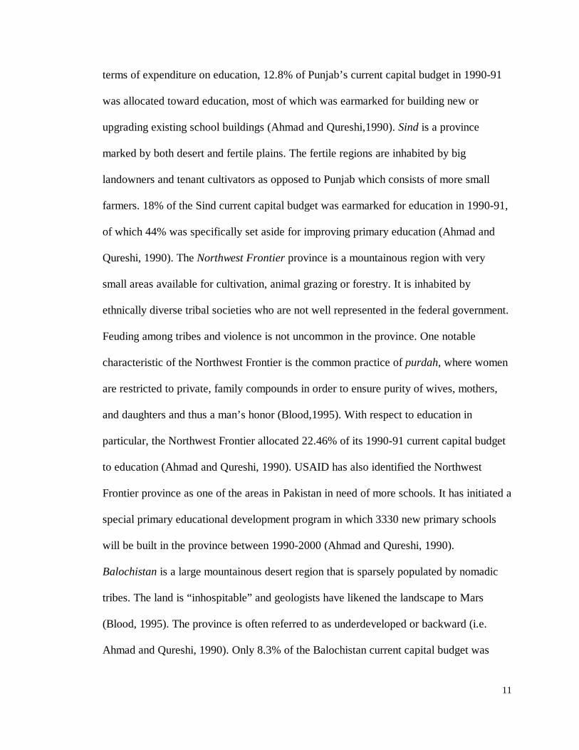
terms of expenditure on education, 12.8% of Punjab’s current capital budget in 1990-91

was allocated toward education, most of which was earmarked for building new or

upgrading existing school buildings (Ahmad and Qureshi,1990). Sind is a province

marked by both desert and fertile plains. The fertile regions are inhabited by big

landowners and tenant cultivators as opposed to Punjab which consists of more small

farmers. 18% of the Sind current capital budget was earmarked for education in 1990-91,

of which 44% was specifically set aside for improving primary education (Ahmad and

Qureshi, 1990). The Northwest Frontier province is a mountainous region with very

small areas available for cultivation, animal grazing or forestry. It is inhabited by

ethnically diverse tribal societies who are not well represented in the federal government.

Feuding among tribes and violence is not uncommon in the province. One notable

characteristic of the Northwest Frontier is the common practice of purdah, where women

are restricted to private, family compounds in order to ensure purity of wives, mothers,

and daughters and thus a man’s honor (Blood,1995). With respect to education in

particular, the Northwest Frontier allocated 22.46% of its 1990-91 current capital budget

to education (Ahmad and Qureshi, 1990). USAID has also identified the Northwest

Frontier province as one of the areas in Pakistan in need of more schools. It has initiated a

special primary educational development program in which 3330 new primary schools

will be built in the province between 1990-2000 (Ahmad and Qureshi, 1990).

Balochistan is a large mountainous desert region that is sparsely populated by nomadic

tribes. The land is “inhospitable” and geologists have likened the landscape to Mars

(Blood, 1995). The province is often referred to as underdeveloped or backward (i.e.

Ahmad and Qureshi, 1990). Only 8.3% of the Balochistan current capital budget was

12

allocated to education in 1990-91, the lowest of all four provinces (Ahmad and Qureshi,

1990). Estimates of the educational expenditure per individual ages 5-24 suggests that the

Northwest Frontier province spends the most with.08 rupees/school-age child, followed

by Sind (.06), Punjab (.04) and finally Balochistan (.03).10 Educational outcomes in all

four provinces from the PIHS 1991 are illustrated in Table 2. In general, Punjab exhibits

the highest enrollment rates and mean education levels, while Balochistan has the lowest.

2c. Model Specification and Empirical estimation

Ideally, a researcher analyzing the determinants of schooling would like to

account for the final schooling level an individual attains and know the environment each

lived in when the sequence of schooling decisions were made. Unfortunately, most

surveys provide little information about where the adults in the sample grew up. The

factors which influence adult schooling are therefore unknown (e.g. family income,

community wages, distances to school, etc.). Research that concentrates on the

determinants of child schooling has two advantages. First, using children as the unit of

observation permits the use of information about the current parental, household and

community characteristics, and thus the environment in which the schooling decisions are

made. Second, because many developing countries are experiencing rapid expansions and

structural change in their education systems, birth cohort differences are evident and the

study of current child schooling is most relevant to policy. To use the current generation

10 To approximate province-specific population levels for 1990-91, data from the last available Pakistancensus (1981) was adjusted by the population growth rate for each province from 1972-81 (PakistanStatistical Yearbook, 1994; Statistical Pocketbook of Pakistan, 1995).

13

of children in an analysis of schooling requires that both the censoring of final schooling

for enrolled children and the selection problem arising from sampling home-resident

children be addressed.

Further limitations are imposed by the data. First, surveys measure schooling by

the “years of education attained”. While the desired level of schooling may be

continuous, the researcher only observes education level in discrete (non-negative) year

intervals. Second, there is often a large mass point at zero years of schooling and similar

probability spikes at primary and secondary completion levels where matriculation to the

next level is impeded by fees or entrance examinations.11 Ordinary least squares (OLS)

estimation is thus inappropriate due to the non-negative restriction, the discreteness and

the probability spikes of the schooling variable. Most studies have however used OLS to

estimate the determinants of schooling (for example, Barros and Lam, 1992; Birdsall,

1980;1982;1985; Chernichovsky, 1985; Behrman and Wolfe, 1987; Handa, 1996;

Jamison and Lockheed, 1987; Knight and Shi, 1996; Parish and Willis, 1993; Wolfe and

Behrman, 1984;1986; Case and Deaton, 1996). One recent study by Tansel (1997)

accommodates the spike at zero by estimating a probit for primary, and two-limit Tobits

for secondary and higher education, but the Tobit specification fails to account for the

discreteness of observed schooling in the continuous observed range. Lastly, (to be

developed further in Section 3a), the model employed should account for the right-

censored observations of enrolled students. The estimation strategy that best deals with

the non-negative restriction, the discreteness, the spikes and the right-censoring is the

censored ordered probit model proposed by King and Lillard (1983;1987) and

11 In the PIHS 54% of 15-20 year old girls and 24% of 15-20 year old boys in Pakistan have never attendedschool. Figure 1 suggests that in Pakistan, the distribution of completed schooling has probability spikes at

14

subsequently used by Glewwe and Jacoby (1992), Alderman et al (1995) and Behrman et

al. (1997).

The censored ordered probit framework is estimated in the following way:

Define S* as the desired level of schooling, a continuous variable which depends

linearly upon the observed regressors, x, and a residual term, ε: 12

S* = β'x + ε (2)In practice, we do not observe desired schooling S*. For those individuals who

have finished schooling (uncensored observations), we observe a discrete level of

completed education, S, where

S = 0 if S* ≤ µ0 (3) = 1 if µ < S* = µ1,

= 2 if µ1< S* = µ2, . . . = J if µj− 1= S*.

Thus, the µ’s are threshold parameters which denote a transition from one year of

schooling to the next. For example, the probability that a non-enrolled individual is

observed to have completed two years of school (S=2) is the probability that the value of

the latent schooling attainment function, S*, lies between µ1 and µ2. Under the

assumption that ε is distributed normally, we have

Prob(S=0) = Φ (µ0− β'x) (4)Prob(S=1) = Φ (µ1-β'x) - Φ (µ0-β'x)Prob(S=2) = Φ (µ2-β'x) - Φ (µ1-β'x)...Prob(S=J) = 1- Φ (µj− 1− β'x).

The likelihood function for uncensored observations, Lu, is thus

years 5 and 10 (primary and secondary completion).

15

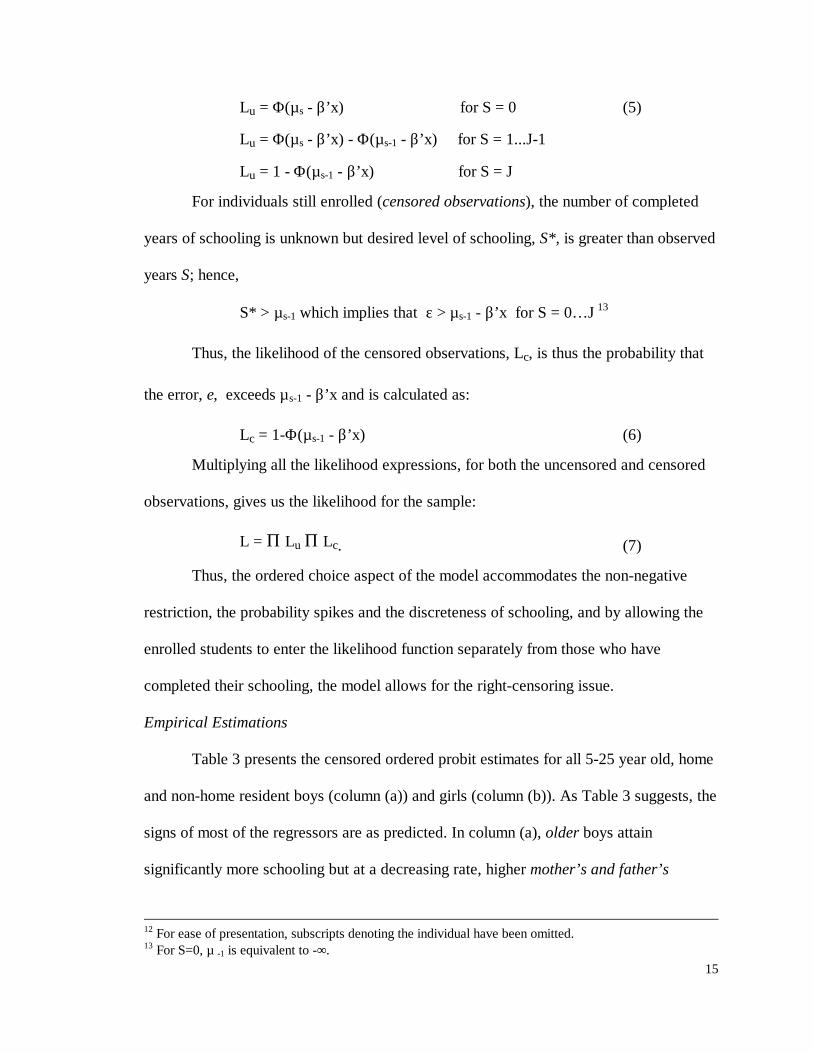
Lu = Φ (µs - β’x) for S = 0 (5)

Lu = Φ (µs - β’x) - Φ (µs-1 - β’x) for S = 1...J-1

Lu = 1 - Φ (µs-1 - β’x) for S = J

For individuals still enrolled (censored observations), the number of completed

years of schooling is unknown but desired level of schooling, S*, is greater than observed

years S; hence,

S* > µs-1 which implies that ε > µs-1 - β’x for S = 0… J 13

Thus, the likelihood of the censored observations, Lc, is thus the probability that

the error, ε, exceeds µs-1 - β’x and is calculated as:

Lc = 1-Φ (µs-1 - β’x) (6)

Multiplying all the likelihood expressions, for both the uncensored and censored

observations, gives us the likelihood for the sample:

L = Π Lu Π Lc. (7)

Thus, the ordered choice aspect of the model accommodates the non-negative

restriction, the probability spikes and the discreteness of schooling, and by allowing the

enrolled students to enter the likelihood function separately from those who have

completed their schooling, the model allows for the right-censoring issue.

Empirical Estimations

Table 3 presents the censored ordered probit estimates for all 5-25 year old, home

and non-home resident boys (column (a)) and girls (column (b)). As Table 3 suggests, the

signs of most of the regressors are as predicted. In column (a), older boys attain

significantly more schooling but at a decreasing rate, higher mother’s and father’s

12 For ease of presentation, subscripts denoting the individual have been omitted.13 For S=0, µ -1 is equivalent to -∞ .

16

education significantly increases the education of their sons, as does higher household

landholdings and property. Being Muslim significantly increases final attainment of boys,

relative to adhering to Christianity or other religious beliefs. Having no sewage disposal

system in the community is significantly associated with less schooling. The distance to

the nearest primary school bears no relation to boys’ years of schooling but the distances

to middle and secondary school are significantly and negatively related to educational

attainment. The average female wage reduces boys’ school attainment while the average

male wage is positively and significantly related to their schooling level. Lastly, relative

to Punjab, boys living in the Northwest Frontier or Balochistan have significantly higher

schooling levels.

Many of the above patterns are evident in the girls sample as well (column (b),

Table 3). Older girls attain significantly more education, at a decreasing rate. Both

mother’s and father’s education are important factors in increasing their daughter’s

education. The value of land and property has a significant and positive effect on girls’

schooling, as does Muslim status and the average male wage. Rural residence has the

expected negative and significant influence on female attainment, as do no sewage

disposal in the community and distances to middle and secondary school. Like boys,

distance to primary school does not appear to affect girls’ schooling.

A few differences between the results for girls and boys deserve emphasis. For

example, while positive and significant for both, the effect of mother’s education is

greater for girls than for boys. Furthermore, for girls, the magnitude of mother’s

education is greater than for father’s education, while the reverse is true for boys. Rural

residence significantly decreases girls’ attainment as expected, but recall it has no effect

17

on boys’ attainment. The lack of sewage disposal in the community is less associated

with the schooling of boys compared to that of girls, although the coefficient is

significant and negative in both samples. The average female wage has no effect on girls’

schooling while it is a significant and negative determinant of boys’ schooling.

Furthermore, the wealth effect on attainment is much larger for girls; the magnitudes of

the coefficients for land and property and the average male wage are two to three times

higher in the girls’ sample than the boys’. Lastly, while none of the province indicators

are significant in the girls’ sample, living in the Northwest Frontier or Balochistan

province (relative to Punjab) is positively associated with schooling attainment for boys.

Figure 1 shows the distribution of schooling attainment in Pakistan for individuals

ages 15-20, by sex. Note the increased frequencies at years 1, 5 and 10 years.

Furthermore, although not shown in Figure 1, 54% of females and 24% of males in this

age group have zero years of education, adding another spike in the distribution. Such

non-linearities suggest that the above censored ordered probit specification is an

improvement over the typical OLS (linear) specification. Figures 2a and 2b plot the

estimated thresholds (µ’s) from the censored ordered probit model for boys and girls

(from columns (a) and (b) in Table 3). The thresholds increase in a non-linear fashion,

with steeper ascents at the end of primary school (year 5) and the end of secondary school

(year 10). The non-linearity is particularly evident in the girls sample, justifying the use

of the non-linear ordered choice framework.

18

Comparison to previous work on schooling in Pakistan

Some of the results above may be compared to previous studies of educational

outcomes in Pakistan. The significant positive association between household income and

schooling outcomes has appeared in several studies; for example, a series of studies using

the International Food Policy Research Institute (IFPRI) 1989 survey of four rural regions

in Pakistan found evidence of the positive impact of household income on schooling

attainment (Alderman et al., 1995, 1996; Behrman et al., 1997) as did the studies by

Burney and Irfan (1991) which utilized the 1979 Population, Labor Force and Migration

national survey and by Sathar and Lloyd (1993) which employed the PIHS 1991.

The relationship between parental education and child schooling is less conclusive

in previous studies of Pakistan. While I found a positive and significant effect for both

mother’s and father’s education on both boys’ and girls’ education, King et al (1986),

using the 1979-80 Asian Marriage surveys, found a clear positive effect of father’s

education on both sexes, but no significant effect of mother’s education on boys’

schooling and a significant effect for girls only in the middle class, urban sub-sample.

This is similar to several studies which used the 1989 IFPRI survey of rural Pakistan.

Alderman et al (1995;1996) and Behrman et al (1997) found no effect of mother’s

primary schooling on child school attainment, although the sample of mothers reporting

any primary education was small. Two of the IFPRI studies found a significant and

positive association between father's schooling and children's education (Alderman et al

1995, Behrman et al, 1997) but a third found no significant association when child's

attainment was conditioned on starting school (Alderman et al, 1996). Burney and Irfan

(1991), using the 1979 Population, Labor Force and Migration survey, found a positive

19

and significant effect of both parent’s education on school enrollments and in general

found father’s education to have a greater effect. Lastly, Sathar and Lloyd (1993), using

the PIHS 1991, showed that whether a mother ever attended school was a positive and

significant predictor of children’s primary school completion while father’s literacy was

unrelated.

The effects of school supply characteristics are similarly inconsistent across

previous studies. Recall that this study found no effect of primary school distance but a

negative and significant effect of middle and secondary school distances on both boys’

and girls’ schooling. In contrast, Alderman et al (1996) found that the distance to primary

school had a surprising positive association with school attainment for those who began

school, yet the distance to middle school was unrelated. Sathar and Lloyd (1993) found

that having a public school less than one kilometer away was unrelated to primary school

completion and had a significant and positive effect on primary school attendance for

rural girls only. Burney and Irfan (1991) found that the presence of a school in the village

had no effect on the probability of enrolling in school. On the other hand, results from

Alderman et al. (1995, 1996) and Sabot (1992) suggest a significant role of school supply

on cognitive achievement, perhaps the most important product of schooling. Using the

rural IFPRI survey of 1989, Alderman et al (1995) in particular show that at least 40

percent of the gender and regional gaps in literacy and numeracy tests are associated with

gender and regional disparities in local school availability.

3. Empirical Issues: Censoring and Sample Selection

The estimation described in Section 2c accounts for right-censoring of enrolled

children and includes children who have already left the home. It is considered the

20

preferred framework. The following sections explore the implications of neglecting these

issues in terms of both censoring and sample selection bias in the estimation of the

demand for child schooling.

3a. Censoring of final attainment for enrolled children

Children who are still enrolled in school pose a potential problem for researchers

since for these children, final attainment is unknown but is greater or equal to current

completed years. Several techniques have been used previously to deal with these right-

censored observations. One approach is to define the samples to include only those above

the age of likely school completion, thus limiting samples to older populations and

throwing away many younger observations (Alderman et al, 1996; Beller and Sin Chung,

1992; Knight and Shi, 1996; Lazear, 1977; Leibowitz, 1974;Tansel, 1997).14 The

elimination of these observations may be less satisfactory for low-income countries

experiencing rapid change in enrollments and attainment. For example, in Pakistan, the

mean education of females ages 15-20 is 3.53 years, while for the female cohort ages 25-

30 it is only 2.03 years, implying that mean education increased nearly 75% in one

decade (PIHS 1991). Also, since many household surveys do not inquire about the

childhood environment of adults, as the minimum age for included observations rises,

14 Lazear (1977) and Knight and Shi (1996) may have introduced some selection bias in their respectivesamples. Lazear used a sample of 1969 US individuals aged 17-27, but excluded those who were attendingschool during the survey or two years previous, an exclusion based on endogenous schooling choice.Knight and Shi (1996) restricted their China sample to individuals age 16 to 30 who completed theireducation, similarly eliminating most of the individuals who are likely to attain the highest levels ofeducation.

21

selective migration out of the parental home may introduce bias in the schooling demand

equation (discussed in Section 3b).15

Studies that include younger children commonly attempt to control for incomplete

schooling by incorporating age and perhaps age squared as covariates in an ordinary least

squares regression of schooling attainment (for example, Anderson et al. 1995; Birdsall,

1985; Behrman and Wolfe, 1987; Handa, 1996, Case and Deaton, 1996). While age may

explain much of the difference in attainment between young, enrolled children and older

individuals who have completed schooling, it does not eliminate the censoring problem

since it does not distinguish between completers and non-completers.16 The usefulness of

age as a control for incomplete schooling is further complicated in low-income countries

where frequent late entry, repetition and sporadic school attendance reduce the power of

age as a predictor of attainment. Research on the determinants of repetition, late entry and

sporadic attendance is sparse, but some evidence suggests the frequency of such

occurrences may be substantial in some low income countries In 1985, the median

repetition rates of primary students were about 16% in low income countries and 11% in

lower middle income countries. Furthermore, the median difference between the student-

years needed per graduate and the years in the primary school system in low-income

countries is a striking four years(where the average primary school cycle in developing

15 If we consider a migrant as anyone that has moved away from their birthplace, then the average age atwhich males (ages 15-25) migrate is 11 years and the average age at which females (ages 15-25) migrate isthirteen years. Approximately 18% of individuals ages 15-25 claimed to be migrants. Overall, 35% ofadults in Pakistan claim to be migrants.16 Consider an analysis on two twelve year old children, one who is enrolled and one who has alreadydropped out. Age as a control does not eliminate the censoring issue since both children are still treatedidentically in the estimation.

22

countries is six years), suggesting the widespread existence of repetition in these

countries (Lockheed and Verspoor, 1991).

Evidence from the PIHS suggests that repetition and late enrollment are frequent

in Pakistan. Table 4 illustrates the percentage of all currently enrolled children in each

grade level, by age in Pakistan. Highlighted are the grade levels for which a student of a

given age is considered to be “on time”. Students falling in categories to the left of those

highlighted are considered “lagging behind”.17 As is clear from Table 4, late entry and

repetition appear to be commonplace in this Pakistani sample - by age eight, 66% of

those enrolled in the sample are below their expected grade. Clearer evidence of late

entry is presented in Figure 3, which displays the proportion enrolled by age and sex. If

all individuals entered at the same age but dropped out at different levels, we would

expect to see maximum enrollment at age 6, with a gradual decline thereafter. Instead,

enrollment rates increase up to age 11 for males and age 9 for females which suggests

that late entry is not uncommon. Thus relying on age as a control for differences in

expected enrollment level may have weak justification.

Another method to deal with unobserved completed schooling has been to

standardize by constructing an ‘age and sex specific schooling index’. For example, “the

ratio of child schooling to the mean schooling of children in the relevant age-sex group”

has been used as the dependent variable in attainment regressions by both Birdsall (1982)

and Wolfe and Behrman (1986). A closely related schooling index is used by Wolfe and

17 Note, I have considered students to be “on-time” for two grade levels at each age group to account forchildren who may have birthdays at the end of the school year. For example, children who were 4 at thestart of the school year would not be enrolled in grade one, but at the time of the survey they may havealready turned five. Having zero years of school is still “on-time” for these children.

23

Behrman (1984) in which child’s schooling is normalized by “eligible years of

schooling” rather than “mean schooling of age/sex cohort”. In a similar vein, Jamison

and Lockheed (1987) use deviations from mean cohort schooling as the dependent

variable in their regression analysis. However, similar to controlling for age as a

covariate, for enrolled students, each of these measures reflects lagging behind or

surpassing one’s classmates in attainment, rather than incomplete schooling spells.

Furthermore, lags at younger ages depress the ratio-form indices more than lags at older

ages. Again, the common occurrence of repetition and late entry suggests that these

relative schooling measures may be a particularly poor choice in low-income countries.

Another approach to the measurement of schooling attainment is done by Barros

and Lam (1993) in which the Brazilian census sample was limited to 14 year olds, an age

group that is required to attend school. Their goal was to estimate the determinants of

schooling attainment of 14 year olds, rather than final attainment. However, it is not

clear whether this indicator of schooling is a good predictor of completed schooling, nor

whether this outcome even enters the household utility function.

Chernichovsky (1985) addressed the censoring issue by separately estimating the

determinants of schooling for enrolled and non-enrolled 6-18 year olds in Botswana, but

without correcting for the selection bias in either set of estimates.

As mentioned in Section 2c, King and Lillard’s (1983; 1987) ordered multinomial

choice model allows complete and incomplete spells to contribute separately to the

likelihood function and consistent and unbiased estimates of the coefficients are

achieved. Their technique which has the most attractive properties, to my knowledge has

24

been used in only a few previous studies (Alderman et al, 1995; Behrman et al, 1997;

Glewwe and Jacoby, 1992).

The implications of failing to properly distinguish between completers and

enrollees are known for OLS estimation, which is the most common form of analysis in

previous studies. It can be shown that if the independent variables are normally

distributed, then not accounting for censored observations and applying OLS introduces a

proportional downward bias in all variable coefficients. Consider the following true

model for completed schooling in years, S*, which is a linear function of some vector of

individual i’s characteristics, Xi:

Si* = β’Xi + εi , where εi ~ N(0,σ2 ). (8)

For children who are no longer in school (and assuming no re-entry), final school

attainment is equal to currently observed grade level (Si* = Si). For children still enrolled

in school, final attainment is not known ---only current grade, Si, is observed. If we

assume children finish the currently enrolled grade, then observed schooling is

necessarily less than or equal to final level (Si ≤ Si*) for enrolled children. Thus, for

those enrolled, final schooling is censored at the individual-specific censoring point, ci.

We have the following censored model:

Completers: Si = β’Xi + εI if Si* < ci (9)

= Si*

Enrollees: Si = ci otherwise

A transformation of the variables allows us to use the results obtained by Greene

(1981) to characterize the bias associated with failing to treat incomplete observations as

censored. Define:

Si = ci - Si , (10)

25

=

i

ii

cX

X and

β

=β1-

so that we have the familiar censored regression model or right-censored Tobit:

Completers: Si = β’Xi + ui if RHS > 0 (11)

Enrollees: Si = 0 otherwise

A closed form solution for the bias of OLS estimation of Si on Xi for all

observations is obtained under the assumption that the independent variables are

distributed normally. Greene (1981) shows that when all observations (both enrolled and

completed) are estimated together by OLS, we can expect that the

plim βOLS = Φ (β’Xi /σ)β. (12)

Thus, sufficiently large values of (β’Xi /σ) imply Φ close to 1 and relatively

small bias, as would occur if Si > 0 occurs frequently or, in other words, most children

have completed schooling. Similarly, small values of (β’Xi /σ) imply Φ close to 0, and

large downward bias, as Si = 0 occurs more frequently and most children are currently

enrolled in school. The main result is that every element of β is estimated with the same

proportional downward bias, and the magnitude of the bias grows with the frequency of

censored observations.

In the present case, the assumption that the conditioning variables are distributed

normally is unrealistic and thus, the expected attenuation bias might not be strictly

proportional in practice. One can still examine the censoring bias by estimating the

schooling equation using both OLS and a right-censored Tobit. I expect smaller

coefficients in the OLS specification relative to the Tobit and more censoring bias in the

estimates for males compared to females since a larger proportion of males are enrolled.18

18 51 percent of boys in the sample are still in school compared to only 34 percent of girls.

26

Table 5 contains OLS and right-censored Tobit estimates of the determinants of

schooling for both home and non-home resident boys and girls, ages 5-25. Results in the

table indicate that Greene’s prediction regarding attenuation bias was generally correct

for both samples. With the exception of a few coefficients which are insignificant, the

OLS parameter estimates are closer to zero when compared to the Tobit coefficients.

Marginal effects for the Tobit estimations are also included in Table 5. The marginal

effects are obtained by scaling the Tobit coefficients by the probability that an

observation is uncensored:

[ ]

σβΦβ=<β=

∂∂ ii

iii

ii X'-c)c*Prob(S

X)XE(S

(13)

Since ci, the censoring point, is only known for enrolled (or censored) individuals,

the proportion of the sample still enrolled is used as a consistent estimator for the

probability that an observation is uncensored:19, 20

=

∂∂

Nnβ

i

ii

X)XE(S

(14)

where n is the number of individuals currently enrolled in school and N is the sample

size.

19 The fact that ci is unknown for completers is not problematic for the empirical estimation of the Tobitcoefficients. It is only necessary to define a dummy variable which indicates that an observation is censored(in this case, enrolled=1,0).20 Note that the latter approximation does not depend upon normality of the independent variables.

27

For the boys sample (column (a), Table 5), a comparison of the OLS and Tobit

estimates reveals that, while positive and significant in both models, mother’s education

becomes noticeably more significant with a marginal effect almost four times as large

with proper treatment of censored students.21 The marginal effect of the distance to

middle school also increases more than seven-fold with the censoring accounted for in the

Tobit.

Column (b) in Table 5 contains the comparison of the OLS and right-censored

Tobit estimates for the sample of girls. First, note that the dummies for the Northwest

Frontier and Balochistan provinces lose significance in the Tobit specification. Also, as

witnessed in the boys’ sample, mother’s education becomes noticeably more significant

in the Tobit framework with a marginal effect more than double its counterpart in the

OLS estimation.

Because the ordered choice specification is the preferred model, it is useful to

compare the estimates of an ordered probit done with and without treating enrolled

children as censored.22 Table 6 presents results of ordered probit and censored ordered

probit estimations of schooling attainment for boys and girls ages 5-25 (both home and

non-home resident). In the boys’ sample (column (a)), when censoring is accounted for in

the censored ordered probit specification, a stronger effect of mother’s education is again

seen - the coefficient increases by a factor of four. The average female wage rate, and the

Northwest Frontier and Balochistan dummies also become significant with proper

treatment of censored observations in the ordered choice framework. There are no

21 Since the cov(βOLS, βTobit) is unknown, it is impossible to make a definitive statement regarding thesignificance of the difference between the two models.22 Since ordered probits do not fit a conditional mean, nothing can be said about the expected censoringbias in the ordered probit framework. The coefficients and marginal effects can still be compared across the

28

changes in significance across coefficients in the girls’ sample (column (b)), yet the

noticeably larger significance of mother’s education in the censored model is again

noted.

A comparison of the marginal effects between the two models is also insightful.23

In both the ordered probit and the censored ordered probit, marginal effects of the

independent variables are computed for each year of schooling. Table 7 displays the

marginal effect of each independent variable on the probability of having zero and five

years of education for both models and for boys and girls separately. For boys, at zero

years of education, the marginal effects are generally similar across the two

specifications, except perhaps for mother’s education, rural residence, the average

female wage and the provincial dummies. By year 5, however, large differences in

magnitude and sign of the marginal effects appear. For girls, again the difference in the

marginal effects of mother’s education and the provincial dummies are seen as early as

zero years of education. While the magnitudes of the marginal effects for 5 years of

schooling begin to diverge in the girls sample, only average female wage changes sign.

A closer look at the differences in the marginal effects is possible. Recall in the

boys’ sample that the coefficient for mother’s education increased by a factor of four

when censoring was accounted for in the ordered probit specification.24 Figure 4 shows

models.23 Again, since the cov(βO.P, βC.O.P.) is unknown, no definitive statement can be made regarding thesignificance of the difference between the two models.24 A similar four-fold increase in the marginal effect was observed with censoring accounted for in theOLS-Tobit comparison for boys.

29

the differences in the marginal effect of mother’s education on boys’ schooling for the

ordered probit and censored ordered probit models. In the censored ordered probit, the

marginal effect of mother’s education on boys’ schooling is much greater than in the

ordered probit at zero years and years 10 and beyond.

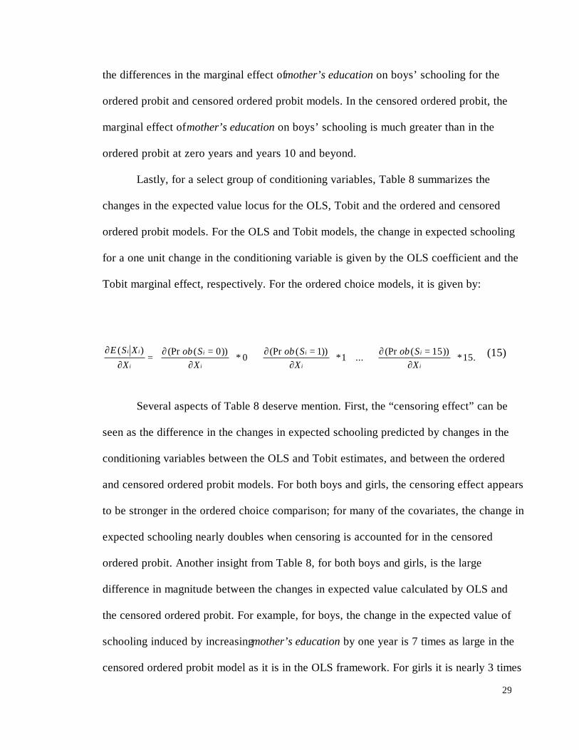
Lastly, for a select group of conditioning variables, Table 8 summarizes the

changes in the expected value locus for the OLS, Tobit and the ordered and censored

ordered probit models. For the OLS and Tobit models, the change in expected schooling

for a one unit change in the conditioning variable is given by the OLS coefficient and the

Tobit marginal effect, respectively. For the ordered choice models, it is given by:

15.*))15((Pr

... 1*))1((Pr

0*))0((Pr)(

∂=∂++

∂=∂+

∂=∂=

∂∂

i

i

i

i

i

i

i

ii

XSob

XSob

XSob

XXSE (15)

Several aspects of Table 8 deserve mention. First, the “censoring effect” can be

seen as the difference in the changes in expected schooling predicted by changes in the

conditioning variables between the OLS and Tobit estimates, and between the ordered

and censored ordered probit models. For both boys and girls, the censoring effect appears

to be stronger in the ordered choice comparison; for many of the covariates, the change in

expected schooling nearly doubles when censoring is accounted for in the censored

ordered probit. Another insight from Table 8, for both boys and girls, is the large

difference in magnitude between the changes in expected value calculated by OLS and

the censored ordered probit. For example, for boys, the change in the expected value of

schooling induced by increasing mother’s education by one year is 7 times as large in the

censored ordered probit model as it is in the OLS framework. For girls it is nearly 3 times

30

as large. Clearly, then, the choice of framework used to estimate schooling attainment has

a large impact on the predictions of the model and the censoring effect appears to be non-

trivial in this case, particularly in the ordered choice specification. The next section

shows that the sample chosen for estimating the demand for schooling will also

significantly influence one’s results.

3b. Selection bias on children currently residing in the home

It is plausible that the decisions to attend school and to remain in the parental

household are related. Table 9 reports probit estimates of the determinants of leaving

home for boys and girls ages 5-25. For boys (column (a)), father’s education, average

male wage, distance to middle school, and the percentage of households which own land

in the community are significantly and negatively associated with leaving home. Rural

family residence significantly increase a male’s probability of leaving home. For girls

(column (b)), age significantly increases the probability of leaving home (at a decreasing

rate), as do percent of males in the community and distance to primary school. Higher

mother’s and father’s education as well as family wealth and average male wages in the

community significantly reduce the likelihood of girls leaving home. Many of these

factors are also significant determinants of educational attainment. Since the factors we

observe influence both the decision to leave home and one’s educational attainment, it

seems likely that the unobservable determinants of both outcomes are also related. The

close relationship between leaving home and educational attainment suggests that home-

resident children may not be a random sample of all children. For example, if the least

able or least motivated children (two unobserved characteristics) tend to leave home at an

earlier age and are less likely to attend advanced schools, then the correlation between the

31

errors in the home leaving and school attainment equations will lead to sample selection

bias when schooling is estimated for home-resident children only. These biases may also

differ by sex, if for example, only the less motivated boys who drop out of school stay at

home, while the less motivated girls who drop out of school leave home and get married.

The following describes the potential bias introduced into the estimation of

schooling demand when children not residing at home are excluded from the sample

(Greene, 1993). Let hi* be a latent variable for residing at home and let wi be the vector

of independent variables determining child i’s decision to stay at home so that:

hi* = γ’wi + ui. (16)

We observe the child staying at home, hi = 1, if hi*>0, otherwise we observe the

child residing elsewhere, hi =0. If we assume that the error term, ui, is distributed

normally with mean zero and unit variance then the probability that the child is observed

living at home is given by

Prob(hi = 1) = Φ (γ’wi), (17)

and the probability that the child is observed not living at home is given by

Prob(hi = 0) = 1 - Φ (γ’wi). (18)

Let Si be the observed years of schooling which is a function of regressors Xi, and

which is observed only if the child resides in the home. Thus we have

Si = β’Xi + εi observed only if hi = 1. (19)

Sample selection bias arises if we believe there exists some correlation among the

errors, ui and εi in equations (16) and (19). For example, if we assume that (u i,ε i) ~

bivariate normal (0, 0, 1, σε, ρ) then ρ is a measure of the correlation among the errors.

The correlation between the two errors will be positive, if for example, being highly

32

motivated or having high genetic ability increases both the probability of staying home

and one’s educational attainment. We can now see the bias introduced by looking at the

mean of the completed education distribution, conditional on the child residing in the

home:

E (Si| hi =1) = β’Xi + ρσελ(γ’wi) where )w'()w'(i

i

γΦγφ=λ (20)

and φ(.) and Φ (.) are the probability and cumulative density functions for the normal

distribution. The conditional mean is thus higher than the unconditional mean if ρ is

positive, and lower if ρ is negative. If not corrected, the effect of sample selection may be

likened to omitted variable bias, where λ(γ’wi) can be viewed as the omitted variable.

Redefining Ψ =ρσε (noting that the sign of Ψ is determined by the sign of ρ) and

simplifying λ(γ’wi) to λ, we have an unbiased specification of the regression model for

the educational attainment of our selected sample:

Si = β’Xi + Ψ λ + νi. (21)

However if we omit λ and simply regress Xi on Si, the estimator becomes

b=β + (X’X)-1X’λΨ + (X’X)-1X’ν. (22)

Thus, even if the included regressors, Xi, are orthogonal to the error, νi, the

existence of a correlation between Xi and λ results in a biased estimate of β, with the

direction of the bias determined by the sign of the second term in (22). Many of the same

regressors are found in both wi and Xi and because λ is a nonlinear transformation of

(γ’wi), a non-zero correlation between Xi and λ is anticipated. Furthermore, the non-zero

33

correlation in the error terms in (16) and (19) (ρ≠0) leads to a non-zero Ψ , further

complicating the bias.

There are few discussions of this form of bias. Some studies had access to

information on all living children and were not faced with the problem (Tansel, 1997;

King and Lillard, 1983, Glewwe and Jacoby, 1992, for example). Most studies do not

mention the possibility of bias nor whether their samples consisted of all children or only

those in residence. Birdsall (1985) is an exception - she acknowledges the possibility of

bias and drops children over the age of 15 to reduce the probability that some children

have left the household. Her approach increases the censoring bias however, as it

increases the proportion of the sample still enrolled. Behrman et al (1997), Birdsall

(1980), Burney and Irfan (1991), Handa (1996), Knight and Shi (1996), and Case and

Deaton (1996) use children resident in the household and do not correct for potential

selection bias. Jamison and Lockheed (1987) use data on household children as well and

re-define children to be any young relative of the household head (including grandchild,

niece and nephew).25

The presence of selection bias can be detected in the PIHS using the data on all

living, home and non-home resident children in the maternal history file. Figure 6 shows

the proportion of children who have left the mother’s household by sex and age. One can

see that the potential for selection bias is greater for girls since by age sixteen, 20% have

already left the home. Table 1 compares the summary statistics for children

25 Such an all-encompassing definition of a household child may complicate the bias since the family’s andhead’s characteristics are attached to both own children and those who have migrated to the relevanthousehold. Furthermore, it is possible that households which “attract” foster children are over-representedin their sample.

34

who have left the home with those who are living with both parents. Children who have

left home are significantly more likely to be female, older, less educated, have less

educated and less wealthy parents, and are more likely to live in rural areas in which

primary and middle schools are farther away. Average male and female wages are also

significantly lower for children who have left home, and they are more likely to come

from the Northwest Frontier province but less likely to come from Balochistan.

A test for selection bias in the estimation of schooling attainment of home-

resident children is done by introducing an additional set of regressors which capture the

effect of residing at home. In addition to the independent variables included in the

previous estimations, a dummy variable for living at home (home) and its interaction with

each of the covariates (e.g. home*age, home*mother’s education, etc.) have been added

to the OLS and censored ordered probit specifications:

Si= β’Xi + γ’homei + δ’(homei*Xi) + εi (23)

A likelihood ratio test of the joint significance of the “home terms” tests for the

existence of selection bias. Under the null hypothesis, γ and δ are jointly not significantly

different from zero, indicating no selection bias exists. Rejection of the null implies the

presence of selection bias and therefore that estimation of the full sample of home and

non-home resident children yields significantly different results from estimation on home

resident children alone. While I consider the censored ordered probit the best

specification, I also perform this exercise using OLS to see if the OLS estimates, which

dominate the literature on schooling attainment, are also prone to selection bias.

35

Appendix B contains the results of the estimation of equation (23) using both

OLS and censored ordered probit specifications, for boys (Table B.1) and girls (Table

B.2) respectively. Table 10 presents the results of the likelihood ratio tests described

earlier. Clearly, for both boys and girls, and for both models, the null hypothesis that the

coefficients on all the “home” terms are jointly equal to zero is rejected. Thus, studies

which omit children who have left the parent’s household are subject to selection bias. If

we assume that the models are estimated with the same level of precision for both boys

and girls, then it appears that the selection bias is more pronounced in the girls' sample,

as evident by the much larger likelihood ratio statistics. This was expected since leaving

home before age 25 is a phenomenon that occurs much more frequently among females

in Pakistan (see Figure 6).

4. Conclusion

When defining a sample for the estimation of the determinants of school

attainment, a researcher faces several obstacles. Adults, whose childhood environments

are rarely characterized in surveys, must be eliminated since the socioeconomic

conditions at the time the schooling choices were made are unknown. Young children,

while perhaps the most relevant sample for current policy insights, are often still enrolled

in school and pose a problem of unknown final attainment. Older children begin to leave

the parental household and thus the home-resident children recorded in most household

surveys become a more select sample. The results of this study suggest that these

problems are not trivial; the methodology employed and the sample one analyzes may

change the results significantly.

36

Tables 11a and 11b summarize the effects of select conditioning variables on

schooling outcomes estimated from the OLS, ordered probit and censored ordered probit

specifications. One can think of the three models as building on each other in complexity;

OLS is the simplest model, the ordered probit framework allows for the discreteness of

the schooling variable and finally, the censored ordered probit model accounts for the

right censoring of enrolled students. For each model, the ceteris paribus change in a

conditioning variable required to move a child from zero to one year of school (Table

11a) or from five to six years of school (Table 11b) can be calculated. This provides a

better indication of the effect of treating schooling years as discrete (by comparing OLS

and ordered probit results) and of treating enrolled students as right-censored (by

comparing ordered and censored ordered probit results).26 For example, according to the

OLS and ordered probit estimates, it takes four additional years of father’s education to

move a boy into grade one while the censored ordered probit results indicate it would

take less than half a year of father's schooling to accomplish the same transition. Moving

a boy from grade 5 to grade 6 requires an additional four years of father's schooling in

OLS, an additional 2.61 years in the ordered probit but less than one additional year in

the censored ordered probit . For girls, a similar pattern exists where in general, the

ordered probit results lie between the OLS and censored ordered probit specifications but

the most pronounced differences exist between the ordered and censored ordered probit

specifications, highlighting the non-trivial censoring effect. Furthermore, the censoring

26 The change in x required to move a child from year j to year j+1, ceteris paribus, is equal to 1/βx forOLS and (µj+1-µj)/βx for the ordered choice models.

37

effect appears to be smaller for the grade 6 transition than the grade 1 transition as

expected, since more individuals are censored at lower grade levels.

This paper has also shown that the sample chosen for the estimation of schooling

demand can alter one’s results. Samples consisting of only home-resident children

introduce significant bias in OLS and censored ordered probit estimates of the demand

for girls’ and boys’ schooling. As expected, since more girls than boys leave home in

Pakistan before age 25, the bias is more problematic in the girls sample.

The preferred framework, a censored ordered probit specification using a sample

of all home and non-home resident children provides some insight into the demand for

child schooling in Pakistan. Parental education is a significant determinant of both boys'

and girls' schooling, with mother's education exerting a larger impact on daughters'

education and father's education influencing more heavily the schooling of sons.

Household wealth is also a major factor in determining children's schooling and its

influence is greater for females. Lastly, while the majority of educational resources in

Pakistan are earmarked for improving access to primary schools, this study suggests that

money would be better spent increasing access to boys' and girls' middle and secondary

schools; distance to primary school does not affect one's attainment whereas distances to

middle and secondary schools are significant determinants of final schooling level.

38

References

Alderman, Harold, Jere Behrman, Shahrukh Khan, David Ross, and Richard Sabot (1995) “Public

Schooling Expenditures in Rural Pakistan: Efficiently Targeting Girls and a Lagging Region” in

Public Spending and the Poor: Theory and Evidence (eds. Kimberly Mead and Dominique van

de Walle). Johns Hopkins University Press for the World Bank.

Alderman, Harold, Jere Behrman, Shahrukh Khan, David Ross, and Richard Sabot (1996).

“Decomposing the Regional Gap in Cognitive Skills in Rural Pakistan” Journal of Asian

Economics 7 (1):49-76.

Ahmad, Raique and Khizr Qureshi, eds. (1990). Budgets of Pakistan: 1990-91. Lahore, Pakistan:

Development Studies Institute.

Amemiya, Takeshi (1985). Advanced Econometrics. Cambridge, MA: Harvard University Press.

Anderson, Kathryn, Elizabeth King and Yan Wang (1995). “Market Returns, Transfers and Demand for

Schooling in Malaysia”. Mimeo.

Barros, Ricardo and David Lam (1993). “Income Inequality, Inequality in Education, and Children’s

Schooling Attainment in Brazil” in Education, Growth, and Inequality in Brazil (eds. Nancy

Birdsall and Richard Sabot).

Becker, Gary (1964). Human Capital. Chicago: University of Chicago Press.

Becker, Gary (1981). A Treatise on the Family. Cambridge, MA: Harvard University Press.

Behrman, Jere and Barbara Wolfe (1987). “Investments in Schooling in Two Generations in Pre-

Revolutionary Nicaragua.” Journal of Development Economics 27:395-419.

Behrman, Jere and Anil Deolalikar (1988). “Health and Nutrition” in Handbook of Development

Economics, Volume 1, (edited by H. Chenery and T.N. Srinivasan).

Behrman, Jere, Andrew Foster, Mark Rosenzweig, Prem Vashishtha (1997). “Women’s Schooling,

Home Teaching and Economic Growth” mimeo.

Behrman, Jere, Shahrukh Khan, David Ross, and Richard Sabot (1997). “School Quality and Cognitive

Achievement Production: A Case Study for Rural Pakistan.” Economics of Education Review

16(2):127-142.

Beller, Andrea and Seung Sin Chung (1992). “Family Structure and Educational Attainment of

Children: effects of remarriage.” Journal of Population Economics (5):39-59.

39

Bilquees, Faiz and Shahnaz Hamid (1989). “Lack of Education and Employment Patterns of Poor

Urban Women in Rawalpindi City” The Pakistan Development Review 28:4 Part II.

Birdsall, Nancy (1980). “A Cost of Siblings: Child Schooling in Urban Columbia” Research in

Population Economics, 2:115-150.

Birdsall, Nancy (1982). “Child Schooling and the Measurement of Living Standards” The World Bank,

LSMS Working Paper no. 14.

Birdsall, Nancy (1985). “Public Inputs and Child Schooling in Brazil” Journal of Development

Economics 18:67-86.

Blood, Peter B., editor(1995). Pakistan: A Country Study. Federal Research Division, Library of

Congress.

Burney, Nadeem and Mohammad Irfan (1991). “Parental Characteristics, Supply of Schools, and Child

School Enrolment in Pakistan” The Pakistan Development Review, 30:1.

Case, Anne and Angus Deaton (1996). “School Quality and Educational Outcomes in South Africa”

Princeton University, mimeo.

Chernichovsky, Dov (1985). “Socioeconomic and Demographic Aspects of School Enrollment and

Attendance in Rural Botswana” Economic Development and Cultural Change 33:319-332.

Cochrane, Susan (1979). “Fertility and Education: what do we really know?” Baltimore: Johns Hopkins

University Press.

Deolalikar, Anil (1993). "Gender Differences in the Returns to Schooling and in Schooling Enrollment

Rates in Indonesia." Journal of Human Resources, 28(4):899-932.

Glewwe, Paul and Hanan Jacoby (1992). “Estimating the Determinants of Cognitive Achievement in

Low-Income Countries: the Case of Ghana.” The World Bank, LSMS Working Paper no. 91.

Greene, W. H.(1981). “On the Asymptotic Bias of the Ordinary Least Squares Estimator of the Tobit

Model,” Econometrica 49:505-513.

Greene, W.H. (1993). Econometric Analysis. New York: MacMillan Publishing Group

Haveman and Wolfe (1984) “Schooling and Economic Well-Being: the role of non-market effects”

Journal of Human Resources 19(3):377-406.

Hamid, Shahnaz (1993). “A Micro Analysis of Demand -side Determinants of Schooling in Urban

Pakistan” The Pakistan Development Review, 32:4,713-23.

40

Handa, Sudhanshu (1996). “Maternal Education and Child Attainment in Jamaica: Testing the

Bargaining Hypothesis” Oxford Bulletin of Economics and Statistics, 58(1):119-137.

Jamison, Dean and Marlaine Lockheed (1987). “Participation in Schooling: Determinants and Learning

Outcomes in Nepal” Economic Development and Cultural Change,35(2):279-306.

King, Elizabeth and Lee Lillard (1983). “Determinants of Schooling Attainment and Enrollment Rates

in the Philippines”, Rand Report # N-1962-AID

King, Elizabeth, Jane R. Peterson, Sri Moertiningsih Adioetomo, Lita J. Domingo, and Sabilia Hassan

Syed (1986). “Change in the Status of Women Across Generations in Asia”, Rand Report #

3399.

King, Elizabeth and Lee Lillard (1987). “Education Policy and Schooling Attainment in Malaysia and

the Philippines.” Economics of Education Review. 6(2):167-181.

Knight, J and Li Shi (1996). “Educational Attainment and the Rural-Urban Divide in China” Oxford

Bulletin of Economics and Statistics, 58(1):83-117.

Lazear, Edward (1977). “Education: Consumption or Production” Journal of Political Economy,

85(3):569-97.

Leibowitz, Arleen (1974). “Home Investments in Children” Journal of Political Economy, 82:s111-

s131.

Lillard, Lee and M. Rebecca Kilburn (1995) "Intergenerational Earnings Linkages: Sons and Daughters

in Malaysia" Rand Report # DRU-1125-NIA.

Lillard, Lee and Robert Willis (1994). "Intergenerational Education Mobility: Effects of Family and

State in Malaysia." Journal of Human Resources, 29(4):1126-66.

Lockheed, Marlaine, Dean Jamison and Lawrence Lau (1980). “Farmer Education and Farmer

Efficiency: A Survey” Economic Development and Cultural Change 29(1):37-76.

Lockheed Marlaine and Adriaan Verspoor (1991). Improving Primary Education in Developing

Countries. New York: Oxford University press.

Mincer, J (1974) Schooling, Experience and Earnings. New York : NBER.

Pakistan Statistical Yearbook. 1994.Federal Bureau of Economic Affairs and Statistics Division.

Government of Pakistan.

41

Planning Commission. Government of Pakistan. 1988. Seventh Five-Year Plan 1988-93 and Perspective

Plan 1988-2003. Volume II.

Parish, William and Robert Willis (1993). “Daughters, Education, and Family Budgets: Taiwan

Experiences” Journal of Human Resources, 29(4):863-898.

Psacharopoulos, G and Maureen Woodhall (1985). Education for Development: An analysis of

Investment Choices. New York: Oxford University Press.

Rosenzweig, Mark (1977).“Farm-Family Schooling Decisions: Determinants of the Quantity and

Quality of Education in Agricultural Populations” Journal of Human Resources, 7(1):71-91.

Rosenzweig, Mark and Robert Evenson (1977). “Fertility, Schooling and the Economic Contribution of

Children in Rural India: an econometric analysis.” Econometrica, 45(5):

Rosenzweig, Mark and Kenneth Wolpin (1988). “Migration Selectivity and the Effects of Public

Programs” Journal of Public Economics, 37(3):265-89.

Sabot, Richard (1992). “Human Capital Accumulation in Post Green Revolution Rural Pakistan: A

Progress Report” The Pakistan Development Review 31(4):449-490.

Sathar, Zeba and Cynthia Lloyd (1993). “Who Gets Primary Schooling in Pakistan: Inequalities Among

and Within Families” The Population Council Working Papers Series- no. 52.

Schultz, T.P. (1988). “Expansion of Public School Expenditures and Enrollments: Intercountry Evidence

on the Effects of Income, Prices, and Population Growth.” Economics of Education Review,

7(2):167-183.

Schultz, T.P. (1988b). “Heterogeneous Preferences and Migration: Self-Selection, Regional Prices and

Programs, and the Behavior of Migrants in Columbia ” Research in Population Economics,

6:163-182.

Schultz, T.P. (1993). “Investments in the Schooling and Health of Women and Men: Quantities and

Returns”. Journal of Human Resources, 29(4):694-734.

Schultz, TW (1960). “Capital Formation by Education” Journal of Political Economy 68(12):571-583.

Schultz TW (1963). The Economic Value of Education. New York: Columbia University Press.

Strauss, John and Duncan Thomas (1995). "Human Resources: Empirical Modeling of Household and

Family Decisions" in Handbook of Development Economics, Volume 3, (edited by J. Behrman

and T.N. Srinivasan).

42

Statistical Pocketbook of Pakistan.1995. Federal Bureau of Economic Affairs and Statistics Division.

Government of Pakistan.

Tansel, Aysit (1997). “School Attainment, Parental Education and Gender in Cote d’Ivoire and Ghana”

Economic Development and Cultural Change, 45(4):825-56.

Thomas, Duncan (1990). “Intrahousehold Resource Allocation: An Inferential Approach,” Journal of

Human Resources, 25:4,635-664.

Thomas, Duncan (1994). “Like Father, Like Son, Like Mother, Like Daughter; Parental Resources and

Child Height” Journal of Human Resources, 29(4):950-988.

Ul Haq, Mahbub (1997). Human Development in South Asia, 1997. Karachi: Oxford University Press.

Wolfe, Barbara and Jere Behrman (1984). “Who is Schooled in Developing Countries? The Roles of

Income, Parental Schooling, Sex, Residence and Family Size.” Economics of Education Review,

3(3):231-245.

Wolfe, Barbara and Jere Behrman (1986). “Child Quantity and Quality in a Developing Country: Family

Background, Endogenous Tastes, and Biological Supply Factors” Economic Development and

Cultural Change 34(4):703-718.

World Development Report 1993: Investing in Health. World Bank. Washington D.C.

Women in Pakistan: An Economic and Social Strategy (1989).World Bank. Washington D.C.

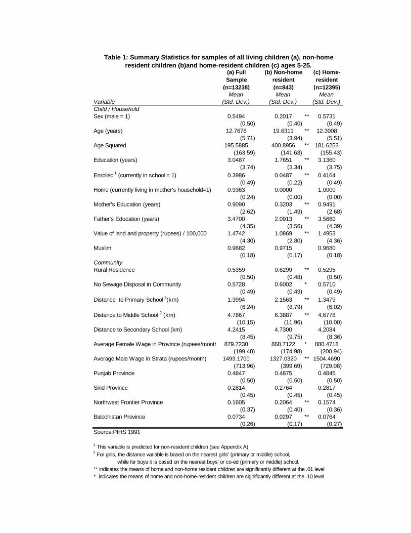
Table 1: Summary Statistics for samples of all living children (a), non-home resident children (b)and home-resident children (c) ages 5-25.

(a) Full Sample

(n=13238)

(b) Non-home resident (n=843)

(c) Home-resident

(n=12395)

VariableMean

(Std. Dev.)Mean

(Std. Dev.)Mean

(Std. Dev.)Child / HouseholdSex (male = 1) 0.5494 0.2017 ** 0.5731

(0.50) (0.40) (0.49)Age (years) 12.7676 19.6311 ** 12.3008

(5.71) (3.94) (5.51)Age Squared 195.5885 400.8956 ** 181.6253

(163.59) (141.63) (155.43)Education (years) 3.0487 1.7651 ** 3.1360

(3.74) (3.34) (3.75)Enrolled 1 (currently in school = 1) 0.3986 0.0487 ** 0.4164

(0.49) (0.22) (0.49)Home (currently living in mother's household=1) 0.9363 0.0000 1.0000

(0.24) (0.00) (0.00)Mother's Education (years) 0.9090 0.3203 ** 0.9491

(2.62) (1.49) (2.68)Father's Education (years) 3.4700 2.0913 ** 3.5660

(4.35) (3.56) (4.39)Value of land and property (rupees) / 100,000 1.4742 1.0869 ** 1.4953

(4.30) (2.80) (4.36)Muslim 0.9682 0.9715 0.9680

(0.18) (0.17) (0.18)CommunityRural Residence 0.5359 0.6299 ** 0.5295

(0.50) (0.48) (0.50)No Sewage Disposal in Community 0.5728 0.6002 * 0.5710

(0.49) (0.49) (0.49)Distance to Primary School 2(km) 1.3994 2.1563 ** 1.3479

(6.24) (8.79) (6.02)Distance to Middle School 2 (km) 4.7867 6.3887 ** 4.6778

(10.15) (11.96) (10.00)Distance to Secondary School (km) 4.2415 4.7300 4.2084

(8.45) (9.75) (8.36)Average Female Wage in Province (rupees/month) 879.7230 868.7122 * 880.4718

(199.40) (174.98) (200.94)Average Male Wage in Strata (rupees/month) 1493.1700 1327.0320 ** 1504.4690

(713.96) (399.69) (729.08)Punjab Province 0.4847 0.4875 0.4845

(0.50) (0.50) (0.50)Sind Province 0.2814 0.2764 0.2817

(0.45) (0.45) (0.45)Northwest Frontier Province 0.1605 0.2064 ** 0.1574

(0.37) (0.40) (0.36)Balochistan Province 0.0734 0.0297 ** 0.0764

(0.26) (0.17) (0.27)Source:PIHS 1991

1 This variable is predicted for non-resident children (see Appendix A)2 For girls, the distance variable is based on the nearest girls' (primary or middle) school, while for boys it is based on the nearest boys' or co-ed (primary or middle) school.** indicates the means of home and non-home resident children are significantly different at the .01 level* indicates the means of home and non-home-resident children are significantly different at the .10 level

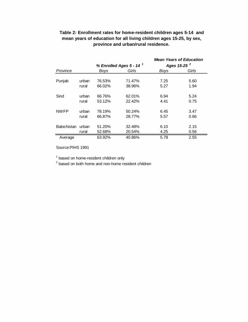
Table 2: Enrollment rates for home-resident children ages 5-14 and mean years of education for all living children ages 15-25, by sex,

province and urban/rural residence.

% Enrolled Ages 5 - 14 1Mean Years of Education

Ages 15-25 2

Province Boys Girls Boys Girls

Punjab urban 76.53% 71.47% 7.25 5.60rural 66.02% 38.96% 5.27 1.94

Sind urban 66.76% 62.01% 6.94 5.24rural 53.12% 22.42% 4.41 0.75

NWFP urban 78.19% 50.24% 6.45 3.47rural 66.87% 28.77% 5.57 0.66

Balochistan urban 51.20% 32.48% 6.10 2.15rural 52.68% 20.54% 4.25 0.56

Average 63.92% 40.86% 5.78 2.55

Source:PIHS 1991

1 based on home-resident children only2 based on both home and non-home resident children

Table 3: Censored ordered probit analysis of the determinants of years of school attainment for all living children ages 5-25, by sex.

(a) (b)Boys Girls

Variables Coefficient (T-Statistic) Coefficient (T-Statistic)Child / HouseholdAge 0.3411 (25.44) 0.2442 (13.99)Age Squared 1 -0.0107 (-23.60) -0.0088 (-14.19)Mother's Education 0.0583 (6.89) 0.1195 (14.28)Father's Education 0.1061 (24.21) 0.0966 (20.55)Value of land and property / 100,000 0.0138 (6.56) 0.0306 (7.54)Muslim 0.3833 (5.00) 0.3087 (2.50)

CommunityRural 0.0651 (1.53) -0.2469 (-4.81)No sewage disposal -0.0866 (-2.16) -0.3741 (-7.75)Dist to Primary -0.0026 (-0.70) -0.0014 (-0.57)Dist to Middle -0.0033 (-1.69) -0.0069 (-3.57)Dist to Secondary -0.0124 (-6.57) -0.0058 (-2.31)Avg Female Wage -0.0068 (-1.85) -0.0013 (-0.29)Avg Male Wage 0.0001 (3.47) 0.0003 (10.48)Sind Province 0.1421 (0.81) -0.2314 (-1.05)NW Frontier Province 2.6365 (1.88) 0.0770 (0.04)Balochistan Province 4.2450 (1.78) -0.1188 (-0.04)Constant 2.7921 (1.00) -1.1577 (-0.33)

Threshold Parameters:µ1 0.0418 (8.35) 0.0315 (6.33)µ2 0.1103 (13.45) 0.0759 (9.40)µ3 0.1829 (17.37) 0.1444 (12.48)µ4 0.2758 (21.54) 0.2462 (15.70)µ5 0.4857 (29.23) 0.5212 (21.69)µ6 0.5790 (32.17) 0.5770 (22.48)µ7 0.7046 (35.54) 0.6275 (23.07)µ8 0.8977 (39.84) 0.8155 (24.62)µ9 1.0013 (41.82) 0.8743 (25.47)µ10 1.4994 (47.01) 1.4121 (26.51)µ11 1.5528 (46.89) 1.4291 (26.51)µ12 1.8828 (41.29) 1.9609 (25.87)µ13 2.0676 (39.29) 2.2195 (23.01)µ14 2.9126 (18.73)Chi-squared(16) 17991.21 10652.08significance level ( 0.0000 ) ( 0.0000 )# Obs 7298 5975Log-likelihood -8082.051 -4902.729Source: PIHS, 1991

1A test that age and age squared are jointly different from zero is significantat the .01 level

Table 4: Proportion of students currently enrolled in each grade, by age

Grade 0 1 2 3 4 5 6 7 8 9 10 11 12 13 14 15Age # obs

5 24 71 3 1 3416 14 65 17 2 1 5667 8 50 29 11 2 7438 3 33 30 21 10 2 8239 1 17 22 23 21 11 3 1 669

10 1 10 14 19 28 17 8 1 1 73011 3 8 15 18 22 21 11 2 53212 3 6 9 14 20 21 18 6 2 1 73613 1 1 5 8 15 22 21 19 5 1 41914 1 1 2 6 11 10 19 21 17 11 44615 1 1 2 3 9 16 24 19 19 5 1 36516 1 1 3 5 8 12 20 34 11 5 1 33217 1 2 5 8 12 29 20 20 3 23418 1 1 2 4 3 8 11 17 14 24 8 5 0 23719 1 1 4 1 9 15 16 31 11 10 0 9120 1 1 1 1 4 2 3 10 9 31 13 21 2 14621 2 2 2 2 11 6 14 26 35 3 6622 1 1 3 11 8 14 18 31 11 7123 3 3 3 10 3 38 34 3 2924 3 7 10 10 34 17 17 2925 7 4 7 7 26 30 19 27

Source: PIHS, 1991Note: Proportions highlighted are those students considered to be "on time" for their age.

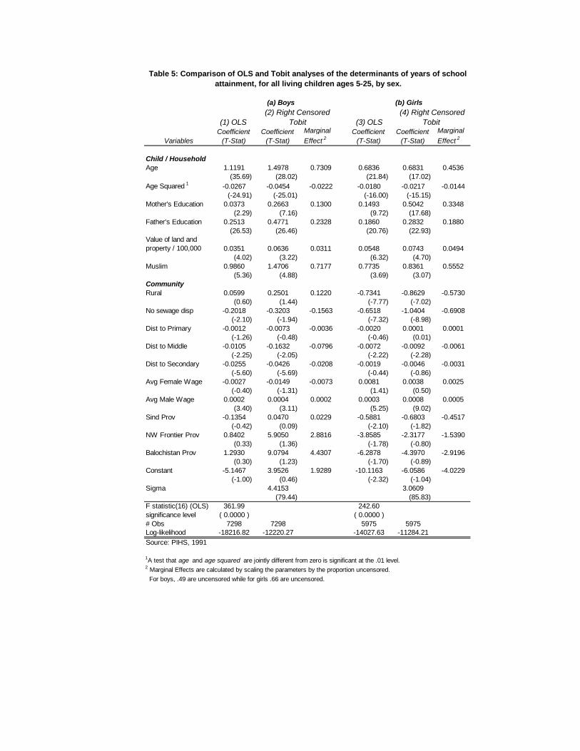
Table 5: Comparison of OLS and Tobit analyses of the determinants of years of school attainment, for all living children ages 5-25, by sex.

(a) Boys (b) Girls

(1) OLS(2) Right Censored

Tobit (3) OLS (4) Right Censored

Tobit

VariablesCoefficient

(T-Stat)Coefficient

(T-Stat)Marginal Effect 2

Coefficient(T-Stat)

Coefficient(T-Stat)

Marginal Effect 2

Child / HouseholdAge 1.1191 1.4978 0.7309 0.6836 0.6831 0.4536

(35.69) (28.02) (21.84) (17.02)Age Squared 1 -0.0267 -0.0454 -0.0222 -0.0180 -0.0217 -0.0144

(-24.91) (-25.01) (-16.00) (-15.15)Mother's Education 0.0373 0.2663 0.1300 0.1493 0.5042 0.3348

(2.29) (7.16) (9.72) (17.68)Father's Education 0.2513 0.4771 0.2328 0.1860 0.2832 0.1880

(26.53) (26.46) (20.76) (22.93)Value of land and property / 100,000 0.0351 0.0636 0.0311 0.0548 0.0743 0.0494

(4.02) (3.22) (6.32) (4.70)Muslim 0.9860 1.4706 0.7177 0.7735 0.8361 0.5552

(5.36) (4.88) (3.69) (3.07)CommunityRural 0.0599 0.2501 0.1220 -0.7341 -0.8629 -0.5730

(0.60) (1.44) (-7.77) (-7.02)No sewage disp -0.2018 -0.3203 -0.1563 -0.6518 -1.0404 -0.6908

(-2.10) (-1.94) (-7.32) (-8.98)Dist to Primary -0.0012 -0.0073 -0.0036 -0.0020 0.0001 0.0001

(-1.26) (-0.48) (-0.46) (0.01)Dist to Middle -0.0105 -0.1632 -0.0796 -0.0072 -0.0092 -0.0061

(-2.25) (-2.05) (-2.22) (-2.28)Dist to Secondary -0.0255 -0.0426 -0.0208 -0.0019 -0.0046 -0.0031

(-5.60) (-5.69) (-0.44) (-0.86)Avg Female Wage -0.0027 -0.0149 -0.0073 0.0081 0.0038 0.0025

(-0.40) (-1.31) (1.41) (0.50)Avg Male Wage 0.0002 0.0004 0.0002 0.0003 0.0008 0.0005

(3.40) (3.11) (5.25) (9.02)Sind Prov -0.1354 0.0470 0.0229 -0.5881 -0.6803 -0.4517

(-0.42) (0.09) (-2.10) (-1.82)NW Frontier Prov 0.8402 5.9050 2.8816 -3.8585 -2.3177 -1.5390

(0.33) (1.36) (-1.78) (-0.80)Balochistan Prov 1.2930 9.0794 4.4307 -6.2878 -4.3970 -2.9196

(0.30) (1.23) (-1.70) (-0.89)Constant -5.1467 3.9526 1.9289 -10.1163 -6.0586 -4.0229

(-1.00) (0.46) (-2.32) (-1.04)Sigma 4.4153 3.0609

(79.44) (85.83)F statistic(16) (OLS) 361.99 242.60significance level ( 0.0000 ) ( 0.0000 )# Obs 7298 7298 5975 5975Log-likelihood -18216.82 -12220.27 -14027.63 -11284.21Source: PIHS, 1991

1A test that age and age squared are jointly different from zero is significant at the .01 level. 2 Marginal Effects are calculated by scaling the parameters by the proportion uncensored. For boys, .49 are uncensored while for girls .66 are uncensored.

Table 6: Comparison of ordered probit and censored ordered probit analyses of the determinants of years of school attainment for all living children ages 5-25, by sex.

(a) (b)Boys Girls

(1) Ordered Probit(2) Censored

Ordered Probit (3) Ordered Probit(4) Censored

Ordered ProbitVariables Coef (T-Stat) Coef (T-Stat) Coef (T-Stat) Coef (T-Stat)Child/HouseholdAge 0.4356 (33.56) 0.3411 (25.44) 0.3328 (19.47) 0.2442 (13.99)Age Squared 1 -0.0110 (-26.87) -0.0107 (-23.60) -0.0095 (-16.63) -0.0088 (-14.19)Mother's Educ 0.0126 (1.74) 0.0583 (6.89) 0.0411 (5.73) 0.1195 (14.28)Father's Educ 0.0900 (22.17) 0.1061 (24.21) 0.0876 (20.81) 0.0966 (20.55)Value of land and property / 100,000 0.0094 (4.18) 0.0138 (6.56) 0.0124 (4.73) 0.0306 (7.54)Muslim 0.4116 (6.90) 0.3833 (5.00) 0.3688 (3.26) 0.3087 (2.50)

CommunityRural 0.0221 (0.61) 0.0651 (1.53) -0.2997 (-6.51) -0.2469 (-4.81)No sewage disp -0.0892 (-2.60) -0.0866 (-2.16) -0.3188 (-7.41) -0.3741 (-7.75)Dist to Primary -0.0040 (-1.29) -0.0026 (-0.70) -0.0024 (-1.07) -0.0014 (-0.57)Dist to Middle -0.0036 (-2.12) -0.0033 (-1.69) -0.0077 (-4.39) -0.0069 (-3.57)Dist to Secondary -0.0121 (-8.06) -0.0124 (-6.57) -0.0055 (-2.53) -0.0058 (-2.31)Avg Fem Wage -0.0019 (-0.66) -0.0068 (-1.85) 0.0015 (0.41) -0.0013 (-0.29)Avg Male Wage 0.0001 (2.80) 0.0001 (3.47) 0.0002 (6.22) 0.0003 (10.48)Sind Province -0.0459 (-0.33) 0.1421 (0.81) -0.2739 (-1.52) -0.2314 (-1.05)NW Frontier 0.6671 (0.60) 2.6365 (1.88) -1.0559 (-0.75) 0.0770 (0.04)Balochistan 1.0474 (0.55) 4.2450 (1.78) -1.6928 (-0.70) -0.1188 (-0.04)Constant -1.9102 (-0.86) 2.7921 (1.00) -4.0242 (-1.42) -1.1577 (-0.33)

Thresholds:µ1 0.3621 (29.01) 0.0418 (8.35) 0.2925 (22.01) 0.0315 (6.33)µ2 0.6199 (39.08) 0.1103 (13.45) 0.5123 (28.98) 0.0759 (9.40)µ3 0.8459 (46.71) 0.1829 (17.37) 0.7221 (34.42) 0.1444 (12.48)µ4 1.0916 (54.52) 0.2758 (21.54) 0.9405 (39.36) 0.2462 (15.70)µ5 1.3953 (63.57) 0.4857 (29.23) 1.2612 (44.68) 0.5212 (21.69)µ6 1.6278 (68.89) 0.5790 (32.17) 1.4380 (46.97) 0.5770 (22.48)µ7 1.8510 (73.28) 0.7046 (35.54) 1.6337 (48.59) 0.6275 (23.07)µ8 2.1201 (77.58) 0.8977 (39.84) 1.8654 (49.78) 0.8155 (24.62)µ9 2.3177 (80.19) 1.0013 (41.82) 2.0384 (50.89) 0.8743 (25.47)µ10 2.8260 (82.31) 1.4994 (47.01) 2.4954 (48.16) 1.4121 (26.51)µ11 2.9848 (83.03) 1.5528 (46.89) 2.6126 (48.02) 1.4291 (26.51)µ12 3.4238 (75.57) 1.8828 (41.29) 3.0634 (43.47) 1.9609 (25.87)µ13 3.7542 (72.03) 2.0676 (39.29) 3.4044 (40.98) 2.2195 (23.01)µ14 4.6100 (40.77) 2.9126 (18.73)Chi-squared(16) 3940.707 17991.21 2741.967 10652.08significance level ( 0.0000 ) ( 0.0000 ) ( 0.0000 ) ( 0.0000 )# Obs 7298 7298 5975 5975Log-likelihood -15107.3 -8082.051 -8857.787 -4902.73Source: PIHS, 1991

1A test that age and age squared are jointly different from zero is significant at the .01 level.

Table 7: Marginal effects on the probability of attaining zero and five years of schooling for ordered probit and censored ordered probit estimations, for all living children ages 5-25, by

sex.

(a) (b)Boys Girls

Education=0 Education=5 Education=0 Education=5

VariablesOrdered Probit

Censored Ordered Probit

Ordered Probit

Censored Ordered Probit

Ordered Probit

Censored Ordered Probit

Ordered Probit

Censored Ordered Probit

Child/HouseholdAge -0.1341 -0.1087 0.0238 -0.0079 -0.1307 -0.0969 0.0239 0.0116Age Squared 0.0034 0.0034 -0.0006 0.0002 0.0038 0.0035 -0.0007 -0.0004Mother's Educ -0.0039 -0.0186 0.0007 -0.0013 -0.0161 -0.0474 0.0030 0.0057Father's Educ -0.0277 -0.0338 0.0049 -0.0025 -0.0344 -0.0383 0.0063 0.0046Value of land and property / 100,000 -0.0029 -0.0044 0.0005 -0.0003 -0.0049 -0.0121 0.0009 0.0014Muslim -0.1268 -0.1221 0.0225 -0.0089 -0.1449 -0.1224 0.0265 0.0146

CommunityRural -0.0068 -0.0207 0.0012 -0.0015 0.1177 0.0979 -0.0222 -0.0117No sewage disp 0.0275 0.0276 -0.0049 0.0020 0.1252 0.1484 -0.0229 -0.0177Dist to Primary 0.0012 0.0008 -0.0002 0.0001 0.0009 0.0006 -0.0002 -0.0001Dist to Middle 0.0011 0.0010 -0.0002 0.0001 0.0030 0.0027 -0.0006 -0.0003Dist to Secondary 0.0038 0.0040 -0.0007 0.0003 0.0022 0.0023 -0.0004 -0.0003Avg Fem Wage 0.0006 0.0022 -0.0001 0.0002 -0.0006 0.0005 0.0001 -0.0001Avg Male Wage 0.0000 0.0000 0.0000 0.0000 -0.0001 -0.0001 0.0000 0.0000Sind Province 0.0141 -0.0453 -0.0025 -0.0033 0.1076 0.0918 -0.0197 -0.0110NW Frontier -0.2054 -0.8400 0.0365 -0.0610 0.4148 -0.0305 -0.0759 0.0036Balochistan -0.3225 -1.3524 0.0573 -0.0983 0.6650 0.0471 -0.1217 -0.0056Constant 0.5882 -0.8895 -0.1046 -0.0646 1.5808 0.4592 -0.2892 -0.0549

1 Calculations based on results reported in Table 1.6.

Boys

OLS 1

Right-Censored

Tobit 1Ordered Probit 2

Censored Ordered Probit 2

Variable

Mother's Education 0.0373 0.1300 0.0394 0.2673

Father's Education 0.2513 0.2328 0.2678 0.4854

Value of land and property / 100,000 0.0351 0.0311 0.0280 0.0632No Sewage Disposal -0.2018 -0.1563 -0.2662 -0.3974Distance to Middle -0.0105 -0.0796 -0.0093 -0.0145

Distance to Secondary -0.0255 -0.0208 -0.0384 -0.0574

Girls

OLS 1

Right-Censored

Tobit 1Ordered Probit 2

Censored Ordered Probit 2

Variable

Mother's Education 0.1493 0.3348 0.0615 0.4446Father's Education 0.1860 0.1880 0.1708 0.3607Value of land and property / 100,000 0.0548 0.0494 0.0241 0.1126Rural -0.7341 -0.5730 -0.5932 -0.9185No Sewage Disposal -0.6518 -0.6908 -0.6316 -1.3902Distance to Middle -0.0072 -0.0061 -0.0144 -0.0246Distance to Secondary -0.0019 -0.0031 -0.0105 -0.0224

1 Results based on Table 1.52 Results based on Table 1.6. The changes in expected schooling for the ordered choice models are obtained by multiplying the year of education by the marginal effect for that year, and then summing across all years.

Table 8: Change in expected schooling for a unit change in select variables for OLS, Tobit, ordered probit, and censored ordered probit specifications, by sex.

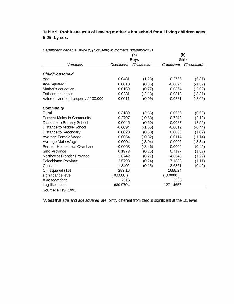
Dependent Variable: AWAY, (Not living in mother's household=1)(a) (b)

Boys GirlsVariables Coefficient (T-statistic) Coefficient (T-statistic)

Child/HouseholdAge 0.0481 (1.28) 0.2766 (6.31)Age Squared 1 0.0010 (0.86) -0.0024 (-1.87)Mother's education 0.0159 (0.77) -0.0374 (-2.02)Father's education -0.0231 (-2.13) -0.0318 (-3.81)Value of land and property / 100,000 0.0011 (0.09) -0.0281 (-2.09)

CommunityRural 0.3189 (2.66) 0.0655 (0.66)Percent Males in Community -0.2797 (-0.63) 0.7243 (2.12)Distance to Primary School 0.0045 (0.50) 0.0087 (2.52)Distance to Middle School -0.0094 (-1.65) -0.0012 (-0.44)Distance to Secondary 0.0020 (0.50) 0.0038 (1.07)Average Female Wage -0.0054 (-0.32) -0.0114 (-1.14)Average Male Wage -0.0004 (-3.04) -0.0002 (-3.34)Percent Households Own Land -0.0063 (-3.46) 0.0006 (0.45)Sind Province 0.1973 (0.25) 0.7197 (1.52)Northwest Frontier Province 1.6742 (0.27) 4.6348 (1.22)Balochistan Province 2.5793 (0.24) 7.1883 (1.11)Constant 1.8402 (0.15) 3.6861 (0.49)Chi-squared (16) 253.16 1655.24significance level ( 0.0000 ) ( 0.0000 )# observations 7316 5993Log-likelihood -680.9704 -1271.4657Source: PIHS, 1991

1A test that age and age squared are jointly different from zero is significant at the .01 level.

Table 9: Probit analysis of leaving mother's household for all living children ages 5-25, by sex.

Boys

Model

OLS (column (1) in Table

1.5)OLS (column (1)

in Table 1B.1)

Censored Ordered Probit

(column (2) in Table 1.6)

Censored Ordered Probit (column (2) in Table 1B.1)

Rhs = β'x

Rhs=β'x + γ'home + δ'(home *x) Rhs = β'x

Rhs=β'x + γ'home + δ'(home *x)

Log-Likelihood -18216.8167 -18141.0324 -8082.051 -8044.419

LR Test Statistic (Chi-squared(17)) 151.5686 75.26

Significance level p=.0000 p=.0000

Girls

Model

OLS (column (3) in Table

1.5)OLS (column (1)

in Table 1B.2)

Censored Ordered Probit

(column (4) in Table 1.6)

Censored Ordered Probit (column (2) in Table 1B.2)

Rhs = β'x

Rhs=β'x + γ'home + δ'(home *x) Rhs = β'x

Rhs=β'x + γ'home + δ'(home *x)

Log likelihood -14027.6301 -13825.8915 -4902.729 -4829.032LR Test Statistic

(Chi-squared(17)) 403.4772 147.394Significance level p=.0000 p=.0000

Table 10: Likelihood ratio tests of joint significance of "Home-resident" variables, by sex.

Table 11a: Change in select independent variables required to move a child from grade 0 to grade 1 for OLS, ordered probit, and censored ordered probit specifications1

Boys Girls

∆x i needed to enter grade 1Mean

(std dev)* OLSOrd

Prob 2

Cens Ord Prob 2

Mean (std dev)* OLS

Ord Prob 2

Cens Ord

Prob 2

Mother's education (yrs) .29 (1.42) 26.85 23.14 0.72 .22 (1.29) 6.69 7.12 0.26

Father's education (yrs) 1.69 (3.18) 3.98 4.02 0.39 2.02 (3.32) 5.38 3.34 0.33

Land and Property/100,000 .87 (3.90) 28.46 38.48 3.03 .84 (2.35) 18.25 23.63 1.03

Dist to Middle (km) 4.06 (8.88) -95.27 -102.87 -12.71 8.62 (13.47) -138.89 -38.04 -4.57Dist to Secondary (km) 5.77 (10.12) -39.26 -29.01 -3.36 5.29 (9.35) insig -53.18 -5.44*means and standard deviations are calculated for individuals with zero years of education

Table 11b: Change in select independent variables required to move a child from grade 5 to grade 6 for OLS, ordered probit, and censored ordered probit specifications1

Boys Girls

∆x i needed to continue from grade 5 to grade 6

Mean (std dev)* OLS

Ord Prob 2

Cens Ord Prob 2

Mean (std dev)* OLS

Ord Prob 2

Cens Ord

Prob 2

Mother's education (yrs) .73 (2.44) 26.85 18.45 1.60 1.34 (2.95) 6.69 4.30 0.47

Father's education (yrs) 3.36 (4.14) 3.98 2.61 0.88 4.80 (4.62) 5.38 2.02 0.58

Land and Property/100,000 1.35 (4.17) 28.46 24.72 6.77 1.52 (3.21) 18.25 14.28 1.82

Dist to Middle (km) 3.08 (7.65) -95.27 -65.27 -28.27 4.50 (10.50) -138.89 -22.99 -8.08

Dist to Secondary (km) 3.05 (6.62) -39.26 -18.63 -7.50 2.81 (6.47) insig -31.98 -10.71*means and standard deviations are calculated for individuals with five years of education

1 Calculations are based on results from Tables 1.5 and 1.62 The change in x required to move a child from year j to year j+1, ceteris paribus, is equal to 1/ βx for OLS and (µj+1-µj)/βx for the ordered choice models.

Source: PIHS, 1991.

Figure 1: Distribution of schooling for individuals ages 15-20, by sex

0

2

4

6

8

10

12

1 2 3 4 5 6 7 8 9 10 11 12 13 14 15

Years of Education

Per

cent

FemalesMales

Figure 2a: Estimated thresholds from censored ordered probit analysis for Boys (taken from Table 3, col (a))

0

0.5

1

1.5

2

2.5

3

3.5

0 1 2 3 4 5 6 7 8 9 10 11 12 13 14

Years of Education

Thre

shol

d V

alue

Figure 2b: Estimated thresholds from censored ordered probit analysis for Girls (taken from Table 3, col (b))

0

0.5

1

1.5

2

2.5

0 1 2 3 4 5 6 7 8 9 10 11 12 13

Years of Education

Thre

shol

d V

alue

Source: PIHS, 1991.

Figure 3: Proportion of home-resident children enrolled in school, by age and sex

0

10

20

30

40

50

60

70

80

90

100

5 6 7 8 9 10 11 12 13 14 15 16 17 18 19 20 21 22 23 24 25

Age

Pro

port

ion

MalesFemales

Source: PIHS, 1991.

Figure 4 : Comparison of marginal effect of mother's education for ordered probit and censored ordered probit specification for boys

-0.02

-0.015

-0.01

-0.005

0

0.005

0.01

0 1 2 3 4 5 6 7 8 9 10 11 12 13 14 15

Years of Education

Mar

gina

l Eff

ect

Ordered ProbitCensored Ordered Probit

Figure 5: Proportion of children who have left mother's household, by age and sex

0

10

20

30

40

50

60

70

80

90

100

5 6 7 8 9 10 11 12 13 14 15 16 17 18 19 20 21 22 23 24 25Age

Pro

port

ion

Males

Females

Appendix A.Table A.1: Summary statistics for non-home resident children with and without

links to parent's household.

(a)Non-home resident children without ties to parents from main

sample

(b)Non-home resident children with ties to

parents through maternity file

n=1582 n=843Mean Mean

Variable (Std. Dev.) (Std. Dev.)Child/HouseholdSex (male=1) 0.1485 0.2017

(0.36) (0.40)Age (years) 20.7541 19.6311

(4.17) (3.94)Education (years) 1.9152 1.7651

(3.52) (3.34)Enrolled (currently in school) 0.0636 0.0487

(0.24) (0.22)Mother Literate 0.0575 0.0657

(0.24) 0.25Father Literate 0.2484 0.2998

(0.43) (0.46)Value of Land and Property (rupees) / 100,000 1.4355 1.0390

(4.18) (2.83)CommunityRural Residence 0.5784 0.6299

(0.49) (0.48)Distance to Primary (km) 2.7933 2.1563

(9.91) (8.79)Distance to Middle (km) 6.6213 6.3887

(11.59) (11.96)Distance to Secondary (km) 4.4277 4.7300

(8.24) (9.75)Average Female Wage (rupees/month) 887.8906 868.7122

(206.27) (174.98)Average Male Wage (rupees/month) 1505.0770 1327.0320

(765.27) (399.69)Punjab Province 0.4437 0.4875

(0.50) (0.50)Sind Province 0.3123 0.2764

(0.46) (0.45)Northwest Frontier Province 0.1618 0.2064

(0.37) (0.40)Balochistan Province 0.0822 0.0297

(0.27) (0.17)Source: PIHS, 1991.Note: The individuals in column (a) are used to predict enrollment rates for individuals in column (b)

Table A.2: Probit results for probability of enrollment for non-home resident boys and girls ages 5-25 (without parental links from main sample and with

a living mother), by sex.

Dependent Variable: Currently enrolled in school(a) (b)

Boys GirlsVariables Coefficient (T-statistic) Coefficient (T-statistic)

Child/HouseholdAge -0.1972 (-7.62) -0.2628 (-8.62)Mother Literate 1.1224 (2.37) 0.9106 (2.72)Father Literate 1.1178 (3.48) 1.1274 (3.89)Value of land and property/100,000 -0.0394 (-1.14) -0.0156 (-0.41)

CommunitySind -1.5142 (-0.19) -0.1846 (-0.42)NWFP -10.5069 (-0.16) -2.6817 (-1.01)Baloch -19.1123 (-0.18) -4.3188 (-0.90)Rural 0.5052 (1.37) 0.0994 (0.30)Distance to Primary 0.0262 (0.56) -0.4338 (-1.63)Distance to Middle -0.0409 (-1.29) 0.0058 (0.35)Distance to Secondary -0.0323 (-0.85) -0.0412 (-1.28)Average Female Wage 0.0273 (0.16) 0.0057 (0.82)Average Male Wage 0.0003 (1.85) 0.0004 (2.63)Constant -18.8968 (-0.15) -2.6583 (-0.50)# obs 237 1349Chi-squared(13) 143.66 (p=0.0000) 216.52 (p=0.0000)Log-likelihood -62.2621 -68.3698

0.687 0.544Source: PIHS, 1991.

Correlation between actual and predicted enrollment

Appendix B.Table B.1: OLS and censored ordered probit analysis of the determinants of

schooling attainment with "home-resident" interactions, for all living boys ages 5-25.

(a) Boys

(1) Ordinary Least Squares(2) Censored Ordered

Probit 1

Variables Coefficient T-Statistic Coefficient T-StatisticChild/Household/CommAge 0.0605 (2.17) -0.0128 (-0.42)Age Squared -0.0001 (-1.62) 0.0002 (0.23)Mother's education -0.0413 (-0.22) -0.0135 (0.18)Father's education 0.5870 (8.51) 0.1763 (6.26)Value of land and property / 100,000 -0.0085 (-0.07) 0.1475 (0.16)Muslim 1.0020 (0.78) 33.8962 (0.00)Rural 0.8738 (1.27) 0.3152 (0.77)No Sewage Disposal 0.3668 (0.62) -0.1439 (-0.35)Distance to Primary School -0.0374 (-0.74) -0.0103 (0.44)Distance to Middle School 0.0157 (0.44) 0.0027 (0.16)Distance to Secondary 0.0311 (1.37) -0.0006 (0.05)Average Female Wage -0.0005 (-1.98) -0.0111 (-0.70)Average Male Wage 0.0042 (3.97) 0.0002 (2.33)Sind Province 20.6300 (1.85) 4.2900 (0.58)Northwest Frontier Province 176.1812 (1.97) 41.6683 (0.69)Balochistan Province 299.6053 (1.97) 32.2752 (0.00)Home -346.1683 (-1.94) -46.7214 (0.00)InteractionsHome*Age 0.0505 (1.80) 0.0472 (1.87)Home*Age Squared -0.0001 (-1.54) -0.0012 (-1.89)Home*Mother's education 0.0811 (0.43) 0.0719 (0.35)Home*Father's education -0.3445 (-4.95) -0.0723 (-2.92)Home*((Land & property) / 100,000) 0.0425 (0.36) -0.1340 (1.19)Home*Muslim -0.0461 (-0.04) -33.5226 (0.00)Home*Rural -0.7619 (-1.10) -0.2371 (-0.49)Home*No Sewage Disposal -0.6048 (-1.01) 0.0534 (0.11)Home*Dist Primary 0.0272 (0.53) 0.0077 (-0.44)Home*Dist Middle -0.0281 (-0.78) -0.0064 (-0.37)Home*Dist Secondary -0.0570 (-2.46) -0.0119 (-0.65)Home*Average Fem Wage 0.0462 (1.97) 0.0104 (0.66)Home*Average Male Wage -0.0004 (-3.79) -0.0001 (-2.26)Home*Sind Province -20.7461 (-1.86) -4.1391 (-0.58)Home*Northwest Frontier Province -175.3528 (-1.96) -39.0297 (-0.66)Home*Balochistan Province -298.3481 (-1.96) -28.0336 (0.00)Constant 341.1031 (1.91) 49.5078 (0.00)F/Chi squared (33) 183.39 18066.48significance level ( 0.0000 ) ( 0.0000 )# observations 7298 7298Log-Likelihood -18141.0324 -8044.419Source: PIHS, 1991.

1 For ease of presentation, the estimated thresholds have been omitted from the table.

Table B.2: OLS and censored ordered probit analysis of the determinants of schooling attainment with "home-resident" interactions, for all living girls

ages 5-25.

(b) Girls

(1) Ordinary Least Squares(2) Censored Ordered

Probit 1

Variables Coefficient T-Statistic Coefficient T-StatisticChild/Household/CommAge -0.0184 (-0.09) -0.3013 (-2.30)Age Squared 0.0019 (0.38) 0.0082 (2.32)Mother's education 0.6631 (8.17) 0.1358 (3.45)Father's education 0.1870 (6.09) 0.0747 (3.91)Value of land and property / 100,000 0.1733 (3.38) 0.0565 (2.35)Muslim 0.4471 (0.75) 0.5852 (0.99)Rural -0.6697 (-2.49) -0.3341 (-1.65)No Sewage Disposal -0.3899 (-1.66) -0.1209 (-0.64)Distance to Primary School -0.0052 (-0.50) -0.0023 (-0.21)Distance to Middle School -0.0071 (-0.84) -0.0116 (-1.19)Distance to Secondary -0.0012 (-0.11) -0.0087 (-0.84)Average Female Wage -0.0340 (-0.50) -0.0081 (-0.20)Average Male Wage 0.0008 (2.70) 0.0004 (2.21)Sind Province 1.6133 (0.51) 0.1928 (0.10)Northwest Frontier Province 12.1315 (0.47) 2.5424 (0.16)Balochistan Province 20.7507 (0.47) 0.9574 (0.00)Home -33.5837 (-0.65) -8.1764 (-0.26)InteractionsHome*Age 0.0604 (3.18) 0.0571 (4.31)Home*Age Squared -0.0139 (-2.66) -0.0180 (-4.81)Home*Mother's education -0.5287 (-6.40) -0.0179 (-0.45)Home*Father's education -0.0125 (-0.39) 0.0229 (1.16)Home*((Land & property)/100,000) -0.1289 (-2.48) -0.0289 (-1.18)Home*Muslim 0.3319 (0.53) -0.2972 (-0.49)Home*Rural 0.0434 (0.15) 0.1229 (0.59)Home*No Sewage Disposal -0.3317 (-1.32) -0.2943 (-1.50)Home*Dist Primary 0.0060 (0.52) 0.0018 (0.17)Home*Dist Middle -0.0014 (-0.15) 0.0045 (0.45)Home*Dist Secondary 0.0022 (0.17) 0.0035 (0.33)Home*Average Fem Wage 0.0004 (0.59) 0.0066 (0.16)Home*Average Male Wage -0.0005 (-1.79) -0.0001 (-0.70)Home*Sind Province -2.0886 (-0.65) -0.4156 (-0.22)Home*Northwest Frontier Province -15.0523 (-0.58) -2.3705 (-0.15)Home*Balochistan Province -25.7406 (-0.59) -0.9743 (0.00)Constant 25.4371 (0.49) 6.9927 (0.23)F/Chi squared (33) 138.06 10799.48significance level ( 0.0000 ) ( 0.0000 )# observations 5975 5975Log-Likelihood -13825.8915 -4829.032Source: PIHS, 1991

1 For ease of presentation, the estimated thresholds have been omitted from the table.

Appendix C. Correlation Matrix

Educ Enrolled HomeMother's educ

Father's educ

Land & Property Rural

No waste disposal

Dist to Prim

Dist to Middle

Dist to Sec

Avg fem wage

Avg male wage Punjab Sind NWFP Baloch

Education 1Enrolled 0.375 1Home 0.090 0.200 1Mother's education 0.243 0.263 0.059 1Father's education 0.329 0.334 0.083 0.509 1Land & Property 0.197 0.121 0.027 0.340 0.265 1Rural -0.216 -0.159 -0.050 -0.267 -0.237 -0.149 1No waste disposal -0.224 -0.155 -0.015 -0.273 -0.236 -0.149 0.640 1Dist to Primary -0.085 -0.068 -0.032 -0.036 -0.056 -0.034 0.080 0.071 1Dist to Middle -0.159 -0.133 -0.041 -0.100 -0.088 -0.074 0.303 0.180 0.313 1Dist to Secondary -0.136 -0.118 -0.015 -0.105 -0.134 -0.075 0.289 0.205 0.206 0.297 1Avg fem wage -0.113 -0.057 0.014 -0.105 -0.128 0.013 -0.028 0.156 0.091 0.123 0.073 1Avg male wage 0.180 0.144 0.061 0.305 0.237 0.265 -0.389 -0.258 -0.022 -0.113 -0.142 0.203 1Punjab 0.092 0.058 -0.001 0.035 0.070 0.010 0.051 -0.033 -0.073 -0.131 -0.031 -0.592 -0.139 1Sind -0.002 -0.021 0.003 0.064 0.030 -0.046 -0.053 -0.137 0.043 0.054 0.012 -0.234 0.050 -0.607 1NWFP -0.069 -0.019 -0.033 -0.082 -0.057 0.065 0.036 0.169 -0.062 0.033 -0.080 0.567 -0.098 -0.424 -0.273 1Baloch -0.075 -0.048 0.044 -0.062 -0.106 -0.031 -0.057 0.061 0.154 0.112 0.150 0.742 0.318 -0.274 -0.176 -0.123 1