Measuring the Cost of Aid Volatility - Brookings · PDF filemeasuring the cost of aid...

MEASURING THE COST OF AID VOLATILITY

Homi Kharas

WOLFENSOHN CENTER FOR DEVELOPMENT

WORKING PAPER 3 | JULY 2008

The Brookings Global Economy and Development working paper series also includes the following titles:

• Wolfensohn Center for Development Working Papers

• Middle East Youth Initiative Working Papers

• Global Health Financing Initiative Working Papers

Learn more at www.brookings.edu/global

Author’s Note:

My thanks to Joshua Hermias for his excellent assistance on this project. I am especially grateful for insightful com-

ments from Nancy Birdsall, Brian Pinto, and the participants of a joint dialogue on aid effectiveness hosted by the

Wolfensohn Center for Development and the OECD Development Centre on June 10, 2008.

Homi Kharas is a Senior Fellow with the Wolfensohn

Center for Development at the Brookings Institution.

CONTENTS

Executive Summary . . . . . . . . . . . . . . . . . . . . . . . . . . . . . . . . . . . . . . . . . . . . . . . . . . . . . . . . . . . . . . . . . . . . .1

Key Findings . . . . . . . . . . . . . . . . . . . . . . . . . . . . . . . . . . . . . . . . . . . . . . . . . . . . . . . . . . . . . . . . . . . . . . .1

Introduction . . . . . . . . . . . . . . . . . . . . . . . . . . . . . . . . . . . . . . . . . . . . . . . . . . . . . . . . . . . . . . . . . . . . . . . . . . 2

Approach . . . . . . . . . . . . . . . . . . . . . . . . . . . . . . . . . . . . . . . . . . . . . . . . . . . . . . . . . . . . . . . . . . . . . . . . . 4

Aid Shocks . . . . . . . . . . . . . . . . . . . . . . . . . . . . . . . . . . . . . . . . . . . . . . . . . . . . . . . . . . . . . . . . . . . . . . . . . . . . 6

Different measures of aid fl ows . . . . . . . . . . . . . . . . . . . . . . . . . . . . . . . . . . . . . . . . . . . . . . . . . . . . . . 6

Aid shocks . . . . . . . . . . . . . . . . . . . . . . . . . . . . . . . . . . . . . . . . . . . . . . . . . . . . . . . . . . . . . . . . . . . . . . . . 7

Aid “shortfalls” and “fat tails” . . . . . . . . . . . . . . . . . . . . . . . . . . . . . . . . . . . . . . . . . . . . . . . . . . . . . . . 7

The Certainty Equivalent Amount of Aid . . . . . . . . . . . . . . . . . . . . . . . . . . . . . . . . . . . . . . . . . . . . . . . . . . 11

The capital asset pricing model applied to aid . . . . . . . . . . . . . . . . . . . . . . . . . . . . . . . . . . . . . . . . . 11

Calculating the deadweight loss from aid volatility . . . . . . . . . . . . . . . . . . . . . . . . . . . . . . . . . . . . 12

Interpreting the deadweight losses from aid volatility . . . . . . . . . . . . . . . . . . . . . . . . . . . . . . . . . 16

Donor contribution to deadweight losses from aid volatility . . . . . . . . . . . . . . . . . . . . . . . . . . . . 19

Aid as Insurance . . . . . . . . . . . . . . . . . . . . . . . . . . . . . . . . . . . . . . . . . . . . . . . . . . . . . . . . . . . . . . . . . . . . . . 21

Concluding Remarks . . . . . . . . . . . . . . . . . . . . . . . . . . . . . . . . . . . . . . . . . . . . . . . . . . . . . . . . . . . . . . . . . . 25

References . . . . . . . . . . . . . . . . . . . . . . . . . . . . . . . . . . . . . . . . . . . . . . . . . . . . . . . . . . . . . . . . . . . . . . . . . . 27

Endnotes . . . . . . . . . . . . . . . . . . . . . . . . . . . . . . . . . . . . . . . . . . . . . . . . . . . . . . . . . . . . . . . . . . . . . . . . . . . . 29

MEASURING THE COST OF AID VOLATILITY 1

MEASURING THE COST OF AID VOLATILITY

Homi Kharas

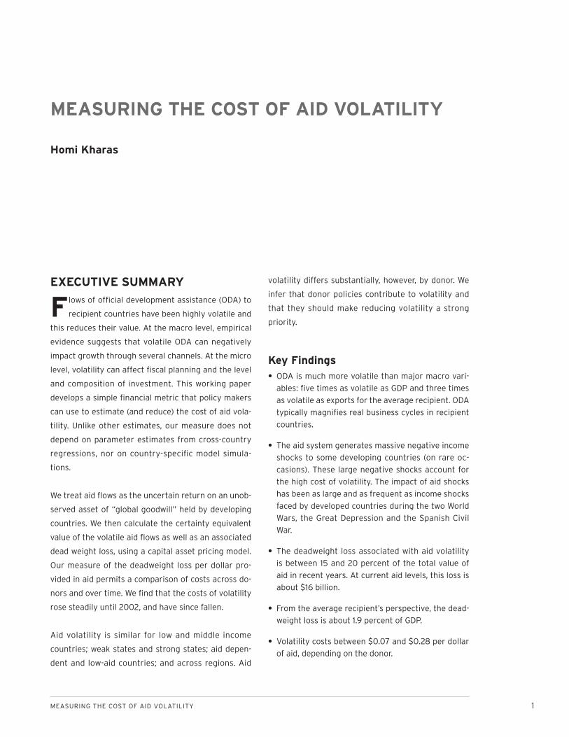
EXECUTIVE SUMMARY

Flows of offi cial development assistance (ODA) to

recipient countries have been highly volatile and

this reduces their value. At the macro level, empirical

evidence suggests that volatile ODA can negatively

impact growth through several channels. At the micro

level, volatility can affect fi scal planning and the level

and composition of investment. This working paper

develops a simple fi nancial metric that policy makers

can use to estimate (and reduce) the cost of aid vola-

tility. Unlike other estimates, our measure does not

depend on parameter estimates from cross-country

regressions, nor on country-specifi c model simula-

tions.

We treat aid fl ows as the uncertain return on an unob-

served asset of “global goodwill” held by developing

countries. We then calculate the certainty equivalent

value of the volatile aid fl ows as well as an associated

dead weight loss, using a capital asset pricing model.

Our measure of the deadweight loss per dollar pro-

vided in aid permits a comparison of costs across do-

nors and over time. We fi nd that the costs of volatility

rose steadily until 2002, and have since fallen.

Aid volatility is similar for low and middle income

countries; weak states and strong states; aid depen-

dent and low-aid countries; and across regions. Aid

volatility differs substantially, however, by donor. We

infer that donor policies contribute to volatility and

that they should make reducing volatility a strong

priority.

Key FindingsODA is much more volatile than major macro vari-

ables: fi ve times as volatile as GDP and three times

as volatile as exports for the average recipient. ODA

typically magnifi es real business cycles in recipient

countries.

The aid system generates massive negative income

shocks to some developing countries (on rare oc-

casions). These large negative shocks account for

the high cost of volatility. The impact of aid shocks

has been as large and as frequent as income shocks

faced by developed countries during the two World

Wars, the Great Depression and the Spanish Civil

War.

The deadweight loss associated with aid volatility

is between 15 and 20 percent of the total value of

aid in recent years. At current aid levels, this loss is

about $16 billion.

From the average recipient’s perspective, the dead-

weight loss is about 1.9 percent of GDP.

Volatility costs between $0.07 and $0.28 per dollar

of aid, depending on the donor.

•

•

•

•

•

2 WOLFENSOHN CENTER FOR DEVELOPMENT

INTRODUCTION

Recent work has shown that aid fl ows to develop-

ing countries are highly volatile, much more so

than other macroeconomic variables such as public

sector revenues, consumption or Gross Domestic

Product (GDP) (Pallage and Robe 2001, Bulir and

Hamann 2006, Fielding and Mavrotas 2005). This

volatility has been of great concern to researchers

and policy makers: it is well known that volatility has

a cost. Bulir and Hamann cite references going back

nearly 40 years decrying aid volatility. More recently,

the Paris Declaration on Aid Effectiveness—an agree-

ment in March 2005 of more than 100 ministers and

senior aid agency offi cials—underscored the determi-

nation of aid donors to make aid more predictable.

Despite this determination, there has not been much

progress in actually reducing aid volatility and some

researchers, like Bulir and Hamann (2006), have ar-

gued that aid volatility has actually become worse

in recent years. This is disappointing as the benefi ts

from reducing volatility and using aid as a smooth-

ing device are thought to be very high. Pallage, Robe

and Berube (2006) conclude that the welfare gain

from improving the timing of aid fl ows could reach 5.5

percent of permanent consumption in aid-recipient

countries. Because aid provides an exogenous instru-

ment for directly infl uencing consumption volatility

in recipient countries, it serves to overcome Lucas’s

(2003) observation that regardless of cost one should

only worry about volatility if there is a mechanism for

reducing it. In this paper we propose a metric for mea-

suring aid volatility with a focus on aid as a smoothing

device for developing countries.

Several studies have documented the cost of aid vola-

tility and the channels through which this operates.1

At a macroeconomic level, aid volatility has been

shown to cause volatility in some aggregate vari-

able such as infl ation (Fielding and Mavrotas 2005),

real exchange rates (Schnabel 2007), or fi scal policy

(Fatas and Mihov 2008). Volatility in these variables,

in turn, has been shown to reduce aggregate growth.

An alternative approach is to directly estimate re-

duced form equations linking volatility in macroeco-

nomic aggregates or aid volatility to lower growth.2

This literature systematically suggests that volatility

is costly, particularly in less developed countries with

weak institutions.

Despite this evidence, aid volatility has not been taken

seriously by policymakers. There are several expla-

nations as to why. First, the policy conclusion from

the finding that high aid volatility reduces growth

is blurred. One can try to minimize aid volatility, or

develop mechanisms to break the link between aid

volatility and the policy variable of choice, or develop

institutions to limit the impact of volatility on growth.

For example, foreign exchange reserve management

could in theory be used to address issues of aid and

exchange rate volatility. Thus, it is hard to establish

that dealing with aid volatility is in fact the priority or

fi rst best response.3

A second problem is that not all aid volatility is bad.

When aid responds to natural disasters, like in the af-

termath of the December 2004 Indian Ocean tsunami,

or the successive droughts in Ethiopia between 2002

and 2004, it can generate volatility in disbursements;

this kind of volatility is regarded as a good thing. In

other words, aid volatility can have a smoothing or

insurance function, depending on whether it is procy-

clical or countercyclical. For some donors, the ability

to reduce aid to corrupt governments or increase aid

to reformist governments after a major confl ict or

crisis is also considered to be a good form of volatility.

Hence differentiating between good and bad volatility

is required.


A third problem is that the nature of evidence on the

costs of aid volatility is often questioned. Some poli-

cymakers dismiss estimates based on cross-country

empirical work because of well-known issues with

low robustness of results. In other cases, costs are

based on simulated parameters for a welfare function

(which can be debated) or on a computable general

equilibrium model with stylized coeffi cients.4 The few

examples of country case studies tend to document

subjective costs, like “diffi culties in planning and bud-

geting,” which are important but hard to quantify.

Donors are increasingly working at the country level

and want an answer to the question “how much does

volatility cost country X.”

In this paper, we try to overcome these problems by

applying a new approach based on a capital asset

pricing model (CAPM) to calculate the deadweight loss

from aid volatility. Such an approach provides a sim-

ple, quantitative measure of the cost of aid volatility in

a framework that differentiates between “good” and

“bad” volatility for each recipient country and that

is decomposable in terms of the contribution of each

donor country to volatility.5 In this way, policymakers

can understand both the aggregate ineffi ciencies of

the current system, the distribution of costs across re-

cipient countries and the contribution of major donors

to these costs.

The remainder of the paper is organized as follows. We

sketch out why a basic CAPM approach, and Sharpe’s

risk-adjusted performance measure, can be usefully

applied to thinking about aid volatility.

The next section looks at the nature of aid shocks. The

use of a Sharpe ratio as the price of risk in applying

the CAPM presumes that a developed capital market

properly values risk. There is no a priori reason to be-

lieve that this should be the case, and this has given

rise to what is known as the “equity premium puzzle.”

Recently, Barro (2006) develops an argument made

by Rietz (1988) that suggests that the risk premium

on US markets can be rationally explained by the fre-

quency and size of major disasters. As Barro notes,

with diminishing marginal utility of consumption, bo-

nanzas do not count nearly as much as disasters for

the pricing of assets and he shows that the frequency

of major disasters is high enough to explain the risk

premium on US stocks. The frequency of major aid

shortfalls, computed in this section, is if anything even

higher than the frequency of major income shortfalls

in a developed country. It is probably reasonable to

believe that developing countries are likely to place

an even higher discount on risk than investors in the

US stock market. Thus, the computed deadweight

losses can be taken as a lower bound of the cost of

aid volatility.

We compute the deadweight loss from aid volatility

and apportion this to each major donor. The cost ap-

pears high, reaching around 15 percent of actual aid

fl ows. This translates into a deadweight loss of around

$16 billion annually in the current system. We also

show that the cost of aid volatility has been growing

over time, although it may have peaked in 2000 and

improved slightly since then.

Section 4 looks at aid as insurance, separating “good”

volatility from “bad” volatility. We look at the role of

aid in smoothing or exaggerating cycles in foreign ex-

change earnings and income.6 Using portfolio valua-

tion approaches, the deadweight loss from aid and the

apportionment of this loss to individual donors is ad-

justed accordingly. Taken together, our results suggest

that aid volatility is a high priority issue, that some

donors are more responsible than others for this, and

that measures to reduce volatility would signifi cantly

enhance the value of aid.


Approach

The approach of this study is to measure the cost

of aid volatility using a Markowitz mean-variance

framework that is the basis of modern fi nance theory.

The CAPM is particularly well suited to valuing a

stream of uncertain cash fl ows and provides a natural

way to value international aid fl ows. In this framework,

we treat aid fl ows as if they are the uncertain returns

on an (unobserved) asset held by a developing coun-

try (its “global goodwill”). The “return” to the asset,

the observed annual fl ow of aid, has a mean and vari-

ance that are summary statistics that suffi ce to mea-

sure the value of the underlying asset. The procedure

is conceptually simple: fi rst convert the uncertain fl ow

of aid into a certainty equivalent amount; second, dis-

count the certainty equivalent amount by the risk-free

interest rate to obtain the value of “global goodwill.”

One advantage of fi nance theory is that it provides a

mechanism for computing the certainty equivalence

which does not require information on the degree

of risk-aversion of the aid recipient country. Instead,

it prices risk using data from international finan-

cial markets. In this paper, we use the price of risk

as determined in markets in the United States—the

so-called Sharpe ratio. The Sharpe ratio—also called

the reward-to-variability ratio—is the premium over

a benchmark risk-free return demanded by investors

per unit of risk associated with a cash-fl ow. Investors

commonly use Sharpe ratios to compute the certainty

equivalence of cash fl ows and derive the value of the

underlying asset.

Sharpe (1966, 1994) developed his ratio to compare

performance between investment managers based

on the risk they took as well as the realized return. He

proposed a simple “risk-adjusted performance mea-

sure” to compare portfolios, equal to the premium of

the return over a risk-free rate, divided by the volatil-

ity of the portfolio, where the volatility is calculated

as the standard deviation of the simple return. In the

same fashion, if aid portfolios have different volatili-

ties, they should have different “returns” to compen-

sate the recipient country.

Once the certainty equivalent amount for aid fl ows are

derived, we can treat the difference between expected

aid receipts and the certainty equivalent amount as

a measure of the “deadweight loss” associated with

aid volatility. That is, we defi ne the deadweight loss

as the avoidable loss that would be eliminated if aid

was stable or perfectly predictable. The deadweight

loss is something that can be removed by a policy

change. It can also be construed as the cost of activi-

ties undertaken by the country to mitigate the effects

of aid volatility. When these deadweight losses are ag-

gregated across all aid recipient countries, we obtain

a measure of the global deadweight loss from aid vola-

tility. Unlike other estimates of the cost of volatility

(that require complex country-by-country modeling

and assumptions about macroeconomic parameters

and behavioral equations) this methodology is simple

and permits a ready comparison about losses across

aid recipient countries.

Another advantage of fi nance theory is that it can

be easily extended to consideration of a portfolio as

well as any single stream of cash fl ows. Each aid re-

cipient country can be thought of as having such a

portfolio—the elements are “goodwill from the USA,”

“goodwill from Japan,” etc. Standard fi nance allows

us to decompose the deadweight loss of aid volatility

into contributions associated with each donor. This

can then be aggregated across countries to obtain

each donor’s contribution to global deadweight losses

from aid volatility. Such a decomposition might be

useful in spurring action to reduce volatility as each

donor can clearly identify the impact of their own


behavior. In fact, this decomposition permits situa-

tions of individual volatility, but collective stability to

arise. Each donor can individually have volatile aid

(perhaps because of its own procedures) but this may

not contribute to any loss if aggregate aid is stable.

The size of the deadweight loss then depends not only

on donor behavior, but also on behavior of all other

donors. If there is coordinated action or herd behavior

(resulting in the so-called donor darlings and donor

orphans), then collective volatility can be accentuated

by multiple donors. If each donor’s volatility stems

from uncorrelated factors like project specifi c issues,

then aggregate volatility can be reduced by multiple

donors and projects.


AID SHOCKS

In considering aid shocks, two questions must be

answered. What is the type of aid being consid-

ered? And how should one measure the “shock?”

Different measures of aid fl ows

The type of aid considered below is infl uenced in part

by the data availability on aid fl ows. Data is drawn

from the Organization for Economic Co-operation and

Development’s Development Assistance Committee

(DAC).7 This is a creditor reporting system, under

which each donor country reports on its aid to differ-

ent countries. The DAC data provide us with aid fl ows

for 53 donor countries and multilateral agencies (like

the International Development Association), cover-

ing 177 recipient countries between 1970 and 2006.

Not all donors lend to all countries, however, and not

all countries are aid recipients in every year. There

are also potentially some points where data is simply

missing. The total number of observations therefore

consists of 110,636 donor-recipient-year points.

The DAC statistics allow us to defi ne aid in a number

of different ways. First, the amount of net Official

Development Assistance (ODA) received by a country

can be determined. This is the broadest measure of

aid, including such diverse items as food aid, humani-

tarian assistance, technical assistance, and debt relief

as well as amounts given for projects and programs in

aid recipient countries. Net ODA is defi ned to include

all transfers with a grant equivalent amount of more

than 25 percent, so it adds together pure grants and

credits on highly concessional terms. It is the headline

number for offi cial aid targets.

The advantage of using net ODA is that it is the most

comprehensive measure of support to a country. The

disadvantage is that it is actually a composite mea-

sure of two different items: gross disbursements less

repayments on past aid credits. But repayment obliga-

tions are known with certainty (bar minor exchange

rate valuation effects). So the variation in net ODA

really comes from a variation in gross disbursements.

This is the second measure we use. Some analysts feel

that donors might adjust their giving in response to

repayment obligations –so-called defensive lending—in

order to maintain a degree of stability in net transfers.

To the extent that this is an accurate portrayal of do-

nor behavior (and there is some evidence to support

this8) then net ODA is to be preferred as a measure of

aid. But if donors do not respond to repayment obliga-

tions then gross disbursements is preferred.

Much of the aid included in net ODA or gross dis-

bursements does not actually involve a cross-border

transaction. For example, technical assistance typi-

cally involves a consulting contract between a donor

agency and a consulting fi rm in its own country. The

aid recipient receives a service (the consulting re-

port), but the valuation of the service is out of its

control. There are no cash fl ows involved. Volatility

in these kinds of transactions may be less important

than volatility in cash that supports development

projects and programs. At the same time, some have

argued that humanitarian assistance should also be

discounted on the grounds that it is “good” volatility.

Following Kharas (2007), we develop a measure of

aid, called country programmable aid (CPA), which ex-

cludes from the total non-cash fl ow items like techni-

The advantage of using net ODA is that it is the most comprehensive measure of support to a country. The disadvantage is that it is actually a composite measure of two different items: gross disbursements less repayments on past aid credits.


cal assistance, debt relief, food aid, and humanitarian

assistance. We also subtract interest payments made,

so as to arrive at a true fi gure of cash fl ow received by

the recipient country. This concept of aid is closest in

spirit to the concept of a “dividend” payout on global

goodwill.

Rather than arbitrarily choosing between these mea-

sures, we report results using all three. While the

magnitudes of the deadweight losses differ, the same

pattern emerges.

Aid shocks

Aid shocks can be best understood as the differ-

ence between aid amounts and some expected value.

Because we are using fi nance techniques, the absolute

amount of aid is used.9 These aid fl ows are obtained in

constant dollar terms. It is now widely recognized that

aid fl ows are non-stationary so it is appropriate to

work in fi rst differences (Bulir and Hamman 2006).

Thus, the basic model is that the change in aid from

donor i to recipient j at time t, Aijt, is driven by a con-

stant term refl ecting the donor-recipient relationship,

aij, and a random error, e

ijt:

(1) ΔAijt = a

ij + e

ijt

Summing this across all donors yields

(2) ΔAjt = a

ij + u

jtΣi

Equation (2) gives the amount of aid each recipient

country receives over time. In essence, this process

assumes that aid has a linear trend, with the trend

estimated separately for each recipient country. It is

then simple to obtain a time series for expected total

aid in each period. Aid shocks are defi ned as the dif-

ference between actual aid fl ows in each period and

the expected value.

Table 1 provides summary information on the volatility

of aid, as measured by the coeffi cient of variation of

the aid shock. For comparison, the table also provides

equivalent statistics for gross domestic product and

export earnings of aid recipient countries. It is clear

that aid is more volatile than these major macroeco-

nomic aggregates. Aid volatility is fi ve to six times as

large as volatility in GDP and three times as large as

export volatility.

It is also interesting to note that the measure of aid

cash fl ows (i.e., CPA) is more volatile than total aid,

despite the fact that the latter includes debt relief and

humanitarian assistance, both of which are thought of

as being highly volatile. The intuition is simple. If aid is

a fi xed aggregate, then more humanitarian assistance

also implies less money for projects and programs.

Thus CPA will also exhibit high volatility when it is a

substitute for humanitarian assistance.

Table 1 also breaks down volatility into a number of aid

recipient sub-groups: geographic region, degree of aid

dependency, income level, and strength of the state.

None of these broad characteristics appears to have

a sizeable impact on aid volatility.10 There is minor

support for the notion that weaker states have more

volatile aid (perhaps because of a higher risk of policy

reversal), but this is not statistically signifi cant.11 There

is no evidence to support the idea that sub-Saharan

Africa, aid dependent countries, or low-income coun-

tries receive a more volatile stream of aid than other

countries.

Aid “shortfalls” and “fat tails”

How big and frequent are negative aid shocks? Recall

that the explanation for high-risk premiums in devel-

oped country stock markets hinges on the idea that

investors care a lot more about very bad outcomes

compared with bonanzas. Thus, high volatility only


has a high cost if the size of the potential shocks is

large.

Figure 1 presents the data on the size of major aid

shortfalls between 1970 and 2006, expressed as a

percentage of recipient country GDP per capita. An

aid shortfall is simply the difference in aid per capita

between two years. We defi ne major aid shortfalls as

those which involve a loss of per capita income of

more than 15 percent, the same criterion as used by

Barro (2006) and it is only these that are shown in

Figure 1. We look at shortfalls over two years, on the

grounds that it may take time between the policy deci-

sion to reduce aid and actual aid fl ows.

For two year aid differences, we fi nd 72 episodes of

large shortfalls out of 4,192 country-year observa-

tions. That is, the probability of an aid shortfall pro-

ducing a negative shock of 15 percent of GDP per

capita or more, has historically been 1.72 percent in

the period 1970-2006. This compares to Barro’s obser-

vation that the risk of a 15 percent decline in real per

capita income in a developed country during the 20th

century was 1.65 percent.12

Barro’s “low probability disaster” scenarios largely

resulted from the two World Wars, the Spanish Civil

War and the Great Depression. Those episodes are

the only ones in the 20th century with falls in per

Sample (mean CV reported)

Gross Disburse-

ments

Net Disburse-

ments

Country Program-mable Aid GDP (lcu)

Exports (US$)

n=177 n=177 n=177 n=157 n=115

All Countries n ≤ 177 0.545 0.586 0.742 0.111 0.220

SSA n ≤ 51 0.531 0.476 0.523 0.110 0.245

LAC n ≤ 41 0.493 0.575 0.696 0.083 0.209

EAP n ≤ 36 0.559 0.657 0.777 0.114 0.266

Aid Dependent (75th percentile) n ≤ 38 0.430 0.389 0.457 0.108 0.266

Aid Dependent (90th percentile) n ≤ 15 0.514 0.494 0.546 0.109 0.315

Non-dependent n ≤ 111 0.537 0.607 0.787 0.116 0.211

Lower Income Countries n ≤ 53 0.553 0.496 0.553 0.110 0.255

Non LIC n ≤ 124 0.541 0.624 0.823 0.111 0.203

Weak States (1st quintile) n ≤ 26 0.748 0.728 0.742 0.132 0.318

Weak States (1st and 2nd quintile) n ≤ 53 0.574 0.542 0.588 0.112 0.255

Strong States n ≤ 73 0.532 0.604 0.809 0.110 0.203

Table 1: Coeffi cient of variation (detrended data, 1970-2005/6)


capita income of more than 15 percent in developed

countries. What is striking about the data is that in the

1970-2006 period, characterized by unprecedented

prosperity and growth in the world, there have been

episodes of equivalent shortfalls in per capita income

in developing countries due solely to reduced aid re-

ceipts. In other words, the aid system has generated

the same negative shocks to per capita income in

per capita incomes in developing countries, and with

more frequency, as the two World Wars and the Great

Depression generated in developed countries.

Table 2 lists the country-year observations of ma-

jor aid shortfalls for net ODA. Twenty-six developing

countries have witnessed at least one major aid short-

fall, and of these 15 countries have had more than one

such episode. More than half are in Africa, and the

remainder are from across the world. Unsurprisingly,

most are small economies. This follows because an aid

shock of this magnitude requires both high volatility

(numerator) and high aid dependence (low denomina-

tor). The broad range of countries experiencing a ma-

jor aid shock, however, suggests that many countries

might realistically be concerned about a major short-

fall at some point in time.13

The frequency of major aid shortfalls is at least as

large as the frequency of major income shortfalls in

developed countries. Barro (2006) argues that such

income collapse episodes are the underlying rationale

for the equity market premium for volatility. If this line

of reasoning is accepted, then it is reasonable to sup-

pose that the discount associated with aid volatility

would be at least as high as the discount for volatility

in developed country equity markets.

Figure 1: Large aid shortfalls, 1970-2006

24

15

10

8

5

34

111

0

5

10

15

20

25

30

0-0.5-1

Net ODA Shortfall (per capita) / GDP per capita

Fre

qu

en

cy


Two Year Difference

% GDP

Recipient Shortfall Count Maximum Shortfall Average Shortfall

Burundi 2 -35.8 -33.9

Cambodia 4 -84.7 -40.9

Cape Verde 1 -25.5 -25.5

Central African Rep. 1 -15.9 -15.9

Chad 1 -31.1 -31.1

Congo, Dem. Rep. 1 -78.6 -78.6

East Timor 2 -45.7 -40.0

Gambia 3 -25.4 -19.6

Guinea-Bissau 8 -47.5 -28.5

Guyana 2 -30.9 -25.2

Kiribati 8 -42.6 -25.5

Liberia 4 -49.8 -35.3

Madagascar 1 -16.3 -16.3

Mali 1 -17.9 -17.9

Marshall Islands 3 -21.0 -19.0

Mauritania 2 -20.9 -18.9

Micronesia, Fed. Sts. 1 -16.9 -16.9

Mozambique 4 -30.3 -22.5

Nicaragua 1 -23.6 -23.6

Rwanda 2 -49.2 -37.9

Sao Tome & Principe 10 -125.6 -35.7

Sierra Leone 1 -15.3 -15.3

Solomon Islands 4 -31.8 -23.8

Suriname 3 -25.1 -21.1

Viet Nam 1 -18.6 -18.6

Zambia 1 -44.6 -44.6

All Large Events 72 -125.6 -28.8

Table 2: Large net ODA shortfalls, 1970-2006


THE CERTAINTY EQUIVALENT AMOUNT OF AID

Consider the following thought experiment. Two

fi nance ministers from aid recipient countries

are comparing their aid fl ows. Each suffers from vola-

tility but they wonder which of their countries’ has the

higher “global goodwill.” They decide to use Sharpe’s

risk adjusted performance measure to assess their

portfolios. They agree to use the international price of

risk as measured on the New York Stock Exchange as

the relevant price for risk as the large adverse shocks

in aid appear to be similar in size and frequency as

the large adverse shocks affecting mature fi nancial

markets. The two ministers each compute their risk-

adjusted aid fl ows to see who is getting the better

deal from donors in terms of risk-adjusted aid fl ows

per capita.

The capital asset pricing model applied to aid

The fi nance ministers would make a calculation based

on a CAPM. The CAPM is a simple mechanism for as-

sociating the required return on an asset with its risk.

The higher the risk, the higher the return required for

an asset to be held in an effi cient portfolio. The CAPM

shows that this relationship is a straight line.

The CAPM can be used to compute the value of the

underlying unobserved asset, “global goodwill” (Gj)

which provides a claim over a dividend flow (the

amount of aid received by country j) in the next pe-

riod. Global goodwill is an asset which does not de-

preciate and in which there is no investment. Its value

remains constant over time if the expected amount

of aid and the variance of aid and the risk free rate

remain constant.

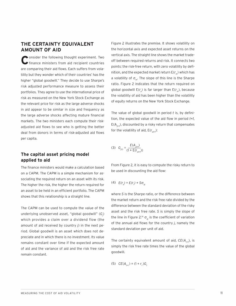
Figure 2 illustrates the premise. It shows volatility on

the horizontal axis and expected asset returns on the

vertical axis. The straight line shows the market trade-

off between required returns and risk. It connects two

points: the risk-free return, with zero volatility by defi -

nition, and the expected market return E(rm) which has

a volatility of σm. The slope of this line is the Sharpe

ratio. Figure 2 indicates that the return required on

global goodwill E(ra) is far larger than E(r

m), because

the volatility of aid has been higher than the volatility

of equity returns on the New York Stock Exchange.

The value of global goodwill in period t is, by defi ni-

tion, the expected value of the aid fl ow in period t+1,

E(Ajt+1

), discounted by a risky return that compensates

for the volatility of aid, E(rat+1

):

(3) Gj(t)

=E(A

jt+1)

(1 + E(rat+1

))

From Figure 2, it is easy to compute the risky return to

be used in discounting the aid fl ow:

(4) E(ra) = E(r

f) + Sσ

aj

where S is the Sharpe ratio, or the difference between

the market return and the risk free rate divided by the

difference between the standard deviation of the risky

asset and the risk free rate. S is simply the slope of

the line in Figure 2.14 σaj is the coeffi cient of variation

of the annual aid fl ows for the country j, namely the

standard deviation per unit of aid.

The certainty equivalent amount of aid, CE(At+1

), is

simply the risk free rate times the value of the global

goodwill.

(5) CE(At+1

) = (1 + rf )G

t


The deadweight loss (DWLt) suffered by the aid recipi-

ent country is defi ned to be the difference between

the expected aid fl ow and the certainty equivalent

amount.

(6) DWLjt = E(A

jt) - CE(A

jt) = E(A

jt) ( )Sσ

aj

1 + rft + Sσ

aj

Equation (6) gives a simple way of computing the

deadweight loss in each period t for each country j.

It shows that the discount between expected aid and

its certainty equivalent amount depends on three key

variables. The discount gets larger as the coeffi cient

of variation of the aid fl ows goes up, as the market

price of risk (the Sharpe ratio) goes up and as the real

risk free interest rate falls.

Calculating the deadweight loss from aid volatility

Equation (3) is a basic formula for computing global

goodwill. For each aid recipient country j we can com-

pute the expected level of aid [based on the trend-

line derived from equation (2)]. The Sharpe ratio is

calculated using the equity returns on the S&P 500

(dividends plus capital gains) and the annualized six

month US Treasury bill rate. Both of these are defl ated

with the US Consumer Price Index (CPI) to obtain val-

ues in real terms. The Sharpe ratio for 1970-2006 is

.388. The mean difference between the equity return

and the risk free return over the period is 6.4 percent.

We have computed the Sharpe ratio for the same time

period as the aid data, namely 1970-2006. Many other

analysts use a Sharpe ratio for the post-WWII period

which is slightly higher than our estimates. If any-

Asset Returns and Risk

Volatility

Ret

urn

σm σa

E(rm )

E(r a)

E(r f )

Figure 2: Asset returns and risk


thing, our procedure biases the estimated deadweight

losses downwards.

Global goodwill for 2002-2006 is shown in Figure 3.

For each country, the expected aid plus or minus one

standard deviation (truncated at zero) is shown. Two

small economies—Cape Verde and the Palestinian

areas—clearly receive higher amounts of aid than

others, with only modest uncertainty. Other high aid

recipient countries also seem to have high volatility.

But there is no simple relationship to identify clearly

which countries have the greatest global goodwill. For

many country pairs there is a trade-off between the

amount of aid and the degree of volatility.

To measure the cost of aid volatility more specifi cally,

we can use Equation (6) to compute the deadweight

loss in constant dollars for each aid recipient country

for each year. These absolute amounts are summed

across recipient countries to give the global dead-

weight loss per year, and divided by total aid for that

year to give the ratio of the deadweight loss to actual

aid for the world as a whole.

The procedure is repeated for each of the three mea-

sures of aid discussed in section 2. The results are

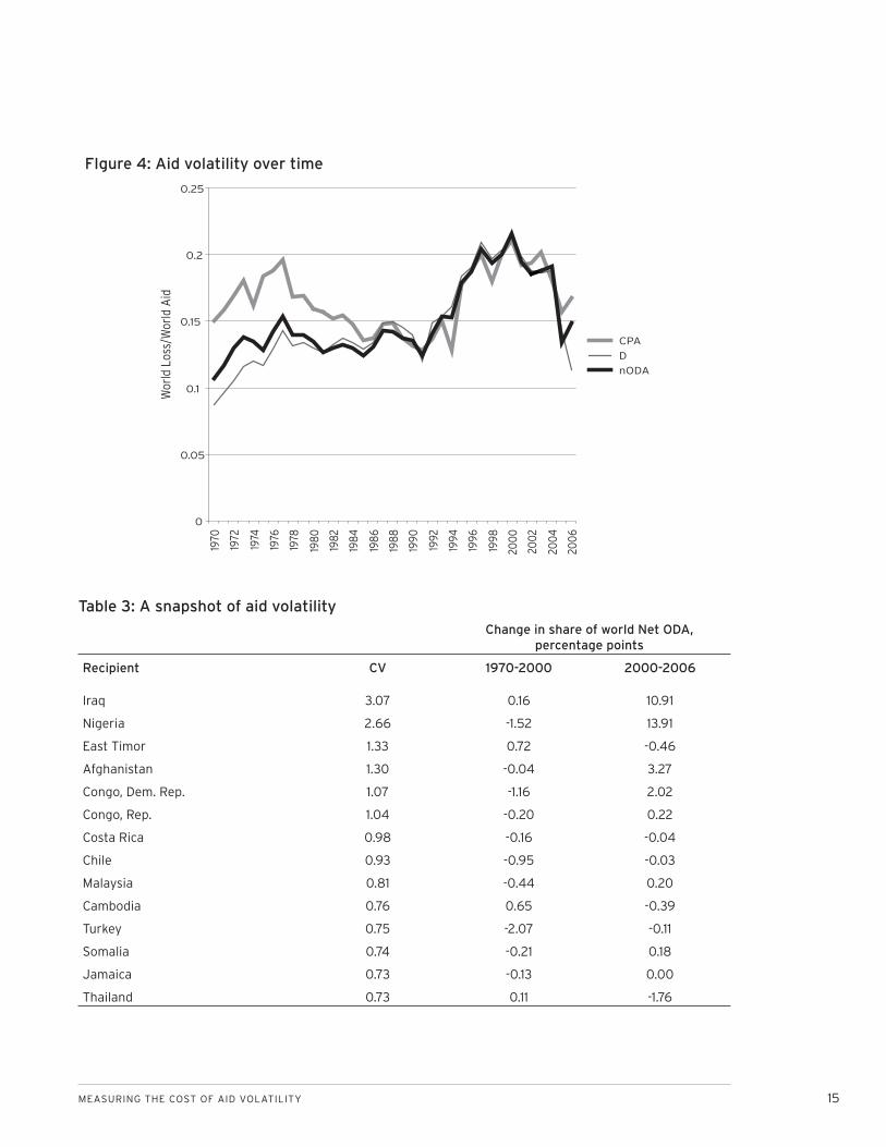
graphically depicted in Figure 4. This aggregation

procedure is equivalent to one which weights each

country-specifi c deadweight loss by the distribution of

aid across countries to get a global total. Thus, if more

aid is channeled towards countries which historically

have had relatively stable aid fl ows, then the global

deadweight loss will decline, and vice versa.

Figure 4 shows that deadweight losses are high, run-

ning between 15 and 20 percent since 1995. Losses

grew steadily from 1970 until about the year 2000.15

They then stabilized at a high level but do appear to

have fallen in the last two years. This cannot be at-

tributed to a fall in the real risk free rate—that has re-

mained at about its long-run average level in the last

few years, and was the same in 2006 as in 1970. Nor

can it be attributed to aid fl ows shifting towards coun-

tries where aid has historically been more volatile;

with some important exceptions, like Iraq, East Timor

and Cambodia, the aid share of countries with the

greatest volatility in aid actually fell between 1970 and

2000 (Table 3). Instead, the rise in deadweight losses

as a share of aid refl ects the movement of aggregate

aid volumes themselves, the denominator in the ra-

tio. When actual aid falls, as it did between 1985 and

2000, the ratio of deadweight losses to aid rose, and

when aggregate aid went up as it has recently done in

2005 and 2006, the ratio fell.

Table 3 shows the changing share in global aid of

countries where aid has been most volatile. It includes

aid recipients, like Iraq, Afghanistan and Cambodia

which are receiving substantially more assistance

than in 1970. But it also includes recipients like Turkey,

Chile and Malaysia where aid volatility has come from

sharply reduced fl ows as these countries came closer

to graduation from development assistance. In be-

tween there are a number of African countries, which

historically have had high aid volatility. The second

and third columns in Table 3 show the change in the

country’s share of aid between 1970 and 2000, the

period during which the measure of computed dead-

weight losses grew, and between 2000 and 2006,

when deadweight losses as a percent of aid fell.

Table 4 presents deadweight losses according to dif-

ferent country groupings as a share of each country’s

GDP. Recall that aid volatility between these country

groupings did not show any marked differences in

terms of recipient country characteristics (Table 1).

But because countries receive different amounts of

aid, the impact of the deadweight losses from aid vola-


0

100

200

300

400

Gpercapita,US$

EthiopiaMorocco

KenyaTogo

MauritiusCambodia

EgyptGuatemala

AfghanistanTunisia

AzerbaijanCroatia

JamaicaSwaziland

ChadTajikistan

ZimbabweSriLanka

CentralAfricanRep.Niger

BurundiMadagascar

Coted'IvoireGuinea

MoldovaSomaliaUganda

TanzaniaAngola

CameroonGhana

HaitiLaos

BurkinaFasoGambia

SurinameBenin

MalawiBotswana

ElSalvadorGabon

SierraLeoneLesotho

SloveniaLiberia

KyrgyzRepublicPapuaNewGuinea

MaliRwanda

FijiCongo,Rep.

ComorosEritrea

SenegalIraq

GeorgiaLebanon

BelizeMozambique

EquatorialGuineaGuinea-Bissau

ArmeniaHonduras

NamibiaZambia

MongoliaBolivia

AlbaniaMauritania

JordanMaldives

EastTimorDjibouti

SerbiaBhutan

NicaraguaBosnia-Herzegovina

GuyanaSolomonIslands

CapeVerdePalestinianAdmin.Areas

Fig

ure

3: G

lob

al g

oo

dw

ill (

G)

pe

r ca

pit

a, 2

00

2-2

00

6


FIgure 4: Aid volatility over time

0

0.05

0.1

0.15

0.2

0.25

1970

1972

1974

1976

1978

1980

1982

1984

1986

1988

1990

1992

1994

1996

1998

200

0

2002

200

4

200

6

Wor

ld L

oss/

Wor

ld A

id

CPA

D

nODA

Change in share of world Net ODA, percentage points

Recipient CV 1970-2000 2000-2006

Iraq 3.07 0.16 10.91

Nigeria 2.66 -1.52 13.91

East Timor 1.33 0.72 -0.46

Afghanistan 1.30 -0.04 3.27

Congo, Dem. Rep. 1.07 -1.16 2.02

Congo, Rep. 1.04 -0.20 0.22

Costa Rica 0.98 -0.16 -0.04

Chile 0.93 -0.95 -0.03

Malaysia 0.81 -0.44 0.20

Cambodia 0.76 0.65 -0.39

Turkey 0.75 -2.07 -0.11

Somalia 0.74 -0.21 0.18

Jamaica 0.73 -0.13 0.00

Thailand 0.73 0.11 -1.76

Table 3: A snapshot of aid volatility


tility in terms of their GDP does differ signifi cantly.

On average, our results suggest that countries lose

about 2 percent of GDP because of aid volatility. But

sub-Saharan African countries and small Pacifi c island

economies are much more sensitive to volatility be-

cause of low levels of GDP and high aid dependency.

For the most aid dependent countries, the losses total

almost 7 percent of GDP. Low income countries and

weak states also have much higher losses from aid

volatility.

Interpreting the deadweight losses from aid volatility

The deadweight losses computed above are fi nancial

and hypothetical in that no actual market transac-

tions are taking place, so we do not observe any

values for “global goodwill” that would permit us to

compute deadweight losses directly. The computa-

tions refl ect comparisons of aid portfolios. But would

a fi nance minister really take less aid totals in return

for reduced volatility? The answer is probably “yes.”

Countries incur substantial real costs from volatility

so welfare could be raised by accepting a smaller total

amount in return for lower volatility.

To see how deadweight losses manifest themselves

in the real world, it is useful to make an analogy to

corporate fi nance. There, it is common to analyze the

problems faced by a fi rm raising fi nances for invest-

ment. Typically, such analysis focuses on the transac-

tion costs of raising money and the uncertainty as to

how much money needs to be raised. If there were no

transaction costs to raising money, fi rms would sim-

Table 4: Dead weight loss as percent GDP, 1970-2006

Average DWL as percent GDP, 1970-2006

Sample nODA D CPA

All Countries 1.92 1.78 1.12

SSA 2.38 3.00 1.69

LAC 0.59 0.68 0.45

EAP 2.70 2.69 2.00

Aid Dependent (75th percentile) 3.98 4.46 2.90

Aid Dependent (90th percentile) 6.60 6.92 4.79

Non-dependent 0.74 0.86 0.51

Lower Income Countries 2.64 3.23 1.85

Non-LIC 1.04 1.07 0.76

Weak States (1st quintile) 2.54 2.88 1.63

Weak States (1st and 2nd quintile) 1.92 2.22 1.33

Strong States 1.19 1.31 0.90


ply wait to see what they needed and then raise that

amount. In practice they do not do this because there

are fi xed costs of negotiating with bankers so they

want to minimize the number of transactions. This

gives rise to a decision to maintain fi nancial slack, or

to preserve a certain amount of liquidity by raising

resources even before they are required. These idle

resources have an opportunity cost that, coupled with

the transaction costs of raising money, becomes a

deadweight loss for the fi rm.

In the case of a country, many of the same issues

arise. The fi nancial planning problem can be thought

of as a two-stage process (Martin and Morgan 1988).

In the fi rst stage, there is an evaluation of how much

money will be required in the next period. In the sec-

ond stage, a decision is made about how much to fi -

nance in the current period and how much to fi nance

in the next period. The decision to pre-fi nance in the

initial period is driven by the desire to minimize trans-

action costs in fi nancing and to give a signal about

fi rms’ investment opportunities. Optimum fi rm fi nanc-

ing behavior can best be interpreted as a decision

to smooth the amount of fi nancing needed so as to

minimize the need to negotiate with additional lend-

ers. The decision is also driven in part because the

signal associated with deviating from a fi nancial plan

is mixed. It can be positive if it refl ects the emergence

of good new investment opportunities; or it can be

negative if it refl ects a shortfall of expected revenues.

The combination of these effects pushes a fi rm (or a

fi nance minister) to develop a predictable fi nancing

plan, even if that entails some real costs compared to

the “fi nance-as-you-go” alternative.16

For a developing country, aid can be uncoordinated

and fragmented. Donors support one sector for a

year and then move towards a different sector. They

are unaware of each others’ operations and often du-

plicate analytical work. The whole system produces

volatility, waste and overlap of activities because of

an inability to predict and plan resource fl ows over the

medium term.

Note that in this model the deadweight losses depend

on transaction costs in the market for fi nance as well

as on uncertainty over the required finance. This

theme is further developed by Aghion et al. (2005). In

that model, there are two types of investment: short-

term investment which generates output relatively

fast; and long-term investment which contributes

more to productivity growth but which carries the

risk that it will be interrupted by an exogenous credit

shock. When long-term investment is interrupted, it

produces a zero return. In such a world, Aghion et al.

show that volatility in domestic liquidity results in a

change in the composition of domestic investment

away from growth-enhancing long-term investment,

and that this effect is largest when domestic fi nancial

markets are less developed. As most of the countries

in our “high aid shock” cases indeed have rudimen-

tary domestic fi nancial markets, the deadweight loss

due to aid volatility can be ascribed to sub-optimal de-

cisions being made in the composition of investment

due to risk-aversion by investors. A fi nance minister

would care about such losses.

Other channels for deadweight losses from aid vola-

tility have also been proposed. Because aid is often

linked with fi scal spending (indeed, much aid is dis-

bursed only after budget expenditures have actually

been made), volatility in aid is linked with volatility in

fi scal spending and hence with volatility in the real ex-

change rate. Real exchange rate volatility, in turn, has

been linked to lower growth by Schnabel (2007) and

Optimum fi rm fi nancing behavior can best be interpreted as a decision to smooth the amount of fi nancing needed so as to minimize the need to negotiate with additional lenders.


by Tressel and Prati (2006), presumably through the

impact on behavior of exporters.

Fatas and Mihov (2008) present evidence that coun-

tries where governments extensively use discretion-

ary fiscal policy experience lower growth. To the

extent that aid volatility responds to and facilitates

such discretionary fi scal policy, it directly contributes

to a loss. For example, many studies have documented

the presence of a political electoral cycle in determin-

ing changes in discretionary fi scal spending.17 Aid can

be used to amplify this kind of opportunistic, non-

economic behavior and the deadweight loss comes

from such “political spending.” In this literature, the

likelihood of such political opportunism rises when the

benefi ts from staying in power rise (when economic

rents are high, for example) and when there are few

institutional checks and balances. Such a scenario

is likely to be the case in aid dependent low-income

countries.

When aid takes the form of a concessional credit

(rather than a grant), then there can be an additional

deadweight loss associated with excessive debt build-

up. Persson and Tabellini (2001) argue that excessive

spending can result when the costs of debt are not

fully internalized by the authorities who may have a

short time horizon. The deadweight losses again arise

from ineffi cient spending.

To summarize this discussion, the deadweight losses

from aid volatility are observed directly in the actions

taken to mitigate such losses. They can accrue in

the form of high costs of fi nancial management, lost

“good” investment opportunities and a sub-optimal

composition of investment, accommodation of non-

economic policies which are detrimental to long-term

growth, the amplifi cation of real business cycles, and

other elements of ineffi cient public spending. From

the perspective of a country and of the welfare of its

citizens, there appears to be a substantial body of

empirical literature suggesting that these deadweight

losses are substantial. Just as many fi rms try to se-

curitize their revenue streams to obtain predictable

fi nancing for investors, so countries would perhaps

want to securitize aid receipts and generate more pre-

dictability if this option was made available.

It must be emphasized that the welfare losses de-

scribed above are not the welfare losses associated

with a simple constant relative risk aversion utility

function. They are far higher because they involve

changes in intertemporal choices by fi rms and indi-

viduals when faced with uncertainty. This is consistent

with the ideas put forward by behavioral economists

that suggest there is an asymmetry in gains and

losses that is much higher than what can be derived

from any reasonable parameters for risk aversion in a

conventional constant relative risk aversion utility.18 As

Rabin (2002, p.9) notes: “the sensation of loss relative

to status quo looms very large relative to gains”. He

cites experiments indicating the existence of a signifi -

cant endowment effect, namely that when something

is taken away it is more highly valued than the ben-

efi t when it is fi rst received. Other experiments sug-

gest reference-based utility—that people care about

changes in consumption as well as about absolute

levels. In these circumstances, the response of people

to uncertainty is likely to be quite different from the

predicted response. Indeed, behavioral theory would

suggest that a rational response to uncertainty over

aid is to accumulate aid in the form of international re-

serves, and not make signifi cant change in consump-

tion or investment for fear that these decisions may

need to be reversed at a later date if there is an aid

shortfall. Some recent empirical work suggests that

indeed much aid is saved in this fashion.19


Donor contribution to deadweight losses from aid volatility

Total aid to a country is simply the sum of each

donor’s aid to that country. This identity permits a

decomposition of the deadweight losses from aid

volatility into deadweight losses associated with each

donor. Denote each donor’s share of aid to country j

as xij and the total aid received as X

j. Equation (7) is

a statistical identity which provides a measure of the

contribution of each donor to total aid volatility. The

contribution (C) is proportional to the standard de-

viation of each donor’s aid and to the correlation be-

tween each donor’s aid and the sum total of aid. Note

that if a donor has a high correlation of its aid fl ows

with other donors (“herd” behavior) its contribution

to volatility gets magnifi ed.

(7) Cij =

ρxjx

ij σx

ij

σxj

(8) DWLij = C

ij * DWL

j

Equation (8) apportions the deadweight loss for each

recipient country to each donor. This can then be

summed across all recipient countries to give the do-

nor’s contribution to global deadweight loss in every

time period. The results of the deadweight loss per

dollar given by each donor are shown in Table 5 for

the period 1970-2006.

Table 5 shows a considerable variation across do-

nors in the degree to which they contribute to losses

from aid volatility. Broadly speaking there are three

groups of donors. At one extreme is the United States,

which systematically has the highest losses per dollar

Donor nODA D CPA

USA 0.283 0.274 0.602

Japan 0.179 0.120 0.206

France 0.149 0.115 0.230

Germany 0.147 0.116 0.200

UK 0.145 0.136 0.148

IDA 0.144 0.320 0.157

Netherlands 0.118 0.093 0.124

EC 0.108 0.095 0.128

Norway 0.105 0.075 0.120

Sweden 0.077 0.065 0.073

Other DAC 0.161 0.142 1.394

Other Bilateral -0.053 0.033 7.055

Other Multilateral 0.097 0.323 3.984

World 0.148 0.151 0.166

Table 5: Dead weight loss / aid, average 1970-2006


lent. The European donors, Japan and International

Development Association (IDA) have more or less av-

erage volatility losses, while Scandinavian donors and

the European Commission have the lowest volatility

losses.

Donors can reduce their contribution to deadweight

losses in three ways. They can devote a greater share

of their aid to countries where total aid has tended

to be more stable over time. They can attempt to run

counter to the overall aid cycle. And they can try to re-

duce the volatility of their own contributions to each

country. Unfortunately, the common practice is the

opposite. Several studies have documented donors’

tendency to “herd,” implying that the correlation be-

tween each donor’s aid fl ow and the total received by

a country is high. Donors also actively promote har-

monization, which again contributes to high correla-

tions among their aid fl ows.20 They have moved slowly

in expanding instruments such as long-term budget

support which could reduce the volatility of their own

contributions to aid recipient countries. Not surpris-

ingly, the largest contributions to deadweight losses

per dollar lent come from donors who have linked aid

most closely to conditionality, eschewing long term

commitments.


AID AS INSURANCE

Not all aid volatility is bad. Indeed, as others

have pointed out, “the volatility of aid is often

an inescapable by-product of characteristics of aid

frequently seen as benefi cial, in particular its ability

to respond to a crisis or exert good policy leverage

over a recipient country.”21 If the cost of aid stems

from its infl uence on key macroeconomic variables,

then it is natural to ask whether aid is related to how

these variables evolve. For example, if the cost of aid

volatility operates through an induced volatility in the

real exchange rate, then one might want to ask if aid

is correlated with other variables that affect the real

exchange rate, such as exports. Or if aid volatility

causes volatility in people’s incomes and hence af-

fects their choices about saving and investment, then

one should look at how aid is correlated with income

or consumption. This section explores these issues in

more detail.

The basic model is a simple extension of equation

(8) which relates the volatility of a portfolio to the

volatility of the constituent sums. Here, consider the

portfolio to be foreign exchange earnings (the sum of

exports plus aid), or total income (the sum of GDP and

aid).22 The deadweight loss associated with aid volatil-

ity becomes aid’s share of the deadweight loss asso-

ciated with volatile foreign exchange earnings or the

deadweight loss associated with output volatility.

Because exports and GDP are much less volatile than

aid, the portfolio of foreign exchange earnings and

national income is also much less volatile. The risky

discount rate used for computing the certainty equiv-

alent amount of aid therefore falls when this kind of

portfolio approach is taken. The contribution of aid

itself to this lower aggregate depends on the correla-

tion between aid and the portfolio. To the extent that

aid is procyclical with exports or GDP we would expect

its share of the deadweight losses to be positive. On

the other hand, if aid reduces volatility in the portfo-

lio, then the volatility of aid actually has an insurance

benefi t, rather than a cost to the country.

This approach differentiates between “good volatil-

ity” and “bad volatility.” If aid responds to natural di-

sasters, for example, which negatively affect GDP and

perhaps exports, the correlation between aid and the

portfolio (total income or foreign exchange earnings)

will be negative. Aid volatility then becomes a benefi t

rather than a cost. But to the extent that aid shocks

are positively correlated with GDP shocks, then aid

accentuates volatility and the deadweight losses are

even higher than for aid taken by itself. For example,

if government projects are implemented more rapidly

when GDP shocks are higher and counterpart funds

are readily available, and if a large portion of aid is

linked to projects, then one might expect aid shocks

and GDP shocks to be positive. The balance between

these positive and negative correlated aid-GDP shocks

is an empirical question.

The results are shown in Figures 5 and 6 which look

at the losses attributable to aid volatility just from

their contribution to foreign exchange volatility and

income volatility, respectively. As before, the net ef-

fect is negative. That is, on average, volatility in aid

tends to exacerbate the problems associated with

volatility in foreign exchange or volatility in income.

However, because aid is a small component of these

aggregates, and because the volatility of the aggre-

gate is much lower than the volatility of aid, the abso-

lute magnitude of the loss attributable to aid volatility

goes down. That is, if the only channel through which

aid volatility of aid contributes to losses is through the

volatility it causes in foreign exchange earnings or in

total income, then the size of the loss is smaller than

our earlier estimates.


Figure 5: Aid + export volatility over time

0

0.01

0.02

0.03

0.04

0.05

0.06

0.07

0.08

1970

1972

1974

1976

1978

198

0

198

2

198

4

198

6

198

8

199

0

199

2

199

4

199

6

199

8

200

0

200

2

200

4

DW

L/T

ota

l Aid

CPA

D

nODA

Figure 6: Aid + GDP volatility over time

-0.01

0

0.01

0.02

0.03

0.04

0.05

0.06

1970

1972

1974

1976

1978

1980

1982

1984

1986

1988

1990

1992

1994

1996

1998

2000

2002

2004

2006

DW

L/T

ota

l Aid

CPA

DnODA


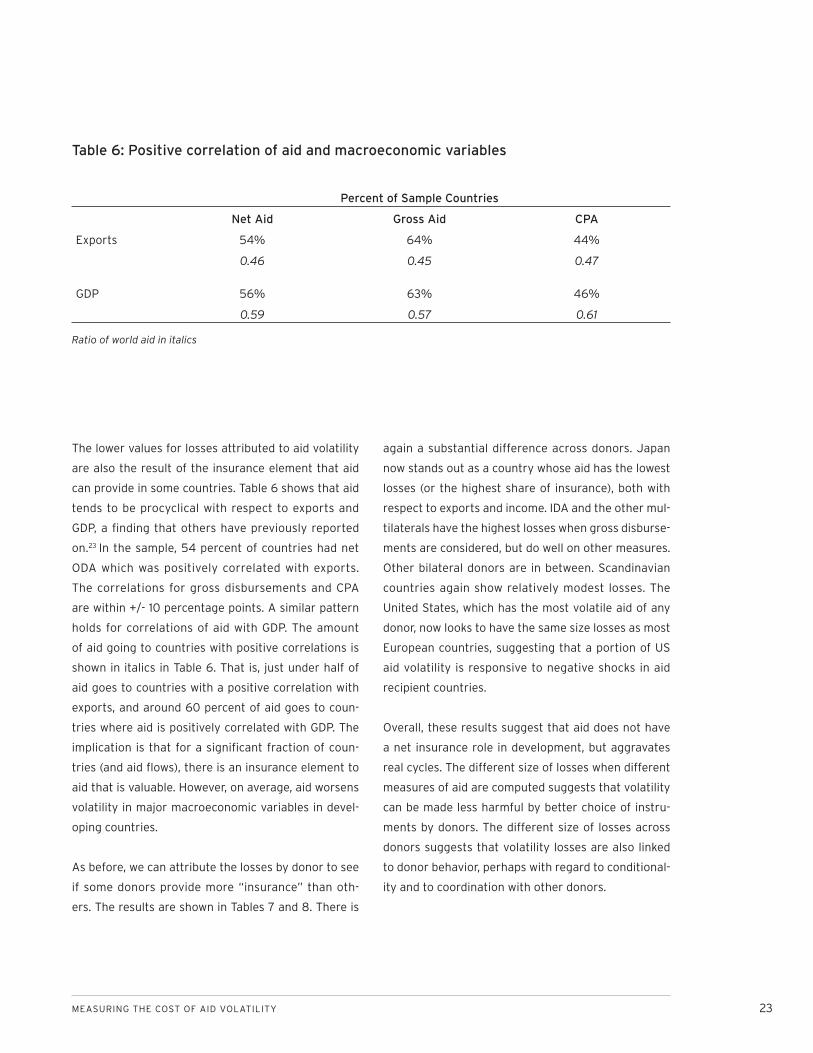
The lower values for losses attributed to aid volatility

are also the result of the insurance element that aid

can provide in some countries. Table 6 shows that aid

tends to be procyclical with respect to exports and

GDP, a fi nding that others have previously reported

on.23 In the sample, 54 percent of countries had net

ODA which was positively correlated with exports.

The correlations for gross disbursements and CPA

are within +/- 10 percentage points. A similar pattern

holds for correlations of aid with GDP. The amount

of aid going to countries with positive correlations is

shown in italics in Table 6. That is, just under half of

aid goes to countries with a positive correlation with

exports, and around 60 percent of aid goes to coun-

tries where aid is positively correlated with GDP. The

implication is that for a signifi cant fraction of coun-

tries (and aid fl ows), there is an insurance element to

aid that is valuable. However, on average, aid worsens

volatility in major macroeconomic variables in devel-

oping countries.

As before, we can attribute the losses by donor to see

if some donors provide more “insurance” than oth-

ers. The results are shown in Tables 7 and 8. There is

again a substantial difference across donors. Japan

now stands out as a country whose aid has the lowest

losses (or the highest share of insurance), both with

respect to exports and income. IDA and the other mul-

tilaterals have the highest losses when gross disburse-

ments are considered, but do well on other measures.

Other bilateral donors are in between. Scandinavian

countries again show relatively modest losses. The

United States, which has the most volatile aid of any

donor, now looks to have the same size losses as most

European countries, suggesting that a portion of US

aid volatility is responsive to negative shocks in aid

recipient countries.

Overall, these results suggest that aid does not have

a net insurance role in development, but aggravates

real cycles. The different size of losses when different

measures of aid are computed suggests that volatility

can be made less harmful by better choice of instru-

ments by donors. The different size of losses across

donors suggests that volatility losses are also linked

to donor behavior, perhaps with regard to conditional-

ity and to coordination with other donors.

Table 6: Positive correlation of aid and macroeconomic variables

Percent of Sample Countries

Net Aid Gross Aid CPA

Exports 54% 64% 44%

0.46 0.45 0.47

GDP 56% 63% 46%

0.59 0.57 0.61

Ratio of world aid in italics


Table 7: Exports portfolio, DWL from aid / aid, average 1970-2005

Donor nODA D CPA

France 0.120 0.094 0.070

USA 0.055 0.095 0.076

UK 0.053 0.046 0.016

EC 0.052 0.039 0.038

Germany 0.046 0.043 0.014

Norway 0.042 0.027 0.016

Netherlands 0.039 0.033 0.016

Sweden 0.037 0.029 0.013

IDA 0.026 0.121 0.022

Japan -0.015 0.002 -0.018

Other DAC 0.066 0.056 0.433

Other Bilateral 0.026 0.031 1.208


World 0.038 0.050 0.020

Table 8: GDP portfolio, DWL from aid / aid, average 1970-2006

Donor nODA D CPA

UK 0.093 0.089 0.053

France 0.063 0.058 0.013

Germany 0.032 0.035 -0.010

Netherlands 0.027 0.035 0.027

EC 0.018 0.020 0.015

USA 0.018 0.029 0.056

IDA 0.010 0.173 0.011

Sweden 0.009 0.015 -0.002

Norway 0.006 0.010 0.001

Japan -0.004 0.014 -0.013

Other DAC 0.035 0.040 -0.348

Other Bilateral 0.040 0.038 1.093


World 0.022 0.043 0.006


CONCLUDING REMARKS

We have presented evidence to show that aid vol-

atility results in substantial deadweight losses

for aid recipient countries. These losses could amount

to as much as 15 percent of total aid, or around $16 bil-

lion annually at current aid levels. We have also shown

that aid tends to aggravate major macroeconomic

variables, worsening real business cycles in develop-

ing countries. Reducing the harmful effects of aid

volatility should be a priority for donors.

In reaching this conclusion, we are consistent with

mainstream development thinking. The idea that

policy measures to reduce volatility should be a pri-

ority for development is now common. The most

evident example of this is the growing use of “fi scal

rules” for large commodity exporters. Countries such

as Chile and Nigeria have established off-shore funds

and budget rules to smooth government spending in

the face of large government revenue fl uctuations

coming from copper and oil price fl uctuations respec-

tively. These measures enjoy universal support among

development policy advisers.24 So it seems incongru-

ous that rules for smoothing aid, which is even more

volatile that exports in developing countries, are not

given more attention.

This paper provides a simple quantitative formula

for measuring the deadweight losses associated with

aid volatility. We recommend that offi cial aid donors

agree on a target for reducing these losses over the

next fi ve years. Unlike other estimates of losses from

aid volatility, the formula can be updated annually

and does not depend on complex country-by-country

models, on assumptions about key country param-

eters, or on cross-sectional regression results. Instead

it is based on parameters that are commonly used in

fi nancial markets.

The formula has one other advantage. It is decompos-

able into contributions from individual donors. We

would recommend that large donors, in particular, pay

close attention to the impact of their activities on ag-

gregate aid volatility. There are already agreements

and targets among donors as to the size of aid contri-

butions and limits on the degree to which aid should

be tied. In the same spirit, we recommend that there

should be a target for each donor on the losses asso-

ciated with volatility from its aid donations. With the

formula developed in this paper, the targets for each

donor would be transparent and easily monitorable.

If policymakers should choose to respond, there are

a number of technical proposals that could be imple-

mented to help limit volatility. Cohen et al. (2008) sug-

gests automatically linking repayment on soft credits

with an export shock, using a countercyclical loan

instrument, and implicitly targeting net foreign ex-

change at some level. Berg et al. (2007) proposes that

the IMF should permit countries to draw down foreign

exchange reserves when there are aid shortfalls and

that this option should be built into fi nancial program-

ming models. That would reduce the aggregate losses

from aid volatility. Others have argued that the size of

budget support should be adjusted to target net ODA,

by having one donor (perhaps IDA) act as a “donor of

last resort.”25 Countries may also make more use of

special accounts.26

Donors could also coordinate aid better to smooth

aggregate volatility. The current system of proliferat-

ing donors and projects with lumpy shifts in aid is too

clumsy to achieve smooth resource transfers. Donors

are unwilling to make individual long-term commit-

ments to aid recipient countries because of their

domestic budget procedures. But they could perhaps

do considerably better in indicating amounts they

would support as a collective over the medium term.


Already, some donors are moving towards multi-year

commitments to individual countries. That is a good

start. Finally, donors may want to consider institu-

tional arrangements that would make aid less volatile.

Scandinavian countries, that appear to have the low-

est volatility among bilateral donors, have parliamen-

tary approval of priority countries for aid allocations

and an explicit discussion on aid strategies. Such in-

stitutional lock-in can limit executive discretion in a

desirable way.


REFERENCES

Agénor, P., N. Bayraktar and K. El Ayanoui (2005).

“Roads out of Poverty? Assessing the Links

between Aid, Public Investment, Growth and

Poverty Reduction,” World Bank Policy Research

Working Paper, no. 3490.

Agénor, P. and J. Aizenman (2007). “Aid Volatility and

Poverty Traps,” NBER Working Paper, no. W13400.

Aghion, Philippe et al. (2005). “Volatility and Growth:

Credit Constraints and Productivity-Enhancing

Investment,” NBER Working Paper, no. 11349.

Barro, R.J. (2006). “Rare Disasters and Asset Markets

in the Twentieth Century,” Quarterly Journal of

Economics, 121(3): 823-866.

Berg, et al. (2007), The Macroeconomics of Scaling Up

Aid. Washington, DC: IMF.

Bulíř, A. and A. J. Hamann (2006). “Volatility of

Development Aid: From the Frying Pan into the

Fire?,” IMF Working Papers, 06/65.

Bulow, J. and K. Rogoff (1990). “Cleaning up Third-

World Debt Without Getting Taken to the

Cleaners,” Journal of Economic Perspectives,

4(1): 31-42.

Cassen, R. (1994). Does Aid Work. Oxford UP.

Cohen, D., H. Djoufelkit-Cottenet, P. Jacquet and

C. Valadier (2008). “Lending to the Poorest

Countr ies : A New Counter-cycl ica l Debt

Instrument,” OECD Development Centre Working

Paper, no. 269.

Department for International Development (2006).

Assessing the Volatility of International Aid Flows.

Reading, UK: Government of the United Kingdom/

Enterplan Ltd.

DESA (Department of Economic and Social Affairs)

(2005). World Economic and Social Survey. New

York: United Nations.

Eifert, B. and A. Gelb (2006). “Improving the Dynamics

of Aid: Toward More Predictable Budget Support,”

in Budget Support as More Effective Aid?

Recent Experiences and Emerging Lessons,

eds. S. Koeberle, Z. Stravreski, and J. Walliser.

Washington, DC: The World Bank.

Fatas, A. and I. Mihov (2008). “Fiscal Discipline,

Volatility and Growth,” in Fiscal Policy, Stabilization

and Growth, G. Perry, L. Serven and R. Suescun,

eds., Washington, DC: The World Bank.

Fielding, D. and G. Mavrotas (2005). “On the Volatility

of Foreign Aid: Further Evidence,” Paper pre-

pared for UNU-WIDER Project Meeting, Helsinki,

September 16-17.

Flyyholm, K. (2007). “Assessing Chile’s Reserve

Management,” IMF Survey Magazine Online.

Available: http://www.imf.org/external/pubs/ft/

survey/so/2007/car1126b.htm.

Geginat, C. and A. Kraay (2007). “Does IDA Engage in

Defensive Lending?” World Bank Policy Research

Working Paper, no. 4328.

Hnatkovska, V. and N. Loayza (2003). “Volatility and

Growth,” World Bank Policy Research Working

Paper, no. 3184.

IMF (2005). “The Macroeconomics of Managing

Increased Aid Inflows: Experiences of Low-

Income Countries and Policy Implications,” Policy

Development and Review Department.

(2007). “Staff Report for the 2007 Article IV

Consultation with Chile.” Available: http://www.

imf.org/external/pubs/ft/scr/2007/cr07333.pdf.


Kahneman, D., and A. Tversky, eds. (2001). Choice,

Values and Frames. New York: Cambridge UP.

Khamfula, Y., M. Mlachila and E.W. Chirwa (2006),

“Donor Herding and Domestic Debt Crisis,” IMF

Working Paper, no. 06/109.

Kharas, H. (2007). “Trends and Issues in Development

Aid,” Wolfensohn Center for Development,

Working Paper no. 1.

Levin, V. and D. Dollar (2005). “The Forgotten States:

Aid Volumes and Volatility in Diffi cult Partnership

Countries,” mimeo/unpublished manuscript for

the DAC Learning and Advisory Process.

Lucas, R. (2003). “Macroeconomic Priorities,”

American Economic Review, 93(1): 1-14.

Mart in , J. and G. Morgan ( 1988). “Financial

Planning Where the Firm’s Demand for Funds

is Nonstaionary and Stochastic,” Management

Science, 34(9): 1054-1066.

Newbery, D.M.G., and J.E. Stiglitz (1981). The Theory of

Commodity Price Stabiliation. Oxford: Clarendon Press.

Pallage, S. and M. Robe (2001). “Foreign Aid and

the Business Cyle,” Review of International

Economics, 9(4): 641-672.

Pallage, S., M. Robe, and C. Bérubé. (2006). “On the

Potential of Foreign Aid as Insurance,” IMF Staff

Papers, 53(3): 453-475.

Persson, T. and G. Tabell ini (2001). “Political

Institutions and Economic Policy Outcomes: What

Are the Stylized Facts?”, mimeo, IGIER.

Rabin, M. (2002). “A Perspective on Psychology

and Economics,” Working Paper no. E02-313,

University of California, Berkeley.

Ramey, G. and V. A. Ramey (1995). “Cross-country

Evidence on the Link Between Volatility and Growth,”

American Economic Review, 85(5): 1138-1151.

Rice, S. and S. Patrick (2008). Index of State Weakness

in the Developing World . Washington, DC:

Brookings.

Rietz, T.A. (1988). “The Equity Risk Premium: A

Solution,” Journal of Monetary Economics, 22:

117-131.

Schnabel, G. (2007). “Exchange Rate Volatility and

Growth in Small Open Economies at the EMU

Periphery,” European Central Bank Working

Paper, no. 773.

Shi, M. and J. Svensson (2001). “Political Budget

Cycles: Do they Differ Between Developed and

Developing Countries?,” mimeo.

Sharpe, W.F. (1966). “Mutual Fund Performance,”

Journal of Business, pp. 119-138.

(1994). “The Sharpe Ratio,” Journal of Portfolio

Management, 21(1): 49-58.

Ter-Minassian, T. (2007). “The Role of Fiscal Institutions

in Managing the Oil Revenue Boom,” IMF, Fiscal

Affairs Department. Available: http://www.imf.org/

external/np/pp/2007/eng/030507.pdf.

Tressel, T. and A. Prati (2006). “Aid Volatility and

Dutch Disease: Is There a Role for Macroeconomic

Policies?,” IMF Working Papers, 06/145.

Turnovsky, S. and P. Chattopadhyay (1998). “Volatility

and Growth in Developing Economies: Some

Numerical Results and Empirical Evidence,”

mimeo. Available: http://www.econ.washington.

edu/user/sturn/volatility_growth.pdf.


ENDNOTESSee Cassen, et al. (1994) for a complete summary.

Hnatkovska and Loayza (2003), Ramey and Ra-

mey (1995).

In this spirit, Newbery and Stiglitz (1981) show

foreign exchange reserve management and fi s-

cal rules can be better instruments for managing

commodity price risk than commodity stockpil-

ing.

Agenor et al. (2005) is an excellent example of

a computable general equilibrium model applied

to Ethiopia. Turnovsky and Chattophadhay (1998)

develops a stochastic general equilibrium growth

model.

I am grateful to Owen Barder from the UK’s De-

partment for International Development for his

insistence that without such a measure the pros-

pects for signifi cant change in the system are not

good.

We also looked at aid and government revenues

but found (to our surprise and disappointment)

that revenue data are not readily available with-

out loss of a signifi cant portion of the data set. It

also proved impossible to break down aid into its

on-budget and off-budget components.

See www.oecd.org/dac/stats/idsonline.

Cf. Bulow and Rogoff (1990), Geginat and Kraay

(2007).

Some analysts look at aid/capita or aid/GNP but

there is little reason to consider such transforma-

tions. We are interested in the total value of aid

and the discount associated with its volatility.

This fi nding was confi rmed through a cross-coun-

try regression analysis. The independent variables

are not signifi cant determinants of aid volatility.

The defi nition and measure of weak states is tak-

en from Rice and Patrick (2008). This fi nding sup-

ports Levin and Dollar (2005).

Barro (2006) fi nds 33 “disasters” for 20 OECD

countries in the twentieth century, that is in 2000

1.

2.

3.

4.

5.

6.

7.

8.

9.

10.

11.

12.

possible country-years.

Many countries witnessing aid shocks have had

internal or external confl icts. But this does not

necessarily justify high volatility. Donors could

anticipate vulnerable situations and limit the

degree of aid dependency for volatile countries.

There is also a recognition that donors might be

withdrawing aid too rapidly from post-confl ict

environments, as in East Timor, leading to cycles

of large aid infl ows, withdrawals and renewed

aid as a country cycles through confl ict periods.

S = E (r

m - r

f )

Var (rm - r

f ), following Sharpe (1994).

The losses for the CPA do not show the same pat-

tern, but some caution is in order as the data on

the breakdown of aid between its various compo-

nents is not thought to be complete or accurate in

early years. Thus, we believe the CPA to be poorly

measured before 1990.

Agenor and Aizenmann (2007) model this for-

mally in terms of an optimal contingency fund to

counteract aid volatility.

For example, Shi and Svensson (2001).

Kahneman and Tversky (2001); Rabin (2002).

IMF (2005) looked at 5 African countries and

found an average absorption rate of only 23 per-

cent for aid surges. That is, 77 percent of aid in-

creases between the late 1990s and early 2000s

was saved in reserves. However, much of the aid

was spent by government, resulting in an offset-

ting reduction in spending by the private sector.

Khamfula, Mlachila and Chirwa (2006), DESA

(2005).

Department for International Development

(2006), p.21.

We also attempted to look at a portfolio of total

revenues comprised of aid plus domestic rev-

enues. Unfortunately, domestic revenue data is

very incomplete. We would have had to drop more

than half the countries from the sample. The time

13.

14.

15.

16.

17.

18.

19.

20.

21.

22.


series data, required to produce robust volatility

calculations, also appears to be incomplete, with

changes in methodology in the IMF’s Government

Financial Statistics creating short series that can-

not be linked. For some countries, we fi nd that aid

is actually greater than reported total revenues in-

cluding aid! This is clearly impossible and is prob-

ably due to signifi cant underreporting of aid in

budget data. We therefore reluctantly abandoned

the extension of the calculations to revenue.

Pallage and Robe (2001).

Cf. Flyvholm (2007), IMF (2007), Ter-Minassian

(2007).

Eifert and Gelb (2006).

Special Accounts are revolving funds that reduce

the time for processing reimbursable expenses on

a project and help borrowers overcome cash fl ow

problems.

23.

24.

25.

26.

Selected photos courtesy of the World Bank: cover left to right: (#4) Ami Vitale, (#6) John Isaac

The views expressed in this working paper do not necessarily refl ect the offi cial position of Brookings, its board or the advisory council members.

© 2007 The Brookings Institution

ISSN: 1939-9383

Printed on recycled paper with soy-based inks.

1775 Massachusetts Avenue, NWWashington, DC 20036202-797-6000www.brookings.edu/wolfensohncenter

Measuring the Cost of Aid Volatility - Brookings · PDF filemeasuring the cost of aid...

Documents

Transcript of Measuring the Cost of Aid Volatility - Brookings · PDF filemeasuring the cost of aid...