Measuring Plant Lighting - Inda-Gro · Measuring Plant Lighting There are a number of ways to...

6 1 7 6 F e d e r a l B l v d . , S a n D i e g o , C A 9 2 1 1 4 - 1 4 0 1

T o l l F r e e : 8 7 7 . 4 5 2 . 2 2 4 4 L o c a l : 6 1 9 . 2 6 6 . 4 0 0 4 w w w . i n d a - g r o . c o m

Measuring Plant Lighting There are a number of ways to measure indoor plant lighting levels. As such, there remains considerable debate as to which method provides the gardener with the best information in determining if the light source is providing the ideal wavelengths and intensities to optimize plant response. While the debate swirls it ultimately will always come down to our plant’s response to those spectrums and intensities.

We recognize that the complexities of understanding and choosing which technology, or lamp, is best suited for gardening with indoor artificial lighting can be confusing. We publish our lamp’s output data in a format that you may not be familiar with, but we believe it offers the gardener a better opportunity to determine how much energy a lamp emits between 400-700 nm relative to generally accepted photosynthetic absorption regions.

As you can see by this Net Action Absorption Chart, what is believed to be the areas of greatest importance for a lamp’s energy to meet peak chlorophyll absorption points would be in the Vegetative Regions (Ultraviolet-Blue) and Flowering Regions (Red-Far Red). Less energy is required of the Carotenoid region (Green-Yellow) but as you can see there is still need for the lamp to emit within this region.

Grow lamp manufacturers produce Spectral Distribution Graphs for their lamps that graphically depict where the lamp will output wavelengths and in what intensities those wavelengths will emit. This works well in allowing the consumer to determine the lamps spectral output characteristics. The gardener can then decide if that particular lamp would work best for the type of plant being grown, specific growth cycles or if the spectrum is broad enough to take the plants from a vegetative thru a flowering state utilizing a single lamp.

In determining the proper lamp to purchase, the gardener will sometimes mistakenly rely on numerically driven data such as a comparison of lumen output, lumen/watt, kelvin, lux, and µmole ratings to name a few. For plant lighting comparisons, each of these values will at best give incomplete information and at its worse, will provide you with information that is mostly irrelevant to what your plants actually require from the lamp.

A more informed approach relies on a review of the manufacturer’s spectral distribution graph. Once installed, the gardener will still want to measure light intensity to have complete lamp performance data. These types of field intensity measurements are usually made with a modestly priced PAR meter which has been calibrated to the sun and not the artificial light source being measured. Which leads us to why we do not publish our lamp output data based on:

• Lumens, Lumens/Watt, Lux or Foot Candles -These are all measurement terms that by definition use light meters which reference intensities adjusted to the human photopic luminosity function. They have little bearing on how a plant will respond to the intensities being emitted in visual regions.

• Kelvin – This is another human visual standard that references how the light appears overall to the eye with 555 nm being peak visual sensitivity and 510/610nm being ½ peak visual sensitivity. As higher Kelvin value imply, more blue to red ratio and lower Kelvin values would indicate a greater red to blue ratio. Basing your grow lamp decision based on how much visual red or blue a lamp emits is not a good means of determining if that lamp is meeting the actual absorbance regions.

• µMole – This value is attained by using a PAR meter which is a better meter for reading plant intensity values in that it is not correcting for human photopic luminosity function, like a meter reading lumens, lux or footcandles will do, it still has some of its own issues. The problem with relying too heavily on a µMole value is that it is based on the total light intensity in the 400-700 nm range and



does not account for the spectral points within that range. This issue is further complicated by the fact that PAR meters actually measure light intensity (not actual photon counts), it must assume a spectral distribution to actually assign a uMol/M2-S value. This assumed spectral distribution for a PAR meter will normally be natural sunlight, but for artificial light, with a different spectral distribution, errors will occur. For example, shorter wavelength photons have more energy than longer wavelength photons; a 420 nm photon has 1.5 times the energy of a 630 nm photon. If a particular light source was very heavy in the violet and blue region the PAR meter, based on its calibration, would likely yield a higher uMol/M2-S based on its sunlight calibration assuming that some of that additional light energy from the blue must be red.

Not having a weighted µMole value is also problematic when dealing with narrow spectrum technologies such as LED panels. Manufacturers will often advertise high intensities of 2000 µMoles @ 24” from the source. While that reading might very well be in a peak absorption region, it could easily be a reading in a green-yellow region, or of such narrow bandwidth, that its output is of little value to the plants overall or regional net action absorption requirements. It is for these reasons a complete determination of the lamps output should include reference to the manufacturers spectral distribution graph as well as the amount of energy being expended in the three PAR absorbance regions.

As manufacturers, we need to publish artificial lighting data in a metric that will enable the gardener to have a numerical value which describes the lamps value in both plant spectrums and intensities. A single number, such as lamp lumen output, does not provide the gardener with meaningful data. We believe that by providing the gardener values which take into account lamp energy efficiencies, within photosynthetically active absorbance regions, it allows them to make a more informed decision when purchasing lamps for their garden.

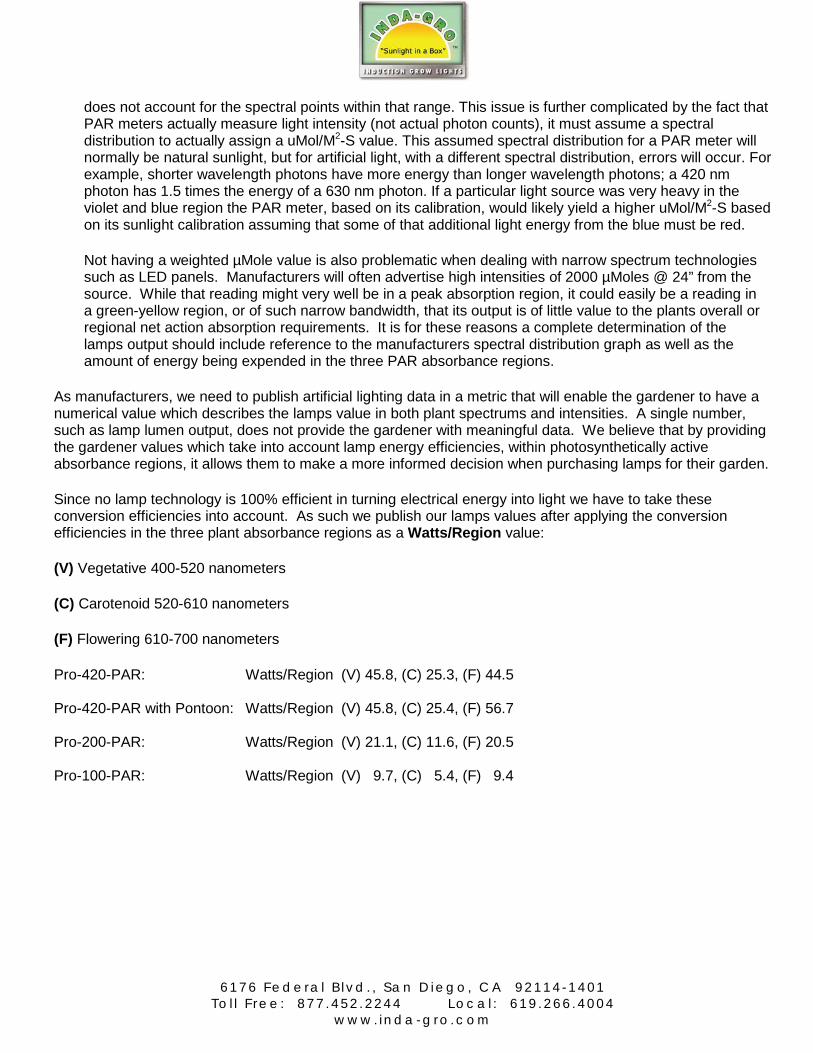
Since no lamp technology is 100% efficient in turning electrical energy into light we have to take these conversion efficiencies into account. As such we publish our lamps values after applying the conversion efficiencies in the three plant absorbance regions as a Watts/Region value:

(V) Vegetative 400-520 nanometers

(C) Carotenoid 520-610 nanometers

(F) Flowering 610-700 nanometers

Pro-420-PAR: Watts/Region (V) 45.8, (C) 25.3, (F) 44.5 Pro-420-PAR with Pontoon: Watts/Region (V) 45.8, (C) 25.4, (F) 56.7 Pro-200-PAR: Watts/Region (V) 21.1, (C) 11.6, (F) 20.5 Pro-100-PAR: Watts/Region (V) 9.7, (C) 5.4, (F) 9.4



Questions and Answers:

1. Does knowing the V-C-F values of the lamps output eliminate the need for the lamp manufacturers Spectral Distribution Graphs?

The V-C-F values represent the total watts being consumed within these 3 regions. It does not replace a Spectral Distribution Graph which enables the grower to determine precise spectrums within these regions where the majority of the energy is being consumed.

2. Does knowing the V-C-F value eliminate the need for field measurements of lighting intensities?

The grower would be advised to continue using a quantum PAR meter for initial lamp intensity output at set determined distances from the lamp to meet proper crop Photosynthetic Photon Flux Densities (PPFD) and enable the grower to monitor intensity depreciation at the beginning of each crop cycle.

3. Can you explain how V-C-F values are achieved?

This process relies on knowing the spectral distribution of the lamp and how much energy it consumes at each individual wavelength and adding that together to show the watts consumed within that region. The manufacturer must have the equipment to take spectral distribution measurements from within that limited V-C-F bandwidth and then publish it in a watts/region format.

4. If I only have a standard light meter that measures Lux, Lumens and Foot Candles can I use that meter to test intensities between my crop cycles?

While we still recommend a quantum meter a typical photographic type of meter (photometer) will measure intensities loses in the Visible/Carotenoid (C) region of the 520-610 regions spectrum. The relative intensity losses within the (V) and (F) regions would be fairly proportional to the losses in the (C) region.

5. I’ve not seen other manufactures adopt this approach to publishing their lamps output. Are there other methods that would give the grower enough information to compare lamp outputs?

Part of the problem is that lighting manufactures do not have a generally accepted industry standard plant absorbance sensitivity curve that manufacturers can point their lamps output data relative to that curve. The problem has been identifying a meaningful curve that is broad enough to cover a majority of plant species net absorption regions. Many manufacturers will refer to the German DIN Standard 5031-10 but this has not been accepted as, nor should it be, a hard and fast standard for all plant species.



6. If two manufacturers have posted identical V-C-F values can a gardener presume the results will be the

same?

The short answer is no. But this answer also depends on the previous answer where specific plant sensitivity curves would ultimately tell which lamp is emitting within the peak absorption ranges that are ideal for that particular plants photosynthetic processes. Watts/Region is a way to determine how much energy the lamp is emitting within that region. Since each region is broad enough that specific wavelengths within those regions may be drawing most of the energy plant response can vary with identical V-C-F values as a result of spectral differences within the regions. It is entirely possible that when comparing two lamps with identical V-C-F values that one lamp will outperform the other. Think of it this way; you can go into two separate restaurants and order lasagna. Both chefs will have the same or similar ingredients to get to the final dish. Both dishes have the same calories but one dish may be substantially better tasting and better for you. Plants will react the same way when ‘fed’ light where wavelengths within the watts/region are different between the two lamps.

7. Do reflector or fixture designs enter into the Watts/Region values? They do not. As in the previous two answers when comparing identical or even higher values, other considerations would be actual spectral distribution within the three regions. Beyond that other factors to consider would be:

• How much heat a lamp/ballast combination contribute to the grow room • Light being emitted outside of 400-700nm • Intensities at the canopy (PPFD) • Spectral distribution within each region • Fixture design as thermal management • Reflector design and quality • Lamp size and shape • Consistency of spectral mix from the lamp(s) to the canopy

8. If I know the lamps V-C-F values what should be considered when interpreting a lamps output based on

its spectral distribution?

When you have the V-C-F value you are interpreting the amount of energy under the height and width of the data points shown within these graphs. For example a graph showing a high peak thin sliver intensity at a specific wavelength may not contribute as much to a plants development as a lower peak wider spectrum. To illustrate this point we would refer you to the DIN 5031-10 where you can see the radiant power differences between HID and LED relative to the plants sensitivity curve. Ideally one should consider lamps spectral output characteristics in terms of its ability to show: • Some baseline broad spectrum coverage between 400-700nm • Lamp to Plant efficiencies: Higher intensities in the known high PAR absorption regions • Broad enough spectrums within the plants PAR absorption regions Armed with this information one should also consider the importance of lamp lifespan, i.e. replacement costs and spectral stability as the lamp ages to maintain repeatable crop production.



V-C-F Plant Light Specification Technique

Definitions of each of the 5 specification techniques

1. Radiant PAR Wattage: The actual light power produced in the PAR region. 2. PPF: Photosynthetic Photon Flux expressed in uMol/S is the actual number of photons produced per

second in the PAR region. 3. Photopic Lumen: Nearly useless for plant lighting, but it is so commonly used we felt it important just

to show how misleading it can be when compared to the other valuations. Lumens are light power values for human vision expressed in units which have been corrected to the CIE accepted conversions per the photopic luminosity function for the specified wavelength bandwidths. While Lumens are commonly specified for plant lights, this specification should never be used in making a decision on plant lighting as it is a strict reference to how humans see light.

4. Yield PPF: The light power values within the PAR region shown in uMol/S which have been adjusted to the DIN standard 5031-10 sensitivity curve.

5. Yield PAR Watts to DIN 5031-10: These values are actual radiant watts adjusted to the DIN Standard 5031-10 absorption sensitivity. While the Radiant PAR Watt is an indicator of actual light power produced in the PAR region, the Yield PAR Watt is an indicator of what the plant should be able to actually absorb under ideal conditions.

Definitions of the various parameters used for the 5 specification techniques

o Absolute Values: These are the actual values for the lamp wattage rating shown for each of the 5 defined categories.

o 400-520 (V): These are the absolute values for the Vegetative (V) region (400 to 520 nm) only. o 520-610 (C): These are the absolute values for the Carotenoid (C) region (520 to 610 nm) only. o 610-700 (F): These are the absolute values for the Flowering (F) region (610 to 700 nm) only. o Total 400-700: These are the absolute values for the Total PAR region (400 to 700 nm) only. o Efficiencies: These are the Total values factored on a per Watt consumed basis. This value generally

represents an overall efficiency rating for each lamp technology for each of the 5 types of measurements and can be compared one to one since they have all been adjusted for consumed wattage.

o Percentages: These are the percentage breakout of each of the 3 regions V, C, and F to the Total. The values can be used to make one to one comparisons of the different lamp technologies for each of the 5 measurement techniques.

Notes:

1. Both CMH and Plasma have a degree of intensity that is emitted outside of the defined PAR region of 400 to 700 nm. This does result in lower values in the PAR region. This is just an explanation should there be any curiosity of these lower values, but they are valid.

2. Since LED lamp designs can vary widely we chose a lamp that represented the fairly typical of the Blue/Red combinations seen.



Technical Comparisons

Radiant Wattage Consumed Watts

Absolute Values Total 400-700

Radiant Efficiency

Percentages

400-520 520-610 610-700 400-520 520-610 610-700 HPS Digital 1000 watts 1100 18.6 173.8 110.5 302.9 0.275 6 57 36

HPS Digital 600 watts 660 12.3 114.7 72.9 199.9 0.303 6 57 36

M/H Digital 4000K 1000 watts 1100 76.5 155.0 35.5 267.0 0.243 29 58 13


CMH Magnetic 4000K 400 watts 480 29.0 34.4 28.1 91.5 0.191 32 38 31

PLASMA 300 watts 300 26.5 22.6 16.6 65.7 0.219 40 34 25

T5-HO 6500K 54 watts 58 5.6 5.9 1.7 13.2 0.228 43 44 13

T5-HO 2800K 54 watts 58 1.8 6.3 4.1 12.2 0.210 15 52 33

LED - LG650 650 watts 650 69.5 19.1 149.3 238.0 0.366 29 8 63

EFDL IG-Pro-420 420 watts 425 45.8 25.3 44.5 115.6 0.272 40 22 38

EFDL IG-420/Pontoon 460 watts 460 45.8 25.4 56.7 127.9 0.278 36 20 44

PPF (uMol/S) Consumed Watts


uMol/S per Watt

Percentages

400-520 520-610 610-700 400-520 520-610 610-700 HPS Digital 1000 watts 1100 72 848 587 1506.3 1.37 5 56 39

HPS Digital 600 watts 660 47 560 387 994.0 1.51 5 56 39

M/H Digital 4000K 1000 watts 1100 302 738 192 1230.9 1.12 24 60 16


CMH Magnetic 4000K 400 watts 480 112 163 152 428 0.89 26 38 36

PLASMA 300 watts 300 103 107 90 300.0 1.00 34 36 30

T5-HO 6500K 54 watts 58 21 28 9 58.0 1.00 37 47 16

T5-HO 2800K 54 watts 58 7 30 21 58.0 1.00 12 52 37

LED-LG650 650 watts 650 258 91 821 1170.4 1.80 22 8 70

EFDL IG Pro-420 420 watts 425 174 122 237 533.0 1.25 33 23 44

EFDL IG-420/Pontoon 460 watts 460 174 122 303 599.0 1.30 29 20 51

Photopic Lumen Consumed Watts


Lumen per Watt

Percentages





CMH Magnetic 4000K 400 watts 480 3187 19568 3235 25990.0 54.1 12 75 12

PLASMA 300 watts 300 3026 13079 1917 18022.0 60.1 17 73 11

T5-HO 6500K 54 watts 58 472 3520 378 4370.0 75.0 11 81 9

T5-HO 2800K HO 54 watts 58 131 3620 892 4644.0 80.0 3 78 19

LED-LG650 650 watts 650 3004 10889 9245 23137.4 35.6 13 47 40

EFDL IG-Pro-420 420 watts 425 3518 13751 7999 25268.0 59.0 14 54 32




Yield PPF (uMol/S) Based on DIN 5031-10 Sensitivity Curve

Consumed Watts


YPPF per Watt

Percentages





CMH Magnetic 4000K 400 watt 480 90 80 112 282.0 0.587 32 28 40

PLASMA 300 watts 300 82 52 66 200.0 0.670 41 26 33

T5-HO 6500K 54 watts 58 18 13 6 37.0 0.630 49 34 17

T5-HO 2800K 54 watts 58 5 15 15 35.0 0.600 15 42 43

LED-LG650 650 watts 650 237 46 652 935.0 1.440 25 5 70

EFDL IG-Pro-420 420 watts 425 143 63 171 377.0 0.890 38 17 45


Yield PAR Watts Based on DIN 5031-10 Sensitivity Curve

Consumed Watts


PAR Watt Efficiency

Percentages

400-520 520-610 610-700 400-520 520-610 610-700 HPS Digital 1000 watts 1100 15.5 93.9 79.7 189.0 0.172 8 50 42

HPS Digital 600 watts 660 10.2 62.0 52.6 125.0 0.190 8 50 42



CMH Magnetic 4000K 400 watt 440 23.4 16.8 20.6 61 0.127 39 28 34

PLASMA 300 watts 300 21.3 10.9 12.2 44.5 0.148 48 25 28

T5-HO 6500K 54 watts 58 4.7 2.7 1.2 8.6 0.150 55 31 14

T5-HO 2800K 54 watts 58 1.4 3.0 2.9 7.3 0.130 19 42 39

LED-LG650 650 watts 650 64.1 9.5 118.6 192.1 0.296 33 5 62

EFDL IG-Pro-420 420 watts 425 38.1 12.9 32.3 83.0 0.200 46 15 39

EFDL IG-420/Pontoon 460 watts 460 38.1 13.0 42.1 93.0 0.200 41 14 45 Technical Comparisons Summary Conclusions: In developing this document we used manufacturer data that was available at the time of this publication from a variety of manufacturer’s websites. Nothing in this document is meant to construe that we are suggesting that any one technology is better than the other. Our interest in developing this document was to simply present another way of viewing how artificial plant lighting can be presented in a way that does not confuse the gardener with information and values that may be mostly irrelevant when it comes to selecting the best lamp for their needs. We are not saying that the reporting methods we’ve suggested here cannot be improved upon. For example V-C-F is not meant to imply that a lamp which emits predominantly in the C-F regions would be the most beneficial to a flowering plant that might develop even better with a higher percentage of V. We believe that as manufacturers it is our responsibility to be environmentally conscious while looking to continuously expand upon all available technologies which serve to enhance crop production, increase quality and bring a greater overall value to the indoor garden.



Equations used for the Calculation of the V-C-F values

The ideal method of achieving these values would be to integrate the various equations across the spectral region that is generally considered the PAR region, 400 to 700 nm. Since these lamps spectral distribution outputs do not follow any workable mathematical functions, the best method to approximate the Integral is with a Summation equation across the PAR region. The more points used the better the accuracy of the summation function. Since 400 to 700 nm represents a nice spread of 300 points at 1 nm increments this was the obvious choice of increment and is enough points to assure some degree of good accuracy. Essentially using the Summation process all the math is performed on each 1 nm sliver and then the results of each sliver are added together for the final result. The subscript HPS is used to indicate those functions that are specific to a unique light source. Equations 1 through 5 below are the actual equations that our V-C-F values are based.

1.𝑅𝑎𝑑𝑖𝑎𝑛𝑡 𝑊𝑎𝑡𝑡𝑠𝐻𝑃𝑆 = � 𝑅𝑊𝐻𝑃𝑆

700

𝜆=400(𝜆) ≈ � 𝑅𝑊𝐻𝑃𝑆

700

𝜆=400(𝜆)

2. 𝑃𝑃𝐹𝐻𝑃𝑆 = � 𝑅𝑊𝐻𝑃𝑆

700

𝜆=400(𝜆) × 𝑀𝑃𝑊(𝜆) ≈ � 𝑅𝑊𝐻𝑃𝑆

700

𝜆=400(𝜆) × 𝑀𝑃𝑊(𝜆)

3. 𝐿𝑢𝑚𝑒𝑛𝐻𝑃𝑆 = � 𝑅𝑊𝐻𝑃𝑆

700

𝜆=400(𝜆) × 𝑃𝐿𝐹(𝜆) × 683 𝐿𝑢𝑚𝑒𝑛/𝑊𝑎𝑡𝑡

≈ � 𝑅𝑊𝐻𝑃𝑆

700

𝜆=400(𝜆) × 𝑃𝐿𝐹(𝜆) × 683 𝐿𝑢𝑚𝑒𝑛/𝑊𝑎𝑡𝑡

4. 𝑌𝑖𝑒𝑙𝑑 𝑃𝑃𝐹𝐻𝑃𝑆 = � 𝑃𝑃𝐹𝐻𝑃𝑆700

𝜆=400(𝜆) × 𝐷𝐴𝑆(𝜆) ≈ � 𝑃𝑃𝐹𝐻𝑃𝑆

700

𝜆=400(𝜆) × 𝐷𝐴𝑆(𝜆)

5. 𝑌𝑖𝑒𝑙𝑑 𝑃𝐴𝑅 𝑊𝑎𝑡𝑡𝐻𝑃𝑆 = � 𝑅𝑊𝐻𝑃𝑆

700

𝜆=400(𝜆) × 𝐷𝐴𝑆(𝜆) ≈ � 𝑅𝑊𝐻𝑃𝑆

700

𝜆=400(𝜆) × 𝐷𝐴𝑆(𝜆)



The last set of equations shows the 3 individual V-C-F regions as integrals and summations for the total 400 to 700 nm range.

� 𝑓(𝑦)700

𝜆=400

= � 𝑓(𝑦)520

𝜆=400

+ � 𝑓(𝑦)610

𝜆=520

+ � 𝑓(𝑦)700

𝜆=610

≈

� 𝑓(𝑦)700

𝜆=400

= � 𝑓(𝑦)520

𝜆=400

+ � 𝑓(𝑦)610

𝜆=521

+ � 𝑓(𝑦)700

𝜆=611

Definitions of Terms:

RW(λ) is the Radiant Watt function as a function of λ (Wavelength) for the light source.

PPF(λ) is the Photosynthetic Photon Flux function as a function of λ for the light source.

MPW(λ) is the photon uMol/S per Watt function as a function of λ.

PLF(λ) is the Photopic Luminosity Function as a function of λ.

DAS(λ) is the DIN 5031-10 Absorption Sensitivity function as a function of λ.

The MPW(λ) function is the conversion of light intensity in Watts to the quantity of photons in µMol/S as a function of wavelength (λ). The derivation of the equations is shown in our analysis “The Planck Relation”. This is nothing new, just a conversion of the Planck Relation equation to the terms we are more used to working with for lighting:

Wavelength in nm

Photons in µMol/S

Light Intensity in radiant watts



Converting Photon µMol/S count and intensity in Watts: The Planck Relation

E = hc/λ

E = Energy per Photon(λ)

h = 6.62606957 x 10-34 J-S (Planck’s Constant)

c = 2.99792458 x 108 M/S (Speed of Light)

λ = photon wavelength

We ultimately want to derive an equation that will relate light intensity Wattage to photon flux quantity in µMo/S as a function of wavelength λ.

PhotonµMol Power(λnm) Watts = hc x Mol x 10-6/λnm x 10-9 M-S

Where:

Mol = 6.0221413 x 1023

X 10-6 Converts photon quantity in Mol to µMol

X 10-9 Converts wavelength in M to nM

For equations going forward: Photon flux quantities are expressed in µMol/S and λ in nm.

PhotonµMol Power(λ) Watts = 6.62606957 X 10-34 J-S x 2.99792458 X 108 M/S x 6.0221413 X 1023 x 10-6/λnm X 10-9 M-S

= 119.626566/λnm J/S, J/S = Joules/S = Watts, Power = 119.626566 W-nm / λnm nm

Conversion Formulas: Enter wavelength in nm, Power in Watts, and PPF in µMol/S

PhotonµMol Power(λ) (Watts) = 119.626566/λnm X µMol/S

PhotonµMol(λ) Flux Quantity (µMol/S) = .00835935 X λnm X Watts



Measuring Light: The important differences between PPF and PPFD

There exists some industry inconsistencies between how PPF and PPFD is used when describing their lamps output. For those basing their decision on which lamp is best suited their garden it’s important to know what these different terms mean.

PPFD (Photosynthetic Photon Flux Density) µMol/M2S is certainly well defined, accepted and consistently used. However, PPF is used inconsistently by nearly every source referencing it. We have seen a quantum sensor manufacturer indicate that the terms PAR, PPF, and PPFD are all the same having units of µMol/M2S. We have also seen many refer to PPF in various ways having units of µMol/M2S. We have seen industry leading light manufacturers refer to PPF as the total radiant light output in the PAR region of a lamp in units of µMol/S. So the question is: If PPFD is well defined and uniformly accepted, why then are so many within the industry using PPF to have the same meaning?

The likely answer is that there is no good solid standard for the industry to work within. So taking a look at area lighting and their value definitions the best conclusion we can draw is that the units for PPF should be µMol/S. We think the reason for this confusion results from a disconnection between the lamp and sensor manufacturers, particularly since lamp specifications should be based on PPF and field measurements based on PPFD. Another issue contributing to the confusion is that so many manufacturers, both lighting and measurement, do not consistently show the complete proper engineering units in their marketing, operating, and specification documents.

PPF as µMol/S is the value that a grow lamp should specify for its total light output (Radiant Watts would also be appropriate), this would be similar to using Lumens for a regular area light. PPFD is the primary measurement taken by a Quantum PAR meter and is expressed as a density over a unit of area, this would be similar to using Lux or Foot-Candles on a regular light meter. We do believe these to be the proper definitions as originally intended, but have been unable to find any industry standard or document to substantiate that.

For your consideration:

PPF (Photosynthetic Photon Flux) issued by (or should be) manufactures as the lamps total emitted number of photons per second in the PAR region. Units of measure: µMol/S

PPFD (Photosynthetic Photon Flux Density) represents a field measurement and is defined as, the number of photons in the PAR region emitted per M2 per Second. Units of measure: µMol/M2S

In standard commercial/industrial lighting terminology the use of the term “flux” generally applies to the light energy on a per time basis which in grow lamps would be the lamps PPF value. By definition, Energy per time or energy transfer rate is defined as Power. In lighting terms, light power is generally defined in terms of Radiant Flux or Luminous Flux.

The point of this discussion is that the term “flux” used in the absence of density applies to energy or power emitted, but not over a specific area. The term “Density” generally applies to the energy or power per a volume of space, in the case of lighting, it generally applies to an area rather than a volume, since light striking a surface area is more applicable than light within a volume.

Lamp manufacturers should rate the lamps overall output in PPF (µMol/S) or PAR radiant Watts rather than Lumens which are strictly for human vision. Ideally in the future we may have a generally accepted PAR sensitivity standard that can be applied to give results as Yield PPF or Yield Radiant Watts which would be a more equivalent measurement to Lumens, but would be plant specific.



If a lighting manufacturer, not a lamp manufacturer, were to use PPFD as a specification for a particular fixture/lamp combination they would need to include all of the following information for the user to properly interpret the information being given:

1. Provide the height from which the measurement was taken. 2. Provide multiple locations across the illuminated footprint at meaningful points allowing for

interpretation of consistency of intensity and footprint limitations. 3. Provide multiple sets of PPFD measurements at different heights.

To publish in a PPFD value various considerations with this approach would be:

1. Measurements must be taken with reflectors in place to achieve accurate results. 2. For HID lamps since the lamps are sold separate from the reflectors there can be many different

combinations of lamps and reflectors. Any measurements taken need to be specific to a particular lamp/reflector combination.

3. At the close height that grow lamps are used their light distribution patterns will not change in a regular expected manner. The use of a reflector in the design requires that a certain minimum measurement distance is used for values to stabilize and act with an expected regularity for varying heights. This height in many cases will be greater than the typical height used for an indoor grow, but would likely be good for a greenhouse supplemental application. Basically we are referring to relationship of Light Intensity as a function of 1/d2, where d is the measurement distance from the light source. Until this certain height is achieved, you will not see measured values following this rule at all.

4. As for LED panels, these measurements will not stabilize until a height is reached for which the beam patterns of the LEDS have interlaced enough to be somewhat homogenous, both with respect to intensity and mixture of different LED wavelengths.

5. Interpreting the results of overlapping light from adjacent lamps in multiple lamp systems can be a difficult task, but would be necessary to determine the true quantity of light intensity at any particular point.

6. It will likely still take some field experimentation with proper measurement equipment and different configurations of the lamps to come to the optimal lamp placement, particularly in a multiple lamp system.

Summary Conclusions: PPF and PPFD certainly have their place when discussing grow lamp output values and how those values may then be measured in the field. However, there does exist inconsistencies on how lamp and sensor manufacturers use these terms and for the average gardener who may lack advanced degrees in Physics and Engineering, these are not going to be terms they can easily come to grips anyway. As such we felt introducing an alternative method, which was easier to comprehend, would be in order.

Understanding Spectral Distribution Graphs

Spectral Distribution Graphs (SDG) represents a graphic depiction of the light intensity (power) for the various wavelengths the lamp emits in a plotted format. Buyers without a formal understanding of this information will often mischaracterize the information assuming both positive and negatives that are not actually representative the SDG. We are going to introduce an example SDG and describe how to interpret it.



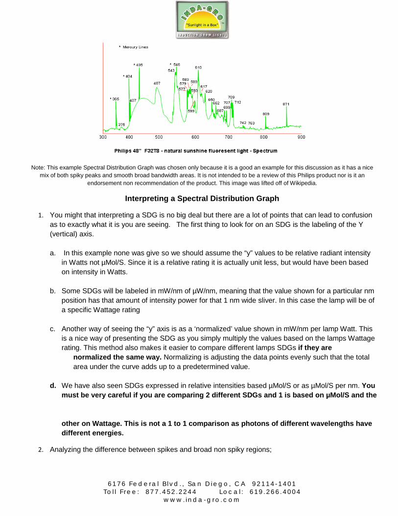
Note: This example Spectral Distribution Graph was chosen only because it is a good an example for this discussion as it has a nice

mix of both spiky peaks and smooth broad bandwidth areas. It is not intended to be a review of this Philips product nor is it an endorsement non recommendation of the product. This image was lifted off of Wikipedia.

Interpreting a Spectral Distribution Graph

1. You might that interpreting a SDG is no big deal but there are a lot of points that can lead to confusion as to exactly what it is you are seeing. The first thing to look for on an SDG is the labeling of the Y (vertical) axis.

a. In this example none was give so we should assume the “y” values to be relative radiant intensity

in Watts not µMol/S. Since it is a relative rating it is actually unit less, but would have been based on intensity in Watts.

b. Some SDGs will be labeled in mW/nm of µW/nm, meaning that the value shown for a particular nm

position has that amount of intensity power for that 1 nm wide sliver. In this case the lamp will be of a specific Wattage rating

c. Another way of seeing the “y” axis is as a ‘normalized’ value shown in mW/nm per lamp Watt. This

is a nice way of presenting the SDG as you simply multiply the values based on the lamps Wattage rating. This method also makes it easier to compare different lamps SDGs if they are

normalized the same way. Normalizing is adjusting the data points evenly such that the total area under the curve adds up to a predetermined value. d. We have also seen SDGs expressed in relative intensities based µMol/S or as µMol/S per nm. You

must be very careful if you are comparing 2 different SDGs and 1 is based on µMol/S and the other on Wattage. This is not a 1 to 1 comparison as photons of different wavelengths have different energies.

2. Analyzing the difference between spikes and broad non spiky regions;



a. First, for a fluorescent based lamp you will always have visible Hg (Mercury) spikes at 365, 405,

436, 546 and 580 nm. These are unavoidable if the lamp is Hg based. There can be some variation in the relative heights of the spikes which will be discussed later.

b. The main difficulty with SDG analysis is interpreting the spikes. The user has a tendency to see

these tall spikes and associate a high percentage of the output intensity to be at these values.

c. The proper way to determine the net intensity in a particular region is to take the total area

under the curve in that region. This is where SDGs shown in mWatts/nm are very straightforward: You can view each of the point heights of the curve nm by nm and simply sum each value to get the total value in the region. The sum of all of these silvers will nicely approximate the area under the curve.

d. Let’s take a look at our example SDG, at 546 nm we have our highest peak, this is a result of

the 546 nm Hg spike coupled with the 543 spike of the standard green component of a tri-phosphor blended lamp. While there may appear to be a lot of intensity at this point, it may not be as much as we think. Remember it is the area under the curve that sums to the total intensity for a particular region of the SDG. If I were to define the general region of this green spike to be about 540 to 575 nm, you can easily see that the regions to both the left and right have a greater area under the curve and therefore the net quantity of green light may not actually be that excessive.

3. Another item to look at on an SDG are the void areas or regions where there is no light intensity. On this example there are no serious void areas shown. This is actually fairly unusual for this type of phosphor blend and may be a result of some measurement equipment noise. Numerous and large void areas tend to be more of an issue with lamps that have very high or low Kelvin temperatures as they tend to lean heavily toward the blue or red regions. Looking at the SDG in this example we see no significant voids, this would be an indicator of a good broad spectrum lamp with a very high CRI. I would estimate a Kelvin temperature of about 5000 to 5500K and a CRI of 85 to 90. The actual specifications from Philips were a color temperature of 5000K and a CRI of 82. Our over estimation of the CRI may be a result of being fooled by the lack of void areas that may have resulted from measurement equipment noise.

4. A quick estimate of this SDG to our recently defined V-C-F measurement technique resulted in a V of 43.6%, C of 29.4% and F of 27.0%. Just looking at the VCF values would rate this as a fairly broad spectrum lamp with a high CRI. While it was made to be a visual lamp it likely would do a reasonable job as a grow lamp, no problem vegetative, but it would likely need some help for fruiting and flowering.

5. Also worth noting on this SDG is the presence of significant energy both below 400 nm and above 700 nm. While this light energy is still useful to a plant most all PAR or quantum meters will not measure it, but as earlier stated this may be measurement equipment noise.



Contributing elements to the distribution of this SDG

The following are the likely phosphors used in this particular lamp along with as many of the peaks that we could identify and the likely source of the peak.

1. Hg Mercury spikes: 365, 405, 436, 546, and 579 nm 2. BaMg2Al16O27:Eu2+ (most likely) (aka BAM): 452 nm peak with ½ height bandwidth of 51 nm,

accounts for most of the contribution 400 to 510 nm. 3. CeMgAl11O19:Tb3+ (most likely) (Green tri-phosphor component): Main peak at 544 nm, minor

peaks at 488, 577, 579, 584, 617, 621 nm 4. Y2O3:Eu3+ (Red tri-phosphor component): Main peak at 611 nm, minor peaks at 589, 593, 600, 650,

663, 688, 694, 707, 709, and 713 nm 5. Argon: 760, and 809 nm

Note: Constant energy levels shown below 400 nm and above 720 nm may be a result of measuring equipment noise.

Other factors that affect light output and the SDG of a lamp

1. Quantum efficiency of each phosphor: Mercury (Hg) has its primary emission at 253.7 nm (about 84.5% of the emitted energy) and a secondary emission at 185 nm (about 7% of the emitted energy), the balance are those earlier mentioned that are in the visible region to begin with (about 8.5% of the emitted energy). The 253.7 and 185 nm photons are typically absorbed and excite the phosphor molecule to emit its signature emission. But not all of the photons emitted by the mercury result in a phosphor generated emission. The Quantum Efficiency is defined as quantity of photons that achieve phosphor excitation resulting in a photon emission divided by the total number of 185 nm and 253.7 nm photons emitted. This value varies greatly from phosphor to phosphor.

2. Planckian Efficiency of the phosphor: We have defined this as the loss of quantum photon energy

resulting from the conversion of the Hg emitted photons to the lower energy, longer wavelength photons emitted by the phosphor. Per the Planck Relation Equation, we have E=hc/λ. E is energy, h Planck’s constant, c the speed of light, and λ the photon wavelength. A quick and easy example: If a 253.7 nm Hg emitted photon is absorbed and a resulting 557.4 nm photon (exactly twice the wavelength of the 253.7 nm photon) is emitted by the phosphor, then the resulting photon has only ½

the energy as the excitation photon. In this simple example the resulting 557.4 nm the Planckian Efficiency is only 50%. As it would be this 557.4 nm photon is just about in the middle of both the visible light region and the useable plant light region. So it is not a far stretch to see that the Planckian Efficiency is going to average around 50%. It will be lower for the reds as they have longer wavelengths and higher for the blues as they have shorter wavelengths.

3. Excitation region and absorption sensitivity of the phosphor: This is the wavelength range of photons that the phosphor can absorb and the sensitivity of that absorption. This is a direct contributor to the Quantum efficiency, but is also a contributor to phosphor reabsorption.



4. Phosphor reabsorption of photons: The longer the wavelengths that a phosphor emits the more

likely it may have an excitation region that extends into the visible light range and may absorb photons that were already emitted by another phosphor. This can make designing a lamp to emit a specific spectral distribution difficult. It will also contribute to additional Planckian efficiency losses.

Summary Conclusions: When considering a lamp’s output and a plant’s absorbance regions it’s important to realize that SDGs can be presented in different formats where side by side comparisons of lamp types and technologies may lead to incorrect conclusions. As a general rule when reviewing any of the SDG formats, one should not place as much credit on the narrow spiky peak wavelengths that likely do not have as much net intensity as the broader wide spectrum regions. What do the terms µMole and Mole mean for plant lighting?

When you see µMole, pronounced micromole, is used as a unit of measuring the net energy in plant lighting and represents the large number of photons that fall within the PAR regions of 400-700nm spectrums over a fixed area. To be precise when you see µMole it is being used as an abbreviation for µMol/M2S that is the unit of measure for PPFD. The µ symbol derives from the ancient Greek alphabet, letter Mµ and is used in modern mathematics to represent the term micro or 1/1,000,000th, therefore a µMole is 1/1,000,000th of a Mole.

The term Mole is a unit less large number (number value only) often used in physics and chemistry, it is also known as Avogadro’s number, 6.022 x 10

23. The Mole is based on the quantity of elemental atoms or

molecules, such that the net weight of that quantity equals the Atomic Weight or the Molecular Weight in Grams. If you had 6.022 x 10

23 atoms of a particular element, its weight in grams would be equal to its atomic

weight from the periodic table. A µMole is a millionth of a Mole or 6.022 x 1017

. Using Moles/Day to target crop specific Daily Lighting Integral needs Plants need a minimum amount of sunlight each day to meet their basic biological needs which will vary based on species. For flowering and fruiting plants increases in sunlight energy, beyond the minimum amounts of light can show significant increases in both the quality and quantity of flowering and fruiting production. To determine how much light is available to our plants as a daily accumulation of that light is referred to as the plants Daily Light Integral or DLI for that particular plant species as a Moles/Day value. The advantage of using Moles/Day as a daily accumulation of light over that of an instantaneous µMole reading can be demonstrated with an analogy; To determine how much rain fell during the course of a day, you would place a bucket outdoors and record the volume of water collected over that day. Whereas, recording the intensity of rainfall at one instant, e.g., the raindrops per second, would be of little value. For indoor plant lighting applications where light intensities will be constant over the photoperiod the formula to convert µMole to Moles is:

µMol/M2S x 3600 s/hr x photoperiod(hrs/day) ÷ 1,000,000 µMole/Mole = Mol/M2Day



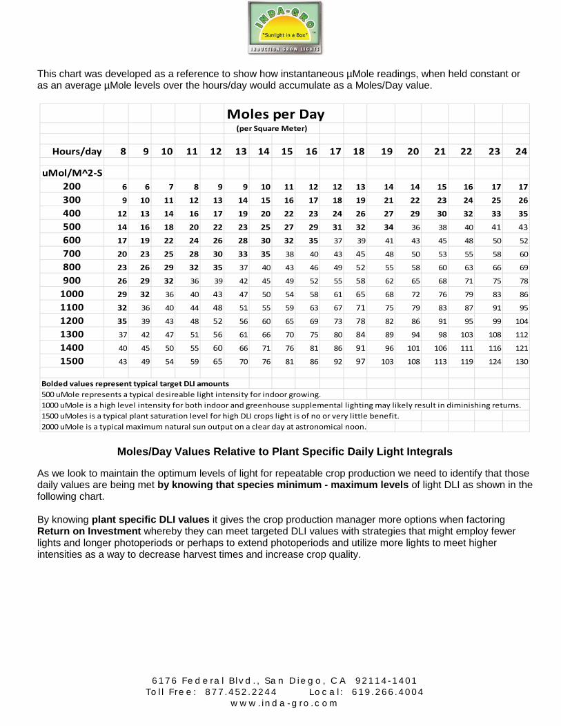
This chart was developed as a reference to show how instantaneous µMole readings, when held constant or as an average µMole levels over the hours/day would accumulate as a Moles/Day value.

Moles per Day (per Square Meter)

Hours/day 8 9 10 11 12 13 14 15 16 17 18 19 20 21 22 23 24

uMol/M^2-S200 6 6 7 8 9 9 10 11 12 12 13 14 14 15 16 17 17300 9 10 11 12 13 14 15 16 17 18 19 21 22 23 24 25 26400 12 13 14 16 17 19 20 22 23 24 26 27 29 30 32 33 35500 14 16 18 20 22 23 25 27 29 31 32 34 36 38 40 41 43600 17 19 22 24 26 28 30 32 35 37 39 41 43 45 48 50 52

700 20 23 25 28 30 33 35 38 40 43 45 48 50 53 55 58 60

800 23 26 29 32 35 37 40 43 46 49 52 55 58 60 63 66 69

900 26 29 32 36 39 42 45 49 52 55 58 62 65 68 71 75 78

1000 29 32 36 40 43 47 50 54 58 61 65 68 72 76 79 83 86

1100 32 36 40 44 48 51 55 59 63 67 71 75 79 83 87 91 95

1200 35 39 43 48 52 56 60 65 69 73 78 82 86 91 95 99 104

1300 37 42 47 51 56 61 66 70 75 80 84 89 94 98 103 108 112

1400 40 45 50 55 60 66 71 76 81 86 91 96 101 106 111 116 121

1500 43 49 54 59 65 70 76 81 86 92 97 103 108 113 119 124 130

Bolded values represent typical target DLI amounts500 uMole represents a typical desireable light intensity for indoor growing.1000 uMole is a high level intensity for both indoor and greenhouse supplemental lighting may likely result in diminishing returns.1500 uMoles is a typical plant saturation level for high DLI crops light is of no or very little benefit.2000 uMole is a typical maximum natural sun output on a clear day at astronomical noon.

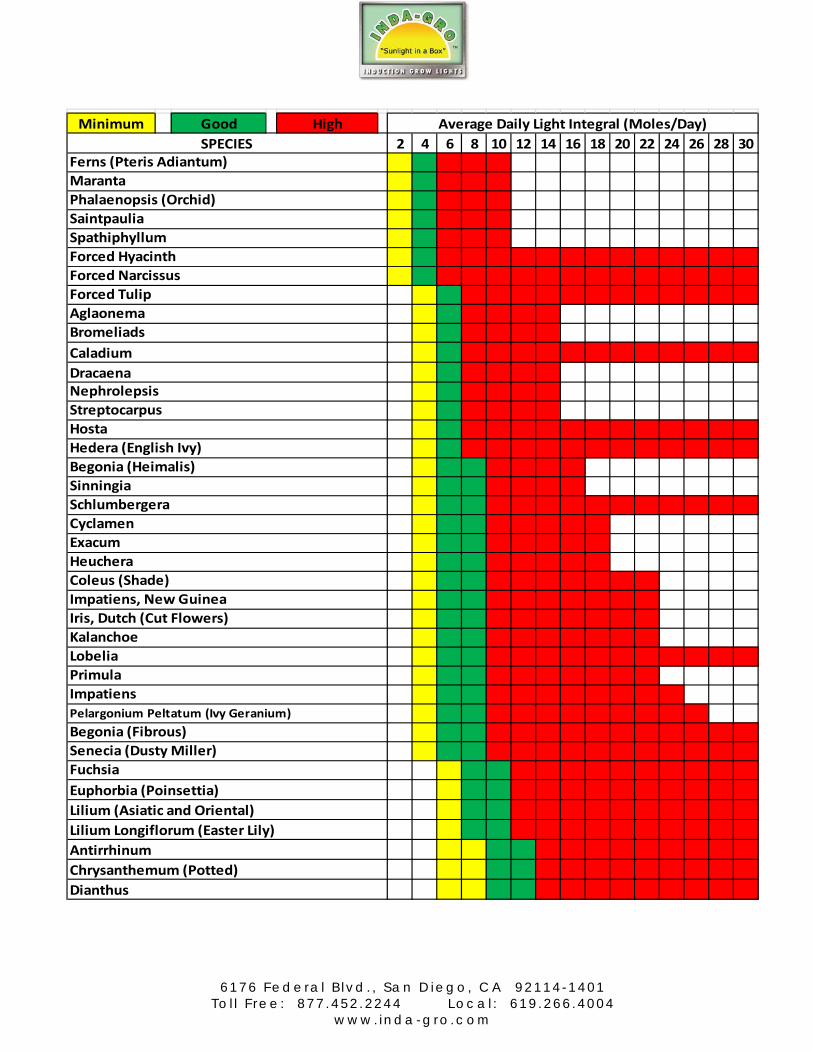
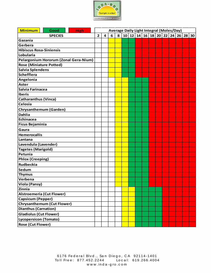
Moles/Day Values Relative to Plant Specific Daily Light Integrals

As we look to maintain the optimum levels of light for repeatable crop production we need to identify that those daily values are being met by knowing that species minimum - maximum levels of light DLI as shown in the following chart. By knowing plant specific DLI values it gives the crop production manager more options when factoring Return on Investment whereby they can meet targeted DLI values with strategies that might employ fewer lights and longer photoperiods or perhaps to extend photoperiods and utilize more lights to meet higher intensities as a way to decrease harvest times and increase crop quality.



Minimum Good High2 4 6 8 10 12 14 16 18 20 22 24 26 28 30

Ferns (Pteris Adiantum)SPECIES

Maranta

Average Daily Light Integral (Moles/Day)

Forced TulipAglaonemaBromeliadsCaladium

Phalaenopsis (Orchid)SaintpauliaSpathiphyllumForced HyacinthForced Narcissus

DracaenaNephrolepsisStreptocarpusHostaHedera (English Ivy)Begonia (Heimalis)SinningiaSchlumbergeraCyclamenExacumHeucheraColeus (Shade)Impatiens, New GuineaIris, Dutch (Cut Flowers)KalanchoeLobeliaPrimulaImpatiens Pelargonium Peltatum (Ivy Geranium)Begonia (Fibrous)

Lilium Longiflorum (Easter Lily)AntirrhinumChrysanthemum (Potted)Dianthus

Senecia (Dusty Miller)FuchsiaEuphorbia (Poinsettia)Lilium (Asiatic and Oriental)



Minimum Good High2 4 6 8 10 12 14 16 18 20 22 24 26 28 30

Chrysanthemum (Garden)DahliaEchinaceaFicus BejaminiaGaura

Salvia Farinacea

Average Daily Light Integral (Moles/Day)

IberisCatharanthus (Vinca)Celosia

HemerocallisLantanaLavendula (Lavender)Tagetes (Marigold)

Phlox (Creeping)Petunia

ZinniaAlstroemeria (Cut Flower)Capsicum (Pepper)Chrysanthemum (Cut Flower)

RudbeckiaSedumThymusVerbena

Dianthus (Carnation)Gladiolus (Cut Flower)Lycopersicon (Tomato)Rose (Cut Flower)

SPECIES GazaniaGerberaHibiscus Rosa-SiniensisLobulariaPelargonium Hororum (Zonal Gera-Nium)Rose (Miniature Potted)Salvia SplendensScheffleraAngeloniaAster

Viola (Pansy)



ElectroMagnetic Interference (EMI)

What is EMI? Electromagnetic Interference (EMI) is electrical or radio frequency noise that is unintentionally generated back onto the AC power or on the airwaves. Another term commonly used is Radio Frequency Interference (RFI) which is a subset of EMI, but specific to the frequencies used for radio transmissions. EMI is an unfortunate side effect of modern high speed digital signal processing. If it is incorporated into a high power application such as switching power supplies and digital lighting ballast we now have high frequency combined with high power and can generate significant EMI. Lighting is specifically an issue because it is present everywhere, our homes, scientific laboratories, hospitals, outdoors, etc. Further complicating the matter is the increased quantity of equipment that may be susceptible to EMI such as computers, cellular phones, precision laboratory equipment, hospital equipment, and implantable/portable medical equipment (pacemakers, defibrillators, infusion pumps, electric wheelchairs, and medical alert devices). One other area of concern is interference with communications on established bandwidths that are reserved for communications such as aviation, radio, TV, emergency, and military. How can EMI be dangerous? Some of the equipment functions and communications are absolutely critical and can be life endangering if they do not functioning properly. Obviously it is important for all of these devices to be able to work in harmony with each other while in relatively close proximity. To bring order to all of this chaos it is unavoidably necessary to have design standards and agencies to enforce it, thus the Federal Communications Commission (FCC) at least here in the U.S. The FCC does have standards that specifically address EMI for high frequency lighting, CFR Title 47 Part 18.303 and 18.307 for maximum allowable emitted and conducted EMI. For critical equipment there will also be susceptibility/immunity requirements to assure that they can tolerate some degree of EMI exposure. EMI concerns are the reason airlines would not allow passengers to use electronic devices at key points in the flight program. In the past there was a time period you were not allowed to use a cellular in a hospital and especially near critical areas such as the ICU. There have been many reports of EMI related incidents over the years, most 10 to 20 years ago when these issue where not as greatly appreciated as they are today. The key point with EMI is that with the increasing number and density of high frequency, high speed devices, be it wired or wireless, it makes these EMI standards and compliance to them paramount for everything to work in harmony. If manufacturers do not comply, the potential for unintended equipment interactions will exist. This creates an environment for which enforcement by government agencies such as the FCC is necessary to assure these EMI levels are not exceeded.



The Types of EMI and the Standards Manufacturers must Operate Within. EMITTED EMI (Ref. 18.303): These are emissions that are broadcast onto the airwaves. These types of emission are primarily a problem for communications devices as they can interfere with the airwave transmissions. Standard remedies are to use shielded cables and connections and a conductive Faraday cage containment of the device. FCC limits are specified at 30 meters, but the more common test distance is at 3 meters. Attenuation follows a 1/d relationship so testing at 3 meters will allow for 10 times the intensity that would be present at 30 meters (this is consistent with the FCC code). Lab reports are generally presented on a dB scale (dB = 20Log10(v/vref) rather than absolute voltage as specified by the FCC.

Emitted EMI Frequency Ranges Freq (MHz) FCC at 30 meters Test at 3 meters Test at 3 meters (µV/m) (µV/m) dB(µV/m) @ 1 µV/m ref Residential 30 - 88 10 100 40 88 - 216 15 150 43.5 216 - 1000 20 200 46.0 Commercial 30 - 88 30 300 49.5 88 - 216 50 500 54 216 - 1000 70 700 56.9 When equipment is tested for Emitted EMI the blue line shows the level of EMI it produced. The stepped lines correspond to the allowable limit frequency values as shown above. In this case the equipment would be suitable for either a residential or commercial installation as none of the blue line values exceed the allowable limits.



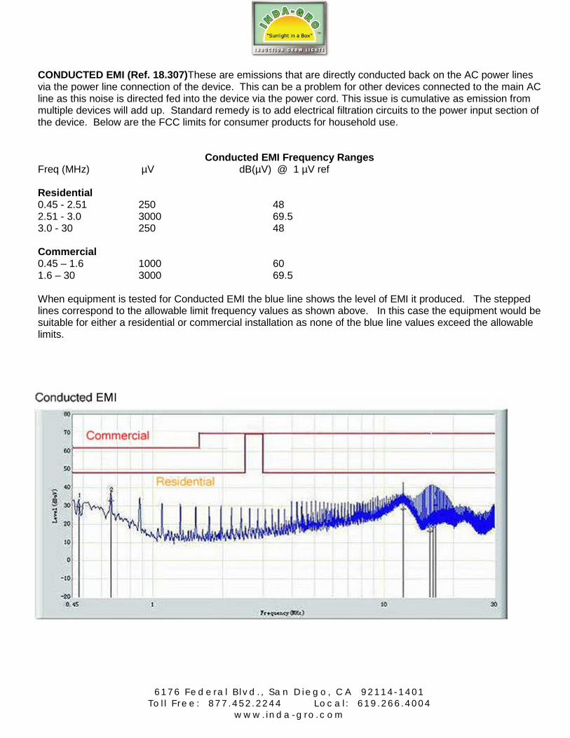
CONDUCTED EMI (Ref. 18.307)These are emissions that are directly conducted back on the AC power lines via the power line connection of the device. This can be a problem for other devices connected to the main AC line as this noise is directed fed into the device via the power cord. This issue is cumulative as emission from multiple devices will add up. Standard remedy is to add electrical filtration circuits to the power input section of the device. Below are the FCC limits for consumer products for household use.

Conducted EMI Frequency Ranges Freq (MHz) µV dB(µV) @ 1 µV ref Residential 0.45 - 2.51 250 48 2.51 - 3.0 3000 69.5 3.0 - 30 250 48 Commercial 0.45 – 1.6 1000 60 1.6 – 30 3000 69.5 When equipment is tested for Conducted EMI the blue line shows the level of EMI it produced. The stepped lines correspond to the allowable limit frequency values as shown above. In this case the equipment would be suitable for either a residential or commercial installation as none of the blue line values exceed the allowable limits.



I want to calculate the intensity of light at the canopy.

To what degree do the laws of Inverse Square apply to artificial grow lighting layouts?

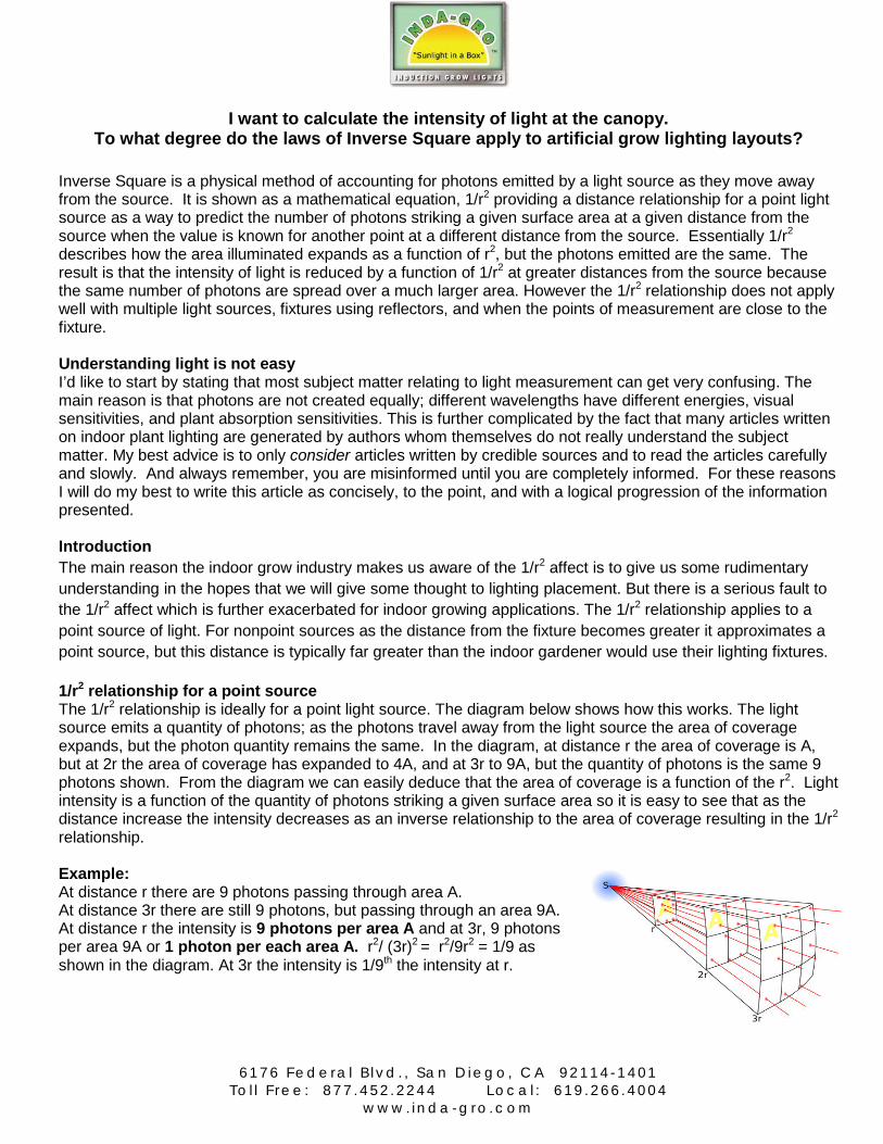
Inverse Square is a physical method of accounting for photons emitted by a light source as they move away from the source. It is shown as a mathematical equation, 1/r2 providing a distance relationship for a point light source as a way to predict the number of photons striking a given surface area at a given distance from the source when the value is known for another point at a different distance from the source. Essentially 1/r2 describes how the area illuminated expands as a function of r2, but the photons emitted are the same. The result is that the intensity of light is reduced by a function of 1/r2 at greater distances from the source because the same number of photons are spread over a much larger area. However the 1/r2 relationship does not apply well with multiple light sources, fixtures using reflectors, and when the points of measurement are close to the fixture. Understanding light is not easy I’d like to start by stating that most subject matter relating to light measurement can get very confusing. The main reason is that photons are not created equally; different wavelengths have different energies, visual sensitivities, and plant absorption sensitivities. This is further complicated by the fact that many articles written on indoor plant lighting are generated by authors whom themselves do not really understand the subject matter. My best advice is to only consider articles written by credible sources and to read the articles carefully and slowly. And always remember, you are misinformed until you are completely informed. For these reasons I will do my best to write this article as concisely, to the point, and with a logical progression of the information presented. Introduction The main reason the indoor grow industry makes us aware of the 1/r2 affect is to give us some rudimentary understanding in the hopes that we will give some thought to lighting placement. But there is a serious fault to the 1/r2 affect which is further exacerbated for indoor growing applications. The 1/r2 relationship applies to a point source of light. For nonpoint sources as the distance from the fixture becomes greater it approximates a point source, but this distance is typically far greater than the indoor gardener would use their lighting fixtures. 1/r2 relationship for a point source The 1/r2 relationship is ideally for a point light source. The diagram below shows how this works. The light source emits a quantity of photons; as the photons travel away from the light source the area of coverage expands, but the photon quantity remains the same. In the diagram, at distance r the area of coverage is A, but at 2r the area of coverage has expanded to 4A, and at 3r to 9A, but the quantity of photons is the same 9 photons shown. From the diagram we can easily deduce that the area of coverage is a function of the r2. Light intensity is a function of the quantity of photons striking a given surface area so it is easy to see that as the distance increase the intensity decreases as an inverse relationship to the area of coverage resulting in the 1/r2 relationship.

Example: At distance r there are 9 photons passing through area A. At distance 3r there are still 9 photons, but passing through an area 9A. At distance r the intensity is 9 photons per area A and at 3r, 9 photons per area 9A or 1 photon per each area A. r2/ (3r)2 = r2/9r2 = 1/9 as shown in the diagram. At 3r the intensity is 1/9th the intensity at r.



Nonpoint source affects If you have ever taken light intensity measurements under your grow light you very likely did not get a 1/r2 relationship, but likely somewhere in between a 1/r and a 1/r2 relationship. This has nothing to do with using a proper quantum meter or a standard light meter, but a result of the light fixture not being a true point source. As you get further from the lamp it starts to approximate a point source. An industry rule of thumb is at a distance of 5 times the largest dimension of the fixture the 1/r2 relationship starts to hold. The largest dimension would only include the parts that actually emit light from the fixture. This would include all reflector material, but not any housing materials in areas that light is not emitted.

If the largest dimension was 2 feet, then 5 X 2 feet would be 10 feet, so this is the minimum point that the fixture starts to approximate a point source and the 1/r2 relationship starts to hold. But keep in mind this is only for measurements that are all taken from a distance of 10 feet or greater.

Real world light fixtures behave more like multiple point sources in close proximity to each other. LED panels are very much that with each individual LED effectively a point source. A lighting fixture will approximate a point source, but only at large distance, much higher than most indoor gardeners would place their lamps. Reflectors in particular skew the 1/r2 affect because they bounce photons at radically different angles than the photons emitted directly from the lamp. A reflected photon that could not be detected at a centered position very close to the lamp (point 1) may be detected at the same centered position, but at a greater distance from the lamp (point 2). This is a result of a side reflector bouncing a photon back toward the center at an angle. In the previous example for a point source, the photons only disperse from the center outward. The reflector can bounce photons from one side back toward the center and across to the other side. This is the major contributor in the breakdown of the 1/r2 relationship at close distances.

In the case of an LED panel, as you take measurements at different distance from the panel, the photons emitted by the LED directly above the measure point are dispersing from the center. But at the same time the LEDs located off center are emitting photons that may not be detected at a center point close to the panel (point 1), but will be detected at the same center point at a distance further from the panel (point 2).



Measurements taken near the light fixture are capturing photons emitted from multiple points at greatly varying angles. As the point of measurement is taken from greater distances, these angles are reduced and are more similar to each other and this is why it starts to approximate a point source at the greater distances.

Conclusion 1/r2 is not a critical phenomenon to be overly concerned with in your light set up. It is good to understand it as it will help in understanding any intensity measurements you take. The main objective is to place your light fixtures and the height of the fixture such that it projects the footprint needed while minimizing the light overspray past the crops. Most all of us will find this balance by experimentation and not by performing calculations with parameters that the manufacturers do not provide anyway.

What should I be looking for in a grow light reflector? Reflectors in lighting fixtures perform 2 major functions, redirecting light downward from behind and aside the lamp, and distributing the light intensity downward in the desired footprint pattern and evenness. A third, but lesser function is helping with heat dissipation. While it is well understood that a good reflector design is important it is not always apparent that all manufacturers put out the proper effort or that end users choose properly for their application. Redirecting Light Redirecting light back toward the crop is the most obvious and basic function of a reflector. With the exception of LED units all lamp technologies emit light in all direction. Even if 120 degree beam pattern were desirable then about 2/3 of the emitted light is going the wrong direction and needs to be redirected toward the desired area of illumination. In this respect the most important factor is getting as much of the light as possible redirected forward with as few reflector bounces as possible. The main trick is to avoid getting light trapped deep behind the lamp and reflecting light back toward the lamp. Distributing Light over the Footprint A good reflector design will ultimately result in a specific footprint shape with as much evenness of intensity as possible. This is the more difficult task requiring real engineering and ingenuity and the final result will never be ideal, but only as good as the designer. Lamps tend to project oval or round footprints, but the most practical use is to have a rectangular or square footprint. The challenge is to redistribute light to fill in these corners. For grow applications this is a unique challenge since the requirement for a relatively even intensity distribution is not very critical for most other lighting applications. Specular vs. Diffusive Reflectors This seems to be a topic for some discussion, but there is no clear answer as to whether one is superior to the other. The real issue is most likely to use the style that best suits the particular application and need. This may actually result in a mixing of the two styles. Diffusive will likely result in additional reflections and greater reflective losses. If the light is buried behind the lamp then diffusive may be the best bet to recover some of the light, but at that point perhaps a repositioning of the lamp may be justified. Diffusive can also help even out the distribution of light over the desired footprint. Generally when light can be easily reflected in a desirable direction then specular likely makes the most since and will be the most efficient since the reflections will be more direct.



No Effort Designs When looking at a reflector it is pretty easy to pick out the units for which no real effort is made in the design. These manufacturers are just attempting to reflect the back and side light with no effort to aim it in any particular direction. Often they do not even do the best job of recovering as much of this light as they could. Reflectors that simply follow the straight angular contours of the hood are an obvious sign of this. Some hoods are just painted with a highly reflected paint. There are some hoods which themselves are shape as a good reflector design so they would not be included in this group. If by appearance it is obvious that little to no effort was put into the design that is likely the case. The images below shows how two different manufacturers approach reflector designs. The fixture on the left is manufactured by Inda-Gro Induction lighting (MSRP $795.00) weighs in @ 14lbs and uses a separate specular reflector material from the housing. This reflector is both highly reflective and specifically fabricated with geometry to maximize redirection of the photons that would be lost from the rear of the lamp and from between the opposing tubes back towards the canopy. The fixture on the right is manufactured by the iGrow company (MSRP $1,200.00) weighs in @ 38lbs and utilizes the hood as a diffusive reflector. This is an inexpensive and unimaginitive use of the lamp technology as the reflective surfaces are not highly reflective and are too far away from the lamp which is lost energy as it meets that surface and is redirected. The other issue you’ll note with the reflective characteristics of the iGrow light is that the interior ends are not angled to project light downwards. They are simply flat edges at right angles to the lamp surface. Consequently the Inda-Gro will emit light intensity 20-30% higher than the iGrow over a 4 x 4 area with their reflector material and design over painted metal surfaces that lack the geometric properties necessary to optimize area coverage.



A Manufacturers Perspective as to the Future of Artificial Grow Lighting Systems

We are of the opinion that the best light to grow plants is the sun, always has been, always will be. The reason: 4 billion years of symbiotic evolution. As engineers we are continuously looking to increase artificial plant lighting efficiencies and should remember that our planet has supported a wide variety of plant species, fed by sunlight, for nearly 4 billion years. The plant/sun relationship is both a dynamic and an intimate one and it is incumbent upon us to take into careful consideration precisely what aspects of this relationship have led to successful outdoor crop production and bring those qualities to our indoor lighting designs. For us to grow plants that are healthy, nutrient dense and prolific we must approach artificial lamp design starting with an understanding of natural conditions first and avoid falling victim to anthropocentrism which is a human condition where we have a tendency to regard ourselves as being at the center of the universe. This can lead to myopic close mindedness and an inability to grasp the ‘big picture’. Combining a pinch of anthropocentrism with a ‘this is the way we’ve always done it’ mentality can seriously get in the way of advancing next generation artificial plant lighting systems. Manmade lamps can never cost effectively recreate the sun in terms of power consumption and broad spectrums such that indoor gardening would be economically feasible with such a lamp. Sacrifices must be made. When considering those sacrifices the objective would be to reduce those spectrums that are less likely to have the least negative impact on plant development, but not entirely eliminate those spectrums from a lamp that emits broad PAR spectrums similar to what plants would be exposed to under natural sunlight conditions. While we have benefitted from research that has given us a greater understanding the complex interplay between highly evolved plant system and the sun, we continue to learn more about plant photochemical responses that will serve to benefit our future artificial lighting designs. Armed with the knowledge gained from this research and driven by rising utility rates, engineers have been on a quest to develop lamp technologies that deliver intensities and PAR spectrums which are energy efficient, long life/low depreciation, stable spectrum and afford low thermal contribution while optimizing crop production values. That pursuit has led to designing lamps that reduced, or in the case of many LED panels, eliminating, what was considered “wasted" wavelengths while those wavelengths associated with the greatest response are emphasized. In seeking to ‘out engineer’ nature with artificial grow lights that are energy efficient and improve plant response, one approach has been to reduce the importance of the natural symbiosis which occurs between broad spectrum sunlight and plants, by attempting to force plant development with specific, narrow band, wavelengths which research has shown proves beneficial during specific stages of growth. That research has led to a widely accepted, market driven approach to artificial plant lighting that has relied plants favorable response to red light during their bloom phase and preference to blue light during their vegetative phase. In plant lighting design this has become accepted doctrine and has taken on the look of law, however these conclusions were obtained from laboratory trials in which the chlorophyll response was measured against a wide spectrum of light frequencies and those with the highest response were considered photosynthetically active and the rest considered superfluous. This approach, while good for selling a wide variety of lamp types, neglects to take into consideration the big picture design that would intuitively suggest that plants exposed to broad spectrum wavelengths are more likely to respond similarly to plants that had been grown under broad spectrum sunlight conditions. In many of the LED panel designs this is epitomized to the extreme whereby some panels will utilize all RED diodes, all BLUE diodes or a hybrid matrix of the two virtually ignoring what they believe to be the ‘less important’ wavelengths then monitor the plants photosynthetic response where any increase in said response is considered a victory. We feel this approach is myopic and does not adequately address the overall health of the plant.



When considering which artificial lighting technology to install in your indoor garden, keep in mind that the light you choose affects every aspect of your system: water temperature, air temperature, evapotranspiration rates, RH, VPD, rate of CO2 uptake, DO levels, symbiotic bacterial densities, disease resistance, pest resistance, canopy biomass, root biomass, fruit and flower production, nutrient density, brix levels, the list is virtually endless. In sunlight conditions, where the plants receive broad spectrums throughout the entire growth cycle, successful plant development is achieved through the processes of natural equilibrium whereby all of these elements come together to benefit overall plant health. As further debate will continue to swirl over the merits of broad versus narrow spectrum plant lighting it is worth noting that with nearly 400,000 different plant species on this planet, from greatly varied regions: Why would one attempt to apply a generalized model to such a disparate population? In designing and promoting stage specific lamp solutions we have essentially divorced ourselves from the natural cycle and consequently blinded our ability to see the elegant broad spectrum solution that nature has provided our plants. Greenhouse gardeners take advantage of that evolution in that their crops do rely on sunlight as the primary light source. When regions and time of year require that supplemental lighting systems be used to augment insufficient levels of sunlight for a particular crop, the greenhouse gardener will also be interested in finding the latest technologies that meld energy efficiencies, crop repeatability, reduced time to harvest, tighter internodal spacing, increased fruit and flower sizes, and higher quality for their crops. For a side by side comparison of plants being grown in a greenhouse with sunlight only verses plants grown with sunlight/supplemental lighting systems see the links posted on the references page. High Intensity Discharge or HID lighting systems have been in use as artificial lighting systems in both greenhouse and indoor gardens for the last 40 years. What separates the greenhouse grower from the indoor grower is that they will rely on sunlight for the primary light source and the supplemental lighting system they select should deliver the spectrums the crops require, and not waste precious energy by being on or running at higher intensities when natural light conditions preclude the need for the supplemental lighting to be running. A historic limitation with any HID systems is that they require long restrike times once turned off. A cooling off period to full intensity often takes 20 minutes or more. This type of technology does not lend itself to microprocessor based control systems whereby the light output levels may be instantly tuned on or off and then raised or lowered as ambient conditions would dictate. Ultimately it is through lighting and control systems that do offer wider control capabilities which will enable the greenhouse gardener to meet their crops daily light integrals without consuming energy unnecessarily by doing so. As an industry we have a moral responsibility to advance those technologies that reduce waste and outperform prior generation technologies. Yes, it’s a daunting task attempting to identify all the collateral variables that are either directly or indirectly influenced by the artificial light source but assuredly, all the hard work is worth it as a thorough understanding of these underlying relationships will result in unprecedented yields and unrivaled overall quality.

By Darryl Cotton, President Inda-Gro Lighting Systems



References: Supplemental Greenhouse Lighting by Cotton and Hagler http://www.inda-gro.com/pdf/Inda-GroGreenhouseReport.pdf Photosynthesis by Rabinowitch and Govindjee http://www.life.illinois.edu/govindjee/photosynBook.html Plant Growth and Flowering by King and Bagnall http://www.controlledenvironments.org/Light1994Conf/2_4_King/King%20text.htm Understanding Phytochrome by Koning http://plantphys.info/plant_physiology/phytochrome.shtml Energy Consumption for Indoor Commercial Cannabis by Mills http://evan-mills.com/energy-associates/Indoor_files/Indoor-cannabis-energy-use.pdf We apologize for any broken links you might encounter. At the time of this writing they were all available.

Thank you for taking the time to read and explore the information we have put forth in this document. We hope you have found it useful and will use it for future reference. This document has not been copyrighted and may be used in whole or in part for reprint or distribution. Date of Document 12-20-13 (Version 2.3)

http://www.inda-gro.com/pdf/Inda-GroGreenhouseReport.pdf

http://www.life.illinois.edu/govindjee/photosynBook.html

http://www.controlledenvironments.org/Light1994Conf/2_4_King/King%20text.htm

http://plantphys.info/plant_physiology/phytochrome.shtml

http://evan-mills.com/energy-associates/Indoor_files/Indoor-cannabis-energy-use.pdf

Measuring Plant Lighting - Inda-Gro · Measuring Plant Lighting There are a number of ways to...

Documents

Transcript of Measuring Plant Lighting - Inda-Gro · Measuring Plant Lighting There are a number of ways to...