Measuring Impedance Across the Channel of a Biodevice
23
Measuring Measuring Impedance Across Impedance Across the Channel of a the Channel of a Biodevice Biodevice Presented by: Kaidi He Presented by: Kaidi He August 24, 2007 August 24, 2007 Mentors: Prof. Reginald Mentors: Prof. Reginald Penner Penner Li-Mei Yang Li-Mei Yang
description
Measuring Impedance Across the Channel of a Biodevice. Presented by: Kaidi He August 24, 2007 Mentors: Prof. Reginald Penner Li-Mei Yang. Outline. Project Overview Methods Device Fabrication Experimental Setup Procedures Data and Analysis Conclusion. I. Project Overview. - PowerPoint PPT Presentation
Transcript of Measuring Impedance Across the Channel of a Biodevice

Measuring Impedance Measuring Impedance Across the Channel of a Across the Channel of a
Biodevice Biodevice
Presented by: Kaidi HePresented by: Kaidi HeAugust 24, 2007August 24, 2007
Mentors: Prof. Reginald Penner Mentors: Prof. Reginald Penner Li-Mei YangLi-Mei Yang
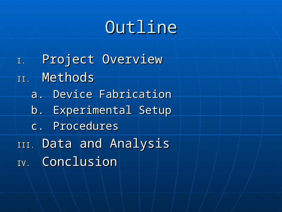
OutlineOutline
I.I. Project OverviewProject Overview
II.II. MethodsMethodsa.a. Device FabricationDevice Fabrication
b.b. Experimental SetupExperimental Setup
c.c. ProceduresProcedures
III.III. Data and AnalysisData and Analysis
IV.IV. ConclusionConclusion

I. Project OverviewI. Project Overview
Measure impedance across Measure impedance across the channel of a biodevice the channel of a biodevice for different channel widths for different channel widths exposed to various exposed to various concentrationsconcentrations
Construct a calibration curveConstruct a calibration curve
Courtesy of Prof. Penner

SU8
Glass
Au
SU8
Au
ExposureDevelopment
Au etch
II. Methods, (a) Device FabricationII. Methods, (a) Device Fabrication
A.B.
A.
B.
Courtesy of Li-Mei Yang
SU-8
Au
glassAu
SU-8

Original:Original:• NickelNickel• Wire attachmentsWire attachments• Silver contactsSilver contacts
Final:Final:• Gold with silver Gold with silver
contactscontacts
S
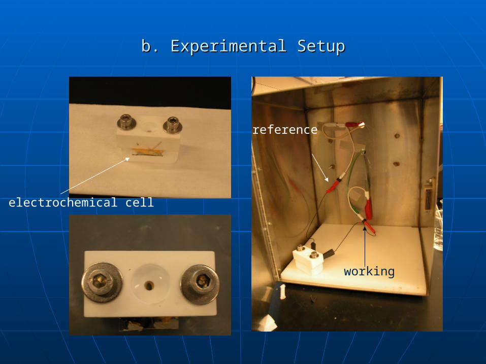
b. Experimental Setupb. Experimental Setup
electrochemical cell
reference
working
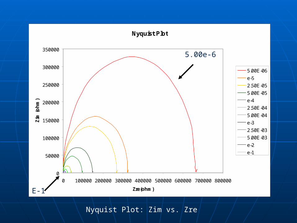
Nyquist Plot
0
50000
100000
150000
200000
250000
300000
350000
0 100000 200000 300000 400000 500000 600000 700000 800000
Zre(ohm)
Zim
(o
hm
)
5.00E-06
e-5
2.50E-05
5.00E-05
e-4
2.50E-04
5.00E-04
e-3
2.50E-03
5.00E-03
e-2
e-1
5.00e-6
E-1
Nyquist Plot: Zim vs. Zre

Bode Plot
0
100000
200000
300000
400000
500000
600000
700000
800000
0.1 1 10 100 1000 10000 100000 1000000
Freq (hz)
Zre
(o
hm
)
5.00E-06
e-5
2.50E-05
5.00E-05
e-4
2.50E-04
5.00E-04
e-3
2.50E-03
5.00E-03
e-2
e-1
Bode Plot: Zre, Zim, phase angle vs. Frequency

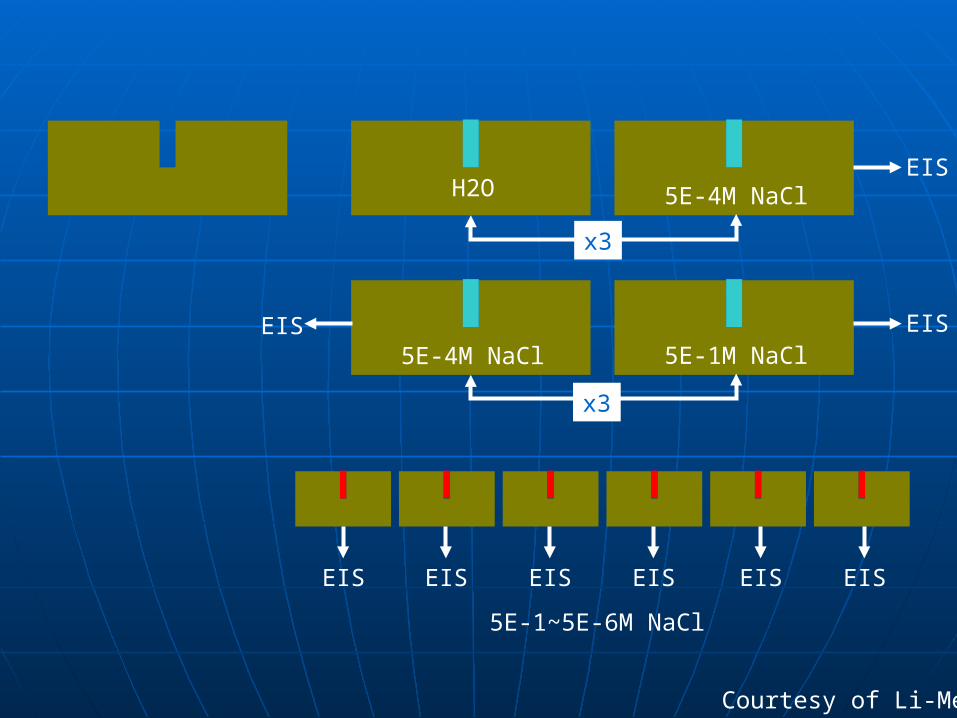
5E-4M NaCl 5E-1M NaClEISEIS
x3
H2O 5E-4M NaClEIS
x3
0.1 – 5e-6 M NaCl
EIS EIS EIS EIS EIS EIS
(3) Procedures(3) Procedures
Courtesy of Li-Mei
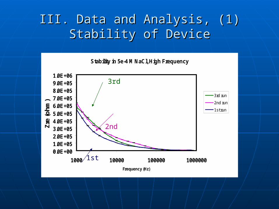
III. Data and Analysis, (1) Stability of DeviceIII. Data and Analysis, (1) Stability of Device
Stability in 5e-4 M NaCl, High Frequency
0.0E+001.0E+052.0E+053.0E+054.0E+055.0E+056.0E+057.0E+058.0E+059.0E+051.0E+06
1000 10000 100000 1000000
Frequency (Hz)
Zre
(oh
m)
3rd run
2nd run
1st run
1st
2nd
3rd

5E-4M NaCl 5E-1M NaClEISEIS
x3
H2O 5E-4M NaClEIS
x3
5E-1-5E-6M NaCl
EIS EIS EIS EIS EIS EIS
Courtesy of Li-Mei
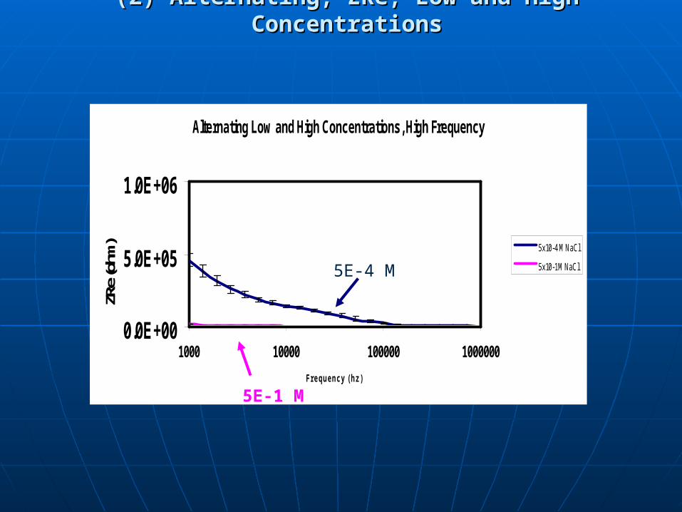
Alternating Low and High Concentrations, High Frequency
0.0E+00
5.0E+05
1.0E+06
1000 10000 100000 1000000
Frequency (hz)
ZRe (
ohm) 5x10⁻⁴ M NaCl
5x10⁻¹ M NaCl5E-4 M
5E-1 M
(2) Alternating, ZRe, Low and High Concentrations(2) Alternating, ZRe, Low and High Concentrations
5E-4 M
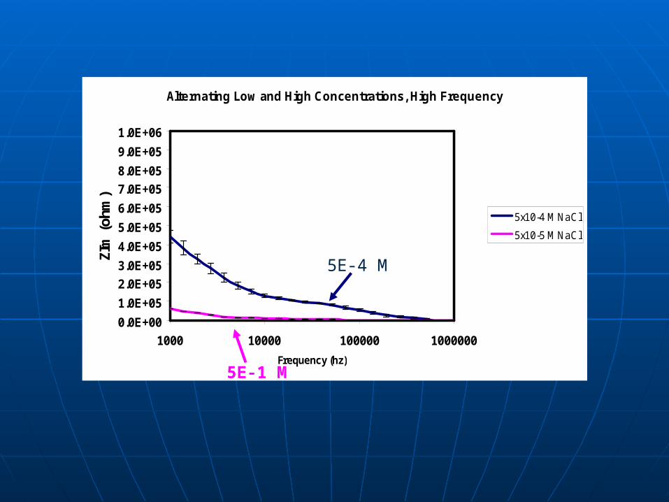
Alternating Low and High Concentrations, High Frequency
0.0E+00
1.0E+05
2.0E+05
3.0E+05
4.0E+05
5.0E+05
6.0E+05
7.0E+05
8.0E+05
9.0E+05
1.0E+06
1000 10000 100000 1000000
Frequency (hz)
ZIm
(oh
m)
5x10⁻⁴ M NaCl
5x10⁻⁵ M NaCl
5E-4 M
5E-1 M

ZRe at Selected Frequencies
0.0E+00
2.0E+07
4.0E+07
6.0E+07
8.0E+07
1.0E+08
1.2E+08
1.4E+08
1.6E+08
1.8E+08
2.0E+08
5x10^-4 5x10^-1 5x10^-4 5x10^-1 5x10^-4 5x10^-1
ZR
e (o
hm
)
0.1 hz
10 hz
100 hz
1000 hz
10 4̂ hz
10 5̂ hz
1. Low concentration, more noise2. Low frequency, more noise
ZRe at Selected Frequencies
0.0E+00
1.0E+06
2.0E+06
3.0E+06
4.0E+06
5.0E+06
6.0E+06
7.0E+06
5x10^-4 5x10^-1 5x10^-4 5x10^-1 5x10^-4 5x10^-1
ZR
e (o
hm
)
10 hz
100 hz
1000 hz
10 4̂ hz
10 5̂ hz
5E-4M NaCl 5E-1M NaClEISEIS
x3
H2O 5E-4M NaClEIS
x3
5E-1~5E-6M NaCl
EIS EIS EIS EIS EIS EIS
Courtesy of Li-Mei

(3) Random Sampling(3) Random Sampling
• As expected, increasing concentration results in decreasing resistance
ZRe at Selected Concentrations, High Frequency
0.0E+00
1.0E+05
2.0E+05
3.0E+05
4.0E+05
5.0E+05
6.0E+05
1000 10000 100000 1000000
Frequency (hz)
ZR
e (
oh
m)
5x10 -̂6
5x10 -̂5
5x10 -̂4 (2)
5x10 -̂4 (1)
5x10 -̂4 (3)
5x10 -̂3
5x10 -̂2
5x10 -̂1
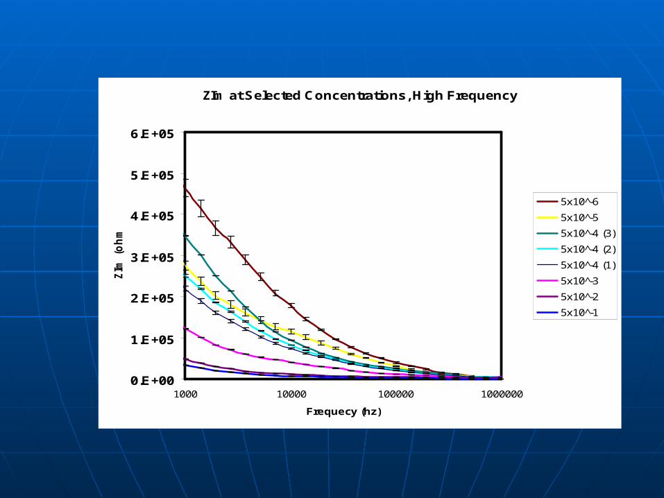
ZIm at Selected Concentrations, High Frequency
0.E+00
1.E+05
2.E+05
3.E+05
4.E+05
5.E+05
6.E+05
1000 10000 100000 1000000
Frequecy (hz)
ZIm
(o
hm
)
5x10 -̂6
5x10 -̂5
5x10 -̂4 (3)
5x10 -̂4 (2)
5x10 -̂4 (1)
5x10 -̂3
5x10 -̂2
5x10 -̂1
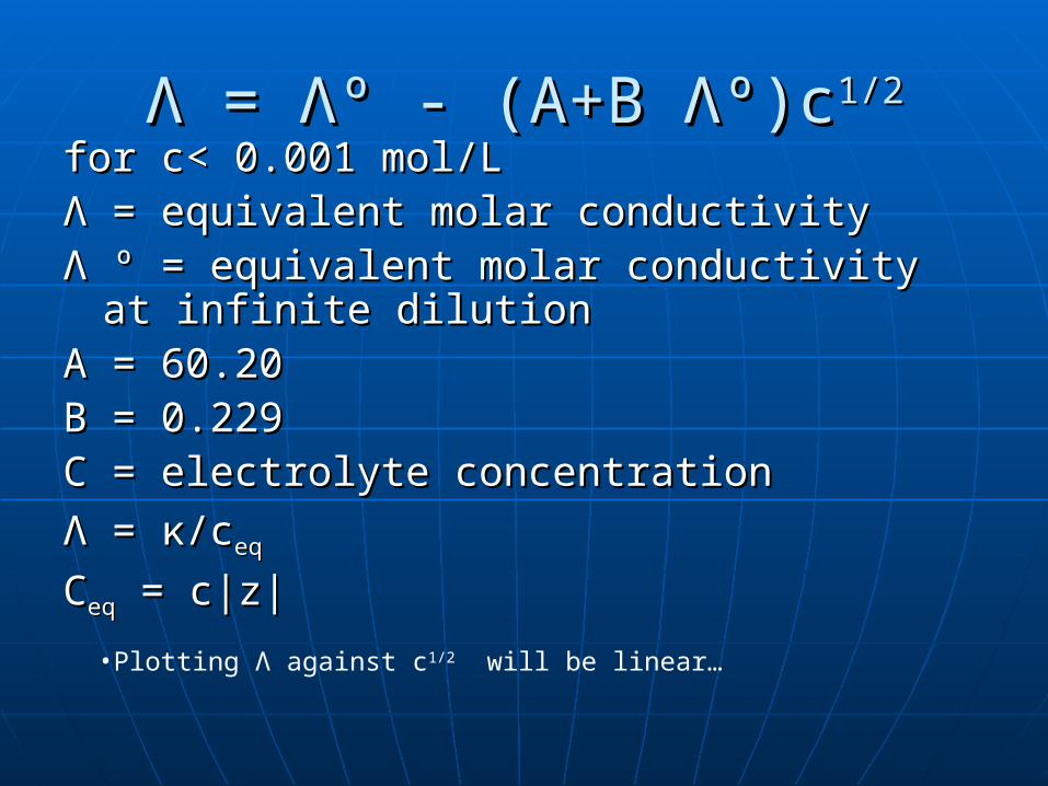
Λ = Λº - (A+B Λº)cΛ = Λº - (A+B Λº)c1/21/2
for c< 0.001 mol/Lfor c< 0.001 mol/LΛ = equivalent molar conductivityΛ = equivalent molar conductivityΛ º = equivalent molar conductivity at Λ º = equivalent molar conductivity at
infinite dilutioninfinite dilutionA = 60.20A = 60.20B = 0.229B = 0.229C = electrolyte concentrationC = electrolyte concentration
Λ = κ/cΛ = κ/ceqeq
CCeqeq = c|z| = c|z|
•Plotting Λ against c1/2 will be linear…

Sample Data Set, 500 micronSample Data Set, 500 micronLog 1/(zre*c) vs. Log c1/2
y = -1.4527x - 4.5001
R2 = 0.9956
-4.5
-4
-3.5
-3
-2.5
-2
-1.5
-1
-0.5
0
-3 -2.5 -2 -1.5 -1 -0.5 0
log c1/2
log
1/(
zre*
c)
1000 hz
Linear (1000 hz)

Sample Data Set, 1 mm deviceSample Data Set, 1 mm devicelog 1/(zre*c) vs. log c1/2
y = -1.3475x - 4.1073
R2 = 0.9919
-4.5
-4
-3.5
-3
-2.5
-2
-1.5
-1
-0.5
0
-3 -2.5 -2 -1.5 -1 -0.5 0
log c1/2
log
1/(
zre*
c)
1000 hz
Linear (1000 hz)

Sample Data Set, 3.5 mm deviceSample Data Set, 3.5 mm device
Log 1/(zre*c) vs. Log c1/2
y = -1.6014x - 4.8176
R2 = 0.9483
-5
-4.5
-4
-3.5
-3
-2.5
-2
-1.5
-1
-0.5
0
-3 -2.5 -2 -1.5 -1 -0.5 0
log c1/2
log
1/(z
re*c
)
1000 hz
Linear (1000 hz)

IV. ConclusionIV. Conclusion
We have achieved our goal of constructing a We have achieved our goal of constructing a calibration curve which will allow us to know calibration curve which will allow us to know concentration with a device of given channel concentration with a device of given channel width and impedance across the channelwidth and impedance across the channel
With photolithography, we are able to construct With photolithography, we are able to construct miniaturized conductivity cells quantitatively miniaturized conductivity cells quantitatively follow the Debye-Huckel-Onsanger Equation and follow the Debye-Huckel-Onsanger Equation and operate best at large interelectrode spacingsoperate best at large interelectrode spacings
This most likely will lead to their functioning as This most likely will lead to their functioning as biosensor transducers in the futurebiosensor transducers in the future

AcknowledgmentsAcknowledgments
Thank you to Prof. Penner, Li-Mei Thank you to Prof. Penner, Li-Mei Yang, Keith Donovan, Travis Kruse, Yang, Keith Donovan, Travis Kruse, Dat Hoang, Said Shokair, IM-SURE, Dat Hoang, Said Shokair, IM-SURE, and NSF for their guidance and and NSF for their guidance and support support