
Measuring Impact II – Non-experimental...
43
Measuring Impact II – Non-experimental Methods David Evans, World Bank Dakar, Senegal Wednesday, October 2, 2013
Transcript of Measuring Impact II – Non-experimental...

Measuring Impact II – Non-experimental Methods
David Evans, World Bank
Dakar, Senegal Wednesday, October 2, 2013

Lessons from Yesterday o What’s a counterfactual?

Lessons from Yesterday o Why is Before-After an incorrect
counterfactual?
o Why is Enrolled-Not Enrolled an incorrect counterfactual?

Lessons from Yesterday o What does randomization deliver?
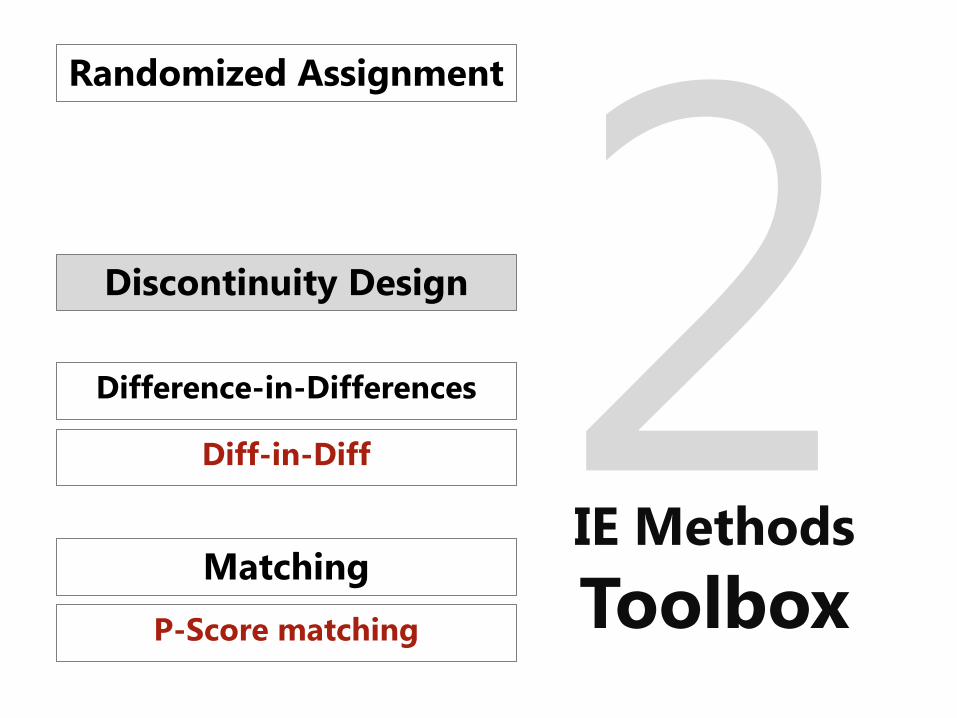
IE Methods Toolbox
Randomized Assignment
Discontinuity Design
Diff-in-Diff
Difference-in-Differences
P-Score matching
Matching

Discontinuity Design
Anti-poverty Programs
Pensions
Education
Agriculture
Many social programs select beneficiaries using an index or score:
Targeted to households below a given poverty index/income
Targeted to population above a certain age
Scholarships targeted to students with high scores on standarized text
Fertilizer program targeted to small farms less than given number of hectares)

Example: Effect of fertilizer program on agriculture production
Improve school attendance for poor students Goal
o Households with a score (Pa) of assets ≤50 are poor o Households with a score (Pa) of assets >50 are not poor
Method
Poor households receive scholarships to send children to school
Intervention

Regression Discontinuity Design-Baseline
Not eligible
Eligible

Regression Discontinuity Design-Post Intervention
IMPACT

Case 5: Discontinuity Design We have a continuous eligibility index with a defined cut-off o Households with a score ≤ cutoff are eligible o Households with a score > cutoff are not eligible o Or vice-versa Intuitive explanation of the method: o Units just above the cut-off point are very similar to
units just below it – good comparison. o Compare outcomes Y for units just above and below the
cut-off point.

Case 5: Discontinuity Design Eligibility for Progresa is based on national poverty index
Household is poor if score ≤ 750
Eligibility for Progresa: o Eligible=1 if score ≤ 750 o Eligible=0 if score > 750
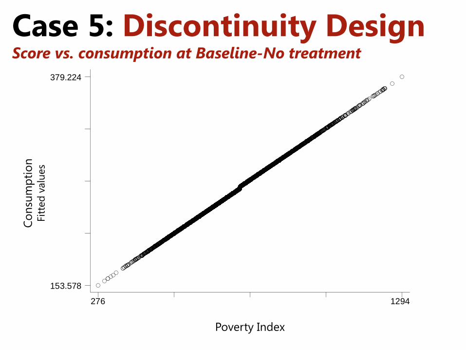
Case 5: Discontinuity Design Score vs. consumption at Baseline-No treatment
Fitte
d va
lues
puntaje estimado en focalizacion276 1294
153.578
379.224
Poverty Index
Cons
umpt
ion
Fitt
ed v
alue
s

Fitte
d va
lues
puntaje estimado en focalizacion276 1294
183.647
399.51
Case 5: Discontinuity Design Score vs. consumption post-intervention period-treatment
(**) Significant at 1%
Cons
umpt
ion
Fitt
ed v
alue
s
Poverty Index
30.58** Estimated impact on consumption (Y) | Multivariate Linear Regression
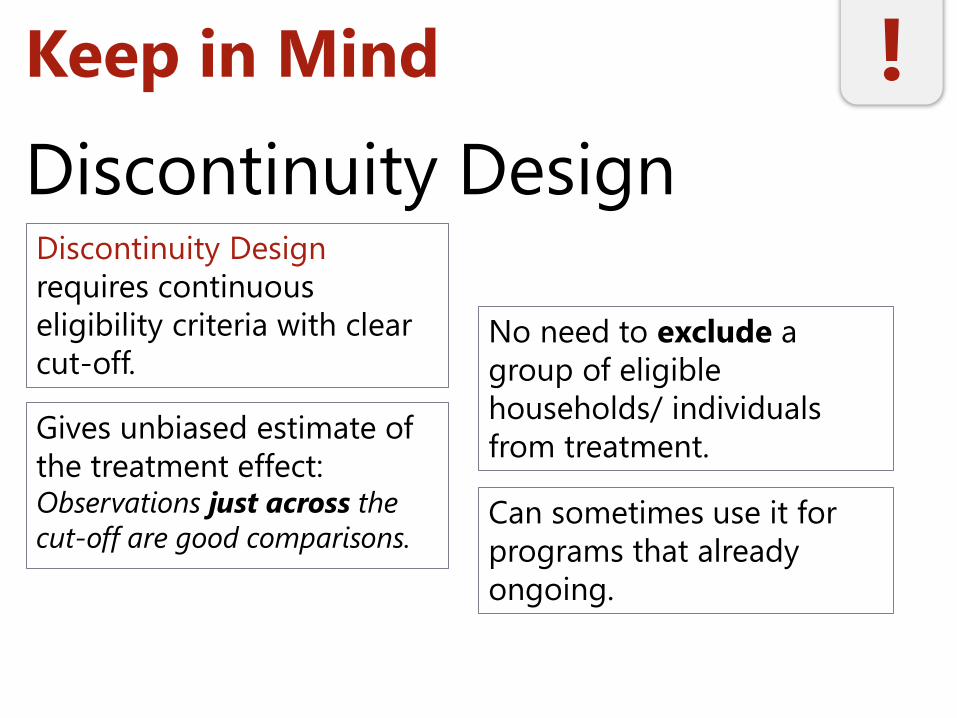
Keep in Mind
Discontinuity Design Discontinuity Design requires continuous eligibility criteria with clear cut-off.
Gives unbiased estimate of the treatment effect: Observations just across the cut-off are good comparisons.
No need to exclude a group of eligible households/ individuals from treatment.
Can sometimes use it for programs that already ongoing.
!

Keep in Mind
Discontinuity Design Discontinuity Design produces a local estimate: o Effect of the program
around the cut-off point/discontinuity.
o This is not always generalizable.
Power: o Need many observations around the cut-off point.
Avoid mistakes in the statistical model: Sometimes what looks like a discontinuity in the graph, is something else.
!

IE Methods Toolbox
Randomized Assignment
Discontinuity Design
Diff-in-Diff
Randomized Promotion
Difference-in-Differences
P-Score matching
Matching

Difference-in-differences (Diff-in-diff) Y=Wages P=Youth employment program
Diff-in-Diff: Impact=(Yt1-Yt0)-(Yc1-Yc0)
Enrolled Not Enrolled
After 0.74 0.81
Before 0.60 0.78
Difference +0.14 +0.03 0.11
- -
- =

Difference-in-differences (Diff-in-diff)
Diff-in-Diff: Impact=(Yt1-Yc1)-(Yt0-Yc0)
Y=School attendance P=Girls’ scholarship program
Enrolled Not Enrolled
After 0.74 0.81
Before 0.60 0.78
Difference
-0.07
-0.18
0.11
- -
-
=

Impact =(A-B)-(C-D)=(A-C)-(B-D) Sc
hool
Att
enda
nce
B=0.60
C=0.81
D=0.78
T=0 T=1 Time
Enrolled
Not enrolled
Impact=0.11 A=0.74
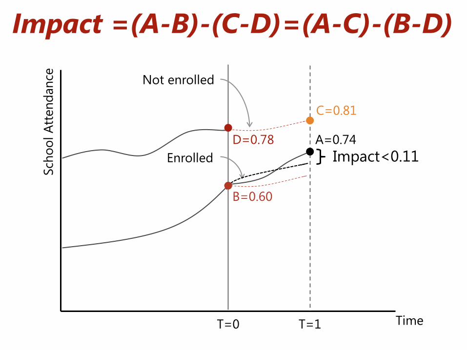
Impact =(A-B)-(C-D)=(A-C)-(B-D) Sc
hool
Att
enda
nce
Impact<0.11
B=0.60
A=0.74
C=0.81
D=0.78
T=0 T=1 Time
Enrolled
Not enrolled
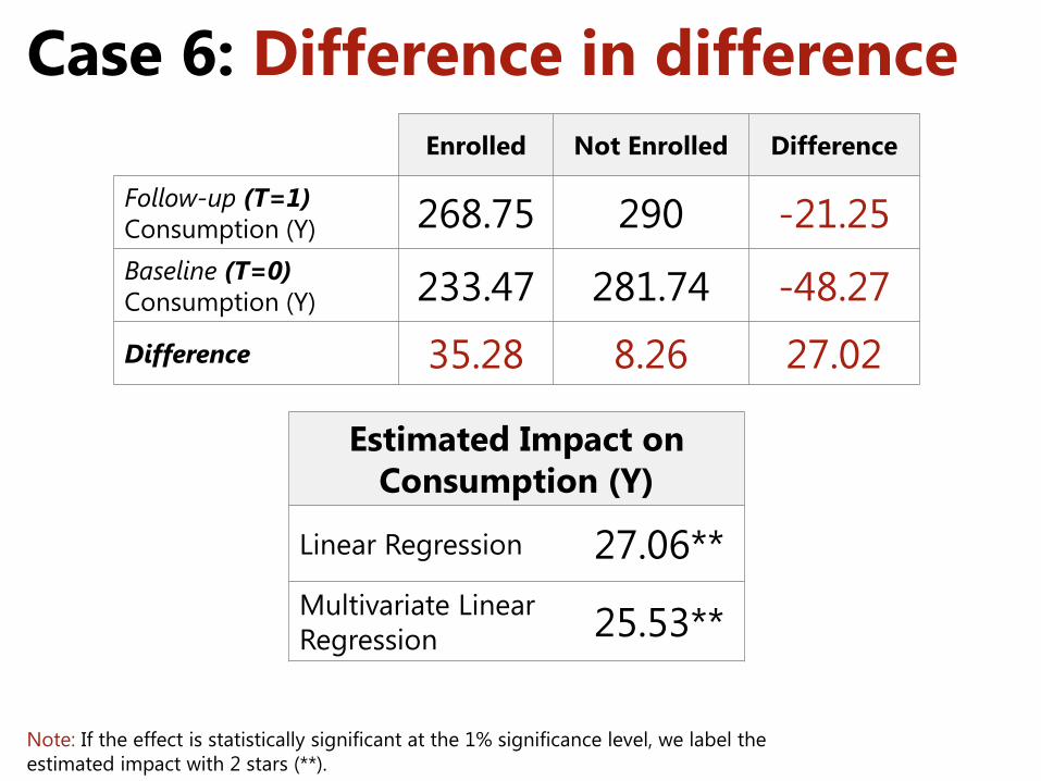
Case 6: Difference in difference Enrolled Not Enrolled Difference
Follow-up (T=1) Consumption (Y) 268.75 290 -21.25 Baseline (T=0) Consumption (Y) 233.47 281.74 -48.27 Difference 35.28 8.26 27.02
Estimated Impact on Consumption (Y)
Linear Regression 27.06** Multivariate Linear Regression 25.53**
Note: If the effect is statistically significant at the 1% significance level, we label the estimated impact with 2 stars (**).

Progresa Policy Recommendation?
Note: If the effect is statistically significant at the 1% significance level, we label the estimated impact with 2 stars (**).
Impact of Progresa on Consumption (Y)
Case 1: Before & After 34.28** Case 2: Enrolled & Not Enrolled -4.15 Case 3: Randomized Assignment 29.75** Case 4: Randomized Promotion 30.4** Case 5: Discontinuity Design 30.58** Case 6: Difference-in-Differences 25.53**

Keep in Mind
Difference-in-Differences Differences in Differences combines Enrolled & Not Enrolled with Before & After.
Slope: Generate counterfactual for change in outcome
Trends –slopes- are the same in treatments and comparisons (Fundamental assumption).
To test this, at least 3 observations in time are needed: o 2 observations before o 1 observation after.
!

IE Methods Toolbox
Randomized Assignment
Discontinuity Design
Diff-in-Diff
Randomized Promotion
Difference-in-Differences
P-Score matching
Matching
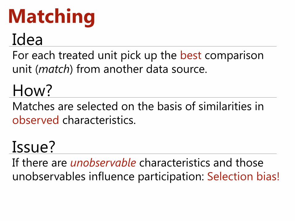
Matching
For each treated unit pick up the best comparison unit (match) from another data source.
Idea
Matches are selected on the basis of similarities in observed characteristics.
How?
If there are unobservable characteristics and those unobservables influence participation: Selection bias!
Issue?

Propensity-Score Matching (PSM) Comparison Group: non-participants with same observable characteristics as participants. o In practice, it is very hard. o There may be many important characteristics!
Match on the basis of the “propensity score”, Solution proposed by Rosenbaum and Rubin: o Compute everyone’s probability of participating, based
on their observable characteristics. o Choose matches that have the same probability of
participation as the treatments. o See appendix 2.
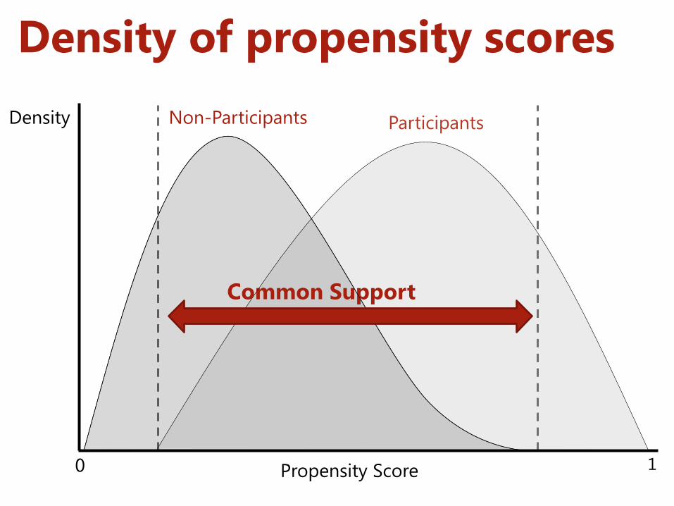
Density of propensity scores Density
Propensity Score 0 1
Participants Non-Participants
Common Support

Case 7: Progresa Matching (P-Score) Baseline Characteristics Estimated Coefficient
Probit Regression, Prob Enrolled=1
Head’s age (years) -0.022** Spouse’s age (years) -0.017** Head’s education (years) -0.059** Spouse’s education (years) -0.03** Head is female=1 -0.067 Indigenous=1 0.345** Number of household members 0.216** Dirt floor=1 0.676** Bathroom=1 -0.197** Hectares of Land -0.042** Distance to Hospital (km) 0.001* Constant 0.664**
Note: If the effect is statistically significant at the 1% significance level, we label the estimated impact with 2 stars (**).
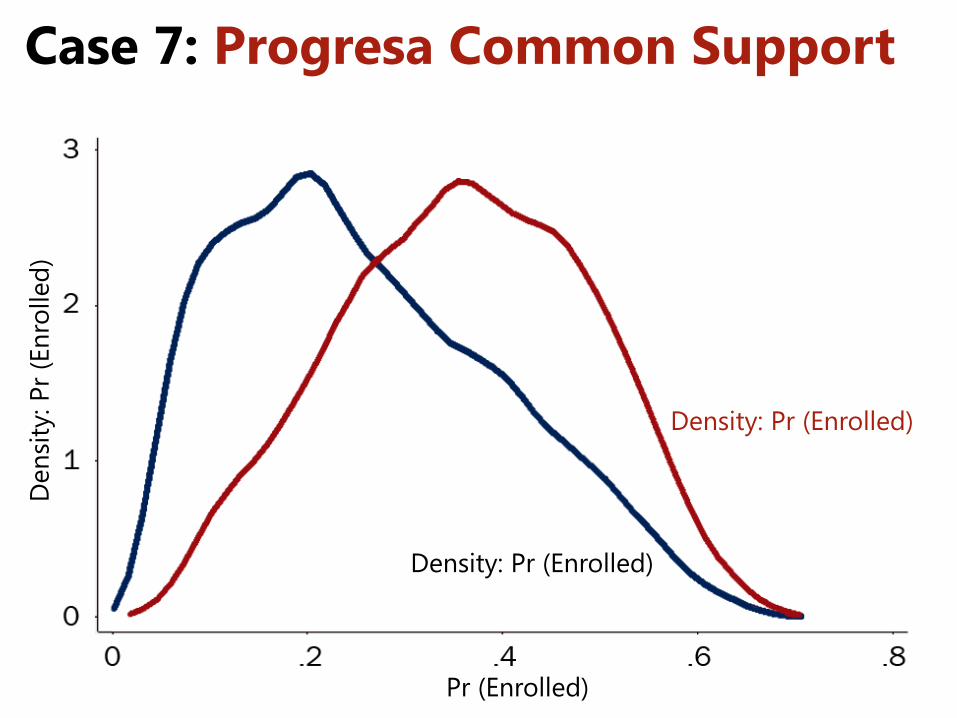
Case 7: Progresa Common Support
Pr (Enrolled)
Density: Pr (Enrolled)
Den
sity
: Pr (
Enro
lled)
Density: Pr (Enrolled)
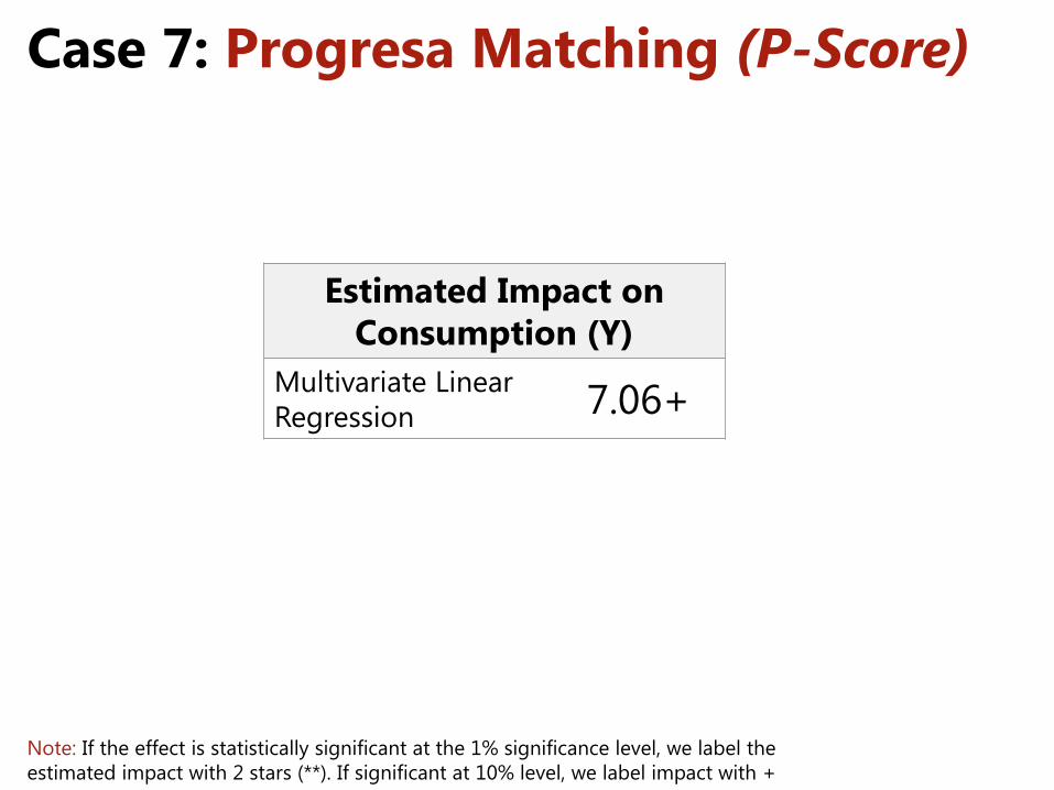
Case 7: Progresa Matching (P-Score)
Estimated Impact on Consumption (Y)
Multivariate Linear Regression 7.06+
Note: If the effect is statistically significant at the 1% significance level, we label the estimated impact with 2 stars (**). If significant at 10% level, we label impact with +

Keep in Mind
Matching Matching requires large samples and good quality data.
Matching at baseline can be very useful: o Know the assignment rule
and match based on it o combine with other
techniques (i.e. diff-in-diff)
Ex-post matching is risky: o If there is no baseline, be
careful! o matching on endogenous
ex-post variables gives bad results.
!

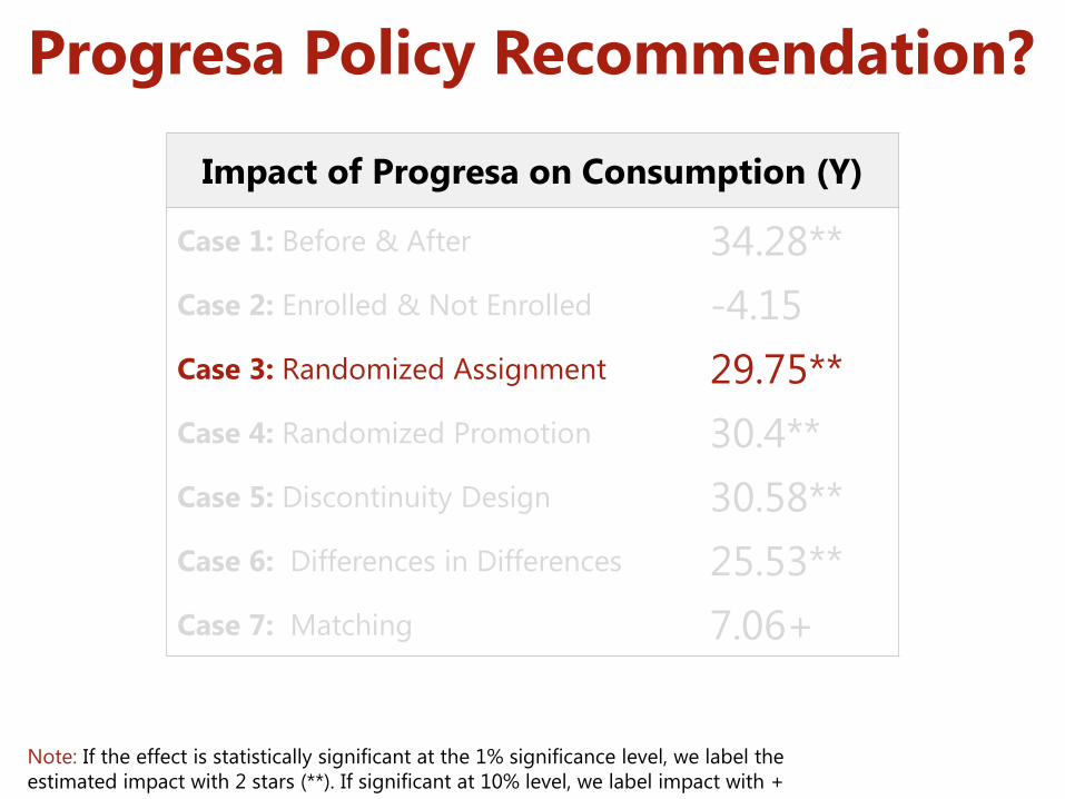
Progresa Policy Recommendation?
Note: If the effect is statistically significant at the 1% significance level, we label the estimated impact with 2 stars (**). If significant at 10% level, we label impact with +
Impact of Progresa on Consumption (Y)
Case 1: Before & After 34.28** Case 2: Enrolled & Not Enrolled -4.15 Case 3: Randomized Assignment 29.75** Case 4: Randomized Promotion 30.4** Case 5: Discontinuity Design 30.58** Case 6: Differences in Differences 25.53** Case 7: Matching 7.06+

IE Methods Toolbox
Randomized Assignment
Discontinuity Design
Diff-in-Diff
Randomized Promotion
Difference-in-Differences
P-Score matching
Matching
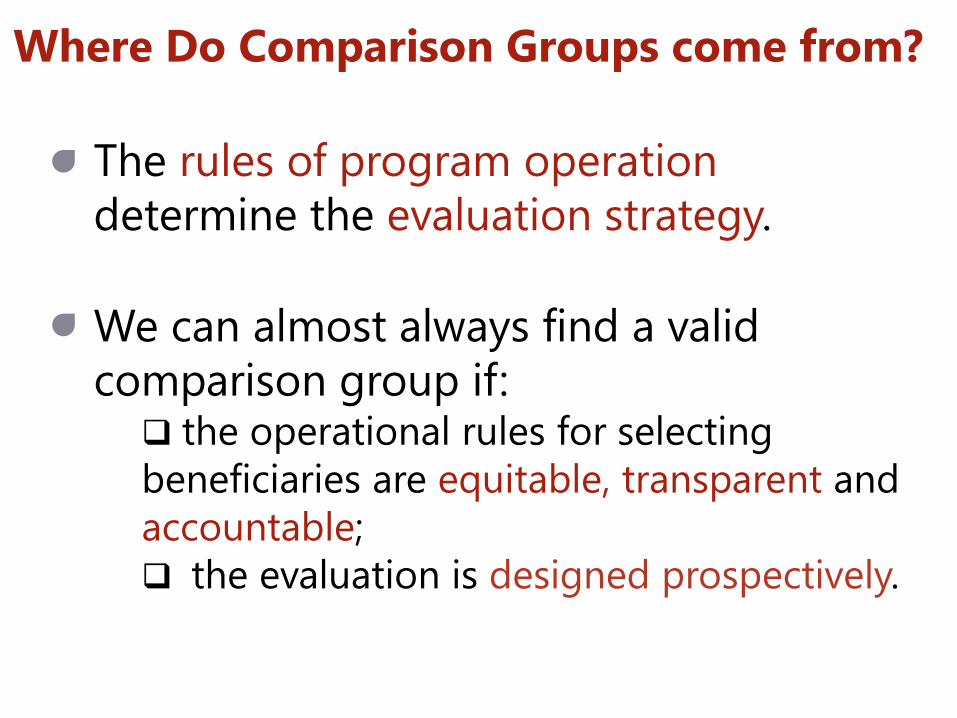
Where Do Comparison Groups come from?
The rules of program operation determine the evaluation strategy.
We can almost always find a valid comparison group if: the operational rules for selecting beneficiaries are equitable, transparent and accountable; the evaluation is designed prospectively.

Operational rules and prospective designs
Use opportunities to generate good comparison groups and ensure baseline data is collected.
3 questions to determine which method is appropriate for a given program
Money: Does the program have sufficient resources to achieve scale and reach full coverage of all eligible beneficiaries? Targeting Rules: Who is eligible for program benefits? Is the program targeted based on an eligibility cut-off or is it available to everyone? Timing: How are potential beneficiaries enrolled in the program – all at once or in phases over time?
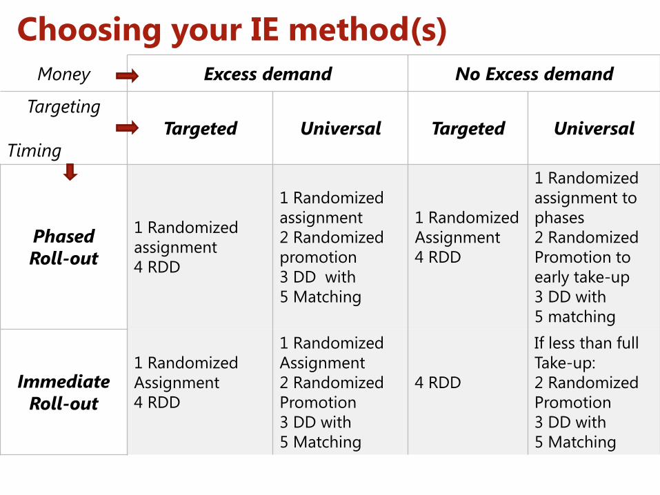
Choosing your IE method(s) Money Excess demand No Excess demand
Targeting
Timing Targeted Universal Targeted Universal
Phased Roll-out
1 Randomized assignment 4 RDD
1 Randomized assignment 2 Randomized promotion 3 DD with 5 Matching
1 Randomized Assignment 4 RDD
1 Randomized assignment to phases 2 Randomized Promotion to early take-up 3 DD with 5 matching
Immediate Roll-out
1 Randomized Assignment 4 RDD
1 Randomized Assignment 2 Randomized Promotion 3 DD with 5 Matching
4 RDD
If less than full Take-up: 2 Randomized Promotion 3 DD with 5 Matching
Remember
The objective of impact evaluation is to estimate the causal effect or impact of a program on outcomes of interest.

Remember
To estimate impact, we need to estimate the counterfactual. o what would have happened in the absence of
the program and o use comparison or control groups.

Remember
We have a toolbox with 5 methods to identify good comparison groups.

Remember
Choose the best evaluation method that is feasible in the program’s operational context.

Spanish Version & French Version
also available
www.worldbank.org/ieinpractice
Reference

Appendix 2 Steps in Propensity Score Matching
1. Representative & highly comparables survey of non-participants and participants.
2. Pool the two samples and estimated a logit (or probit) model of program participation.
3. Restrict samples to assure common support (important source of bias in observational studies)
4. For each participant find a sample of non-participants that have similar propensity scores
5. Compare the outcome indicators. The difference is the estimate of the gain due to the program for that observation.
6. Calculate the mean of these individual gains to obtain the average overall gain.