Measuring canopy loss and climatic thresholds from an ... · PRIMARY RESEARCH ARTICLE Measuring...

P R IMA R Y R E S E A R CH A R T I C L E

Measuring canopy loss and climatic thresholds from anextreme drought along a fivefold precipitation gradient acrossTexas

Amanda M. Schwantes1 | Jennifer J. Swenson1 | Mariano Gonz�alez-Roglich1,2 |

Daniel M. Johnson1,3 | Jean-Christophe Domec1,4 | Robert B. Jackson1,5

1Nicholas School of the Environment, Duke

University, Durham, NC, USA

2Conservation International, Arlington, VA,

USA

3Department of Forest, Rangeland, and Fire

Sciences, University of Idaho, Moscow, ID,

USA

4Bordeaux Sciences Agro, UMR INRA-ISPA

1391, Gradignan, France

5Department of Earth System Science,

Woods Institute for the Environment, and

Precourt Institute for Energy, Stanford

University, Stanford, CA, USA

Correspondence

Amanda M. Schwantes, Nicholas School of

the Environment, Duke University, Durham,

NC, USA.

Email: [email protected]

Funding information

National Aeronautics and Space

Administration, Grant/Award Number: Earth

and Space Science Fellowship

(NNX13AN86H); National Institute of Food

and Agriculture, Grant/Award Number:

2012-68002-19795

Abstract

Globally, trees are increasingly dying from extreme drought, a trend that is expected

to increase with climate change. Loss of trees has significant ecological, biophysical,

and biogeochemical consequences. In 2011, a record drought caused widespread

tree mortality in Texas. Using remotely sensed imagery, we quantified canopy loss

during and after the drought across the state at 30-m spatial resolution, from the

eastern pine/hardwood forests to the western shrublands, a region that includes the

boundaries of many species ranges. Canopy loss observations in ~200 multitemporal

fine-scale orthophotos (1-m) were used to train coarser Landsat imagery (30-m) to

create 30-m binary statewide canopy loss maps. We found that canopy loss

occurred across all major ecoregions of Texas, with an average loss of 9.5%. The

drought had the highest impact in post oak woodlands, pinyon-juniper shrublands

and Ashe juniper woodlands. Focusing on a 100-km by ~1,000-km transect spanning

the State’s fivefold east–west precipitation gradient (~1,500 to ~300 mm), we com-

pared spatially explicit 2011 climatic anomalies to our canopy loss maps. Much of

the canopy loss occurred in areas that passed specific climatic thresholds: warm sea-

son anomalies in mean temperature (+1.6°C) and vapor pressure deficit (VPD,

+0.66 kPa), annual percent deviation in precipitation (�38%), and 2011 difference

between precipitation and potential evapotranspiration (�1,206 mm). Although simi-

larly low precipitation occurred during the landmark 1950s drought, the VPD and

temperature anomalies observed in 2011 were even greater. Furthermore, future cli-

mate data under the representative concentration pathway 8.5 trajectory project

that average values will surpass the 2011 VPD anomaly during the 2070–2099 per-

iod and the temperature anomaly during the 2040–2099 period. Identifying vulnera-

ble ecological systems to drought stress and climate thresholds associated with

canopy loss will aid in predicting how forests will respond to a changing climate and

how ecological landscapes will change in the near term.

K E YWORD S

change detection, climate change, disturbance, extreme event, forest die-off, random forests,

tree mortality, vapor pressure deficit

Received: 4 December 2016 | Revised: 4 May 2017 | Accepted: 7 May 2017

DOI: 10.1111/gcb.13775

5120 | © 2017 John Wiley & Sons Ltd wileyonlinelibrary.com/journal/gcb Glob Change Biol. 2017;23:5120–5135.

http://orcid.org/0000-0002-7791-1078

http://orcid.org/0000-0002-7791-1078

http://orcid.org/0000-0002-7791-1078

http://wileyonlinelibrary.com/journal/GCB

1 | INTRODUCTION

As climate change progresses, droughts in many areas are expected

to increase in severity, duration, and frequency and, as a result, for-

ests will likely become more vulnerable to drought-induced tree

mortality (Allen, Breshears, & McDowell, 2015). Already, tree mortal-

ity events have been observed across the globe (Allen et al., 2010),

ranging from increases in background mortality rates (van Mantgem

et al., 2009) to regional die-offs (Breshears et al., 2005). As tempera-

ture extremes become more common under climate change, the like-

lihood of droughts occurring simultaneously with heatwaves is

increasing (AghaKouchak, Cheng, Mazdiyasni, & Farahmand, 2014).

These ‘hotter droughts’ can be particularly destructive to forests by

increasing respiration and, in consequence, the potential for carbon

starvation; increasing water stress due to rising atmospheric mois-

ture demand could also result in hydraulic failure (Allen et al., 2015).

Increased tree mortality will affect many critical factors, including

impacts to community composition (Mueller et al., 2005), food webs

(Carnicer et al., 2011), biophysics (Jackson et al., 2008; Rotenberg &

Yakir, 2010), carbon cycling (Ciais et al., 2005; Michaelian, Hogg,

Hall, & Arsenault, 2011), ecohydrology (Adams et al., 2012), stream

flow (Guardiola-Claramonte et al., 2011), and phenology (Ivits, Hor-

ion, Fensholt, & Cherlet, 2014). Forests provide important ecosystem

services; however, their fate under a changing climate with increased

drought and heatwaves is uncertain.

To improve forecasts of how forests will respond to climate

change, quantitative relationships between tree mortality and climate

are needed, even if these relationships are empirical (Adams et al.,

2013). Until the mechanisms surrounding tree death are well under-

stood and enough data exist to parameterize global vegetation mod-

els, empirical relationships may represent the most appropriate

avenue for forecasting tree mortality (Adams et al., 2013). Tree mor-

tality is often linked to reduced precipitation, increased temperature,

and associated increased vapor pressure deficit (VPD) (Allen et al.,

2015). VPD is defined as the difference between saturated vapor

pressure and actual vapor pressure and is largely dependent on tem-

perature. Other drought indices have been proposed that incorpo-

rate both precipitation and temperature. For example, the difference

between precipitation and potential evapotranspiration, P-PET,

accounts for both supply and atmospheric moisture demand (Rind,

Goldberg, Hansen, Rosenzweig, & Ruedy, 1990). A water deficit

occurs on the landscape when precipitation is less than potential

evapotranspiration and P-PET is negative. Furthermore, tree mortal-

ity often has a threshold response with climate (Clifford, Royer,

Cobb, Breshears, & Ford, 2013). Once a specific climatic anomaly is

surpassed, the likelihood of tree mortality increases substantially.

Many studies have linked mortality events to climatic anomalies.

These studies include tree-ring analysis to develop a forest drought

stress index in the southwest United States (Williams et al., 2013) as

well as field surveys in Amazonia and Borneo (Phillips et al., 2010)

and in Australia (Mitchell, O’Grady, Hayes, & Pinkard, 2014). How-

ever, fewer studies have examined relationships between remotely

sensed observations of tree mortality across climatic gradients. For

example, precipitation and VPD thresholds were related to pinyon

pine (Pinus edulis) mortality for a sub region of New Mexico (Clifford

et al., 2013), and climatic water deficit was linked to aspen (Populus

tremuloides) mortality in a part of Colorado (Anderegg et al., 2015).

Such studies focused on one natural system with only a couple of

dominant tree species. In this study, we examine remotely sensed

observations of tree mortality across a much larger climatic gradient

from humid to semiarid regions. Through remote sensing, climate

can be linked to continuous spatially explicit estimates of tree mor-

tality across large areas, closer to the extent of regional vegetation

models.

Remote sensing approaches tailored specifically for drought-

induced tree mortality that can span large areas at a fine resolution

are also needed. Tree mortality caused by drought is often an irregu-

lar process by which some individuals die but neighboring trees

remain alive. Dead trees scattered among many live trees are more

difficult to quantify using remote sensing approaches compared to

disturbances that kill entire stands (McDowell et al., 2015). At coar-

ser scales, pixels are often ‘mixed’, containing multiple cover types

(i.e., canopy loss and live canopy) and there may be excess zero pix-

els (i.e., homogenous live canopy cover), if low-levels of mortality

occur. Many remote sensing techniques have been proposed to

quantify drought-induced tree mortality, including spectral mixture

analysis (Huang & Anderegg, 2012), zero-inflated models (Schwantes,

Swenson, & Jackson, 2016), and time-series of spectral indices

(Vogelmann, Tolk, & Zhu, 2009; Meddens, Hicke, Vierling, & Hudak,

2013). However, these studies were designed for mapping mortality

in only one natural system with a few dominant species. Other stud-

ies have proposed techniques that work across systems using

Moderate Resolution Imaging Spectroradiometer (MODIS), such as

the MODIS global disturbance index (Mildrexler, Zhao, & Running,

2009) and the ForWarn system (Norman, Koch, & Hargrove, 2016).

However, the spatial resolution of these products ranges from

250 m to 1 km, which is too coarse to capture local-scale distur-

bances (McDowell et al., 2015). Alternatively, the 30-m resolution of

Landsat imagery is a more appropriate scale to detect forest cover

changes (Cohen & Goward, 2004). In this study, we implement a

remote sensing approach that (i) maps canopy loss across diverse

ecoregions at regional scales and (ii) accommodates excess zeros and

mixed pixels, inherent to disturbances like drought-induced tree mor-

tality.

Texas was advantageous for studying drought-induced tree mor-

tality because it was the location of an extreme drought and heat

wave in 2011 and it spans a large climatic gradient from humid to

semiarid regions. Using statewide averages of Palmer Drought Sever-

ity Index (PDSI) data from 1895 to 2011, Hoerling et al. (2013)

found that the 2011 drought reached a record statewide minimum

PDSI of �7.93. The 2011 drought was also the driest 12-month per-

iod, October 2010 to September 2011, on record (Hoerling et al.,

2013). Furthermore, due to low atmospheric moisture and high tem-

peratures, the 2011 drought was also associated with a record high

VPD (Williams et al., 2014). Although it is challenging to definitively

link episodic climatic events to climate change, models indicate that

SCHWANTES ET AL. | 5121

abnormally high summer temperatures in Texas are increasing in like-

lihood (Rupp et al., 2015). Furthermore, in the southwestern United

States, temperature and VPD are projected to increase in the future

(Williams et al., 2014). Texas has over 200 ecological plant commu-

nity types dominated by woody species (Elliott et al., 2014), span-

ning a broad range of annual precipitation regimes from humid to

semiarid. As such, Texas contains the most arid edge of many spe-

cies’ ranges (e.g., the eastern hardwoods). These trailing range edges

often see heightened drought-induced tree mortality (Jump, M�aty�as,

& Pe~nuelas, 2009).

In this study, we identify empirical relationships between climate

and canopy loss observed during and after the drought and deter-

mine if, and when, the 2011 climatic anomalies are projected to be

crossed in the future. To detect canopy loss from the 2011 drought

across Texas, we first created a multitemporal training dataset by

classifying 194 fine-scale 1-m orthophoto sets (Schwantes et al.,

2016). We then used random forests models to relate the canopy

loss observed in the 1-m orthophoto classifications to 30-m Landsat

imagery to estimate drought impact across the state of Texas. These

coarse-scale regional maps were used to identify ecological systems

most impacted by the drought. We also identified threshold relation-

ships between climate and spatial patterns of canopy loss across the

fivefold precipitation gradient spanning humid to semiarid regions.

Lastly, we examined whether the 2011 climate anomalies would

likely be surpassed in the future using downscaled projected climate

data, under representative concentration pathway, RCP, 4.5 and 8.5

trajectories.

2 | MATERIALS AND METHODS

2.1 | Study area

The state of Texas was selected because (i) it was the center of a

major drought and tree mortality event in 2011, (ii) its natural pre-

cipitation gradient was large for areas dominated by tree cover,

extending from mean annual precipitation (MAP) of ~1,500 mm in

the east to ~300 mm in the west, and (iii) it included the edges of

many species’ ranges (e.g., eastern hardwoods such as Quercus stel-

lata and many western shrubland species like Juniperus ashei). The

12 U.S. EPA level III ecoregions in the state of Texas followed the

east–west precipitation gradient, transitioning from dense closed-

canopy forests to the open-canopy savannas to the western shrub-

lands (Table 1). We excluded the high plains in this study, because

the area was dominated by grasslands, with little or no woody plant

cover. We divided our study area into six zones for purposes of

modeling by combining the 11 ecoregions into zones based on

similar species and climate: (i) Pineywoods, (ii) Oakwoods/Blackland

Prairies, (iii) Rolling Plains, (iv) Edwards Plateau, (v) South Texas, and

(vi) Trans Pecos (Figure 1, Table 1). A decrease in precipitation and

an increase in mean temperature compared to historical averages

were observed during the 2011 drought across all six modeling

zones (Table 1; PRISM Climate Group, 2015). Moreover, precipita-

tion decreased by more than half of the historical average for the

Trans Pecos and Edwards Plateau.

2.2 | Creating training and testing data:classification and field validation of 1-m canopy lossmaps

Following Schwantes et al. (2016), we created a training and testing

dataset of fine-scale canopy loss maps, from supervised classifica-

tions of stacks of predrought (2010) and postdrought (2012)

orthophotos from the National Agriculture Imagery Program (NAIP)

(US Department of Agriculture, 2014). The 1-m orthophotos (four

bands: red, green, blue, near-infrared, NIR) were flown during the

growing season, were already orthorectified to true ground, errors

within 6 m, and were tiled based on quarter quads, each ~41 km2.

We randomly selected 186 NAIP quarter quads using a blocked ran-

dom sample, where blocks were the Landsat footprints (each

~23,000 km2), excluding areas of overlapping Landsat scenes. The

number of NAIP quarter quads chosen per Landsat footprint was

weighted by the forest-area proportion in the Landsat footprint. We

TABLE 1 Climate data (historical averages and 2011 values) for the six modeling zones

Modeling zone Level III ecoregions (U.S. EPA)

Spatial mean of annualprecipitation (mm)

Spatial mean ofwarm season mean temp (˚C)

Hist. mean � SDa 2011 mean Hist. mean � SDa 2011 mean

1. Pineywoods • South Central Plains 1222 � 228 826 25.9 � 0.7 28.1

2. Oakwoods & Blackland Prairies • Texas Blackland Prairies

• East Central Texas Plains

948 � 195 608 26.6 � 0.7 28.6

3. Rolling Plains • Southwestern Tablelands

• Central Great Plains

• Cross Timbers

646 � 124 380 25.5 � 0.8 28.0

4. Trans Pecos • Arizona/New Mexico Mountains

• Chihuahuan Deserts

317 � 100 110 25.0 � 0.7 27.1

5. Edwards Plateau • Edwards Plateau 614 � 150 295 25.7 � 0.7 27.7

6. South Texas & Gulf Coast • Southern Texas Plains

• Western Gulf Coastal Plain

767 � 172 384 27.9 � 0.6 29.3

aThe historical mean and standard deviation as calculated for years 1950 to 2005, using PRISM data (PRISM Climate Group, 2015).

5122 | SCHWANTES ET AL.

selected an additional eight orthophotos nonrandomly based on

access to public land, for the purpose of field validation; field access

was limited in Texas.

For validation, we compared observations of canopy loss in the

1-m orthophoto classifications to measurements of dead and live

crowns taken on the ground, following Schwantes et al. (2016). From

July to Sept 2013 and during July 2014, we measured dead and live

crowns in 13 sites (Figure 1), with 3–7 plots per site (Table S1), for a

total of 67 plots. For each plot, we measured dead and live crowns

(to the nearest 0.1-m) along four 25-m transects running from the

randomized plot center to the plot edge following the four cardinal

directions. All woody species >1-m in height were counted that

intersected the transect. Rules for assigning the health status to each

individual tree (e.g., dead, live, dead prior to drought) were outlined

in Table S2. Canopy cover loss measurements of the uppermost

layer of canopy, from each of the four transects, were summed for

each plot, and compared to the total canopy loss observed in the

orthophoto classifications, as estimated within a 25-m radius circular

buffer from plot center. Further details on classification and valida-

tion of the orthophotos are described in Schwantes et al. (2016) and

the supporting information.

2.3 | Scaling up to regional estimates using randomforests: 30-m binary canopy loss map

To focus our analysis within forested regions and avoid misclassifica-

tions associated with fires and clearing, we excluded areas that were

nonforest, burned, or cleared. We created a binary forest cover mask

by including only ecological systems dominated by tree species

(Elliott et al., 2014). Using data from the Monitoring Trends in Burn

Severity project (USDA Forest Service/U.S. Geological Survey, 2014),

we also excluded all areas that were burned from May 2009 to Oct

2014. Lastly, through visual inspection we used a band difference

between postdrought and predrought tassel cap brightness bands

(Crist, 1985; Baig, Zhang, Shuai, & Tong, 2014) of 0.1 to remove

trees that were cleared in the Pineywoods and Oakwoods/Blackland

Prairies and 0.2 for the four remaining western modeling zones.

Atmospherically corrected imagery from the Landsat surface

reflectance product (Masek et al., 2006) was acquired from May to

Oct with a preference for late summer images. Predrought images

were either taken in 2009 or 2010 from the Landsat 5 TM archive.

Landsat 5 TM became nonoperational Nov 2011, and Landsat 8 OLI,

launched Feb 2013; therefore postdrought images were from the

Landsat 8 OLI archive, 2–3 years after the drought (2013 or 2014;

see Table S3 for acquisition dates). We manually co-registered NAIP

images that showed poor alignment with Landsat scenes to achieve

an RMSE <0.5 of a 30-m Landsat pixel.

To scale up from the 1-m orthophoto classifications to the 30-m

Landsat imagery, we used random forests models (Breiman, 2001;

Liaw & Wiener, 2002) in classification mode to create 30-m binary

maps (loss or no loss) across Texas. Using a separate model for each

of the six modeling zones, we employed random forests, a machine

learning algorithm that created an ensemble of decision trees. Each

decision tree was grown using a sample of the data and a subset of

the explanatory variables. The nodes on each decision tree were cre-

ated by splitting the explanatory variables in a way that created the

most homogenous groups, until a minimum/terminal node size was

reached. Bootstrap samples were taken with replacement to

F IGURE 1 Modeling zones of Texascharacterized as temperate deciduousforest, grassland, and desert biomes. TheHigh Plains, nonforested, burned, andcleared areas were excluded from theanalysis. We estimated canopy loss acrossthree scales: field estimates of canopy loss(67 plots) were used to validate the fine-scale canopy loss maps derived from 1-morthophotos (n = 194 at ~41 km2 each),which were used to scale up to Landsat(46 footprints covering Texas,~600,000 km2) [Colour figure can beviewed at wileyonlinelibrary.com]


build each decision tree; data withheld were used to compute the

out-of-bag (OOB) error rate (Breiman, 2001). We did not find that

our models were sensitive to parameterization; therefore, we used

the following: 1001 decision trees, a node size of 1, and the number

of variables used to build each decision tree equal to the square root

of the total number of variables. By overlaying a grid at the spatial

resolution of Landsat (30-m) onto the 1-m orthophoto classifications,

we extracted proportion canopy loss for each 30-m grid cell and

created a binary response variable for the random forests models: (i)

pixels with zero canopy loss (no loss pixels with homogenous live

canopy) and (ii) pixels with greater than 25% canopy loss (loss pix-

els). The explanatory variables for the random forests models were

percent tree cover from the National Land Cover Databases (NLCD)

(Homer et al., 2015) and 13 vegetation indices derived from Landsat

(Table 2) for both pre and postdrought images. For variable selec-

tion, we created parsimonious models by removing variables that

were highly correlated to greater than |0.95|. The final variables

selected for each random forests model can be found in Table S4.

Much of the landscape experienced no mortality; thus, the

canopy loss dataset contained many more pixels with zero canopy

loss compared to pixels with greater than 25% canopy loss, and

therefore, to improve the random forests model fits we made the

following modifications. Firstly, we sampled each class equally for

each decision tree in the random forests. Secondly, using random

forests model outputs of the probability of a pixel’s class member-

ship, we tuned the models with receiver operating characteristic

(ROC) curves (Sing, Sander, Beerenwinkel, & Lengauer, 2005). To

determine the class of each pixel (e.g., canopy loss vs. no loss), we

balanced true positive rate (TPR, accurately predicting a loss pixel

when a loss pixel occurred) and true negative rate (TNR, accurately

predicting a no loss pixel when no loss pixel occurred). Finally, to

remove the influence of slight atmospheric differences between

Landsat scenes, the random forests model was first run using all data

within the modeling zone. Then, unique probability thresholds were

chosen using the ROC analysis based on groups of Landsat foot-

prints. Groups were chosen to match rows with similar acquisition

dates or for individual Landsat scenes that had unique acquisition

dates. The cutoff values used to define a loss pixel from a no loss

pixel can be found in Table S5 and a more detailed explanation of

the ROC analysis can be found in the supporting information.

Not every pixel contained 100% canopy loss, and therefore to

estimate the overall percent canopy loss, we multiplied the propor-

tion of impacted 30-m pixels by the average canopy loss within each

of the impacted pixels, as estimated using the 1-m orthophoto classi-

fications for each modeling zone. We used the same procedure to

compute overall relative canopy loss, defined as canopy loss divided

by the live predrought canopy cover. In this way, we could more

precisely determine the percent of forest impacted by the drought.

To test model performance, we used spatially independent testing

data, which provided a better estimate of the true mapping accuracy

(Gonz�alez-Roglich & Swenson, 2016; Schwantes et al., 2016), by

conducting leave-one-out cross validation for each orthophoto, inde-

pendently for each of the six modeling zones (see supporting infor-

mation for a complete description). As is the case for most remote

sensing studies, we were only mapping aerial cover, defined as the

uppermost layer of canopy (Fehmi, 2010); we were not mapping

overlapping canopy cover. For example, if the overstory died and

the midstory or understory remained alive, we would still consider

this canopy loss. Moreover, analysis relying on remotely sensed ima-

gery detects changes in canopy; therefore, we used the terms

canopy loss and live canopy instead of dead and live trees. Image

processing for the coarse-scale maps was completed in ENVI/IDL

5.0, ArcMap 10.3.1, Python 2.7.8, and R v. 3.1.3 (R Core Team,

2015).

2.4 | Defining relationships between spatialpatterns of canopy loss and climate

To examine how climate drove the spatial patterning of canopy loss

across a landscape, we used 4-km spatially interpolated climate data

from PRISM (PRISM Climate Group, 2015). For each 4-km cell, we

first calculated the relative canopy loss, defined as the number of

30-m drought-impacted pixels divided by the number of forest cover

pixels. We then examined how four climate variables: annual precipi-

tation, warm season (May–Sept) mean temperature, warm season

VPD, and annual 2011 P-PET controlled mortality patterns across an

east–west transect that was 100 km wide by ~1,000 km in length. In

selecting the transect, we chose the widest horizontal swath across

Texas that encompassed the greatest amount of ecosystem diversity.

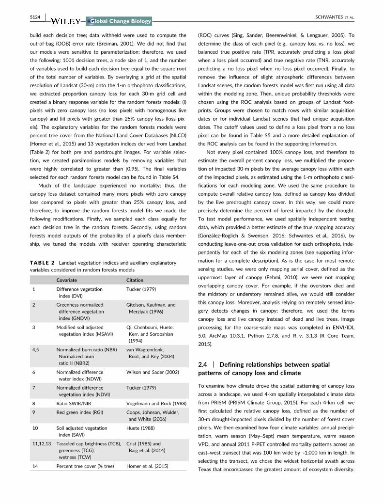
TABLE 2 Landsat vegetation indices and auxiliary explanatoryvariables considered in random forests models

Covariate Citation

1 Difference vegetation

index (DVI)

Tucker (1979)

2 Greenness normalized

difference vegetation

index (GNDVI)

Gitelson, Kaufman, and

Merzlyak (1996)

3 Modified soil adjusted

vegetation index (MSAVI)

Qi, Chehbouni, Huete,

Kerr, and Sorooshian

(1994)

4,5 Normalized burn ratio (NBR)

Normalized burn

ratio II (NBR2)

van Wagtendonk,

Root, and Key (2004)

6 Normalized difference

water index (NDWI)

Wilson and Sader (2002)

7 Normalized difference

vegetation index (NDVI)

Tucker (1979)

8 Ratio SWIR/NIR Vogelmann and Rock (1988)

9 Red green index (RGI) Coops, Johnson, Wulder,

and White (2006)

10 Soil adjusted vegetation

index (SAVI)

Huete (1988)

11,12,13 Tasseled cap brightness (TCB),

greenness (TCG),

wetness (TCW)

Crist (1985) and

Baig et al. (2014)

14 Percent tree cover (% tree) Homer et al. (2015)


As the transect spans a precipitation gradient, we calculated percent

deviations from historical values for precipitation; however, for tem-

perature and VPD we calculated anomalies, and for P-PET we used

the 2011 value. The analysis was conducted on a sample of 20% of

the 4-km pixels within the transect, excluding adjacent pixels with a

minimum distance between cell centers of <8 km. We also only

included pixels with >50% forested area to focus the analysis in pre-

dominantly forested regions. Precipitation and mean temperature

were directly acquired (PRISM Climate Group, 2015), and daily VPD

was calculated using mean temperature and dew point temperature

following Daly, Smith, and Olson (2015). PET was acquired from

GRIDMET, a 4-km gridded climate dataset, where PET was calcu-

lated using Penman-Monteith (Abatzoglou, 2013).

We identified climatic thresholds that when surpassed were

associated with greater canopy loss, based on the first split in

regression trees (Therneau, Atkinson, & Ripley, 2015). In this case,

the numeric response variable was relative canopy loss within a 4-

km pixel and the continuous explanatory variable was percent devia-

tion or anomaly from normal climate. For each climate variable, the

regression tree selected a breakpoint along the continuous climate

variable that created the most homogenous response group (De’ath

& Fabricius, 2000). In this way, climatic conditions associated with

large amounts of canopy loss were differentiated from climates asso-

ciated with little canopy loss. The breakpoint between these two

groups was considered the climatic threshold that when crossed led

to enhanced mortality. These climatic thresholds were identified

across space; therefore, to further validate whether these thresholds

could also hold true through time, we examined past climate from

1950 to 2015, using data from PRISM (PRISM Climate Group,

2015); however, PET data were only available from 1979 onwards

(Abatzoglou, 2013).

2.5 | Projecting whether 2011 climate anomalieswere likely to be crossed in the future

We determined whether the climate thresholds associated with

canopy loss in 2011 were likely to be crossed in the future. Firstly,

we acquired 4-km projected climate data, where statistical downscal-

ing had been performed using the multivariate adapted constructed

analogs (MACA) approach (Abatzoglou & Brown, 2012). Precipitation,

temperature, and PET were acquired directly (Abatzoglou & Brown,

2012), whereas daily VPD was computed using mean temperature

and specific humidity (Ross & Elliot, 1996). We examined the mean,

standard deviation, and range of 20 global climate models (GCMs),

using Coupled Model Intercomparison Project Phase 5 (CMIP5)

results, under the Representative Concentration Pathway (RCP) 4.5

and 8.5 trajectories from 2006 to 2099 (Abatzoglou & Brown,

2012). Secondly to calculate historical values used to compute the

anomalies from current climate, we used historical PRISM data

(1950–2005); however, for calculating the historical values used to

compute anomalies for future climate, we used historical projected

MACA data (1950–2005). We only considered pixels with >50%

forested area. Also, to further characterize the variability between

the models, we estimated the percent of times that these climatic

thresholds would be crossed over the latter half of the 21st century

(2050–2099) across the 20 GCMs, creating spatially explicit maps for

the state of Texas. For example, if 50% of the GCMs predicted that

a threshold crossing would occur for 50% of the years from 2050 to

2099, then this would be represented by an average 25% times

crossed.

2.6 | Identifying ecological systems most impactedby the 2011 drought

We determined which communities were most influenced by the

2011 drought through an overlay of our canopy loss maps and an

ecological systems layer map (Elliott et al., 2014; Comer et al.,

2003). We only considered ecological systems dominated by tree

species, 231 systems, and then we further only included geographi-

cally dominant systems that covered at least 200 km2, for a total of

94 systems. Of these 94 dominant systems, we present the top 10

most and least impacted, where the most impacted systems had the

largest relative canopy loss defined as drought-impacted area divided

by total area. The full analysis for all 231 tree-dominant systems can

be found in Table S6.

3 | RESULTS

Ground estimates of canopy loss and postdrought live canopy cover

were both highly correlated with the same attributes observed in

the orthophoto classifications (R2 = .82, RMSE = 4.7% for canopy

loss; R2 = .89 and RMSE = 11% for live canopy) (Figure 2). Overesti-

mation of canopy cover loss in the orthophotos happened occasion-

ally when trees lost most of their foliage and thus appeared dead in

the orthophotos. Underestimates of tree cover loss occurred on

occasion when dead trees were misclassified as alive, due to the

presence of either dense understory shrubs or grass under the dead

canopy, or extensive vines within the dead canopy.

In quantifying statewide 30-m binary canopy loss using random

forests models, error rates and the covariates found to be the most

important in predicting canopy loss were unique to each modeling

zone. The normalized burn ratio and tassel cap brightness (TCB)

indices were found to be the most important to modeling canopy

loss in the Pineywoods region, whereas TCB, tassel cap wetness,

and the difference vegetation index were the best predictors for the

Trans Pecos and Edwards Plateau (Table S4). The out-of-bag (OOB)

estimates of accuracy (ranging from 86% to 93%) were higher com-

pared to the spatially independent estimates (ranging from 79% to

90%) (Table 3), likely because the latter were tested using spatially

independent data. The spatially independent accuracy metric also

reflects that the data had excess zeros, and as such the models

tended to predict the common (no loss) pixels well (TNR), but the

rarer class (loss pixels) less well (TPR). The model with the highest

error was for the South Texas & Gulf Coast modeling zone

(Table 3).


Overall, 61,000 km2 of forested area was impacted by the

drought as defined by having >25% canopy loss per pixel (Figure 3,

Table 4). Within forested pixels across the state, the drought caused

an average 9.5% canopy loss and 15% relative canopy loss, defined

as canopy cover loss divided by predrought live canopy cover

(Table 4). Relative canopy loss was a more useful comparison metric

considering that average predrought percent live canopy ranged

from 21% in the Trans Pecos to 85% in the Pineywoods according

to the orthophoto classifications. The Pineywoods region was the

least impacted in terms of canopy loss and relative canopy loss. The

other five western modeling zones were severely impacted by the

drought when considering relative canopy loss.

Spatial patterns of canopy loss in Texas exhibited threshold

responses with warm season VPD, warm season temperature, annual

precipitation, and 2011 annual P-PET. When a climatic threshold

was surpassed, more tree mortality occurred. A threshold response

was apparent, where 4-km pixels had greater canopy loss with either

a VPD anomaly greater than 0.66 kPa, a temperature anomaly

greater than 1.6°C, a percent deviation in precipitation less than

�38%, or a 2011 P-PET water deficit less than �1,206 mm (Fig-

ure 4).

To test whether the climatic thresholds we identified for 2011

occurred in the past, we used PRISM data from 1950 to 2015. The

temperature threshold was only crossed twice, during 1998 and

2011 (Figure 5), whereas the VPD anomaly was only surpassed once,

during the 2011 drought. The precipitation threshold was crossed

twice (1950s and 2011) over the historical climate period. Precipita-

tion levels in 2011 were similar to the 1950s drought; however, the

2011 drought was uniquely characterized by higher temperatures

and VPDs.

The temperature threshold was projected to be surpassed on

average for the two time periods: 2040–2069 and 2070–2099 (black

diamonds in Figure 5), when considering an ensemble average across

20 GCMs, under RCP 4.5 and 8.5. However, the VPD anomaly and

the 2011 P-PET water deficit were both projected to be surpassed

on average only for the 2070–2099 period under the RCP 8.5 sce-

nario. Conversely, the future precipitation projection ensemble mean

did not project any crossings of these precipitation thresholds; how-

ever, the ensemble range and standard deviation did cross the

threshold in the future.

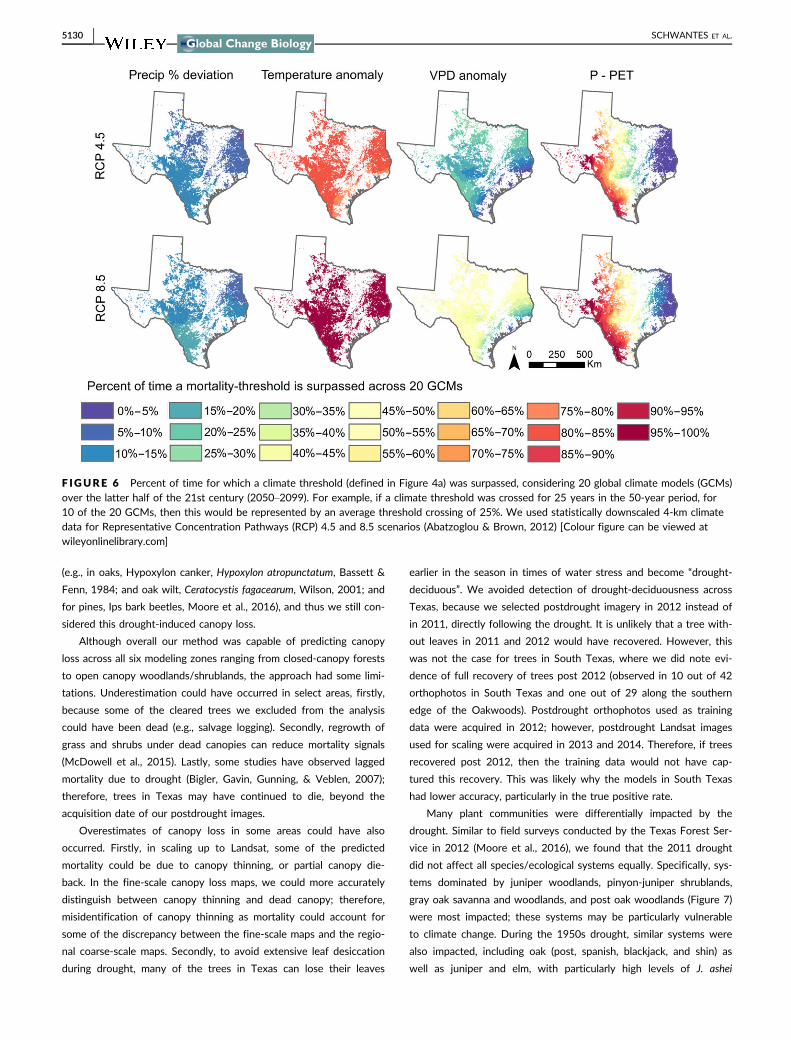
The proportion of times and models for which a threshold was pro-

jected to be crossed varied across space and was unique to each cli-

mate variable, when considering 20 GCMs and a 50-year time-period,

2050–2099 (Figure 6). Although, the ensemble mean for precipitation

was never projected to cross the precipitation threshold in the future,

for portions of the landscape, precipitation thresholds were crossed

4%–16% (RCP 4.5) and 6%–20% (RCP 8.5) of the time for the latter

half of the 21st century and across 20 GCMs. Thresholds were crossed

more often for VPD ranging from 0% to 28% (RCP 4.5) and 0% to 62%

(RCP 8.5) as well as for temperature ranging from 75% to 86% (RCP

4.5) and 96% to 98% (RCP 8.5) (Figure 6). P-PET threshold crossings

ranged from 0% to 100% for both RCP 4.5 and 8.5 scenarios. The pre-

cipitation thresholds were projected to be crossed more frequently for

Central and South Texas, for both RCP 4.5 and 8.5, and the southern

edge of East Texas (Pineywoods) for RCP 8.5. For VPD under both

F IGURE 2 Field validation: canopy lossand live canopy cover measured usingground transects (2013–2014) comparedto canopy loss and live canopy coverobserved in the 1-m orthophotoclassifications (imagery from 2010 and2012)

TABLE 3 Accuracy of random forests models in distinguishingpixels of canopy loss (>25%) from pixels of no (0%) canopy loss

Modeling zone

Spatially independent Final model (OOB)

%Accuracy

%TPR

%TNR

%Accuracy

%TPR

%TNR

Pineywoods 90 80 90 91 90 91

Oakwoods &

Blackland Prairie

83 61 83 88 87 88

Rolling Plains 79 53 80 86 87 86

Trans Pecos 83 68 83 93 90 93

Edwards Plateau 84 81 85 91 91 91

South Texas &

Gulf Coast

79 30 81 92 91 92

TPR, true positive rate (accurately predicting a loss pixel when a loss

pixel occurred); TNR, true negative rate (accurately predicting a no loss

pixel when a no loss pixel occurred).


scenarios, and for temperature under RCP 4.5, thresholds were less

likely to be crossed near the gulf coast; however, for RCP 8.5, the tem-

perature threshold was crossed almost uninterruptedly for most of the

region (Figure 6).

For the 94 ecological systems where trees were dominant and cov-

ered >200 km2 in area, we present the top most and least impacted

systems. Table S6 contains drought impacts for all 231 ecological sys-

tems dominated by tree species. The systems most negatively affected

by the 2011 drought (Figure 7) were the pinyon-juniper (Pinus cem-

broides, Juniperus deppeana, J. pinchotii, and J. flaccida) and oak systems

(Quercus grisea, Q. emoryi, Q. hypoleucoides, Q. arizonica, Q. rugose, and

Q. mohriana) of the Trans Pecos, the post oak (Q. stellata) woodlands

of the Llano uplift, and the juniper woodlands (J. ashei, J. virginiana, J.

monosperma and J. pinchotii) of the Edwards Plateau (Moir, 1982;

Elliott et al., 2014). Furthermore, systems on sandy sites (e.g., sandy

mesquite evergreen woodlands and sandy shinnery shrublands)

tended to have more canopy loss. Alternatively, systems in riparian

and mesic areas as well as managed systems were less impacted.

Lastly, communities dominated by the invasive Chinese Tallow (Triad-

ica sebifera L.), had some of the lowest canopy loss.

4 | DISCUSSION

We mapped drought-induced canopy loss using a consistent

method across a fivefold precipitation gradient that spanned

humid to semiarid regions. We took advantage of open-source

remotely sensed imagery at two spatial scales and new machine

TABLE 4 Summary of percent forest cover lost and impacted area by modeling zone

Modeling zoneEstimated areaimpacted (km2)

Avg. % canopyloss in loss pixelsa

Avg. relative % canopyloss in loss pixelsb

Overall avg. %canopy lossc

Overall avg. relative% canopy loss

Pineywoods 8,842 35 40 6.8 7.8

Oakwoods & Blackland Prairie 8,818 36 43 9.8 12

Rolling Plains 15,760 36 60 9.9 16

Trans Pecos 3,865 42 73 7.9 14

Edwards Plateau 11,522 39 65 8.8 15

South Texas & Gulf Coast 12,157 46 68 10 16

Total 60,969 41 63 9.5 15

a,bThe average percent canopy loss (col 3) and relative percent canopy loss (col 4) per each loss pixel, according to the 1-m orthophoto classifications.cThe overall average percent canopy loss (col 5) was computed as the percent of the landscape experiencing loss multiplied by the average percent

cover loss per loss pixel (col 3).

F IGURE 3 Drought-impacted area (>25% canopy loss per pixel) across Texas. Insets: an example near Lampasas of (a) 30-m binary canopyloss maps, (b) predrought 2010 orthophoto (1-m) and (c) postdrought 2012 orthophoto. On average, the 2011 drought caused 9.5% canopyloss (15% relative canopy loss) statewide within all forested pixels. (d) The difference between 2011 annual precipitation and potentialevapotranspiration (PET) originally at a 4-km spatial resolution was resampled to 30-m to provide a direct comparison to the 30-m drought-impacted area maps [Colour figure can be viewed at wileyonlinelibrary.com]


learning algorithms to create binary canopy loss maps. We then

used these maps to identify climatic thresholds that explained spa-

tial patterns of canopy loss and determined which ecological sys-

tems were most impacted and thus potentially more vulnerable to

climate change.

Across Texas, we found 9.5% canopy loss resulting from the

2011 drought in a region that is vulnerable to ongoing climate shifts.

Canopy loss occurred across all the ecoregions of Texas, with the

western systems most impacted. The humid systems (e.g., Piney-

woods and Oakwoods/Blackland Prairies) had less relative canopy

loss, 8% and 12% respectively, compared to the other more arid

western systems, all with greater than or equal to 14% relative

canopy loss (Table 4). However, canopy loss occurred across the

entire precipitation gradient, signifying that drought-induced tree

F IGURE 4 Climatic drivers of the spatial patterns of canopy loss across Texas. (a) Threshold values (red) for annual precipitation, warmseason temperature, warm season vapor pressure deficit, VPD (PRISM Climate Group, 2015) and 2011 annual precipitation minus potentialevapotranspiration, P-PET, (Abatzoglou, 2013). Positive anomalies for temperature and VPD indicate greater mortality, whereas negative valuesfor precipitation and P-PET signify greater canopy loss. (b) Spatial comparison of climate to percent impacted area and forest cover (majority of4-km pixel within forest cover mask), along the 100 km by ~1,000-km east-west transect. Data points (a) represent randomly selected 4-kmpixels along the transect (b) [Colour figure can be viewed at wileyonlinelibrary.com]


mortality was not limited to only semiarid water-limited systems, as

was also observed by Allen et al. (2010). Our estimates were corrob-

orated by Texas Forest Service field surveys of observed tree mor-

tality by genus (Moore et al., 2016), which found a ~6.2% loss of

trees (stems) and a 7.5% loss of basal area following the 2011

drought. In this study, we did not differentiate canopy loss caused

directly from drought vs. indirectly from insects or other pathogens.

Many diseases in Texas are more likely to infect water stressed trees

F IGURE 5 Historical and future projections of climate threshold crossings associated with canopy loss: Spatial averages of percentdeviation in annual precipitation, anomalies in warm season temperature and vapor pressure deficit (VPD), and annual precipitation minuspotential evapotranspiration (PET) for all forested 4-km pixels in Texas. The 2011 drought shown in light green. Climatic thresholds indicatedby gray dashed lines, as defined in Fig. 4a. Historical data acquired from PRISM Climate Group (2015) and Abatzoglou (2013). Projectedstatistically downscaled historical and future MACA climate data an ensemble of 20 GCMs (Abatzoglou & Brown, 2012); solid line: mean,shading: 1 standard deviation, gray shading: range. The first black diamond represents the mean for the period from 2040 to 2069 and thesecond: 2070 to 2099 [Colour figure can be viewed at wileyonlinelibrary.com]


(e.g., in oaks, Hypoxylon canker, Hypoxylon atropunctatum, Bassett &

Fenn, 1984; and oak wilt, Ceratocystis fagacearum, Wilson, 2001; and

for pines, Ips bark beetles, Moore et al., 2016), and thus we still con-

sidered this drought-induced canopy loss.

Although overall our method was capable of predicting canopy

loss across all six modeling zones ranging from closed-canopy forests

to open canopy woodlands/shrublands, the approach had some limi-

tations. Underestimation could have occurred in select areas, firstly,

because some of the cleared trees we excluded from the analysis

could have been dead (e.g., salvage logging). Secondly, regrowth of

grass and shrubs under dead canopies can reduce mortality signals

(McDowell et al., 2015). Lastly, some studies have observed lagged

mortality due to drought (Bigler, Gavin, Gunning, & Veblen, 2007);

therefore, trees in Texas may have continued to die, beyond the

acquisition date of our postdrought images.

Overestimates of canopy loss in some areas could have also

occurred. Firstly, in scaling up to Landsat, some of the predicted

mortality could be due to canopy thinning, or partial canopy die-

back. In the fine-scale canopy loss maps, we could more accurately

distinguish between canopy thinning and dead canopy; therefore,

misidentification of canopy thinning as mortality could account for

some of the discrepancy between the fine-scale maps and the regio-

nal coarse-scale maps. Secondly, to avoid extensive leaf desiccation

during drought, many of the trees in Texas can lose their leaves

earlier in the season in times of water stress and become “drought-

deciduous”. We avoided detection of drought-deciduousness across

Texas, because we selected postdrought imagery in 2012 instead of

in 2011, directly following the drought. It is unlikely that a tree with-

out leaves in 2011 and 2012 would have recovered. However, this

was not the case for trees in South Texas, where we did note evi-

dence of full recovery of trees post 2012 (observed in 10 out of 42

orthophotos in South Texas and one out of 29 along the southern

edge of the Oakwoods). Postdrought orthophotos used as training

data were acquired in 2012; however, postdrought Landsat images

used for scaling were acquired in 2013 and 2014. Therefore, if trees

recovered post 2012, then the training data would not have cap-

tured this recovery. This was likely why the models in South Texas

had lower accuracy, particularly in the true positive rate.

Many plant communities were differentially impacted by the

drought. Similar to field surveys conducted by the Texas Forest Ser-

vice in 2012 (Moore et al., 2016), we found that the 2011 drought

did not affect all species/ecological systems equally. Specifically, sys-

tems dominated by juniper woodlands, pinyon-juniper shrublands,

gray oak savanna and woodlands, and post oak woodlands (Figure 7)

were most impacted; these systems may be particularly vulnerable

to climate change. During the 1950s drought, similar systems were

also impacted, including oak (post, spanish, blackjack, and shin) as

well as juniper and elm, with particularly high levels of J. ashei

F IGURE 6 Percent of time for which a climate threshold (defined in Figure 4a) was surpassed, considering 20 global climate models (GCMs)over the latter half of the 21st century (2050–2099). For example, if a climate threshold was crossed for 25 years in the 50-year period, for10 of the 20 GCMs, then this would be represented by an average threshold crossing of 25%. We used statistically downscaled 4-km climatedata for Representative Concentration Pathways (RCP) 4.5 and 8.5 scenarios (Abatzoglou & Brown, 2012) [Colour figure can be viewed atwileyonlinelibrary.com]


mortality in central Texas (Young, 1956). Since the 1950s, J. ashei, a

woody encroacher, recovered only to be once again killed in large

numbers by the 2011 drought. This result would suggest that

drought was acting as a control to check the encroachment of J.

ashei. Other studies, have also found mortality of recently

encroached shrubs (Fensham, Fairfax, & Ward, 2009). Future

drought events could turn these encroaching shrubs/trees from car-

bon sinks to carbon sources with substantial consequences to regio-

nal carbon cycling (Barger et al., 2011).

Interestingly, much research has focused on pinyon-juniper

woodlands dominated by P. edulis and Juniperus spp of Arizona, New

Mexico, and Colorado, where significant tree mortality due to

drought and bark beetle occurred, mostly impacting P. edulis (Floyd

et al., 2009; Mueller et al., 2005). However, less research has

focused on drought-induced tree mortality in the pinyon-juniper

stands in the Trans Pecos, with different dominant species including

P. cembroides, J. deppeana, J. pinchotii, and J. flaccida (Moir, 1982).

The pinyon-juniper stands of the Trans Pecos also had significant

drought-induced canopy loss. A study of the pinyon-juniper stands in

Big Bend National Park, found that P. cembroides had the highest

tree mortality followed by J. deppeana, and Q. emoryi, resulting from

a combined stress of a severe winter freeze event and the 2011

drought (Poulos, 2014). Therefore, within the pinyon-juniper commu-

nities of both these regions, the pinyon pine species (e.g., P. cem-

broides and P. edulis) were more vulnerable to drought compared to

the juniper species.

In identifying how climate explained spatial patterns of canopy

loss across the fivefold precipitation gradient in Texas, we found that

canopy loss patterns revealed threshold responses. For example,

when either a 1.6°C temperature anomaly, 0.66 kPa VPD anomaly,

�38% deviation in precipitation, or �1,206 mm P-PET water deficit

were crossed, then canopy loss increased substantially. Although the

precipitation threshold was crossed during the 1950s and 2011

droughts, over the past 50 + years the temperature threshold was

surpassed for the forested areas of Texas only during 1998 and

2011, and the VPD threshold only in 2011. The temperature thresh-

old was crossed in both 1998 and 2011; however, only in 2011 was

there a widespread loss of trees in Texas, which suggests that per-

haps these forests were responding more to changes in VPD than

temperature. Other studies have also found VPD to be an important

climate driver of tree mortality (Breshears et al., 2013; Eamus, Bou-

lain, Cleverly, & Breshears, 2013; Williams et al., 2013; McDowell

et al., 2016). VPD is the difference between saturation vapor pres-

sure and actual vapor pressure. Saturation vapor pressure is exponen-

tially related to temperature based on the Clausius-Clapeyron

equation and actual vapor pressure is a measure of atmospheric

moisture content (Anderson, 1936). The conditions leading to the

2011 VPD anomaly occurred due to a combination of high saturation

vapor pressure, attributable to the record high temperatures and the

low moisture content in the atmosphere (Williams et al., 2014). For

example, atmospheric moisture could increase with rising tempera-

tures to maintain a constant relative humidity. However partly due to

limited surface water, models in the southwestern United States do

not predict that relative humidity will likely remain constant in the

future (Williams et al., 2014). Therefore, VPD is projected to increase

with climate change for the southwestern US, both due to increases

F IGURE 7 The top 10 ecological systems with the highest relative loss (top) and lowest relative loss (bottom), due to the 2011 drought, asquantified through an overlay of our canopy loss maps with an ecological systems map (Elliott et al., 2014). Only ecological systems dominatedby trees (231 systems) and with >200 km2 of area (94 systems) in Texas were considered here. Natural regions in parentheses: TP—TransPecos; ST—South Texas; POS—Post Oak Savannah; LU—Llano Uplift; HP—High Plains, EP—Edwards Plateau; NI—Native Invasive; PW—

Pineywoods; CoB—Coastal Bend; CB—Columbia Bottomlands; NNI—Non-Native Invasive [Colour figure can be viewed atwileyonlinelibrary.com]


in the saturation vapor pressure due to rising temperatures and a

minimized increase in atmospheric moisture (Williams et al., 2014).

The 2011 climate conditions were projected to be surpassed on

average for the periods from 2040 to 2099 for the temperature

anomaly and 2070 to 2099 for both the VPD anomaly and the 2011

P-PET water deficit, under the RCP 8.5 scenario. As these anomalies

were projected to become the norm for the latter half of the 21st

century, the projected changes could have severe effects on the

structure and function of forests in Texas. The ensemble range of 20

GCMs encompassed the variability in historical precipitation; how-

ever, the ensemble mean did not, due to buffering that occurred

with averaging many models, as other studies in Texas have also

noted (Venkataraman, Tummuri, Medina, & Perry, 2016). Therefore,

although precipitation projections for the ensemble mean did not

cross the precipitation threshold (Figure 5), some of these GCMs

individually did project threshold crossings in the future (Figure 6).

Additionally, there is still great uncertainty surrounding precipitation

and VPD projections of extreme values. Many GCMs do not include

regional processes and feedbacks, and thus projections of climate

extremes at the regional scale are often less accurate than global

trends (Burke, Brown, & Christidis, 2006; Jentsch, Kreyling, &

Beierkuhnlein, 2007). Given that future precipitation follows histori-

cal observations, atmospheric water demand will increase where

temperatures increase; consequently, trees will need to increase

evapotranspiration, which could lead to greater water stress

(McDowell et al., 2015). This was reflected in the increasingly nega-

tive annual P-PET water deficits for the latter half of the 21st cen-

tury (Figure 5).

There are limitations in defining empirical relationships between

climate and spatial patterns of canopy loss. Although climate con-

tributed to these canopy loss patterns, the trends were sometimes

variable, indicating that other local-scale factors related to soil,

topography, management, and stand density also likely played a role.

Moreover defining thresholds that lead to canopy loss is only a first

step. The sequence of several drought events can matter more than

trends or single events (Miao, Zou, & Breshears, 2009), and the time

spent below a threshold can be more significant than the actual

threshold crossing for some systems (McDowell et al., 2013). Also,

climatic thresholds defined for the 2011 drought may cause more or

less tree mortality in the future depending on the ecosystem. For

example, a drought may kill vulnerable and poorly adapted trees,

with surviving trees remaining on more favorable landscape posi-

tions. However, the capacity of a heterogeneous landscape to buffer

climate could be overcome if climate extremes are too severe or

rapid and if regional climate is coupled to local climate (Hylander,

Ehrlen, Luoto, & Meineri, 2015). Also, surviving trees could become

more resilient to drought by switching carbon allocation and increas-

ing root or sapwood area at the expense of leaf area (Br�eda, Huc,

Granier, & Dreyer, 2006), or recovering from declines in hydraulic

conductivity through xylem refilling (Meinzer & McCulloh, 2013).

Alternatively, surviving trees have the potential to become more vul-

nerable to future droughts due to xylem dysfunction, such as cavita-

tion fatigue, (Hacke, Stiller, Sperry, Pittermann, & McCulloh, 2001)

and reduced carbon reserves (Galiano, Mart�ınez-Vilalta, & Lloret,

2011).

Future research is needed on the recovery of ecosystems follow-

ing drought, mortality thresholds that incorporate both climate and

the environment, and improved projections of extreme climatic

events. This study does not quantify recovery following drought. If

favorable climates for seedling establishment are never achieved,

semiarid communities may fail to recover following a mortality event

(Breshears et al., 2005) or differential species recovery may favor

species that resprout (Zeppel et al., 2015) and that have more favor-

able recruitment under global change. Additionally, we only exam-

ined how canopy loss related to climatic thresholds. Stronger

correlations may exist by incorporating climate and environment, for

example by including soil moisture thresholds (Adams et al., 2013).

Metrics derived from process-based models (e.g., soil water) have

been used to predict future range shifts in western North America

(Mathys, Coops, & Waring, 2016). Lastly, improvements are needed

for projections of extreme climate conditions in global change mod-

els (Bahn, Reichstein, Dukes, Smith, & Mcdowell, 2014), that work at

both regional and global scales. Understanding changes in mean cli-

mate values can only go so far (Jentsch et al., 2007), as forests are

more likely to respond to changes in extremes.

In summary, we mapped drought-induced canopy loss across the

state of Texas and documented impacted ecological systems and cli-

mate drivers that explained canopy loss patterns across a fivefold

precipitation gradient from humid to semiarid regions. Our approach

could be used to identify relationships between climate and tree

mortality in other semiarid and/or temperate systems experiencing

drought. Much of the loss was from J. ashei, a recently encroaching

shrub/tree. Substantial levels of mortality also occurred for this spe-

cies during the 1950s drought, suggesting that J. ashei was being

restricted from further encroachment by drought. Studies have pro-

posed that gains in woody shrub encroachment may counter balance

drought-induced forest loss. However, given that woody encroach-

ment seemed to be drought-restricted in this ecosystem, then per-

haps less forest loss will be offset than originally thought (Barger

et al., 2011). Additionally, we found that the 2011 climate anomalies

associated with a 9.5% loss in canopy were likely to become the

norm under RCP 8.5 scenario, for the 2011 VPD anomaly and 2011

P-PET water deficit during the 2070–2099 period and for the tem-

perature anomaly during the 2040–2099 period, which could have

significant impacts for the forests of Texas. Until more mechanistic

approaches can be developed, tested, and parameterized globally,

defining empirical relationships between canopy loss and climate

may improve our ability to forecast how forests will respond to

increased drought pressure following climate change.

ACKNOWLEDGEMENTS

Our funding sources include NASA Earth and Space Science Fellow-

ship (NNX13AN86H), a James B. Duke Fellowship, and United States

Department of Agriculture/National Institute of Food and Agriculture

(USDA/NIFA) grant (2012-68002-19795). We thank the Texas State


Parks, Texas Master Naturalists, and National Forest Service for pro-

viding access to land for field sampling, as well as Chris Edgar and

Georgianne Moore for providing summary data from Moore et al.

(2016). We also thank Kelly Howell for image processing assistance,

and Raven Bier and Evan Williams for field work assistance.

REFERENCES

Abatzoglou, J. T. (2013). Development of gridded surface meteorological

data for ecological applications and modelling. International Journal of

Climatology, 33, 121–131.

Abatzoglou, J. T., & Brown, T. J. (2012). A comparison of statistical

downscaling methods suited for wildfire applications. lnternational.

Journal of Climatology, 32, 772–780.

Adams, H. D., Luce, C. H., Breshears, D. D., Allen, C. D., Weiler, M., Hale,

V. C., . . . Huxman, T. E. (2012). Ecohydrological consequences of

drought- and infestation- triggered tree die-off : Insights and

hypotheses. Ecohydrology, 5, 145–159.

Adams, H. D., Williams, A. P., Xu, C., Rauscher, S. A., Jiang, X., & McDow-

ell, N. G. (2013). Empirical and process-based approaches to climate-

induced forest mortality models. Frontiers in Plant Science, 4, 1–5.

AghaKouchak, A., Cheng, L., Mazdiyasni, O., & Farahmand, A. (2014).

Global warming and changes in risk of concurrent climate extremes:

Insights from the 2014 California drought. Geophysical Research Let-

ters, 41, 8847–8852.

Allen, C. D., Breshears, D. D., & McDowell, N. G. (2015). On underesti-

mation of global vulnerability to tree mortality and forest die-off

from hotter drought in the Anthropocene. Ecosphere, 6, 1–55.

Allen, C. D., Macalady, A. K., Chenchouni, H., Bachelet, D., McDowell, N.,

Vennetier, M., . . . Cobb, N. (2010). A global overview of drought and

heat-induced tree mortality reveals emerging climate change risks for

forests. Forest Ecology and Management, 259, 660–684.

Anderegg, W. R. L., Flint, A., Huang, C., Flint, L., Berry, J. A., Davis, F. W.,

. . . Field, C. B. (2015). Tree mortality predicted from drought-induced

vascular damage. Nature Geoscience, 8, 367–371.

Anderson, D. B. (1936). Relative humidity or vapor pressure deficit. Ecol-

ogy, 17, 277–283.

Bahn, M., Reichstein, M., Dukes, J. S., Smith, M. D., & Mcdowell, N. G.

(2014). Climate-biosphere interactions in a more extreme world. New

Phytologist, 202, 356–359.

Baig, M. H. A., Zhang, L., Shuai, T., & Tong, Q. (2014). Derivation of a

tasselled cap transformation based on Landsat 8 at-satellite reflec-

tance. Remote Sensing Letters, 5, 423–431.

Barger, N. N., Archer, S. R., Campbell, J. L., Huang, C. Y., Morton, J. A., &

Knapp, A. K. (2011). Woody plant proliferation in North American

drylands: A synthesis of impacts on ecosystem carbon balance. Jour-

nal of Geophysical Research, 116, 1–17.

Bassett, E. N., & Fenn, P. (1984). Latent colonization and pathogenicity

of Hypoxylon atropunctatum on oaks. Plant Disease, 68, 317–319.

Bigler, C., Gavin, D. G., Gunning, C., & Veblen, T. T. (2007). Drought

induces lagged tree mortality in a subalpine forest in the Rocky

Mountains. Oikos, 116, 1983–1994.

Br�eda, N., Huc, R., Granier, A., & Dreyer, E. (2006). Temperate forest

trees and stands under severe drought: a review of ecophysiological

responses, adaptation processes and long-term consequences. Annals

of Forest Science, 63, 625–644.

Breiman, L. (2001). Random Forests. Machine Learning, 45, 5–32.

Breshears, D. D., Adams, H. D., Eamus, D., McDowell, N. G., Law, D. J.,

Will, R. E., . . . Zou, C. B. (2013). The critical amplifying role of

increasing atmospheric moisture demand on tree mortality and asso-

ciated regional die-off. Frontiers in Plant Science, 4, 1–4.

Breshears, D. D., Cobb, N. S., Rich, P. M., Price, K. P., Allen, C. D., Balice,

R. G., . . . Meyer, C. W. (2005). Regional vegetation die-off in

response to global-change-type drought. Proceedings of the National

Academy of Sciences of the United States of America, 102, 15144–

15148.

Burke, E. J., Brown, S. J., & Christidis, N. (2006). Modeling the recent

evolution of global drought and projections for the twenty-first cen-

tury with the hadley centre climate model. Journal of Hydrometeorol-

ogy, 7, 1113–1125.

Carnicer, J., Coll, M., Ninyerola, M., Pons, X., S�anchez, G., & Pe~nuelas, J.

(2011). Widespread crown condition decline, food web disruption,

and amplified tree mortality with increased climate change-type

drought. Proceedings of the National Academy of Sciences of the United

States of America, 108, 1474–1478.

Ciais, P., Reichstein, M., Viovy, N., Granier, A., Og�ee, J., Allard, V., . . .

Valentini, R. (2005). Europe-wide reduction in primary productivity

caused by the heat and drought in 2003. Nature, 437, 529–533.

Clifford, M. J., Royer, P. D., Cobb, N. S., Breshears, D. D., & Ford, P. L.

(2013). Precipitation thresholds and drought-induced tree die-off:

insights from patterns of Pinus edulis mortality along an environmen-

tal stress gradient. New Phytologist, 200, 413–421.

Cohen, W. B., & Goward, S. N. (2004). Landsat’s Role in Ecological Appli-

cations of Remote Sensing. BioScience, 54, 535–545.

Comer, P. J., Faber-Langendoen, D., Evans, R. Gawler, S., Josse, C., Kittel,

G., . . . Teague, J. (2003) Ecological Systems of the United States: A

working classification of U.S. terrestrial systems. Arlington, VA, USA:

NatureServe.

Coops, N. C., Johnson, M., Wulder, M. A., & White, J. C. (2006). Assess-

ment of QuickBird high spatial resolution imagery to detect red

attack damage due to mountain pine beetle infestation. Remote Sens-

ing of Environment, 103, 67–80.

Crist, E. P. (1985). A TM Tasseled Cap equivalent transformation for

reflectance factor data. Remote Sensing of Environment, 17, 301–306.

Daly, C., Smith, J. I., & Olson, K. V. (2015). Mapping atmospheric mois-

ture climatologies across the conterminous United States. PLoS One,

10, 1–33.

De’ath, G., & Fabricius, K. E. (2000). Classification and regression trees: a

powerful yet simple technique for ecological data analysis. Ecology,

81, 3178–3192.

Eamus, D., Boulain, N., Cleverly, J., & Breshears, D. D. (2013). Global

change-type drought-induced tree mortality: vapor pressure deficit is

more important than temperature per se in causing decline in tree

health. Ecology and Evolution, 3, 2711–2729.

Elliott, L. F., Diamond, D. D., True, C. D., Blodgett, C. F., Pursell, D., Ger-

man, D., & Treuer-Kuehn, A. (2014). Ecological mapping systems of

Texas: Summary Report. Texas Parks & Wildlife Department, Austin,

Texas. Retrieved from: http://tpwd.texas.gov/landwater/land/progra

ms/landscape-ecology/ems/

Fehmi, J. S. (2010). Confusion among three common plant cover defini-

tions may result in data unsuited for comparison. Journal of Vegeta-

tion Science, 21, 273–279.

Fensham, R. J., Fairfax, R. J., & Ward, D. P. (2009). Drought-induced tree

death in savanna. Global Change Biology, 15, 380–387.

Floyd, M. L., Clifford, M., Cobb, N. S., Hanna, D., Delph, R., Ford, P., &

Turner, D. (2009). Relationship of stand characteristics to drought-

induced mortality in three Southwestern pinon–juniper woodlands.

Ecological Applications, 19, 1223–1230.

Galiano, L., Mart�ınez-Vilalta, J., & Lloret, F. (2011). Carbon reserves and

canopy defoliation determine the recovery of Scots pine 4 yr after a

drought episode. New Phytologist, 190, 750–759.

Gitelson, A. A., Kaufman, Y. J., & Merzlyak, M. N. (1996). Use of a green

channel in remote sensing of global vegetation from EOS-MODIS.

Remote Sensing of Environment, 58, 289–298.

Gonz�alez-Roglich, M., & Swenson, J. J. (2016). Tree cover and carbon

mapping of Argentine savannas: scaling from field to region. Remote

Sensing of Environment, 172, 139–147.

Guardiola-Claramonte, M., Troch, P. A., Breshears, D. D., Huxman, T. E.,

Switanek, M. B., Durcik, M., & Cobb, N. S. (2011). Decreased


http://tpwd.texas.gov/landwater/land/programs/landscape-ecology/ems/

http://tpwd.texas.gov/landwater/land/programs/landscape-ecology/ems/

streamflow in semi-arid basins following drought-induced tree die-

off: a counter-intuitive and indirect climate impact on hydrology.

Journal of Hydrology, 406, 225–233.

Hacke, U. G., Stiller, V., Sperry, J. S., Pittermann, J., & McCulloh, K. A.

(2001). Cavitation fatigue. Embolism and refilling cycles can weaken

the cavitation resistance of xylem. Plant physiology, 125, 779–786.

Hoerling, M., Kumar, A., Dole, R., Nielsen-Gammon, J. W., Eischeid, J.,

Perlwitz, J., . . . Chen, M. (2013). Anatomy of an extreme event. Jour-

nal of Climate, 26, 2811–2832.

Homer, C. G., Dewitz, J. A., Yang, L., Jin, S., Danielson, P., Xian, G., . . .

Megown, K. (2015). Completion of the 2011 National Land Cover

Database for the conterminous United States-Representing a decade

of land cover change information. Photogrammetric Engineering and

Remote Sensing, 81, 345–354.

Huang, C. Y., & Anderegg, W. R. L. (2012). Large drought-induced above-

ground live biomass losses in southern Rocky Mountain aspen for-

ests. Global Change Biology, 18, 1016–1027.

Huete, A. R. (1988). A soil-adjusted vegetation index (SAVI). Remote Sens-

ing of Environment, 25, 295–309.

Hylander, K., Ehrlen, J., Luoto, M., & Meineri, E. (2015). Microrefugia:

Not for everyone. Ambio, 44, 60–68.

Ivits, E., Horion, S., Fensholt, R., & Cherlet, M. (2014). Drought footprint

on European ecosystems between 1999 and 2010 assessed by remo-

tely sensed vegetation phenology and productivity. Global Change

Biology, 20, 581–593.

Jackson, R. B., Randerson, J. T., Canadell, J. G., Anderson, R. G., Avissar,

R., Baldocchi, D. D., . . . Pataki, D. (2008). Protecting climate with for-

ests. Environmental Research Letters, 3, 44006.

Jentsch, A., Kreyling, J., & Beierkuhnlein, C. (2007). A new generation of

climate-change experiments: events, not trends. Frontiers in Ecology

and the Environment, 5, 365–374.

Jump, A. S., M�aty�as, C., & Pe~nuelas, J. (2009). The altitude-for-latitude

disparity in the range retractions of woody species. Trends in Ecology

and Evolution, 24, 694–701.

Liaw, A., & Wiener, M. (2002). Classification and regression by ran-

domForest. R News, 2, 18–22.

Masek, J. G., Vermote, E. F., Saleous, N. E., Wolfe, R., Hall, F. G.,

Huemmrich, K. F., . . . Lim, T. K. (2006). A Landsat Surface Reflec-

tance Dataset for North America, 1990–2000. IEEE Geoscience and

Remote Sensing Letters, 3, 68–72.

Mathys, A. S., Coops, N. C., & Waring, R. H. (2016). An ecoregion assess-

ment of projected tree species vulnerabilities in western North Amer-

ica through the 21st century. Global Change Biology, 23, 920–932.

McDowell, N. G., Coops, N. C., Beck, P. S. A., Chambers, J. Q., Gan-

godagamage, C., Hicke, J. A., . . . Allen, C. D. (2015). Global satellite

monitoring of climate-induced vegetation disturbances. Trends in

Plant Science, 20, 114–123.

McDowell, N. G., Fisher, R. A., Xu, C., Domec, J. C., H€oltt€a, T., Mackay,

D. S., . . . Pockman, W. T. (2013). Evaluating theories of drought-

induced vegetation mortality using a multimodel-experiment frame-

work. New Phytologist, 200, 304–321.

McDowell, N. G., Williams, A. P., Xu, C., Pockman, W. T., Dickman, L. T.,

Sevanto, S., . . . Koven, C. (2016). Multi-scale predictions of massive

conifer mortality due to chronic temperature rise. Nature Climate

Change, 6, 295–300.

Meddens, A. J. H., Hicke, J. A., Vierling, L. A., & Hudak, A. T. (2013). Eval-

uating methods to detect bark beetle-caused tree mortality using sin-

gle-date and multi-date Landsat imagery. Remote Sensing of

Environment, 132, 49–58.

Meinzer, F. C., & McCulloh, K. A. (2013). Xylem recovery from drought-

induced embolism: where is the hydraulic point of no return? Tree

physiology, 33, 331–334.

Miao, S., Zou, C. B., & Breshears, D. D. (2009). Vegetation responses to

extreme hydrological events: sequence matters. The American Natu-

ralist, 173, 113–118.

Michaelian, M., Hogg, E. H., Hall, R. J., & Arsenault, E. (2011). Massive

mortality of aspen following severe drought along the southern edge

of the Canadian boreal forest. Global Change Biology, 17, 2084–2094.

Mildrexler, D. J., Zhao, M., & Running, S. W. (2009). Testing a MODIS

Global Disturbance Index across North America. Remote Sensing of

Environment, 113, 2103–2117.

Mitchell, P. J., O’Grady, A. P., Hayes, K. R., & Pinkard, E. A. (2014). Expo-

sure of trees to drought-induced die-off is defined by a common cli-

matic threshold across different vegetation types. Ecology and

Evolution, 4, 1088–1101.

Moir, W. H. (1982). A Fire History of the High Chisos, Big Bend National

Park, Texas. Southwestern Association of Naturalists, 27, 87–98.

Moore, G. W., Edgar, C. B., Vogel, J. G., Washington-Allen, R. A., March,

R. G., & Zehnder, R. (2016). Tree mortality from an exceptional

drought spanning mesic to semiarid ecoregions. Ecological Applica-

tions, 26, 602–611.

Mueller, R. C., Scudder, C. M., Porter, M. E., Trotter, R. T., Gehring, C. A.,

& Whitham, T. G. (2005). Differential tree mortality in response to

severe drought: evidence for long-term vegetation shifts. Journal of

Ecology, 93, 1085–1093.

Norman, S. P., Koch, F. H., & Hargrove, W. W. (2016). Review of broad-

scale drought monitoring of forests: Toward an integrated data min-

ing approach. Forest Ecology and Management, 380, 346–358.

Phillips, O. L., van der Heijden, G., Lewis, S. L., Lopez-Gonzalez, G., Ara-

gao, L. E. O. C., Lloyd, J., . . . Vilanova, E. (2010). Drought – mortality

relationships for tropical forests. New Phytologist, 187, 631–646.

Poulos, H. (2014). Tree mortality from a short-duration freezing event

and global-change-type drought in a Southwestern pi~non-juniper

woodland, USA. PeerJ, 2, e404.

PRISM Climate Group. (2015). PRISM Gridded Climate Data. Oregon State

University. Retrieved from: http://prism.oregonstate.edu

Qi, J., Chehbouni, A., Huete, A. R., Kerr, Y. H., & Sorooshian, S. (1994). A

modified soil adjusted vegetation index. Remote Sensing of Environ-

ment, 48, 119–126.

R Core Team. (2015). R: A language and environment for statistical com-

puting. Vienna, Austria: R Foundation for Statistical Computing.

Retrieved from http://www.r-project.org/

Rind, D., Goldberg, R., Hansen, J., Rosenzweig, C., & Ruedy, R. (1990).

Potential evapotranspiration and the likelihood of future drought.

Journal of Geophysical Research, 95, 9983–10004.

Ross, R. J., & Elliot, W. P. (1996). Tropospheric water vapor climatology

and trends over North America: 1973-93. Journal of Climate, 9,

3561–3574.

Rotenberg, E., & Yakir, D. (2010). Contribution of semi-arid forests to the

climate system. Science, 327, 451–454.

Rupp, D. E., Li, S., Massey, N., Sparrow, S. N., Mote, P. W., & Allen, M.

(2015). Anthropogenic influence on the changing likelihood of an

exceptionally warm summer in Texas, 2011. Geophysical Research Let-

ters, 42, 2392–2400.

Schwantes, A. M., Swenson, J. J., & Jackson, R. B. (2016). Quantifying

drought-induced tree mortality in the open canopy woodlands of

central Texas. Remote Sensing of Environment, 181, 54–64.

Sing, T., Sander, O., Beerenwinkel, N., & Lengauer, T. (2005). ROCR:

visualizing classifier performance in R. BioInfomatics, 21, 3940–

3941.

Therneau, T, Atkinson, B, & Ripley, B. (2015). rpart: recursive partitioning

and regression trees. R package version 4.1-9.

Tucker, C. J. (1979). Red and photographic infrared linear combinations

for monitoring vegetation. Remote Sensing of Environment, 8, 127–

150.

US Department of Agriculture. (2014). Geospatial data gateway.

Retrieved from http://datagateway.nrcs.usda.gov [March 2014].

USDA Forest Service/U.S. Geological Survey. (2014). MTBS data access:

Fire level geospatial data. Retrieved from http://mtbs.gov/dataquery/

individualfiredata.html.[Nov 2014].


http://prism.oregonstate.edu

http://www.r-project.org/

http://datagateway.nrcs.usda.gov

http://mtbs.gov/dataquery/individualfiredata.html.%5bNov

http://mtbs.gov/dataquery/individualfiredata.html.%5bNov

van Mantgem, P. J., Stephenson, N. L., Byrne, J. C., Daniels, L. D., Frank-

lin, J. F., Ful�e, P. Z., . . . Veblen, T. T. (2009). Widespread increase of

tree mortality rates in the western United States. Science, 323, 521–

524.

van Wagtendonk, J. W., Root, R. R., & Key, C. H. (2004). Comparison of

AVIRIS and Landsat ETM+ detection capabilities for burn severity.


Venkataraman, K., Tummuri, S., Medina, A., & Perry, J. (2016). 21st cen-

tury drought outlook for major climate divisions of Texas based on

CMIP5 multimodel ensemble: implications for water resource

management. Journal of Hydrology, 534, 300–316.

Vogelmann, J. E., & Rock, B. N. (1988). Assessing forest damage in high-

elevation coniferous forests in Vermont and New Hampshire using

thematic mapper data. Remote Sensing of Environment, 24, 227–246.

Vogelmann, J. E., Tolk, B., & Zhu, Z. (2009). Monitoring forest changes in

the southwestern United States using multitemporal Landsat data.


Williams, A. P., Allen, C. D., Macalady, A. K., Griffin, D., Woodhouse, C.

A., Meko, D. M., . . . McDowell, N. G. (2013). Temperature as a

potent driver of regional forest drought stress and tree mortality.

Nature Climate Change, 3, 292–297.

Williams, A. P., Seager, R., Berkelhammer, M., Macalady, A. K., Crimmins,

M. A., Swetnam, T. W., . . . Rahn, T. (2014). Causes and implications

of extreme atmospheric moisture demand during the record-breaking

2011 wildfire season in the southwestern United States. American

Meteorological Society, 53, 2671–2684.

Wilson, A. D. (2001). Oak wilt: a potential threat to southern and west-

ern oak forests. Journal of Forestry, 99, 4–11.

Wilson, E. H., & Sader, S. A. (2002). Detection of forest harvest type

using multiple dates of Landsat TM imagery. Remote Sensing of Envi-

ronment, 80, 385–396.

Young, V. A. (1956). The effect of the 1949-1954 drought on the ranges

of Texas. Journal of Range Managemennt, 9, 139–142.

Zeppel, M. J. B., Harrison, S. P., Adams, H. D., Kelley, D. I., Li, G., Tissue,

D. T., . . . Mcdowell, N. G. (2015). Drought and resprouting plants.

New Phytologist, 206, 583–589.

SUPPORTING INFORMATION

Additional Supporting Information may be found online in the sup-

porting information tab for this article.

How to cite this article: Schwantes AM, Swenson JJ,

Gonz�alez-Roglich M, Johnson DM, Domec J-C, Jackson RB.

Measuring canopy loss and climatic thresholds from an

extreme drought along a fivefold precipitation gradient across

Texas. Glob Change Biol. 2017;23:5120–5135. https://doi.org/

10.1111/gcb.13775


https://doi.org/10.1111/gcb.13775

https://doi.org/10.1111/gcb.13775

Measuring canopy loss and climatic thresholds from an ... · PRIMARY RESEARCH ARTICLE Measuring...

Documents

Transcript of Measuring canopy loss and climatic thresholds from an ... · PRIMARY RESEARCH ARTICLE Measuring...