MEASURES OF POLITICAL INSTABILITY IN … · Coalition governments and coalition politics are of...
45
MEASURES OF POLITICAL INSTABILITY IN MULTIPARTY GOVERNMENTS: A NEW DATA SET WITH ECONOMETRIC APPLICATIONS Fabrizio Carmignani 1 Glasgow University Abstract The multidimensional nature of political instability requires several political indicators and measures to be collected and used in the econometric analysis of the interactions between instability and economic performance. The data set presented in this paper contains time-series for 30 political measures, covering the whole post-war era in 14 countries with significant experiences of coalition governments. Two econometric applications that make use of the indicators contained in the data set are presented. The first one is a statistical analysis of the determinants of cabinet duration. The second one is an investigation of potential political determinants of government consumption expenditure. It appears that the economic cycle significantly affects the probability of government collapse and that the ideological orientation of the cabinet does influence the level of public expenditure. Fabrizio Carmignani, Department of Economics, Adam Smith Building, University of Glasgow, Glasgow G12 8RT, UK Email: [email protected] 1 I would like to thank Julia Darby, Anton Muscatelli and Ulrich Woitek for helpful discussion. I also received valuable comments from Nick Braun, Patrizio Tirelli, Carmine Trecroci and participants at workshops at Glasgow University.
-
Upload
duongkhuong -
Category
Documents
-
view
215 -
download
3
Transcript of MEASURES OF POLITICAL INSTABILITY IN … · Coalition governments and coalition politics are of...
MEASURES OF POLITICAL INSTABILITY IN MULTIPARTY
GOVERNMENTS: A NEW DATA SET WITH ECONOMETRIC
APPLICATIONS
Fabrizio Carmignani1
Glasgow University
Abstract
The multidimensional nature of political instability requires several politicalindicators and measures to be collected and used in the econometric analysis ofthe interactions between instability and economic performance. The data setpresented in this paper contains time-series for 30 political measures, coveringthe whole post-war era in 14 countries with significant experiences of coalitiongovernments.Two econometric applications that make use of the indicators contained in thedata set are presented. The first one is a statistical analysis of the determinants ofcabinet duration. The second one is an investigation of potential politicaldeterminants of government consumption expenditure. It appears that theeconomic cycle significantly affects the probability of government collapse andthat the ideological orientation of the cabinet does influence the level of publicexpenditure.
Fabrizio Carmignani,Department of Economics,Adam Smith Building,University of Glasgow,Glasgow G12 8RT,UKEmail: [email protected]
1 I would like to thank Julia Darby, Anton Muscatelli and Ulrich Woitek for helpful discussion. Ialso received valuable comments from Nick Braun, Patrizio Tirelli, Carmine Trecroci andparticipants at workshops at Glasgow University.
2
Introduction.
Coalition governments and coalition politics are of specific interest to scholars
investigating the interaction between politics and economic performance for (at
least) two reasons. First of all, they tend to be a rather regular phenomenon in most
of the countries that have experienced an uninterrupted post-war history of
democratic governments. They are actually the norm in Italy, Finland, France, the
Netherlands, Luxembourg, Belgium, Austria, Australia, Israel, Germany, Iceland
and Switzerland. In Ireland, Sweden, Denmark and Norway coalitions alternate
with single-party governments. Spain, Greece and Portugal have not been
democratic throughout the post-war era, but since the establishment of fully
democratic regimes, coalitions have occurred regularly.2 Second, because of their
very nature, coalition governments are likely to add several new dimensions to the
standard notion of political instability. Therefore research in this area seems to be
particularly intriguing.
In the economic literature the interest in the relationship between political
instability and economic performance is well established.3 In those models political
instability is usually intended as being generated by electoral uncertainty and it
affects economic performance via a myopia channel: when facing uncertain
prospects of re-election, politicians have an incentive to engage in short sighted
economic policies. This leads to inefficient paths of public expenditure, deficit and
debt accumulation, distorted investment decisions and ultimately low economic
growth. However, the large amount of contributions produced in the political
science literature on coalition politics suggest that a few other mechanisms could
be at work and that the definition of political instability should also account for
the interaction between the executive and the legislature, the ideological
2Similar experiences also seem to be shared by the new democracies in East Europe.3Calvo and Drazen (1997), Deveraux and Wen (1996), Persson and Tabellini (1998) and Darby,Li and Muscatelli (1998) are some examples of this strand of the literature.
3
heterogeneity of partners and the outcome of bargaining over portfolios
allocation.4
On the theoretical side, the focus on coalitions requires game theoretic models of
bargaining and coalition formation (and disruption) to be adapted to a more
general economic set up.5 On the empirical side, a broad set of political and
institutional data must be collected and used to construct valuable proxies for
coalition instability.
This paper focuses on the empirical side. A new political data set covering the
whole post-war period for 14 countries is presented. Section 1 contains a full
description of the measures and indicators included in the data set. Section 2 and
Section 3 present two econometric applications in which the data are used to shed
some additional light on the interaction between politics and economics in
countries with coalition governments. Although the main purpose is to
demonstrate the usefulness of the data set, some interesting results arise, which
also give indications for further theoretical developments. Results are compared
(where possible) with those achieved by other authors in this field. Finally the
discussion of a specific issue related to the construction of the data set (the
definition of parties ideological location) is contained in Appendix 1. The tables
with the results of the two econometric applications are given in Appendix 2.
Section 1: Political Data Set on Coalition Governments and Parliaments,
1945-1998.
General remarks
Following Woldendorp et al. (1993), countries with an uninterrupted post-war
history of democratic-party governments are: Australia, Austria, Belgium, Canada,
4 For an overview of work on coalition politics, see, inter alia, Laver and Shepsle (1996a,b)5A seminal contribution in this sense is given by Alesina and Drazen (1991). Recentadvancements are proposed by Dalle Nogare (1997) and Bellettini (1998).

4
Denmark, Finland, France, Germany, Iceland, Ireland, Israel, Italy, Japan,
Luxembourg, the Netherlands, New Zealand, Norway, Sweden, Switzerland and
the United Kingdom. USA are not included in the list since they represent a clear-
cut case of separation of powers between the Head of the State, the Legislature
and the Judiciary: the Administration is accountable to the President and only
indirectly dependent on the Parliament. Thus in this respect USA are a truly
presidential democracy, whilst the European presidential democracies (such as
France and Finland) can be regarded as "semi-presidential" and hence they are
included in the list.
The focus on coalitions implies that of the 20 countries just mentioned, three have
to be dropped (Canada, United Kingdom and New Zealand) because of the lack of
significant experiences of coalition cabinets.6 Moreover, it was not possible to find
reliable information on the ideological location of parties in Japan, Israel and
Switzerland covering a sufficiently long length of time. Since information on
ideological location is central for the computation of some of the measures
included in the data set, those three countries are excluded from the data base.
All in all, 14 countries are left: the group of western European countries plus the
Scandinavian countries and Australia. Each country is observed throughout the
6 A coalition cabinet is defined as a cabinet supported by an aggregation of two or more “distinct”parties, each of which occupies at least one cabinet post. Therefore parties giving only "externalsupport" are not considered as members of the coalition. For example Cabinet 18 (Jorgenson I)in Denmark was supported by Social Democrats (SD), Radical Liberals (RV), Socialist People’sParty (SPP) and Communists (DKP) but only SD occupied cabinet posts. Therefore that specificcabinet is considered, for the purposes of the construction of the data set as single-party(minority) government.Parties must be “distinct” in the sense that they can be regarded as autonomous politicalidentities, with independent decision bodies and hierarchies, specific names and symbols.Eventually, two parties might be "distinct" one from the other even if they share the sameideological location in the policy space. For example, Christian Democratic Union (CDU) andChristian Social Union (CSU) in Germany are often regarded as a unique party on the groundsthat their elected representatives form a unique group in the Bundestag and that they have alwaysbeen sharing office together. In fact, the ideological location of the two parties does not alwayscoincide (with the CSU more shifted towards the right , according to experts' judgementsproduced over the '80s and the '90s) and the two parties have kept throughout the post-war eraseparated identities. For this reason in the computation of the measures included in the data setCDU and CSU are treated as two different parties. When a cabinet is supported by CDU and CSUonly (Adenauer VI and VIII and Erhard III), then the cabinet is considered as supported by acoalition of two parties rather than a single party government.
5
post-war era, data are updated until the last possible available year (usually 1998).
Overall, measures regarding the characteristics of more than 400 cabinets are
included in the data set. In addition to those, the data set includes measures on the
characteristics of the legislatures in each country (such measures will be equal
across cabinets in office under the same legislature) and a set of dummy variables
to account for country-specific institutional arrangements. Finally, the three
classifications proposed in Woldendorp et al. (1993) are also reported for each
cabinet.
The basic reference for raw data on coalitions composition and portfolios
allocation is Woldendorp et al. (1993 and 1995), updated using several issues of
the European Journal of Political Research. The basic reference for raw data on
electoral results is Mackie and Rose (1991 and 1997). Political Parties of the
World (Keesing's Archive Publication, 1985) and Party Organisations (Katz and
Mair, 1990) have been used to double check information on parties' identity and
ideological orientation.7 Specific sources for the technical definitions of non-
original measures are also acknowledged below. In some cases, these technical
definitions have been modified in order to better fit with the need of reflecting
political instability.
Description of the indicators and measures in the data set
The general procedure for the computation of each measure is described below.
Where the general procedure appears to be quite complex, examples drawn from
real world situations are given. First, cabinet-specific measures are presented, then
the group of measures related to characteristics of the legislature, then the
7 Some other sources have been used for additional information concerning specific indicators orcountries and these will be explicitly acknowledged below. Basic sources for the determination ofideological left-right scales will be discussed in Appendix 1.
6
institutional dummy variables. The three Woldendorp's classifications reported in
the data set are reason for termination (RfT), types of government (ToG) and
complexion of parliament and government (CPG).8
CABINET-SPECIFIC MEASURES
Share of seats held by the coalitions
A pretty standard way to proxy the stability of coalitions is to look at the share of
seats they control as a proportion of total seats. This information is provided in the
data set together with a dummy variable for majority status (i.e. the dummy is
equal to 1 if the cabinet is supported by a coalition holding 50% + 1 of seats).
Effective number of parties in the coalition and fragmentation of the coalition.
Assume that the share of seats held by party i as a proportion of the total number
of seats held by the coalition is equal to pi and that the total number of coalition
partners is n. Then, following Laasko and Taagepera (1979), the effective number
of parties is determined by:
(1) ENP
pii
N=
=∑
1
2
1
The measure of fragmentation of the coalition follows immediately from ENP:
(2) FRA = 1-1/ENP
8 For a full description of these variables the reader is invited to refer to the original paper byWoldendorp et al. (1993).

7
In fragmented coalitions it is in general more difficult to achieve agreement over
the policy to be carried out and/or, once an agreement has been reached, it can be
more easily broken by one of the partners. In order to keep a fragmented coalition
together, the process of policy formation might be distorted in the sense of
generating as an outcome a policy able to satisfy competing claims of different
partners, but unable to improve on the economic performance of the country.
Alternation
Strom (1984) defines alternation as the share of seats held by parties leaving the
government plus the share of seats held by parties entering the government. Where
general elections intervene between two successive governments, calculations are
based on the composition of the legislature after elections. Alternation is therefore
an index of returnability: it gives information on the likelihood of a partner to be
included in the next coalition if the incumbent government terminates. It therefore
affects the incentive of partners (especially small partners) to break down the
status-quo agreement and it can also be interpreted as an indicator of the credibility
of threats to withdraw support (which are often used by partners in the coalition to
obtain policies closer to their most preferred-one).
Concentration of the opposition
It is given by the number of seats held by parties on the numerically largest side of
the opposition as a proportion of the total number of opposition seats (Strom,
1984). An example can help to clarify the procedure to compute this measure.
Cabinet 20 in Austria (Vranitzky IV9) was formed after the 1994 elections. As a
9 Throughout the paper the convention of using roman number to identify the sequence ofcabinets chaired by the same prime minister is followed.

8
result of those elections five parties obtained parliamentary representation (number
of seats held and abbreviations are in brackets): Austrian People’s Party(ÖVP, 52),
Socialist Party (SPÖ, 65), Freedom Party (FPÖ, 42), Liberal Forum (LF, 11),
Greens (13). The cabinet was a SPÖ/ÖVP coalition. A unidimensional left-right
political scale can be found in Figure 1:10
Greens SPÖ ÖVP LF FPÖ
Figure 1
The coalition held 117 seats, the opposition as a whole 66. However, as it can be
seen from the above diagram, the opposition was ideologically fragmented: on the
left of the coalition were the Greens, on the right were the LF and the FPÖ. The
Greens held 13 seats whilst the LF and FPÖ held 53 seats. Thus, LF and FPÖ
represented the numerically largest side of the opposition, holding a proportion of
80.3% of the total opposition seats. Therefore 0.803 is the measure of
concentration of opposition imputed to Cabinet 20.
How concentration of opposition might affect economic performance is a-priori
rather ambiguous. On the one hand, one can believe that with a less concentrated
opposition, the cabinet can complete the process of policy formation more quickly
and without the need to pursue compromise solutions. But, on the other hand, the
opposition can have an important constructive role by co-operating with the
governments on broad-interest issues and/or acting as a discipline device for
incumbent coalitions. Of course, for a fragmented opposition the chances to play
such a constructive role are smaller.
10Details on the construction of such scales are given in the appendix. For this specific case, therelevant reference is Huber and Inglehart (1995).
9
Ideological diversity of coalition partners.
Coalitions are formed by parties with different ideological orientation. Laver and
Shepsle (1996 a,b) have convincingly argued that even office motivated politicians
do have an interest in the contents of the policy undertaken by the government and
they try to bring it closer to their own most preferred policy. Therefore it is
important to look at the degree to which ideologies differ across coalition partners.
The larger the ideological gap, the more likely conflicts are to occur and the
process of policy formation to be slowed down.
The policy a coalition will undertake is the outcome of a bargaining game among
coalition partners and therefore it is often unknown ex-ante (i.e. before the
negotiations have been completed). Clearly, if the game is played by parties which
are ideologically close, little overall uncertainty about the future course of
economic policy is generated. But if the game involves parties relatively distant (in
ideological terms) one from another, then the range of possible final outcomes of
the bargaining process broadens and the overall degree of uncertainty increases.
Such uncertainty distorts investment decisions and resource allocation.
A first measure of ideological diversity has been suggested by Taylor and Laver
(1973). They collect information from several specialist studies and determine an
ideological ordering (from left to right) of parties, similar to the one depicted in
Figure 1. Then, for each coalition they count "spaces" and "holes" separating
partners. The sum of this spaces and holes is the suggested indicator of ideological
diversity. To illustrate this idea, consider again the 20th Austrian cabinet
(Vranitzky IV). Between ÖVP and SPÖ there is one space and no holes. Thus the
indicator of ideological diversity for Vranitzky IV is 1. If instead, the government
had been formed by ÖVP and FPÖ there would have been two spaces and one hole
(corresponding to LF not included in the coalition) for a total of 3 as a measure of
ideological gap.

10
Conflict of Interest.
A more sophisticated way to account for ideological diversity of coalition partners
builds on the work of Axlerod (1970) on the conflict of interest theory. The
computation of measures of conflict of interest requires a cardinal left-right
ideological scale to be developed. More information is needed compared to the
computation of the previously described measure of ideological diversity. For the
latter a simple ordering of parties was enough, for computation of conflict of
interest indicators cardinal locations must be defined. On cardinal scales, parties
are located on a [1,10] interval, with 1 representing extreme left and 10 extreme
right. As an example, the cardinal locations for the five parties which obtained
seats in 1994 Austrian elections were: Greens 2.86, SPÖ 4.75, ÖVP 6.23, LF 6.23
and FPÖ 8.63. Notice that, obviously, the ordering of parties from left to right
corresponds to the one given in Figure 1.11
Four measures of conflict of interest are actually computed in the data set. The first
one is defined as the variance of the unweighted locations of coalition partners. Let
LA be the location of coalition partner A, LB the location of coalition partner B and
LC the location of partner C, then CI1 is equal to Variance (LA, LB, LC).
The second measure (CI2) is given by the sum of the squared deviations of each
party location from the "weighted average location". By "weighted average
location" it is meant the location of the coalition as a whole. This is computed as:
(3) W p Li ii
n=
=∑ ( )
1
11 Further details on the construction of political scales with cardinal locations are given in theAppendix
11
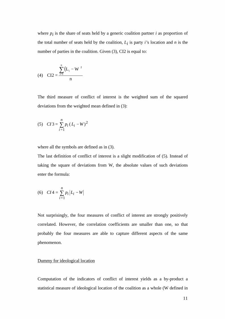
where pi is the share of seats held by a generic coalition partner i as proportion of
the total number of seats held by the coalition, Li is party i’s location and n is the
number of parties in the coalition. Given (3), CI2 is equal to:
(4) ( )
n
WL2CI
n
1i
2i∑
=
−=
The third measure of conflict of interest is the weighted sum of the squared
deviations from the weighted mean defined in (3):
(5) CI p L Wi ii
n3 2
1= −
=∑ ( )
where all the symbols are defined as in (3).
The last definition of conflict of interest is a slight modification of (5). Instead of
taking the square of deviations from W, the absolute values of such deviations
enter the formula:
(6) CI p L Wi ii
n4
1= −
=∑
Not surprisingly, the four measures of conflict of interest are strongly positively
correlated. However, the correlation coefficients are smaller than one, so that
probably the four measures are able to capture different aspects of the same
phenomenon.
Dummy for ideological location
Computation of the indicators of conflict of interest yields as a by-product a
statistical measure of ideological location of the coalition as a whole (W defined in
12
equation (3)). The measure W is statistical in the sense that it considers only the
location of parties and their weight in the coalition, it does not look at the
allocation of portfolios amongst partners, which is probably a key factor in
determining the effective ideological location of the cabinet. The construction of an
additional data set of real ideological locations of cabinets is currently in progress.
However, the statistical ideological location is itself of interest and it will play quite
a significant role in the two econometric applications proposed in the next sections.
The data set contains the measure W for each cabinet. In addition to that, a dummy
variable is defined, which takes value 1 for cabinets whose W is to the right of the
median location 5.5.
Total portfolio volatility, party portfolio volatility and within party reshuffles.
Huber (1998) argues that portfolios volatility might play a relevant role in shaping
the process of policy formation. With high volatility, ministers stay in office for a
relatively short time and thus they do not have the time to build up much
knowledge and expertise. Senior civil servants, instead, experience a much lower
turnover and they are bale to accumulate valuable information they might decide
not to share with ministers. Thus high volatility of portfolios is regarded as a
potential reason for "bad decisions" to be made.
Total portfolio volatility is therefore computed by comparing the allocation of
portfolios between two successive cabinets. Such a comparison can highlight five
different situations: (a) a portfolio is assigned to the same minister who was in
control of it in the outgoing cabinet, (b) a portfolio is assigned to a new minister
who belongs to the same party of the outgoing minister, (c) the new minister is not
of the same party as the old minister, (d) a portfolio is eliminated, (e) a new
portfolio is added. With the exception of (a), all other events give rise to some
form of volatility. However there is a clear difference between (b) and (c).In the
first case, it is likely that some kind of information spillover will take place between
13
the two ministers of the same party (they share the same ideology so they should
co-operate 12). In the second case, especially if the two parties are located far away
from each other on the ideological scale, the extent of information spillover will be
very limited. According to this argument, two different measures of volatility are
computed. Total portfolio volatility is the sum of (i) the number of changes in
individuals controlling portfolios (independently from the partisanship of the two
ministers), (ii) the number of portfolios eliminated, (iii) the number of portfolios
added. In party portfolio volatility the term in (i) is replaced by the number of
changes in the party controlling portfolios. The difference between total portfolio
volatility and party portfolio volatility is the number of within party reshuffles.
Ideological portfolio volatility
This measure combines the information on ideological location of parties with the
information on portfolios volatility. It has been used by Huber (1998) and it is the
sum of the Euclidean ideological distances for each portfolio change divided by the
total number of portfolios transferred. Consider the following example. Cabinet 17
in Austria (Vranitzky I) was supported by a coalition SPÖ/FPÖ. The following
Cabinet 18 (Vranitzky II) was supported by a coalition SPÖ/ÖVP. Since there was
a change in the partisan composition of the coalition, it is likely that some
portfolios "flew" from FPÖ to ÖVP. Indeed, 2 portfolios (Deputy PM and
Defence) shifted from FPÖ to ÖVP. In addition to that, other changes were
observed: 4 from SPÖ to ÖVP (Education, Agriculture, Environment, Social
Affairs), 1 from FPÖ to SPÖ (Industry and Trade), 1 from FPÖ to a non-aligned
minister (Defence), 3 new cabinets were created and 2 eliminated. The ideological
scale for those years (1986-1987) was: SPÖ 3.7, ÖVP 6.27, FPÖ 7.12 (the fact
12This argument is particularly true if the party can be viewed as a unitary actor. If instead partiesare characterised by significant internal divisions, then the transmission of knowledge betweentwo ministers of different wings of the same party can be very difficult.
14
that these locations are different from those of the previous example should not be
surprising since parties tend to move on the left-right scale over time). For the
purpose of computing ideological portfolio volatility the shift to the non-aligned
minister and the 5 creations/eliminations are not relevant.13 Thus:
IPV = [1*(7.12-3.7) + 4*(6.27 - 3.7) + 2*(7.12 - 6.27)]/7 = 2.205
Duration, survival rate and time horizon
For each cabinet the duration in days, and the corresponding number of years, are
reported. Those data on duration are taken from Woldendorp et al. (1993) and
therefore their conventions about the definition of the date of constitution and the
date of termination of the cabinet are adopted. In short, the life of a cabinet starts
when the formal process of investiture is completed and terminates only when a
new cabinet is formed.14 However, in order to guarantee cross-country
comparability, duration data should be expressed as the proportion of days a
government lasted in relation to the maximum period between elections allowed by
the constitution. This ratio, which is called survival rate, is also included in the data
set..
A problem with the survival rate is that it does not account for the fact that the
time horizon of a cabinet not formed immediately after an election is often
considerably shorter than the maximum period between elections allowed by the
constitution. The effective time horizon is taken into considerable account by the
government when deciding over economic policies and it is therefore important to
provide information on it. The data set does contain this information in the form of
13It would be problematic to define the ideological location of a non-aligned minister. For newlycreated (eliminated) posts the start (arrive) of the ideological journey of the portfolio is missing.14 The convention about the date of termination follows from the fact that even after its politicaldeath, the outgoing cabinet usually stays in office as a caretaker government (often with powerslimited to ordinary administration) until the incoming cabinet is officially invested.

15
a level variable called time left and a ratio variable called time horizon. Time left is
given by the constitutionally established period between two elections minus the
time elapsing between the date of last elections and the date of constitution of the
government. Time horizon is the ratio between time left and the maximum
potential period between two elections.
Coalition experience and prime minister expertise
Going through the process of policy formation in complex political environments
requires some expertise. This can be accumulated in two forms. First, it can be
accumulated by the coalition as a whole: the longer the time the same coalition has
been in power, the more experienced the coalition itself is likely to be. This means
that relationships between partners are more likely to occur along well-known lines
of behaviour and thus within coalition conflicts should be less frequent. Second,
personal expertise accumulated by the prime minister is also likely to matter, given
that a process of learning by doing could be at work.
Two measures are computed in the data set. The first one is "Coalition Experience"
and it is equal to the cumulative duration of all previous governments controlled by
the same coalition. The second measure is "Prime Minister expertise" and it is
given by the cumulative duration of all previous governments headed by the same
prime minister. The two measures have been introduced by Mauro (1998)
following an argument put forward by Strom (1988).
Compatibility index
This is a simple index of compatibility between the share of votes and the share of
portfolios received by coalition partners. For each of the n partners of a coalition
the difference between the share of electoral support and the share of portfolios
controlled is computed. Then, the n differences for the n partners in the coalition
16
are added up. The index is expressed as a percentage and technically it falls in the
range [0 , 1.999]. The value 0 corresponds to the case where all the parties which
contested elections are included in the coalition and each party controls a share of
portfolios exactly equal to its share of votes. The value 1.999 is the extreme case
of a party receiving a very small share of votes (say 0.001%) and controlling all
portfolios. In fact, the effective range for the countries in the data set is [0.051 ,
0.889] with an average of 0.4704 and a standard deviation of 0.1349.
The policy implemented by a coalition government is the result of bargaining
amongst coalition partners over portfolios allocation. Carmignani (1999) discusses
some alternative models of bargaining. In spite of the differences in the extensive
form of the game and the design of the process, for all these models it seems to be
true that the outcome does not necessarily relate to the parliamentary size of the
actors involved. This implies that the preferences expressed by voters might well be
distorted and the policy outcome be rather different from what would be obtained
in an hypothetical direct democracy where citizens choose policies without the
intermediation of representatives or political parties. The compatibility index is
meant at capturing such a distortion. However, some caveats must be stressed. For
example, an electorally small party could be able to hold out for the control of just
one, but key portfolio. If this is really the case, then this party would be able to
influence the policy of the coalition to a considerable extent, in spite of the fact that
its aggregate share of portfolios is small (and hence consistent with the small share
of votes received in the elections). Thus, voters’ preferences could be frustrated
even when the share of portfolios allocated to each partner roughly reflects the
share of votes that party received. Moreover, the distribution of voters’
preferences on each dimension of the policy space could be only imperfectly
approximated by the distribution of votes, so that an allocation of portfolios that
somehow reflects the distribution of votes could in fact be an imperfect
representation of citizens’ preferences on some dimensions.
17
MEASURES RELATED TO THE LEGISLATURE AS A WHOLE
Effective number of parties and fragmentation of the legislature
These two measures are based on the same equations (1) and (2) previously
defined with regard to the coalition. Now, all parties with parliamentary
representation are included and not just coalition partners. More fragmented
legislature are usually believed to generate more fragmented coalitions. Moreover,
a large effective number of parties implies that several different viable coalitions
can be formed at any time. The existence of such a large number of alternatives can
make the incumbent government more "fragile" in the sense of increasing the
likelihood of votes of no-confidence to be cast and/or by making partners' threat to
withdraw support and join in another of the several possible coalitions more
credible.
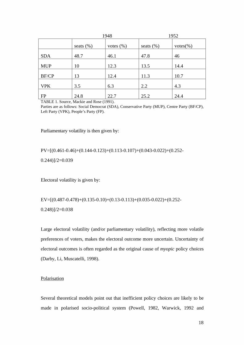
Electoral Volatility and Parliamentary Volatility.
Powell (1982) defines volatility of the party support as the sum of the share of
votes (electoral volatility) or seats (parliamentary volatility) added or lost by each
party in present elections respect to the previous contest, divided by two. Parties
which contest only one elections add their entire share of seats or votes. As an
example consider the definition of volatility for the third legislature in Sweden
(1952). Previous elections had been held in 1948. In both electoral contests only
five parties competed and received seats. Electoral results and share of seats are
reported in the Table 1 below:
18
1948 1952
seats (%) votes (%) seats (%) votes(%)
SDA 48.7 46.1 47.8 46
MUP 10 12.3 13.5 14.4
BF/CP 13 12.4 11.3 10.7
VPK 3.5 6.3 2.2 4.3
FP 24.8 22.7 25.2 24.4TABLE 1. Source, Mackie and Rose (1991).Parties are as follows: Social Democrat (SDA), Conservative Party (MUP), Centre Party (BF/CP),Left Party (VPK), People’s Party (FP).
Parliamentary volatility is then given by:
PV=[(0.461-0.46)+(0.144-0.123)+(0.113-0.107)+(0.043-0.022)+(0.252-
0.244)]/2=0.039
Electoral volatility is given by:
EV=[(0.487-0.478)+(0.135-0.10)+(0.13-0.113)+(0.035-0.022)+(0.252-
0.248)]/2=0.038
Large electoral volatility (and/or parliamentary volatility), reflecting more volatile
preferences of voters, makes the electoral outcome more uncertain. Uncertainty of
electoral outcomes is often regarded as the original cause of myopic policy choices
(Darby, Li, Muscatelli, 1998).
Polarisation
Several theoretical models point out that inefficient policy choices are likely to be
made in polarised socio-political system (Powell, 1982, Warwick, 1992 and
19
Alesina and Drazen, 1991). A quantitative definition of polarisation has been
proposed by Powell (1982). This is given by the total share of support expressed
by voters for "extremist" parties; that is, for those parties whose ideological
orientation is towards a radical change of the existing system. Based on the original
definition of extremism as well as on the country-specific list of extremist parties
provided by Powell for the '60s and the '70s, an updated list of parties whose share
of votes have to be included in the index of polarisation has been compiled. This
covers the whole post-war era and makes use of the information incorporated in
the new sources available since early '80s. For each country, at the time of each
general election, the index of polarisation includes the share of votes received by
parties which fall in at least one of the five following categories: (i) parties
explicitly labelled as Communists or Neo-Fascists, (ii) parties included in the
original list provided by Powell, (iii) parties whose ideological orientation is
explicitly independentist (for example, this is the case of the Northern League in
Italy in 1992, 1994 and 1996), (iv) parties located to the right of 8.5 or to the left
of 2.5 on the ten points ideological scales which are to be discussed in the
Appendix, (v) parties whose ideological orientation as stated in Political Parties of
the World (Keesings Publication, 1986) is unambiguously extremist in the original
definition given by Powell.
General Instability and Partisan Cabinet Instability
Probably, the simplest common sense idea of instability is represented by the
frequency of observed cabinet terminations. Huber (1998) suggests how to
incorporate this simple idea in two quantitative indicators. The indicator of General
Instability is given by the annual average number of terminations observed between
two elections. The indicator of Partisan Cabinet Instability is equal to the annual
average number of changes in the partisan composition of the cabinet. A few
technical details in the computation of these two measures are worth stressing.
20
With regard to the measure of General Instability, it has to be noticed that not all
terminations should be taken as a symptom of instability. Woldendorp et al (1993)
identify six possible reasons for termination: (a) elections, (b) voluntary
resignation of the prime minister, (c) resignations of the prime minister due to
health reasons, (d) dissension within the cabinet, (e) lack of parliamentary support,
(f) intervention by the Head of the State. Obviously, terminations (b), (c), (d) and
(f) must be included in the computation of the index. Terminations due to health
reasons (c), instead, should not be included because they have nothing to do with
the idea of cabinet instability or political instability. More subtle is the inclusion of
terminations falling in group (a). On the one hand scheduled mandatory elections
constitute a compulsory endpoint in the life of a cabinet. A cabinet could well
survive beyond the date of elections, but in parliamentary democracies the
incumbent has to resign when a new parliament is formed. Thus, life of cabinets is
censored when elections are held. On the other hand, elections are often
anticipated (that is, held before the end of the constitutionally established term).
Usually anticipated elections are held whenever a government is confronted with
either a no-confidence vote or internal dissension and no alternative coalition is
viable. Therefore, when caused by anticipated elections, cabinet terminations do
seem to represent a form of instability and they should be included in the
computation of the index of instability.15
The second technical point relates to the computation of the measure of Partisan
Cabinet Instability. When general elections intervene between two successive
governments, the change in the partisan composition of the coalition is imputed to
the new legislature. The rationale behind this choice is that the outgoing cabinet
usually stays in office (possibly with only limited powers) until the incoming one is
formed. Thus, the formal switch from the old partisan composition to the new one
takes place under the new legislature.
15 Elections are not considered anticipated if they are held within the six months before theconstitutionally established term.
21
Duration and survival rate of the legislature
As for cabinets, duration and survival of the legislature are reported in the data set.
Duration is expressed in days and fraction of years, survival is simply the ratio
between effective duration and maximum constitutionally established term.
Institutional dummy variables.
To account for cross-country differences in constitutional factors concerning
government cycles, three dummy variable are included in the data set. The
dummies are based on the discussion proposed by Laver and Schofield (1990, chp.
4). The first dummy (Investiture) takes value one if a formal investiture vote is
needed (as in Belgium, Ireland and Italy, for example) and zero otherwise. The
second dummy (government power) takes value one if the government can
dissolve the legislature (as it is commonly the case with the notable exception of
Norway and Finland) and zero otherwise. Finally the third dummy (legislature
power) takes value one if the legislature can dissolve itself (as it is the case in
Austria) and zero otherwise.
Section 2: Econometric analysis of determinants of cabinet duration.
The first of the two econometric applications proposed as an example of how the
political data set of Section 1 can be used is aimed at identifying the determinants
of cabinets duration. Short durations (which lead to high government turnover) are
often regarded as the key indicators of political instability (see Alesina et al. 1996
inter alia). Theoretical arguments suggest that various political, institutional and
economic variables are likely to have a significant impact on cabinet survival. A
22
very good survey of the theoretical as well as empirical results achieved in this field
of research can be found in Grofman and Van Roozendaal (1997).
Duration data are peculiar for two reasons. First of all, they can never take
negative values. The standard assumption of normality of the data is thus violated.
A possibility would be to assume log-normality (Greene, 1993). However, this
strategy does not overcome the second, more fundamental, issue: cabinet duration
are often in the nature of censored observations. Right-censoring occurs when the
cabinet terminates either because mandatory, non-anticipated elections are held or
because of resignation of the Prime Minister motivated by health problems. Notice
that terminations due to anticipated elections do not give rise to censored
observations. In effect, whilst non-anticipated elections represent a constitutionally
established deadline, independent from political conditions (i.e. the cabinet might
well have survived longer, had these elections not taken place), anticipated
elections do reflect a political stalemate involving the executive and the legislature.
In other words, anticipated elections are a symptom of political instability and
hence the associated cabinet terminations have to be treated as non-censored
observations.
Because of these peculiarities, the econometric analysis of cabinet duration data
requires the use of a specific statistical tool, known as event-history analysis (or
duration analysis). Such an approach was originally developed in biology and
engineering and more recently it has been applied to the study of economic
phenomena such as the duration of unemployment (Lancaster, 1979; Nickell, 1979;
Taylor, 1999) or labour disputes (Kennan, 1985). Kiefer (1988) surveys several
applications of duration models to economic problems.
The rest of this section is organised in two sub-sections. The first one contains a
(short) presentation of the specific econometric method used for the analysis. In
the second sub-section results of the analysis are discussed (Tables with all the
econometric results are reported in Appendix 2).

23
Partial Likelihood estimation of the proportional hazards model
The history of a generic cabinet i in a multiparty democracy can be represented as a
simple single-spell duration model known as "death process". This is a stochastic
process Xt which takes its values in the discrete space {E0, E1}. At time t = 0 (the
birth date) the process is in state E0. Transition to state E1 occurs just once in a
lifetime at time τ (the death date). The state E0 corresponds to the state "in office"
for the incumbent government and the transition to state E1 represents the
termination of the cabinet. T, the time period spent in state E0, is the duration of
the cabinet and it is in the nature of a positive random variable.
Of particular interest for duration analysis is the probability that a spell will be
completed at time t + ∆, given that it has lasted until time t. Such probability is
defined as:
(7) λ( ) limtP t T t T t
=< < + ≥
→∆
∆
∆0
λ(t) is called hazard function and it can be interpreted as the probability of
observing a change of status at time t (namely, between t and t + ∆).
The hazard function is used to characterise a process in terms of duration
dependence. If the derivative of λ(t) w.r.t. time, evaluated at t = t*, is positive,
then the process is said to exhibit positive duration dependence at t*. If instead the
derivative is negative, then the process exhibits negative duration dependence. The
notion of duration dependence is quite important when considering cabinet
duration. Positive duration dependence would imply that the probability of
observing a termination at same point t* increases the more distant t* is from the
birth date. This would mean that the longer a government has been in office, the
more likely it is to terminate in the near future. On the contrary, negative duration
24
dependence would imply that the longer the tenure of the cabinet, the less likely it
is to terminate in the near future.
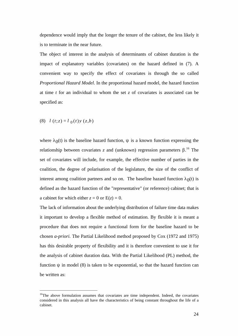
The object of interest in the analysis of determinants of cabinet duration is the
impact of explanatory variables (covariates) on the hazard defined in (7). A
convenient way to specify the effect of covariates is through the so called
Proportional Hazard Model. In the proportional hazard model, the hazard function
at time t for an individual to whom the set z of covariates is associated can be
specified as:
(8) λ λ ψ β( ; ) ( ) ( , )t z t z= 0
where λ0(t) is the baseline hazard function, ψ is a known function expressing the
relationship between covariates z and (unknown) regression parameters β.16 The
set of covariates will include, for example, the effective number of parties in the
coalition, the degree of polarisation of the legislature, the size of the conflict of
interest among coalition partners and so on. The baseline hazard function λ0(t) is
defined as the hazard function of the "representative" (or reference) cabinet; that is
a cabinet for which either z = 0 or E(z) = 0.
The lack of information about the underlying distribution of failure time data makes
it important to develop a flexible method of estimation. By flexible it is meant a
procedure that does not require a functional form for the baseline hazard to be
chosen a-priori. The Partial Likelihood method proposed by Cox (1972 and 1975)
has this desirable property of flexibility and it is therefore convenient to use it for
the analysis of cabinet duration data. With the Partial Likelihood (PL) method, the
function ψ in model (8) is taken to be exponential, so that the hazard function can
be written as:
16The above formulation assumes that covariates are time independent. Indeed, the covariatesconsidered in this analysis all have the characteristics of being constant throughout the life of acabinet.
25
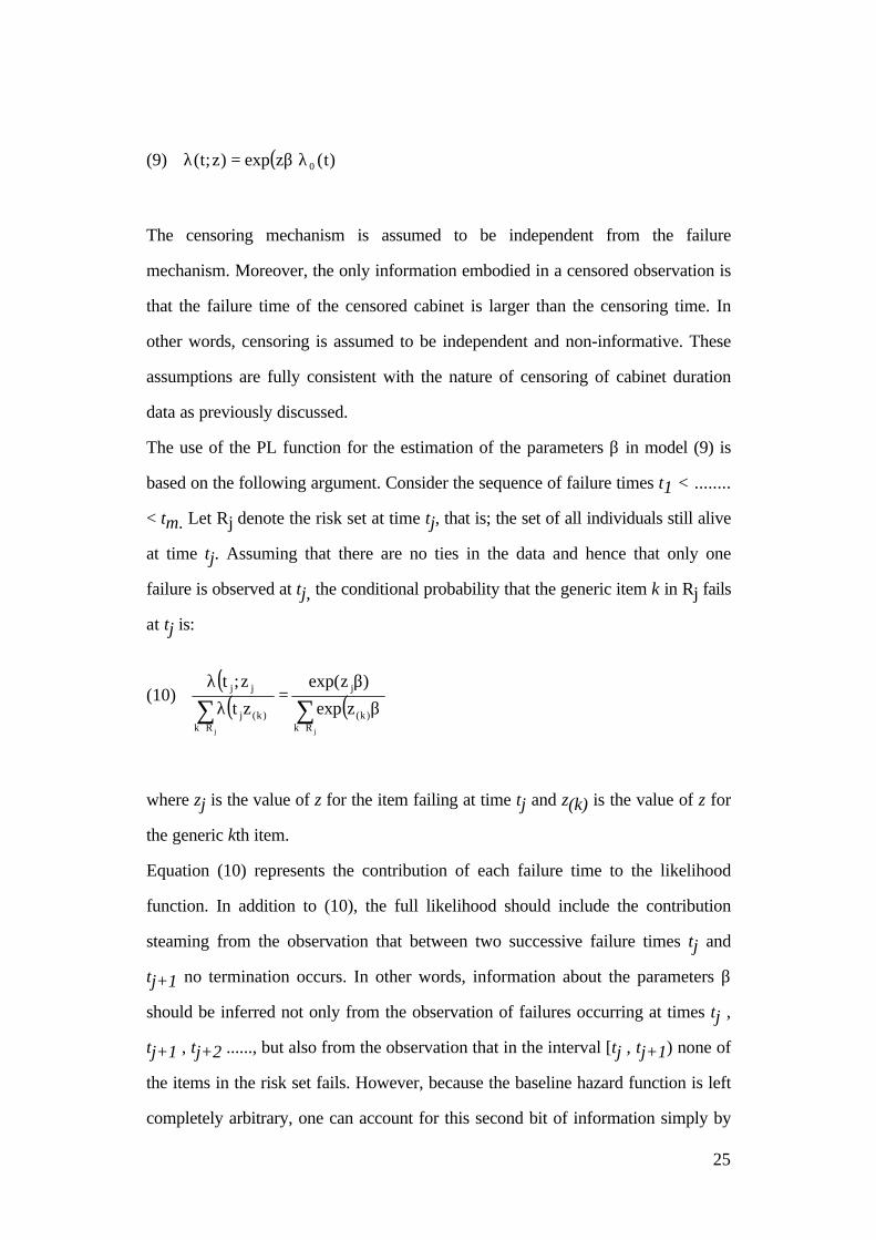
(9) ( ) )t(zexp)z;t( 0λβ=λ
The censoring mechanism is assumed to be independent from the failure
mechanism. Moreover, the only information embodied in a censored observation is
that the failure time of the censored cabinet is larger than the censoring time. In
other words, censoring is assumed to be independent and non-informative. These
assumptions are fully consistent with the nature of censoring of cabinet duration
data as previously discussed.
The use of the PL function for the estimation of the parameters β in model (9) is
based on the following argument. Consider the sequence of failure times t1 < ........
< tm. Let Rj denote the risk set at time tj, that is; the set of all individuals still alive
at time tj. Assuming that there are no ties in the data and hence that only one
failure is observed at tj, the conditional probability that the generic item k in Rj fails
at tj is:
(10) ( )
( ) ( )∑∑∈∈
β
β=
λ
λ
jj Rk)k(
j
Rk)k(j
jj
zexp
)zexp(
zt
z;t
where zj is the value of z for the item failing at time tj and z(k) is the value of z for
the generic kth item.
Equation (10) represents the contribution of each failure time to the likelihood
function. In addition to (10), the full likelihood should include the contribution
steaming from the observation that between two successive failure times tj and
tj+1 no termination occurs. In other words, information about the parameters β
should be inferred not only from the observation of failures occurring at times tj ,
tj+1 , tj+2 ......, but also from the observation that in the interval [tj , tj+1) none of
the items in the risk set fails. However, because the baseline hazard function is left
completely arbitrary, one can account for this second bit of information simply by
26
taking λ0(t) to be very close to zero in the interval [tj , tj+1). In this way, no
contribution needs to be registered from the observation that between any two
failure times no termination is occurred. In the end, the likelihood is formed by
taking the product over all failure times of (10) and it is in the nature of a Partial
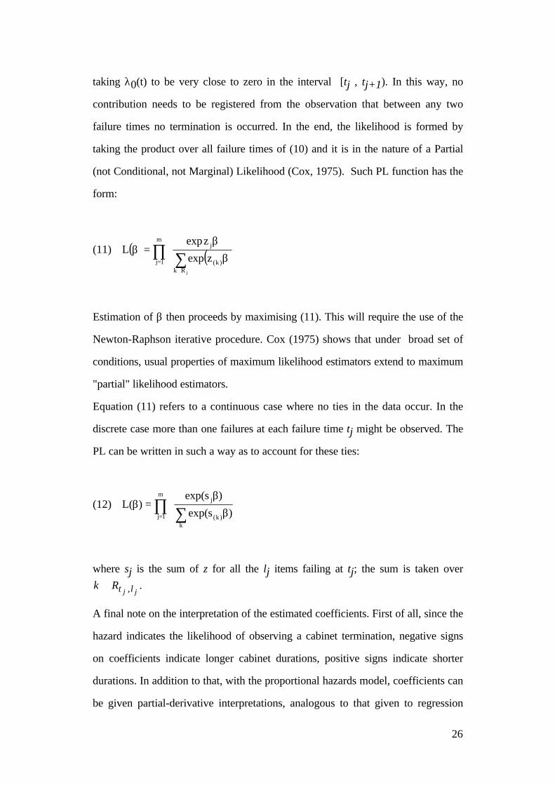
(not Conditional, not Marginal) Likelihood (Cox, 1975). Such PL function has the
form:
(11) ( ) ( )∏ ∑=∈
β
β=β
m
1jRk
)k(
j
j
zexp
zexpL
Estimation of β then proceeds by maximising (11). This will require the use of the
Newton-Raphson iterative procedure. Cox (1975) shows that under broad set of
conditions, usual properties of maximum likelihood estimators extend to maximum
"partial" likelihood estimators.
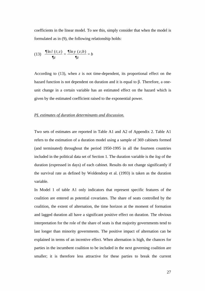
Equation (11) refers to a continuous case where no ties in the data occur. In the
discrete case more than one failures at each failure time tj might be observed. The
PL can be written in such a way as to account for these ties:
(12) ∏ ∑=
β
β=β
m
1jk
)k(
j
)sexp(
)sexp()(L
where sj is the sum of z for all the lj items failing at tj; the sum is taken over
k Rt lj j∈ , .
A final note on the interpretation of the estimated coefficients. First of all, since the
hazard indicates the likelihood of observing a cabinet termination, negative signs
on coefficients indicate longer cabinet durations, positive signs indicate shorter
durations. In addition to that, with the proportional hazards model, coefficients can
be given partial-derivative interpretations, analogous to that given to regression
27
coefficients in the linear model. To see this, simply consider that when the model is
formulated as in (9), the following relationship holds:
(13) ∂ λ
∂∂ ψ β
∂β
ln ( ; ) ln ( ; )t z
z
z
z= =
According to (13), when z is not time-dependent, its proportional effect on the
hazard function is not dependent on duration and it is equal to β. Therefore, a one-
unit change in a certain variable has an estimated effect on the hazard which is
given by the estimated coefficient raised to the exponential power.
PL estimates of duration determinants and discussion.
Two sets of estimates are reported in Table A1 and A2 of Appendix 2. Table A1
refers to the estimation of a duration model using a sample of 369 cabinets formed
(and terminated) throughout the period 1950-1995 in all the fourteen countries
included in the political data set of Section 1. The duration variable is the log of the
duration (expressed in days) of each cabinet. Results do not change significantly if
the survival rate as defined by Woldendorp et al. (1993) is taken as the duration
variable.
In Model 1 of table A1 only indicators that represent specific features of the
coalition are entered as potential covariates. The share of seats controlled by the
coalition, the extent of alternation, the time horizon at the moment of formation
and lagged duration all have a significant positive effect on duration. The obvious
interpretation for the role of the share of seats is that majority governments tend to
last longer than minority governments. The positive impact of alternation can be
explained in terms of an incentive effect. When alternation is high, the chances for
parties in the incumbent coalition to be included in the next governing coalition are
smaller; it is therefore less attractive for these parties to break the current

28
agreement and make the cabinet fall. The result concerning the time horizon
suggests that the first cabinet of a legislature is expected to last longer than
possible subsequent cabinets of the same legislature. However, since lagged
duration increases government’s survival, a “duration contagion”17 effect is also at
work and subsequent cabinets might benefit from it.
A significative negative impact on duration can be traced back to the effective
number of parties (ENP) in the coalition and to the degree of total portfolio
volatility (TPV). Indeed, in a more fragmented coalition (i.e. a coalition composed
of a large effective number of parties) internal conflicts are more likely to arise,
thus imposing a substantive constraint on the possibility of long durations. It is less
straight-forward to explain the impact of total portfolio volatility. A possible
argument goes as follows. With a high ministers turnover, each minister can
accumulate only little knowledge of the working of its portfolios (i.e. bureaucratic
structure, departmental activities, previously undertaken actions, and so on) and
this can push her to carry out "wrong" policies (or maybe, "right" policies in the
"wrong" way). Therefore, these mistakes made by individual ministers might
threaten the survival of the cabinet as a whole and determine shorter durations.
Model 2 includes as covariates only variables which refer to the legislature as a
whole. The rate of survival of the legislature has a strong positive effect on cabinet
duration. Thus a more stable legislature seems to be able to generate a more stable
cabinet. Not surprisingly, the degree of polarisation of the legislature strongly
reduces cabinet duration. High polarisation is an indicator of fierce political
competition. In such a difficult political environment, the chances to observe
cabinet terminations are increased. Finally, the degree of concentration of the
opposition does have a significant positive impact on duration. There are two ways
in which this result can be interpreted. The first one is that a strong opposition may
encourage coalition cohesion if coalition partners are afraid to let the opposition
17 This term has been originally proposed by Strom (1988).

29
into power. The second one is that concentrated oppositions are more likely to act
responsibly and play a constructive role in the process of policy formation, thus
“supporting” the cabinet.
Model 3 combines the previous two models. In this "full" political model almost all
coefficients retain the same sign they had in Model 1 and 2.18 Of particular interest
is the finding that the dummy variable for ideological location (location) has a
significant negative coefficient. To interpret this result, recall that the dummy takes
value one for cabinets located to the right of the median value 5.5 on the
ideological space [1, 10] and that a negative coefficient reflects a positive impact
on expected duration. Therefore, the model suggests that “right-wing” coalition
tend to last longer than “left-wing” coalitions.
Table A2 reports estimate of politico-economic models of duration. That is, some
economic variables have been added to the purely political specifications of Table
A1. The theoretical literature on the political business cycle and the partisan
business cycle19 makes use of models based on the expectations augmented Phillips
curve to formalise the interactions between economic and political cycles. It is
therefore reasonable to consider inflation and production as the two economic
variables which are most likely to influence cabinet duration. Unfortunately, the
monthly series of the Consumer Price Index (CPI) and the Industrial Production
Index (IP) made available by IMF/International Financial Statistics do not cover
the whole period 1950-1995 for all the 14 countries in the political data-set.
Therefore, the sample used to estimate the politico-economic models of duration
has to be restricted to 173 observations.
Model 4 of Table A2 is the full political model re-estimated for the smaller sample.
For some of the variables, results are quite different from those obtained in Model
18 The only exceptions concern the variable measuring the cumulative duration of all previousgovernment headed by the same Prime Minister (cumulative prime minister) and thecompatibility index. However, both are largely insignificant.19 See Alesina, Roubini and Cohen (1997) for a survey of contributions in this field.
30
3 of Table A1. However, for some other variables results are quite robust: the
potential time left at the moment of formation, the rate of survival and the degree
of polarisation of the legislature retains their significance as well as the sign of their
effect. In addition, two new variables become significant: the degree of conflict of
interest and the compatibility index both act in the sense of reducing duration. High
values of the compatibility index are indicators of low compatibility between
portfolios allocation and preferences expressed by voters (in the sense specified in
Section 1). Thus the negative impact on duration should not be surprising.
Similarly, high values of the index of conflict of interest imply significant
ideological differences between coalition partners. Again, such ideological diversity
is likely to cause early terminations.
In Model 5 of table 2 the "levels" of industrial production and inflation are included
as covariates. This does not significantly alter the sign and the significance of the
political variables. Moreover, with the exception of polarisation, the size of the
coefficients of the five political variables which are strongly significant in the full
political model are not changed dramatically. The estimated coefficients of the two
economic variables are as expected. Higher inflation acts in the sense of shortening
duration, whilst higher industrial production increases the chances of survival. This
result implies that cabinet’s survival cannot be taken as being independent from
economic performance. In particular, the assumption (common to most models of
political and partisan business cycle) that poor economic performance (i.e. high
inflation, low production) will represent a burden for the incumbent only at the
time of next elections is too restrictive: poor economic performance is a liability
the incumbent might be called to pay for even before the constitutionally
established term of office has expired.
In Model 6 together with the levels of inflation and industrial production, the
volatility of inflation (measured as the standard deviation of inflation) and the
growth rate of industrial production are entered the full specification. In fact, these
two variables do not seem to add very much to the explanatory power of the
31
model. The relative large standard errors reported in the table implies that the
coefficients are not very precisely estimated.
Finally, Model 7 of Table 2 is aimed at testing whether or not the significant impact
of economic variables (expressed in levels) on duration is robust to institutional
differences across countries. For this purpose the three institutional dummy
variables presented in Section 1 are added to the specification. The dummy
legislature takes value one if the legislature can dismiss itself. The negative sign of
the estimated coefficient suggests that when such power is afforded to the
legislature, the duration of the cabinet is increased. The dummy government takes
value one if the government has the power to dismiss the legislature. As one would
expect, when such power is granted to the cabinet, the cabinet's probability of
survival increases. The existence of a formal investiture procedure (captured by the
dummy investiture) is on theoretical grounds less important for cabinet duration
and more relevant for the duration of the process of cabinet formation. The low
significance of its coefficient does confirm this theoretical point. In general, results
concerning the other political and economic variables are robust to adding
institutional dummies to the model.
Finally, the issue of time dependence can be addressed by looking at the curvature
of the integrated hazard function. The integrated hazard is defined as:
(14) ∫ λ=Λt
0du)u()t(
When plotted against duration, the integrated hazard function will be convex if the
hazard function is increasing w.r.t. time; that is, if there is positive duration
dependence. If instead the integrated hazard is concave, then the hazard function is
decreasing with duration and thus there is negative duration dependence. In all the
models of Table A1 and A2, plots of the integrated hazard (not reported) show a
clear positive duration dependence. As already pointed out, positive duration
dependence implies that the longer a cabinet stays in office, the higher the
32
probability it will collapse in the near future. This very same result has been found
by Merlo (1998) in his analysis of cabinet duration in Italy.
Section 3. Political determinants of government consumption expenditure.
The idea that political instability has significant impact on the size and the
composition of government expenditure and, via government expenditure, on the
overall economic performance of the system is incorporated in several models
(Darby, Li, Muscatelli, 1998; Alesina Perotti and Tabares, 1998; Sachs and
Roubini, 1989). The political data set presented in Section 1 allows for a
systematic analysis of political determinants of government consumption
expenditure. Of course, government consumption is likely to be determined not
just by political factors, but by economic and environmental factors as well. For
this reason, the panel models of Tables A3 and A5 include three “control”
variables: (i) the fertility rate (in log-form), (ii) the enrolment rate in higher
education, (iii) the level of per-capita real GDP, adjusted for changes in the terms
of trade. The first is meant to capture the effect of a growing population on the
size of public consumption and current social expenditure. The second-one is
intended as a proxy for the demand of education infrastructure (which are often
provided by the government). Finally, the level of per capita GDP is used as
indicator of wealth: in richer countries government expenditure should be higher,
other things being equal.20
The dependent variable is the ratio of real government consumption expenditure to
real GDP observed in each of the 14 countries of the political data set over the
sample period 1965-1990. All data are averaged over periods of five years. For
political variables, a weighted average is computed as follows. Each cabinet which
20 Data on fertility are taken from various issues of the Statistical Yearbook of United Nations, theenrolment rate is taken from the Barro and Lee data set (1993) and the data on the level of realper-capita GDP are from Summer and Heston (1991).
33
stayed in office over a fraction of each quinquennium is assigned a weight equal to
the ratio of its duration (in days) to the total number of days in a quinqiennium (i.e.
1800). For cabinets that stayed in office across two successive quinquennia, only
the fraction of duration falling in the quinquennium of interest is used to determine
the weight. Once weights are determined, the political measures for each country in
each quinquennium are simply the weighted average of the data observed for each
cabinet in office for any fraction of the quinquennium. Exceptions to this procedure
are made for the measures of portfolio volatility (Total Portfolio Volatility, Party
Portfolio Volatility and Ideological Portfolio Volatility). For such measures simple
rather than weighted averages are computed.21 The measures of general instability
and partisan cabinet instability are obtained by counting the number of cabinet
terminations and changes in the partisan composition of the cabinet occurred over
each quinquennium and then dividing by 5 (so to obtain a yearly average over the
quinquennium).
The set of results in Table A3 refers to OLS estimation of the model. Model 1 of
Table A3 is a full politico-economic model, where all political variables plus the
three control variables are entered22. A few intriguing findings are worth
mentioning. First of all, the three control variables all have positive and significant
coefficients, as one would expect. Turning to the political variables, three of them
seem to have a particularly significant impact. Cabinet duration acts in the sense of
increasing government expenditure whilst both the share of seats controlled by the
coalition and the dummy for ideological location have a negative sign. The inverse
relationship between share of seats and government consumption is consistent with
21 The reason for this special treatment has to do with the specific nature of the three variables.Portfolio volatility is observed only once, at the moment of formation of the new cabinet. Instead,measures such as the effective number of parties in the coalition represent situations which areobserved continuously at any moment of the life of the cabinet. Therefore, it seems more plausibleto give the latter a weight as a function of the time the government stays in office, whilst portfoliovolatility measures are better represented by simple average.22In fact, not all the political variables of the data set are entered as regressors. The reason forthat is that some of them tend to be highly correlated and thus problems of multicollinearitymight arise.
34
the findings reported by Darby, Li and Muscatelli (1998). Indeed, theoretical
models predict that the share of seats controlled by the coalition, being an indicator
of political stability, should work in the sense of limiting the level of government
consumption. An analogous argument should apply to cabinet duration. To the
extent that it is possible to interpret duration as an indicator of stability, one would
expect lower government consumption associated to longer duration. The positive
sign of the coefficient of cabinet duration in Model 1 suggests that some other
effect is at work. In particular, it might well be possible that the ability or the
incentive "to spend" of cabinet ministers increases with tenure, thus making the
relationship between duration and government consumption positive. The finding
that the dummy for ideological location has a negative coefficient is very
interesting. It means that "left-wing" government effectively tend to increase
government consumption relatively to "right-wing" government.
Model 2 is the politico-economic model re-estimated with OLS after dropping the
variables that in Model 1 resulted highly insignificant. Now both the survival rate
of the legislature and the survival rate of the cabinet have significant negative
coefficients. This result is in contradiction with the finding that duration has a
positive impact on government consumption. This can probably be interpreted as a
further confirmation that, with regard to the time dimension of political instability,
several alternative mechanisms of influence on the process of policy formation are
at work. The negative sign of the coefficient of total portfolio volatility, however,
seems to support the idea that the ability to spend of ministers might be positively
related to tenure (or inversely related to turnover). The null hypothesis of zero
restrictions on the coefficient of the measure of fragmentation and the measure of
concentration of the opposition cannot be rejected at usual confidence level.
Therefore, Model 2 has been re-estimated after deleting such two variables,
yielding Model 3 in Table A3. Some additional specification tests are reported in
Table A4.
35
Table A5 contains Instrumental Variables estimation of Model 2 (without the index
of concentration of the opposition) and Model 3 in Table 3. There are good
reasons to believe that the three control variables might be endogenous. Therefore,
lagged values of the fertility rate, the enrolment rate in higher education and the
real per-capita GDP are used as instruments. It can be noticed that the main results
obtained with simple OLS still hold.
Conclusion.
The two econometric applications suggested in this paper are an example of the
vast range of possible applications for the political measures included in the data
set presented in Section 1. Some interesting results have been obtained.
The duration analysis of Section 2 shows that the probability for a government to
collapse increases the higher the degree of ideological heterogeneity of coalition
partners, the higher the degree of polarisation of the system, the lower the rate of
survival of the legislature, the shorter the time horizon to next mandatory elections
and the worse the overall economic conditions of the country. There is also
evidence of positive duration dependence: the longer the cabinet has stayed in
power, the higher the probability it will collapse in the near future.
The panel analysis of Section 3 suggests that once controlling for some economic
and environmental variables, political variables do have an impact on government
spending decisions. In particular, the ideology of the coalition matters: with left-
wing cabinets the level of government consumption expenditure tends to be higher
than with right-wing cabinets. Another intriguing finding is that higher portfolio
volatility reduces government consumption expenditure. This result supports the
view that the ability of individual ministers to obtain resources for their department
increases with ministers’ tenure.
36
Appendix 1. Left-Right ideological scales: sources and methods.
To compute the measures of conflict of interest, polarisation and ideologicalportfolio volatility, empirical policy scales reporting the cardinal location of partieson the left-right ideological continuum are needed. The construction of such scalesis usually based on either the analysis of electoral manifestos or country experts'judgement. In both cases the purpose is to collect information concerning theideological orientation of parties on different, relevant dimensions of the policyspace and then summarise such information by assigning each party a cardinallocation on a unidimensional space (the left-right scale). Obviously such anexercise has some intrinsic limitations, especially if the policy space consists ofseveral, heterogeneous dimensions. A party might well decide, for example, to be"liberal" with regard to the cultural-linguistic dimension, but "conservative" withregard to the economic dimension. Both the cultural-linguistic and the economicdimension are likely to be relevant and they should both contribute to determinethe overall position of the party on the unidimensional left-right continuum. Asystem of weights has to be used in such case, but especially for scales based onexperts' judgements, the choice of what weights to use might be arbitrary andconditioned by historical experiences of coalitions. However, two factorscontribute to rise the degree of reliability of information obtained from theempirical policy scales available in the literature. First of all, some authors (Laverand Shepsle, 1996b) note that party locations on different dimensions of the policyspace tend to be positively correlated. This means that cases of parties which are"liberal" on some issues and "conservative" on some other issues are more theexception than the norm. Second, there is still some wide agreement over theimportance of the economic dimension as the one involving the basic issues thatdivide left from right (Huber and Inglehart, 1995). Thus, even if the number ofdimensions composing the policy space is large, the economic orientation of theparty can be taken as being the key indicator of the ideological position of the partyitself. These are definitely good news for those economists who use empiricalpolicy scales to analyse the interaction between politics and economics.Several empirical left-right scales are available in the literature. Since parties tendto re-locate over time, it is convenient to make use of scales produced at differenttimes and to partition the post-war era so that the position of each party at a giventime is taken from the scale produced in the proximity of that time. Four basicsources are considered: Dodd (1976), Browne et al. (1984), Castles and Mair(1984), Huber and Inglehart (1995). In addition to those, some country-specificsources (such as Hardson and Kristens, 1987) are sometimes used to fill gaps leftin the four main sources. All scales are converted into a continuum spanning from1 (extreme left) to 10 (extreme right). The two points 2.5 and 8.5 are used asthresholds to identify extremist parties. These thresholds have been chosen on thebasis of the discussion in Dodd (1976). Dodd explicitly reports that extremistparties on his scales are located either to the left of -5 or to the right of +5.Converting the locations -5 and +5 onto the continuum spanning from 1 to 10 oneobtains 2.5 and 8.5. The median 5.5 is used as threshold to divide "left-wing" from"right-wing" coalitions and to construct the ideological dummy variable.
37
The advantage of using different scales to cover different fractions of the wholesample period can be illustrated with an example. In Italy commentators almostunanimously recognise that the PSI (Socialist Party) has experienced over the post-war era a significant ideological re-location from the left towards the centre. Suchre-location has been witnessed by the increasing importance of the role of PSI as acoalition partner of DC (Christian Democrats). Throughout late '70s, '80s and early'90s (until the dissolution of the old party system), PSI has constantly remainedmember of the broad government coalitions built around DC, often receivingimportant cabinets and holding the prime-ministership three times.23 The re-location process engaged by the PSI and its effects on the structure of Italiancoalitions and, more generally, Italian politics would not be fully accounted for bythe measures included in the political data set if a unique policy scale (possiblyobtained by applying discriminant analysis to the four main sources previouslymentioned) were used. In such a case, in fact, the location of parties would beassumed constant thorough time. Instead, by using the Dodd's scale for the firstsub-period (1945-1975), then the Castle and Mair's scale for the second sub-period(1975-1990) and then the Huber and Inglehart's scale for the third period (1990-1998), the ideological location of PSI used as the basis for the computation ofmeasures of conflict of interest and ideological portfolio volatility gradually movesfrom 3.5 to 3.8 to 5, consistently with what has been observed in the politicalarena. The same approach of "partition" of time has been used for all countries, sothat in general, parties re-location should be consistently captured by the indices inthe data set.All information regarding ideological location of parties is contained in 14"matrices of ideology" (one for each country). Each of such matrices is of size n*k,where n is the number of parties with parliamentary representation in at least oneof the post-war legislatures and k is the number of post-war cabinets. Thesematrices thus provide a complete overview of the ideological locations occupied byall parties involved in national politics in each of the fourteen countries of thesample.
23The importance of this event is clear if one considers that until 1993, 51 cabinets were formedin Italy. In 46 out of these 53 cases the prime-minister was a Christian Democrat and the onlytwo parties able to obtain the prime-ministership other than DC were PSI and PRI.
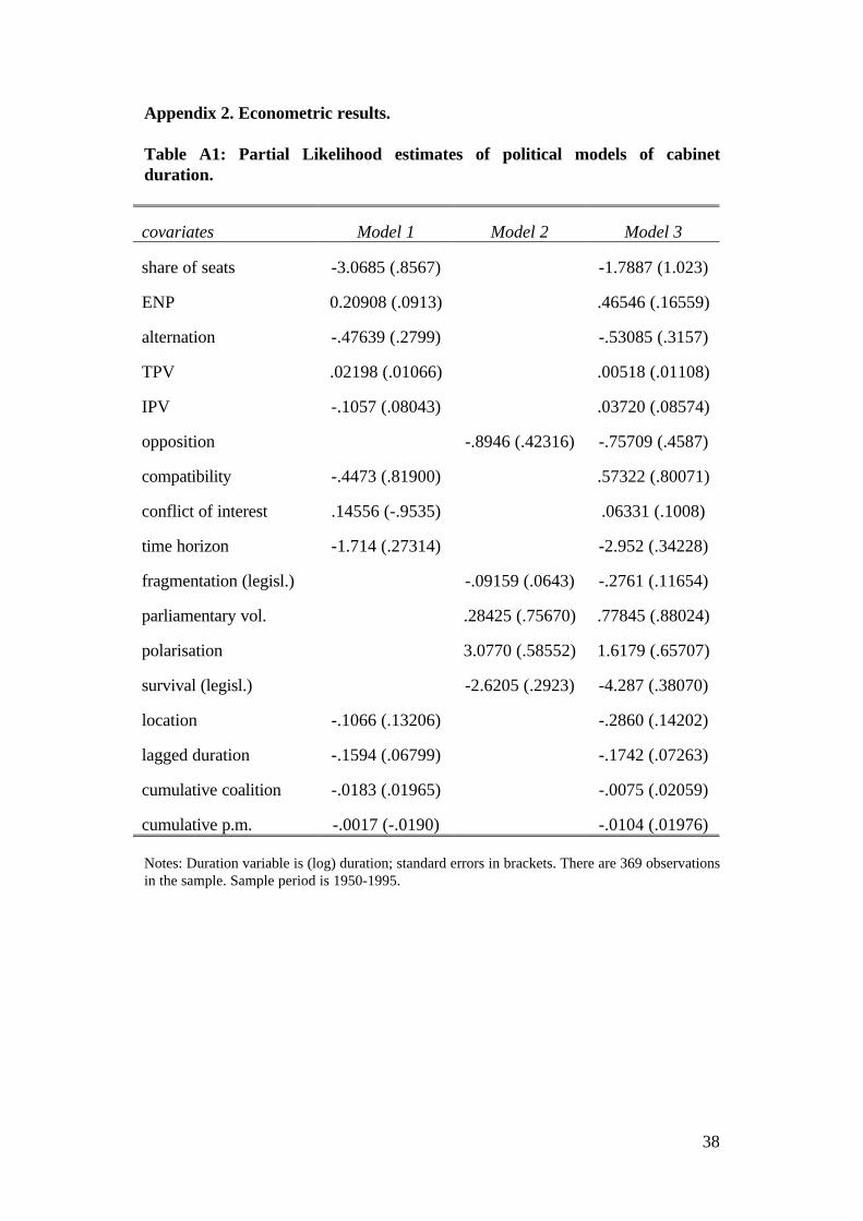
38
Appendix 2. Econometric results.
Table A1: Partial Likelihood estimates of political models of cabinetduration.
covariates Model 1 Model 2 Model 3
share of seats -3.0685 (.8567) -1.7887 (1.023)
ENP 0.20908 (.0913) .46546 (.16559)
alternation -.47639 (.2799) -.53085 (.3157)
TPV .02198 (.01066) .00518 (.01108)
IPV -.1057 (.08043) .03720 (.08574)
opposition -.8946 (.42316) -.75709 (.4587)
compatibility -.4473 (.81900) .57322 (.80071)
conflict of interest .14556 (-.9535) .06331 (.1008)
time horizon -1.714 (.27314) -2.952 (.34228)
fragmentation (legisl.) -.09159 (.0643) -.2761 (.11654)
parliamentary vol. .28425 (.75670) .77845 (.88024)
polarisation 3.0770 (.58552) 1.6179 (.65707)
survival (legisl.) -2.6205 (.2923) -4.287 (.38070)
location -.1066 (.13206) -.2860 (.14202)
lagged duration -.1594 (.06799) -.1742 (.07263)
cumulative coalition -.0183 (.01965) -.0075 (.02059)
cumulative p.m. -.0017 (-.0190) -.0104 (.01976)
Notes: Duration variable is (log) duration; standard errors in brackets. There are 369 observationsin the sample. Sample period is 1950-1995.
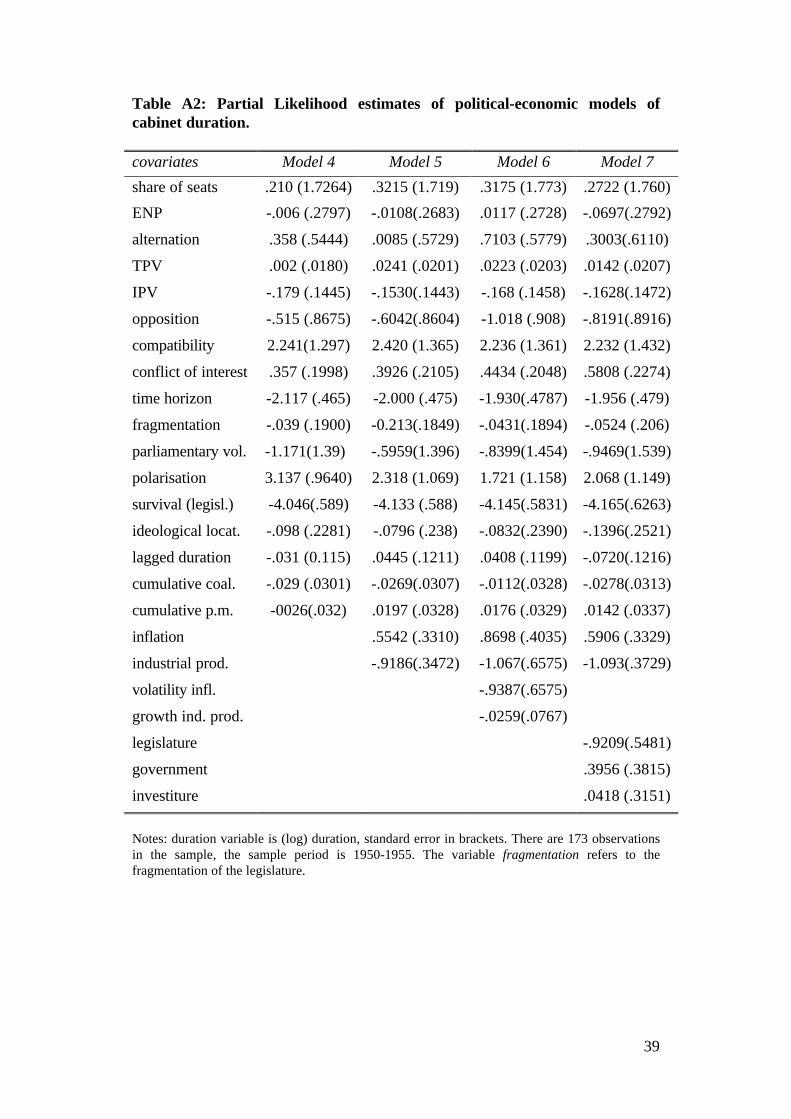
39
Table A2: Partial Likelihood estimates of political-economic models ofcabinet duration.
covariates Model 4 Model 5 Model 6 Model 7
share of seats .210 (1.7264) .3215 (1.719) .3175 (1.773) .2722 (1.760)
ENP -.006 (.2797) -.0108(.2683) .0117 (.2728) -.0697(.2792)
alternation .358 (.5444) .0085 (.5729) .7103 (.5779) .3003(.6110)
TPV .002 (.0180) .0241 (.0201) .0223 (.0203) .0142 (.0207)
IPV -.179 (.1445) -.1530(.1443) -.168 (.1458) -.1628(.1472)
opposition -.515 (.8675) -.6042(.8604) -1.018 (.908) -.8191(.8916)
compatibility 2.241(1.297) 2.420 (1.365) 2.236 (1.361) 2.232 (1.432)
conflict of interest .357 (.1998) .3926 (.2105) .4434 (.2048) .5808 (.2274)
time horizon -2.117 (.465) -2.000 (.475) -1.930(.4787) -1.956 (.479)
fragmentation -.039 (.1900) -0.213(.1849) -.0431(.1894) -.0524 (.206)
parliamentary vol. -1.171(1.39) -.5959(1.396) -.8399(1.454) -.9469(1.539)
polarisation 3.137 (.9640) 2.318 (1.069) 1.721 (1.158) 2.068 (1.149)
survival (legisl.) -4.046(.589) -4.133 (.588) -4.145(.5831) -4.165(.6263)
ideological locat. -.098 (.2281) -.0796 (.238) -.0832(.2390) -.1396(.2521)
lagged duration -.031 (0.115) .0445 (.1211) .0408 (.1199) -.0720(.1216)
cumulative coal. -.029 (.0301) -.0269(.0307) -.0112(.0328) -.0278(.0313)
cumulative p.m. -0026(.032) .0197 (.0328) .0176 (.0329) .0142 (.0337)
inflation .5542 (.3310) .8698 (.4035) .5906 (.3329)
industrial prod. -.9186(.3472) -1.067(.6575) -1.093(.3729)
volatility infl. -.9387(.6575)
growth ind. prod. -.0259(.0767)
legislature -.9209(.5481)
government .3956 (.3815)
investiture .0418 (.3151)
Notes: duration variable is (log) duration, standard error in brackets. There are 173 observationsin the sample, the sample period is 1950-1955. The variable fragmentation refers to thefragmentation of the legislature.
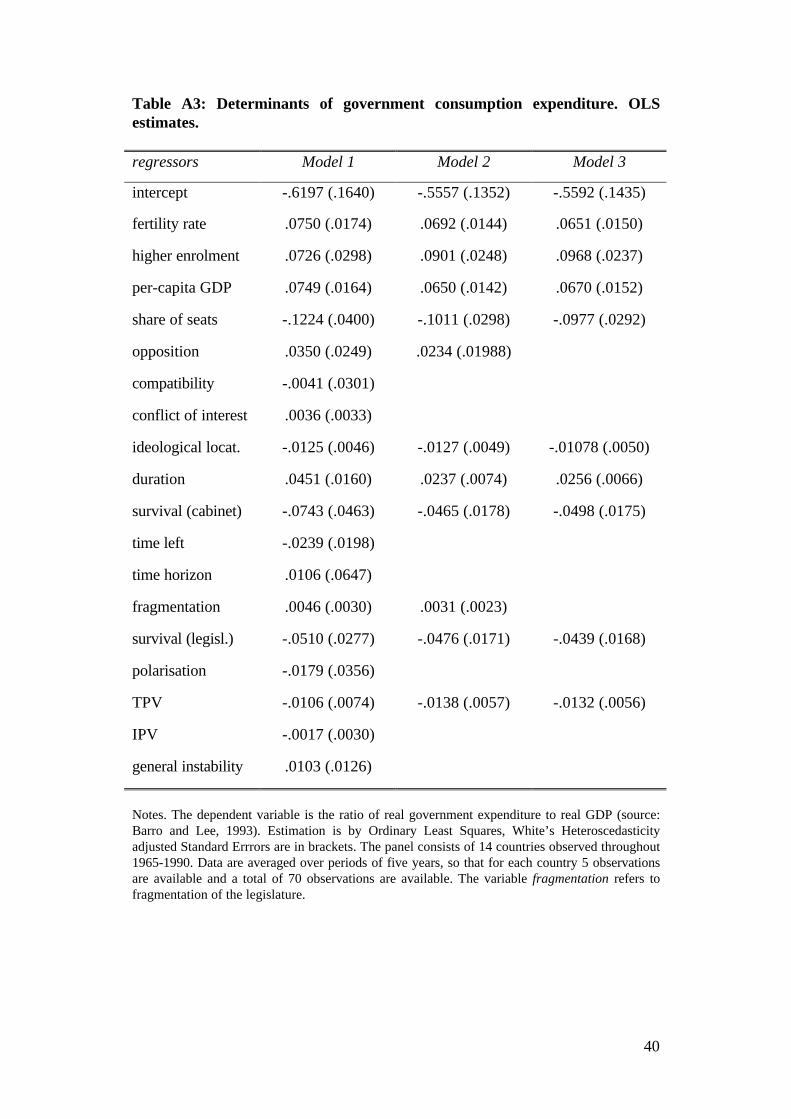
40
Table A3: Determinants of government consumption expenditure. OLSestimates.
regressors Model 1 Model 2 Model 3
intercept -.6197 (.1640) -.5557 (.1352) -.5592 (.1435)
fertility rate .0750 (.0174) .0692 (.0144) .0651 (.0150)
higher enrolment .0726 (.0298) .0901 (.0248) .0968 (.0237)
per-capita GDP .0749 (.0164) .0650 (.0142) .0670 (.0152)
share of seats -.1224 (.0400) -.1011 (.0298) -.0977 (.0292)
opposition .0350 (.0249) .0234 (.01988)
compatibility -.0041 (.0301)
conflict of interest .0036 (.0033)
ideological locat. -.0125 (.0046) -.0127 (.0049) -.01078 (.0050)
duration .0451 (.0160) .0237 (.0074) .0256 (.0066)
survival (cabinet) -.0743 (.0463) -.0465 (.0178) -.0498 (.0175)
time left -.0239 (.0198)
time horizon .0106 (.0647)
fragmentation .0046 (.0030) .0031 (.0023)
survival (legisl.) -.0510 (.0277) -.0476 (.0171) -.0439 (.0168)
polarisation -.0179 (.0356)
TPV -.0106 (.0074) -.0138 (.0057) -.0132 (.0056)
IPV -.0017 (.0030)
general instability .0103 (.0126)
Notes. The dependent variable is the ratio of real government expenditure to real GDP (source:Barro and Lee, 1993). Estimation is by Ordinary Least Squares, White’s Heteroscedasticityadjusted Standard Errrors are in brackets. The panel consists of 14 countries observed throughout1965-1990. Data are averaged over periods of five years, so that for each country 5 observationsare available and a total of 70 observations are available. The variable fragmentation refers tofragmentation of the legislature.

41
Table A4: Variable addition tests
Additional variables Lagrange Multiplierstatistic
Likelihood Ratio statistic
ENP .57284 (.449) .57519 (.448)
compatibility .069398 (.792) .069432 (.792)
conflict of interest .25133 (.616) .25178 (.616)
time left 1.4763 (.224) 1.4921 (.222)
polarisation 1.0546 (.304) 1.0626 (.303)
general instability .090221 (.764) .090279 (.764)
The basic specification is the one of Model 2, Table A3. The null hypothesis is stated as a zerorestriction on the coefficient of each of the additional variables listed above. Thus, variable shouldbe added to the basic specification if the test statistic is sufficiently high (and the null can berejected). P-values are reported in brackets. As it can be seen from the values reported in thesecond and in the third column, for none of the additional variables, the null hypothesis can berejected at usual confidence levels.The joint test of zero restrictions on the coefficients of the two variables opposition andfragmentation of the legislature yields the following results: Lagrange Multiplier Statistic 2.5096(.285); Likelihood Ratio Statistic 2.5557 (.279). Again, the null hypothesis cannot be rejected andhence the two variables can be deleted. Model 3 in Table A3 is Model 2 re-estimated afterdeleting the two variables.
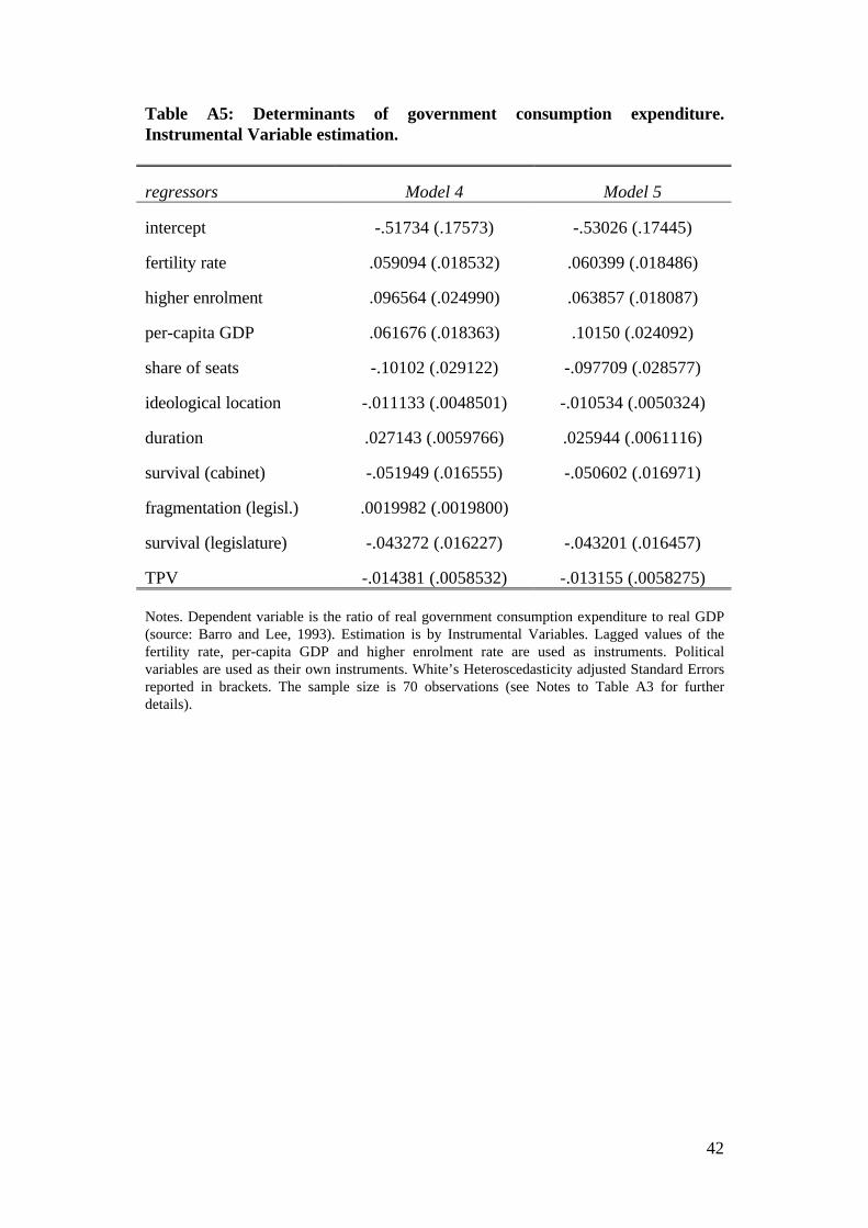
42
Table A5: Determinants of government consumption expenditure.Instrumental Variable estimation.
regressors Model 4 Model 5
intercept -.51734 (.17573) -.53026 (.17445)
fertility rate .059094 (.018532) .060399 (.018486)
higher enrolment .096564 (.024990) .063857 (.018087)
per-capita GDP .061676 (.018363) .10150 (.024092)
share of seats -.10102 (.029122) -.097709 (.028577)
ideological location -.011133 (.0048501) -.010534 (.0050324)
duration .027143 (.0059766) .025944 (.0061116)
survival (cabinet) -.051949 (.016555) -.050602 (.016971)
fragmentation (legisl.) .0019982 (.0019800)
survival (legislature) -.043272 (.016227) -.043201 (.016457)
TPV -.014381 (.0058532) -.013155 (.0058275)
Notes. Dependent variable is the ratio of real government consumption expenditure to real GDP(source: Barro and Lee, 1993). Estimation is by Instrumental Variables. Lagged values of thefertility rate, per-capita GDP and higher enrolment rate are used as instruments. Politicalvariables are used as their own instruments. White’s Heteroscedasticity adjusted Standard Errorsreported in brackets. The sample size is 70 observations (see Notes to Table A3 for furtherdetails).

43
References.
Alesina, A. and A. Drazen (1991). "Why are Stabilisation Delayed". AmericanEconomic Review, 81, 1170-1185
Alesina, A. , R. Perotti, J. Tavares (1998) "The Political Economy of FiscalAdjustments", Brookings Papers on Economic Activity, 1, 197-226.
Alesina, A. N. Roubini and G. Cohen (1997) Political Cycles and theMacroeconomy, The MIT Press.
Axlerod, R. (1970) Conflict of Interest Theory, Cambridge University Press.
Bellettini, G. (1998). "Aggregate Uncertainty, Political Instability and IncomeRedistribution", European Journal of Political Economy, 14, 19-33.
Browne, E.C. , D. Gleiber and C. Mashoba (1984) "Evaluating Conflict of InterestTheory: Western European Cabinet Coalitions, 1945-80", British Journal ofPolitical Studies, 14, 1-32.
Calvo, G. and A. Drazen (1997). "Uncertain duration of reform: dynamicimplications", NBER Working Paper 5925
Carmignani, F. (1999). “Theoretical Models of Bargaining over the Allocation ofPortfolios in Coalition Governments”, forthcoming Quaderni del dipartimento dieconomia politica series, Universita’ Cattolica del Sacro Cuore – Milano.
Castles, F. and P. Mair (1984), "Left-Right Political Scales: Some ExpertJudgements", European Journal of Political Research, 73-88.
Cox, D.R. (1972) "Regression Models and Life-Tables (with discussion)", Journalof the Royal Statistics Society, 1972, B 34, 187-220.
Cox, D.R. (1975) "Partial Likelihood", Biometrika, 62 (2), 269-76
Dalle Nogare, C. (1997). "Ideological Polarisation, Coalition Governments andDelays in Stabilisation", University of Glasgow, Department of EconomicsDiscussion Paper No. 9710
Darby, J. , C.W. Li and V.A. Muscatelli (1998). "Political Uncertainty, PublicExpenditure and Growth". University of Glasgow, Department of EconomicsDiscussion Paper No 9822.
Deveraux, M. and J.F.Wen (1996). "Political uncertainty, capital taxation andgrowth". Mimeo, University of British Columbia.
Dodd, L.C. (1976) Coalitions in Parliamentary Government, Princeton UniversityPress.
44
Greene, W.H. (1993) Econometric Analysis., 2nd ed., MacMillan.
Grofman, B. and P. Van Roozendaal (1997) "Review Article: Modelling CabinetDurability and Termination", British Journal of Political Studies, 27, 419-451.
Huber, J.D. (1998). "How Does Cabinet Instability Affect Political Performance ?Portfolio Volatility and Health Care Cost Containment in ParliamentaryDemocracies", American Political Science Review, Vol.92, No. 3.
Huber, J.D. and R. Inglehart (1998) "Expert Interpretations of Party Space andParty Locations in 42 Societies", Party Politics, 1, 73-111.
Laasko, M. and R. Taagepera (1979) "Effective Number of Parties: A Measurewith Application to West Europe", Comparative Political Studies, 12, 3-27.
Katz, P. and P. Mair (1990). Party Organisations.
Keesing's Archive Publication (1985) Political Parties of the World.
Kennan, J. (1985) "The Duration of Contract Strikes in U.S. Manufacturing",Journal of Econometrics, 28 (1), 5-28.
Kiefer, N.M. "Economic Duration Data and Hazard Functions", Journal ofEconomic Literature, Vol XXVI, 646-679.
Koele, R. and P. Mair (eds.) "Political Data Yearbook", European Journal ofPolitical Research, various issues.
Lancaster, T. (1979) "Econometric Methods for the Duration of Unemployment",Econometrica, 47 (4), 939-56.
Laver, M. and N. Schofield (1990) Multiparty Government, Oxford UniversityPress.
Laver, M. and K.A. Shepsle (1996a). Making and Breaking Governments,Cambridge University Press.
Laver, M. and K.A. Shepsle (1996b). Cabinet Ministers and ParliamentaryGovernments, Cambridge University Press.
Mackie, T. and R. Rose (1991) The International Almanac of Electoral History,MacMillan.
Mackie, T. and R. Rose (1997) A decade of Election Results: updating theinternational almanac, Centre for the Study of Public Policy, StrathclydeUniversity.
Merlo, A. (1998) "Economic Dynamics and Government Stability in Post-warItaly", The Review of Economics and Statistics, 629-637.
45
Nickell, S.J. (1979) "Estimating the Probability of Leaving Unemployment",Econometrica, 47 (5), 1249-66.
Persson, T. and G. Tabellini (1998). "Political Economics and MacroeconomicPolicy", forthcoming in J.Taylor and M.Woodford (eds.), Handbook ofMacroeconomics, Amsterdam:North-Holland
Powell, B. (1982) Contemporary Democracies, Cambridge, MA: HarvardUniversity Press.
Roubini, N. and J. Sachs (1989) "Government Spending and Budget Deficits in theIndustrialised Countries", Economic Policy, 8, 99-132.
Strom, K. (1984) "Party Goals and Government Performance in ParliamentaryDemocracies", American Political Science Review, Vol. 79.
Strom, K. (1988) "Contending Models of Cabinet Stability", American PoliticalScience Review, 82, 923-930.
Taylor, M.P. (1999) "Survival of the Fittest ? An Analysis of Self-employmentDuration in Britain", Economic Journal, C140.
Taylor, M. and M. Laver (1973) "Government Coalitions in Western Europe",European Journal of Political Research, 1, 205-248.
Warwick, P. (1992) "Ideological Diversity and Government Survival in WesternEuropean Democracies", Comparative Political Studies, 25, 332-361.
Woldendorp, J. , H. Keman and I. Budge (1993) "Political Data 1945-1990. PartyGovernment in 20 Democracies", European Journal of Political Research, 24, 1-119 and "Party Government in 20 Democracies: an update (1990-1995), EuropeanJournal of Political Research, 33, 1998.