MEASURES OF DISPERSION. The measures of central tendency, such as the mean, median and mode, do not...

MEASURES OF MEASURES OF DISPERSIONDISPERSION

MEASURES OF DISPERSIONMEASURES OF DISPERSION

The measures of central tendency, such as the The measures of central tendency, such as the mean, median and mode, do not reveal the whole mean, median and mode, do not reveal the whole picture of the distribution of a data set. picture of the distribution of a data set.

Two data sets with the same mean may have Two data sets with the same mean may have completely different spreads. The variation among completely different spreads. The variation among the values of observations for one data set may be the values of observations for one data set may be much larger or smaller than for the other data set.much larger or smaller than for the other data set.

NOTE: the words NOTE: the words dispersiondispersion, , spreadspread and and variationvariation have the same meaning.have the same meaning.

MEASURES OF DISPERSION: MEASURES OF DISPERSION: exampleexample

Consider the following two data sets on the ages of all workers in Consider the following two data sets on the ages of all workers in each of two small companies.each of two small companies.

Company 1:Company 1: 4747 3838 3535 4040 3636 4545 3939

Company 2:Company 2: 7070 3333 1818 5252 2727

The mean age of workers in both these companies is the same: 40 The mean age of workers in both these companies is the same: 40 years. By knowing only these means, we may deduce that the years. By knowing only these means, we may deduce that the workers have a similar age distribution in the two companies. But, workers have a similar age distribution in the two companies. But, the variation in the workers’ age is very different for each of these the variation in the workers’ age is very different for each of these two companiestwo companies..Company 1

Company 2

35

36

38

39

40 45 47

18 27 33 52 70

It has a much larger variation than ages of the workers in the first company

MEASURES OF DISPERSIONMEASURES OF DISPERSION

The mean, median or mode is usually not by itself a sufficient The mean, median or mode is usually not by itself a sufficient measure to reveal the shape of a distribution of a data set. measure to reveal the shape of a distribution of a data set. We also need a measure that can provide some information We also need a measure that can provide some information about the variation among data set values.about the variation among data set values.

The measures that help us to know about the spread of aThe measures that help us to know about the spread of a data set are called data set are called measures of measures of dispersion.dispersion.

The measures of central tendency and dispersion taken The measures of central tendency and dispersion taken together give a better picture of a data set.together give a better picture of a data set.

We consider 3 measures of dispersion:We consider 3 measures of dispersion:

1.1. RangeRange

2.2. VarianceVariance

3.3. Standard DeviationStandard Deviation

RANGERANGE

DefinitionDefinition

the the rangerange is the simplest measure of dispersion is the simplest measure of dispersion and it is obtained by taking the difference between and it is obtained by taking the difference between the largest and the smallest values in a data set:the largest and the smallest values in a data set:

RANGE = LARGEST VALUE – SMALLEST VALUERANGE = LARGEST VALUE – SMALLEST VALUE

RANGE: exampleRANGE: example

The following data set gives the total areas in square miles of The following data set gives the total areas in square miles of the 4 western South-Central statesthe 4 western South-Central states of the United Statesof the United States.

State Total Area (square miles)

ArkansasLouisianaOklahomaTexas

53,18249,65169,903267,277

RANGE = LARGEST VALUE – SMALLEST VALUERANGE = LARGEST VALUE – SMALLEST VALUE

= 267,277 – 49,651 = 217,626 square = 267,277 – 49,651 = 217,626 square milesmiles

Thus, the total areas of these four states are spread over a Thus, the total areas of these four states are spread over a range of 217,626 square miles.range of 217,626 square miles.

RANGE: disadvantagesRANGE: disadvantages

•The range, like the mean has the disadvantage of being The range, like the mean has the disadvantage of being influenced by outliers. Consequently, it is not a good influenced by outliers. Consequently, it is not a good measure of dispersion to use for data set containing outliers.measure of dispersion to use for data set containing outliers.

•The calculation of the range is based on two values only: the The calculation of the range is based on two values only: the largest and the smallest. All other values in a data set are largest and the smallest. All other values in a data set are ignored.ignored.

•Thus, the range is not a very satisfactory measure of Thus, the range is not a very satisfactory measure of dispersion and it is, in fact, rarely used. dispersion and it is, in fact, rarely used.

VARIANCEVARIANCE


TheThe variancevariance is a measure of dispersion of values is a measure of dispersion of values based on their deviation from the mean. The based on their deviation from the mean. The variance is defined to be:variance is defined to be:

)( 2

2

n

x

for a populationfor a population

)( 2

2

n

xxs

for a samplefor a sample

VARIANCEVARIANCE

The difference between an observation and the mean, The difference between an observation and the mean,

( or ) ( or ) is called is called dispersion from the meandispersion from the mean.x xx

Consequently, the variance can also be defined as Consequently, the variance can also be defined as the the arithmetic mean of the squared deviationsarithmetic mean of the squared deviations from the meanfrom the mean..

From the computational point of view, it is easier and more From the computational point of view, it is easier and more efficient to use short-cut formulas to calculate the varianceefficient to use short-cut formulas to calculate the variance

222222 -1

and -1

xxn

sxn i ii i

VARIANCE: VARIANCE: example example 11

Refer to the data on 2002 total payrolls of 5 Major League Refer to the data on 2002 total payrolls of 5 Major League Baseball (MLB) teams.Baseball (MLB) teams.

MLB Team2002 Total Payroll(millions of dollars)

Anaheim AngelsAtlanta BravesNew York YankeesSt. Louis CardinalsTampa Bay Devil Rays

6293

1267534

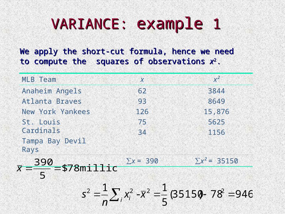
VARIANCE: VARIANCE: example example 11

We apply the short-cut formula, hence we need to We apply the short-cut formula, hence we need to compute the squares of observations compute the squares of observations xx22..

MLB Team x x²


6293

1267534

38448649

15,87656251156

∑x = 390 ∑x² = 35150

millions 78$5

390x

94678)35150(5

1-

1 2222 xx

ns

i i

VARIANCE: VARIANCE: example 2example 2The following data are the 2002 earnings (in thousands of The following data are the 2002 earnings (in thousands of dollars) before taxes for all 6 employees of a small company.dollars) before taxes for all 6 employees of a small company.

48.5048.50 38.4038.40 65.5065.50 22.6022.60 79.8079.80 54.6054.60

x x²

48.5038.4065.5022.6079.8054.60

2352.251474.564290.25510.766368.042981.16

∑x = 309.40 ∑x² = 17977.02

thousands57.51$6

40.309

71.33657.51)02.17977(6

1-

1 2222 ix

n

VARIANCE: frequency distributionVARIANCE: frequency distribution

The formula for variance changes slightly if observations are The formula for variance changes slightly if observations are grouped into a frequency table. Squared deviations are grouped into a frequency table. Squared deviations are multiplied by each frequency's value, and then the total of multiplied by each frequency's value, and then the total of these results is calculated.these results is calculated.

)( 2

2

n

nxi ii


)( 2

2

n

nxxs i ii


222222 -1

and -1

xnxn

snxn i iii ii

The short-cut formulas become:The short-cut formulas become:

VARIANCE: example 3VARIANCE: example 3

Vehicles Owned

(xi)

Number of Households (ni)

xi * ni xi2 xi

2* ni

012345

21811432

01822121210

01491625

01844364850

Sum 40 74 196

85.140

74

n

nxx i ii

48.185.119640

1-

1 2222 xnxn

s ii i

Variance: frequency Variance: frequency distribution with classesdistribution with classes

Again, when the data set is organized in a frequency distribution Again, when the data set is organized in a frequency distribution with classes, we are approximating the data set by "rounding" with classes, we are approximating the data set by "rounding" each value in a given class to the class midpoint. Thus, the each value in a given class to the class midpoint. Thus, the variance of a frequency distribution is given byvariance of a frequency distribution is given by

)( 2

2

n

nm ii i


)( 2

2

n

nxms i ii


where where mmii is the midpoint of each class interval is the midpoint of each class interval.

Short-cut formulasShort-cut formulas

-1 222 ii i nmn

-1 222 xnmn

s ii i

Variance:example 4Variance:example 4The following table gives the frequency distribution of the number of orders The following table gives the frequency distribution of the number of orders

received each day during the past 50 days at the office of a mail-order received each day during the past 50 days at the office of a mail-order company.company.

Number of Orders

Number of Days

nm m2 m*n m2 *n

10 – 1213 – 1516 – 1819 – 21

4122014

11141720

121196289400

44168340280

484235257805600

n= 50 ∑m*n = 832 ∑ m2 *n = 14216

orders. 64.1650

832

n

nmx i ii

43.764.16)14216(50

1-

1 22

i

22 xnmn

s ii

STANDARD DEVIATIONSTANDARD DEVIATION


The The standard deviationstandard deviation is the positive square root of is the positive square root of the variance.the variance.

2

2ss



The standard deviation is the most used measure The standard deviation is the most used measure of dispersion.of dispersion.

The value of the standard deviation tells how The value of the standard deviation tells how closely the values of a data set are clustered closely the values of a data set are clustered around the mean.around the mean.

In general, a lower value of the standard deviation In general, a lower value of the standard deviation for a data set indicates that the values of that data for a data set indicates that the values of that data set are spread over a relatively smaller range set are spread over a relatively smaller range around the mean. around the mean.

In contrast, a large value of the standard deviation In contrast, a large value of the standard deviation for a data set indicates that the values of that data for a data set indicates that the values of that data set are spread over a relatively large range around set are spread over a relatively large range around the mean.the mean.

STANDARD DEVIATIONSTANDARD DEVIATION

STANDARD DEVIATION: STANDARD DEVIATION: example 1example 1

MLB Team

2002 Total Payroll(millions of dollars)

x x²


6293

1267534

38448649

15,87656251156

∑x = 390 ∑x² = 35150

946-1

222 xxn

si i millions 76.30$76.30946 s

millions 78$5

390x

STANDARD DEVIATION: STANDARD DEVIATION: example 2example 2Earnings

(thousands of dollars)

x x²

48.5038.4065.5022.6079.8054.60

2352.251474.564290.25510.766368.042981.16

∑x = 309.40 ∑x² = 17977.02

71.336-1

222 xn

thousands35.18$71.336

thousands57.51$6

40.309

Variance and Standard Deviation: Variance and Standard Deviation: observationsobservations

The values of the variance and the standard The values of the variance and the standard deviation are never negative.deviation are never negative. That is, the That is, the numerator in the formula for the variance should numerator in the formula for the variance should never produce a negative value. Usually the values never produce a negative value. Usually the values of the variance and standard deviation are positive, of the variance and standard deviation are positive, but if data set has no variation, then the variance but if data set has no variation, then the variance and standard deviation are both zero.and standard deviation are both zero.

ExampleExample: 4 persons in a group are the same age – : 4 persons in a group are the same age – say 35 years. If we calculate the variance and the say 35 years. If we calculate the variance and the standard deviation, their values are zero.standard deviation, their values are zero.

CONTINGENCY TABLES CONTINGENCY TABLES AND AND

ELEMENTS OF PROBABILITYELEMENTS OF PROBABILITY

CONTINGENCY TABLES CONTINGENCY TABLES

In many applications the interest is focused on the In many applications the interest is focused on the joint analysis of two variables (qualitative and/or joint analysis of two variables (qualitative and/or quantitative) with the aim of evaluating the relation quantitative) with the aim of evaluating the relation between them.between them.

The variables are usually presented as a The variables are usually presented as a contingency table (contingency table (oror two-way classification two-way classification table).table).

Whereas a frequency distribution provides the Whereas a frequency distribution provides the distribution of one variable, a distribution of one variable, a contingency tablecontingency table describes the distribution of two or more variables describes the distribution of two or more variables simultaneously. simultaneously.


All 420 employees of a company were asked All 420 employees of a company were asked if they are smokers or nonsmokers and if they are smokers or nonsmokers and whether or not they are college graduates.whether or not they are college graduates.

College Graduate

Not a College Graduate

Smoker 35 80

Nonsmoker 130 175

The table gives the distribution of 420 The table gives the distribution of 420 employees based on two variables or employees based on two variables or characters: characters:

XX-smoke -smoke (yes or not) and (yes or not) and YY--graduationgraduation (yes (yes or not)or not)

CellCell

Joint frequency of Joint frequency of category category “Smoker” of X “Smoker” of X and “Not a and “Not a college Graduate” college Graduate” of Yof Y

CONTINGENCY TABLES: CONTINGENCY TABLES: marginal distributions marginal distributions

College Graduat

e

Not a College

GraduateTotal

Smoker 35 80 115

Nonsmoker 130 175 305

Total 165 255 420

The right-hand column and the bottom row are called The right-hand column and the bottom row are called marginal distribution of X marginal distribution of X andand marginal distribution of Y marginal distribution of Y respectivelyrespectively..

Marginal Marginal distribution Ydistribution Y

Marginal Marginal distribution Xdistribution X

XY

Grand Grand TotalTotal


Total

Smoker 115

Nonsmoker 305

420

Total

College graduate

165

Not a College graduate

255

420

%27100*

27.0420

115

115

1010

1010

10

fpn

nf

n

Marginal Marginal distribution Xdistribution X

X Y

Marginal Marginal distribution Ydistribution Y

%39100*

39.0420

165

165

0101

0101

01

fpn

nf

n

CONTINGENCY TABLES: CONTINGENCY TABLES: conditional distributions conditional distributions

College Graduate

Smoker 35

Nonsmoker 130

Total 165

Smoker

College graduate

35

Not a College graduate

80

Total 115

%21

21.0165

35

35

2|11

2|11

11

p

f

n

XY

Conditional distribution Conditional distribution of X to the category of X to the category “College Graduate” of Y“College Graduate” of Y

Conditional distribution of Conditional distribution of Y to the category Y to the category “Smoker” of X“Smoker” of X

XY

%30

30.0115

35

35

1|11

1|11

11

p

f

n NOTE

n

nf

n

nf

n

nf

1111

01

112|11

10

111|11

Definition of probabilityDefinition of probability

There are three different definitions of There are three different definitions of probabilityprobability: : classical definition of probabilityclassical definition of probability, , frequentist definition of probabilityfrequentist definition of probability, , subjective subjective (Bayesian) definition of probability(Bayesian) definition of probability.

Frequentist definition of probability:Frequentist definition of probability:

The relative frequency associated to a category The relative frequency associated to a category of a variable (event) analyzed can be of a variable (event) analyzed can be interpreted as an approximation of the interpreted as an approximation of the probabilityprobability associated to that event. associated to that event.

Definition of probabilityDefinition of probabilityExample: Ten of the 500 randomly selected cars manufactured at a certain auto factory are found to be lemons. Assuming that the lemons are manufactured randomly, what is the probability that the next car manufactured at this auto factory is a lemon?

Car (xi) ni

Relative frequency (fi)

GoodLemon

49010

490/500 = .9810/500 = .02

n = 500

Sum = 1.00

02.500

10lemon) a iscar next ( i

i fn

nP

NOTENOTE:: The relative frequency is an approximation of the The relative frequency is an approximation of the probability!! probability!! Relative frequencies and probabilities get closer as the number Relative frequencies and probabilities get closer as the number of cars increases. of cars increases.

Marginal Probability Marginal Probability

College Graduate

Not a College

GraduateTotal

Smoker 35 80 115


Total 165 255 420

Coming back to the example of the 420 employees. Suppose that one employee is selected at random from the 420 employees. He may be classified on the basis of smoke alone or graduation. The employee can be “smoker”, “nonsmoker”, “graduate”, “nongraduate”.

The probability of each characteristic is called marginal marginal probabilityprobability

Marginal Probability Marginal Probability

College Graduate

Not a College

GraduateTotal

Smoker 35 80 115


Total 165 255 420

61.0420

255)eNonGraduat( 02

02 n

nfP73.0

420

305)Nonsmoker( 20

20 n

nfP

Marginal (Simple) ProbabilityMarginal (Simple) Probability: is the probability (relative frequency) computed on the marginal distributions:

39.0420

165)Graduate( 01

01 n

nfP27.0

420

115)Smoker( 10

10 n

nfP

Joint ProbabilityJoint Probability Suppose that one employees is selected at random from these

420. What is the probability that the employee is a smoker and a College graduate?

College Graduate

Not a College

GraduateTotal

Smoker 35 80 115


Total 165 255 420

It is written as P (Smoker P (Smoker College Graduate).College Graduate). The symbol is read as “and”.

Joint ProbabilityJoint Probability

JointJoint ProbabilityProbability: is the probability (relative frequency) computed on the joint distributions

College Graduate

Not a College

GraduateTotal

Smoker 35 80 115


Total 165 255 420

08.0420

35Graduate) CollegeSmoker( 11

n

nP

Conditional Probability Conditional Probability Now suppose that one employees is selected at random from these 420. Assume that it is known that he is a Smoker. What is the probability that the employee selected is Graduate?

It is written as P P (Graduate|Smoker)(Graduate|Smoker)

It is read as “Probability that he is College Graduate “Probability that he is College Graduate given that he is a Smoker”given that he is a Smoker”

College Graduate

Not a College

GraduateTotal

Smoker 35 80 115


Total 165 255 420

Conditional Probability Conditional Probability

College Graduate

Not a College

GraduateTotal

Smoker 35 80 115


Total 165 255 420

Conditional ProbabilityConditional Probability: is the probability (relative frequency) computed on the conditional distributions:

30.0115

35)mokerGraduate/S(

10

11 n

nP

MEASURES OF DISPERSION. The measures of central tendency, such as the mean, median and mode, do not...

Documents

Transcript of MEASURES OF DISPERSION. The measures of central tendency, such as the mean, median and mode, do not...