
Measures of Central Tendency and LocationMeasures of Central Tendency and Location ... Example 3:...
42
Measures of Central Tendency and Location Copyright by Winston S. Sirug, Ph.D.
Transcript of Measures of Central Tendency and LocationMeasures of Central Tendency and Location ... Example 3:...

Measures of Central
Tendency and
Location
Copyright by Winston S. Sirug, Ph.D.
Measures of Central Tendency
a single value that represents a data set.
Its purpose is to locate the center of a
data set.
commonly referred to as an average.
Properties of Mean
A set of data has only one mean
Applied for interval and ratio data
All values in the data set are included
Very useful in comparing two or more data sets.
Affected by the extreme small or large values on a
data set
Cannot be computed for the data in a frequency
distribution with an open-ended class
Arithmetic Mean (Mean)
The only common measure in which all
values plays an equal role meaning to
determine its values you would need to
consider all the values of any given data
set.
X
mu (for population)μ
X bar (for sample)

Mean for Ungrouped Data
valuesofNumber
valuesallofSumMean
n
XX
N
XPopulation Mean:
Sample Mean:
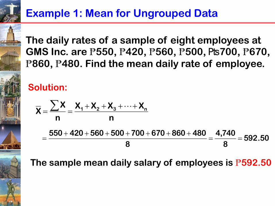
Example 1: Mean for Ungrouped Data
The daily rates of a sample of eight employees at GMS Inc. are ₧550, ₧420, ₧560, ₧500, ₧700, ₧670,
₧860, ₧480. Find the mean daily rate of employee.
n
XXXX
n
XX n321
50.5928
740,4
8
480860670700500560420550
The sample mean daily salary of employees is ₧592.50
Solution:
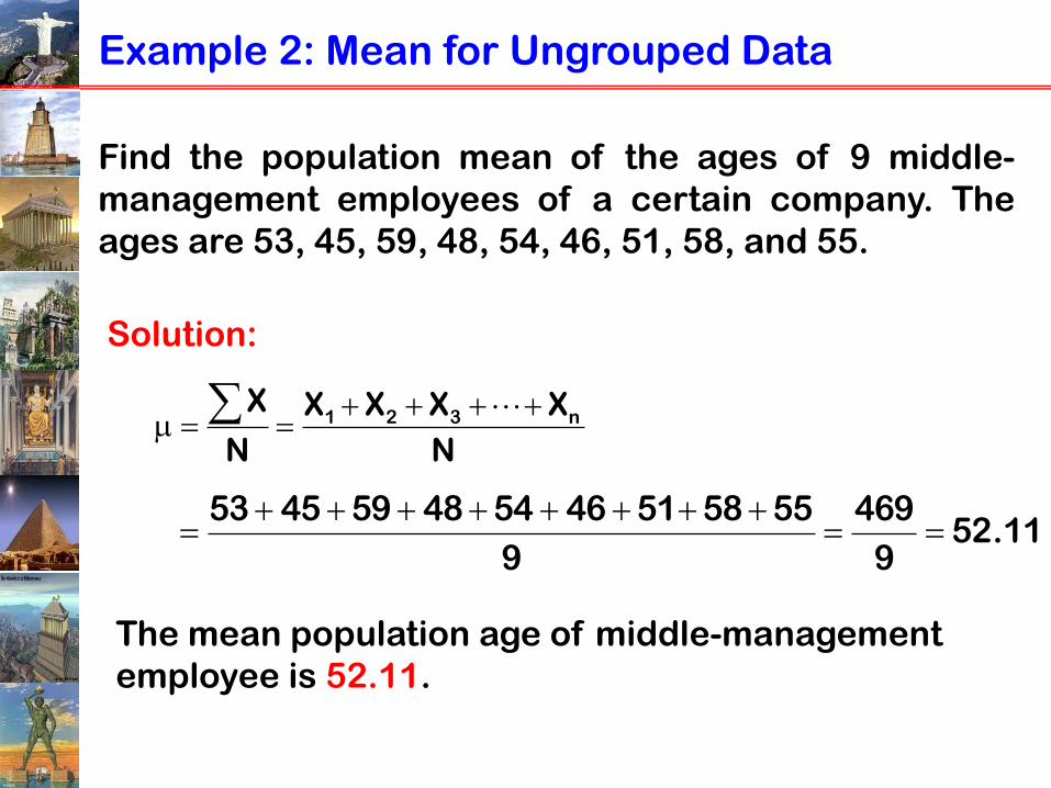
Example 2: Mean for Ungrouped Data
Find the population mean of the ages of 9 middle-
management employees of a certain company. The
ages are 53, 45, 59, 48, 54, 46, 51, 58, and 55.
N
XXXX
N
Xn321
The mean population age of middle-management
employee is 52.11.
Solution:
11.529
469
9
555851465448594553

Mean for Grouped Data
valuesofNumber
valuesallofSumMean
n
fXX
N
fXPopulation Mean:
Sample Mean:
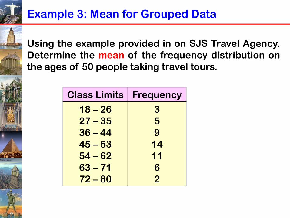
Example 3: Mean for Grouped Data
Using the example provided in on SJS Travel Agency.
Determine the mean of the frequency distribution on
the ages of 50 people taking travel tours.
Class Limits Frequency
18 – 26
27 – 35
36 – 44
45 – 53
54 – 62
63 – 71
72 – 80
3
5
9
14
11
6
2
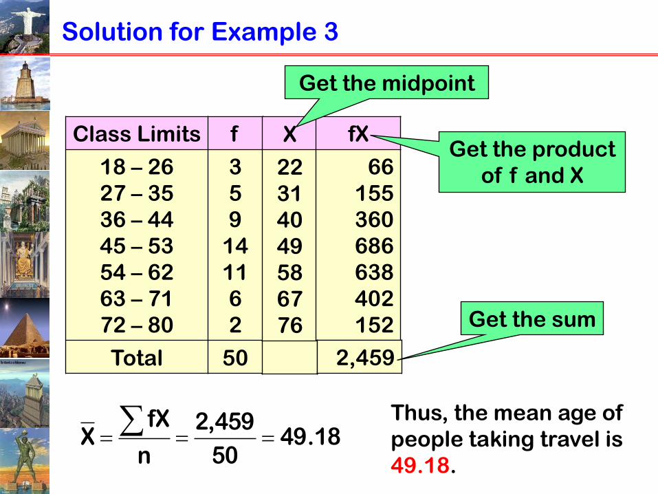
Solution for Example 3
Class Limits f
18 – 26
27 – 35
36 – 44
45 – 53
54 – 62
63 – 71
72 – 80
3
5
9
14
11
6
2
Total 50
X
22
31
40
49
58
67
76
fX
66
155
360
686
638
402
152
Get the midpoint
Get the product
of f and X
2,459
Get the sum
18.4950
459,2
n
fXX
Thus, the mean age of
people taking travel is
49.18.
Median
The midpoint of the data array
Note: Data Array is a data set arranged in
order whether ascending or
descending
Appropriate measure of central tendency
for data that are ordinal or above, but is
more valuable in an ordinal type of data.

Properties of Median
It is unique, there is only one median for a set of
data
It is found by arranging the set of data from lowest
or highest (or highest to lowest) and getting the
value of the middle observation
It is not affected by the extreme small or large
values.
It can be computed for an-open ended frequency
distribution
It can be applied for ordinal, interval and ratio
data
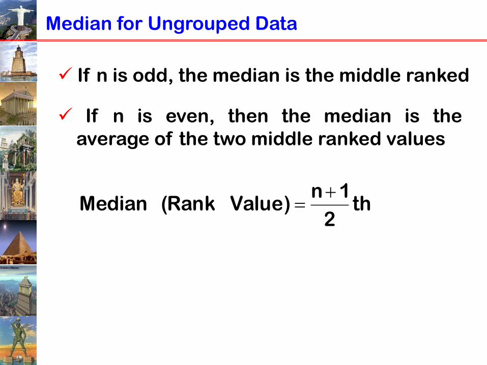
Median for Ungrouped Data
If n is odd, the median is the middle ranked
If n is even, then the median is the
average of the two middle ranked values
th2
1n)ValueRank(Median

Example 1: Median for Ungrouped Data
Find the median of the ages of 9 middle-
management employees of a certain
company. The ages are 53, 45, 59, 48, 54, 46,
51, 58, and 55.
Solution:
45, 46, 48, 51, 53, 54, 55, 58, 59
Step 1: Arranged the data set in order.

Example 1: Median for Ungrouped Data
Step 2: Select the middle rank.
52
10
2
19
2
1n)ValueRank(Median
Step 3: Identify the median in the data set.
45, 46, 48, 51, 53, 54, 55, 58, 59
5th
Hence, the median age is 53 years.
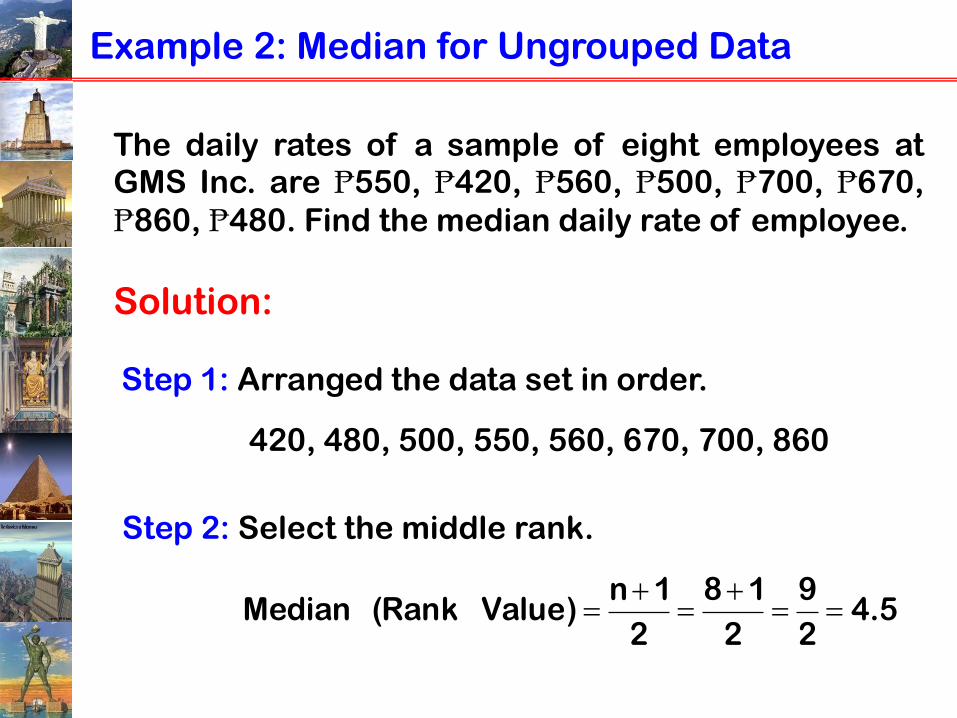
Example 2: Median for Ungrouped Data
The daily rates of a sample of eight employees atGMS Inc. are ₧550, ₧420, ₧560, ₧500, ₧700, ₧670,
₧860, ₧480. Find the median daily rate of employee.
Solution:
420, 480, 500, 550, 560, 670, 700, 860
Step 1: Arranged the data set in order.
5.42
9
2
18
2
1n)ValueRank(Median
Step 2: Select the middle rank.
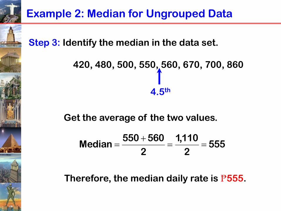
Example 2: Median for Ungrouped Data
Step 3: Identify the median in the data set.
4.5th
Therefore, the median daily rate is ₧555.
420, 480, 500, 550, 560, 670, 700, 860
Get the average of the two values.
5552
110,1
2
560550Median
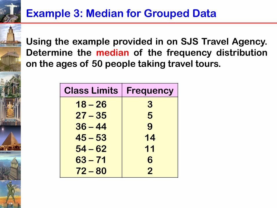
Example 3: Median for Grouped Data
Using the example provided in on SJS Travel Agency.
Determine the median of the frequency distribution
on the ages of 50 people taking travel tours.
Class Limits Frequency
18 – 26
27 – 35
36 – 44
45 – 53
54 – 62
63 – 71
72 – 80
3
5
9
14
11
6
2

Solution for Example 3
Class Limits f
18 – 26
27 – 35
36 – 44
45 – 53
54 – 62
63 – 71
72 – 80
3
5
9
14
11
6
2
Total 50
cf
3
8
17
31
42
48
50
LB = 45 – 0.5
= 44.5
)i(f
cf2
N
LBMedian
64.49)9(14
172
50
5.44
Median Class
cf
f
252
50
2
N)ValueRanked(Median
Median
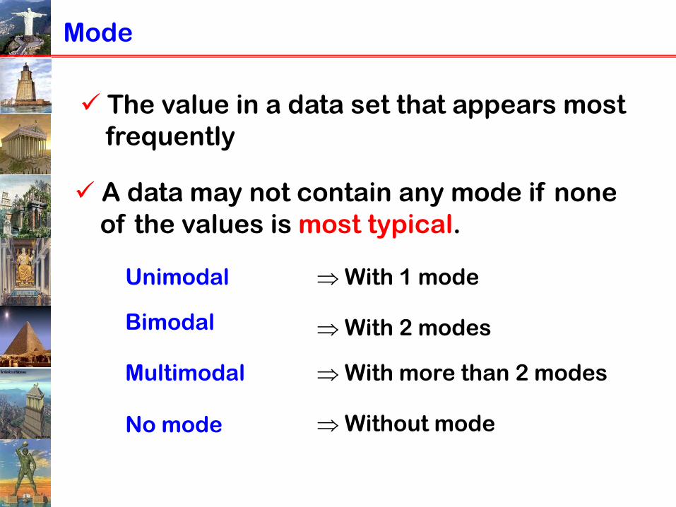
Mode
The value in a data set that appears most
frequently
A data may not contain any mode if none
of the values is most typical.
Unimodal
Bimodal
Multimodal
No mode
With 1 mode
With 2 modes
With more than 2 modes
Without mode

Properties of Mode
It is found by locating the most frequently
occurring value
the easiest average to compute
There can be more than one mode or even no
mode in any given data set
It is not affected by the extreme small or large
values
It can be applied for nominal, ordinal, interval and
ratio data

Example 1: Mode
The following data represent the total sales for PSP
2000 from a sample of 10 Gaming Centers for the
month of August: 15, 17, 10, 12, 13, 10, 14, 10, 8, and 9.
Find the mode.
Therefore the mode is 10.
Solution:
The ordered array for these data is
8, 9, 10, 10, 10, 12, 13, 14, 15, 17
Lowest to Highest

Example 2: Mode
An operations manager in charge of a company’s
manufacturing keeps track of the number of
manufactured LCD television in a day. Compute for the
following data that represents the number of LCD
television manufactured for the past three weeks: 20,
18, 19, 25, 20, 21, 20, 25, 30, 29, 28, 29, 25, 25, 27, 26,
22, and 20. Find the mode of the given data set.
There are two modes 20 and 25.
Solution:
The ordered array for these data is
18, 19, 20, 20, 20, 20, 21, 22, 25, 25, 25, 25, 26, 27, 28,
29, 29, 30
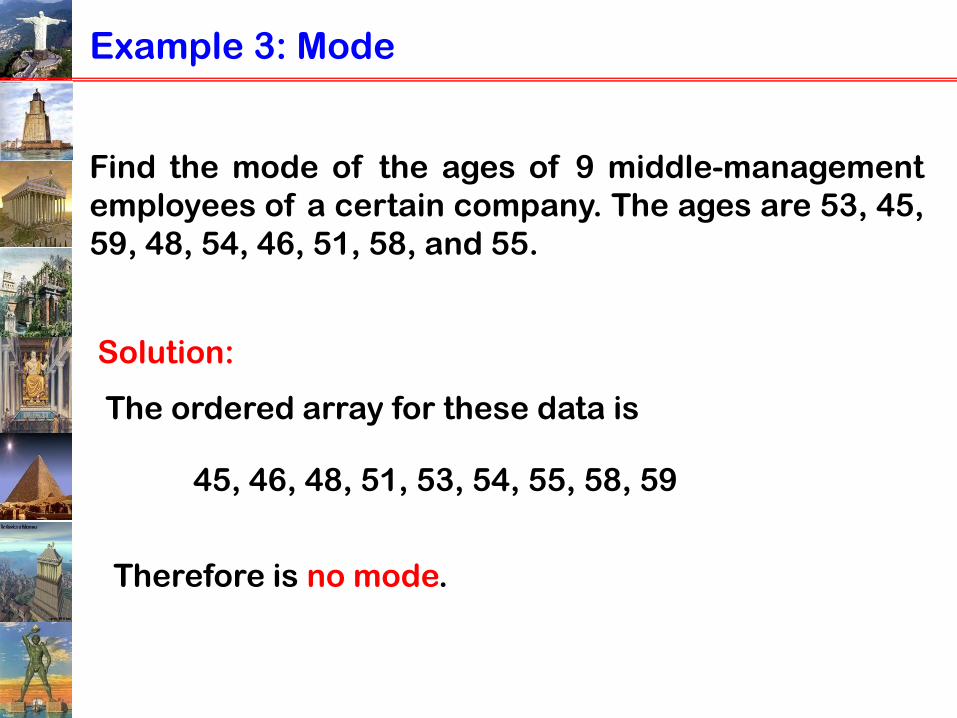
Example 3: Mode
Find the mode of the ages of 9 middle-management
employees of a certain company. The ages are 53, 45,
59, 48, 54, 46, 51, 58, and 55.
Therefore is no mode.
Solution:
The ordered array for these data is
45, 46, 48, 51, 53, 54, 55, 58, 59
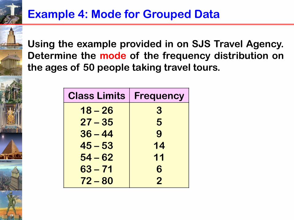
Example 4: Mode for Grouped Data
Using the example provided in on SJS Travel Agency.
Determine the mode of the frequency distribution on
the ages of 50 people taking travel tours.
Class Limits Frequency
18 – 26
27 – 35
36 – 44
45 – 53
54 – 62
63 – 71
72 – 80
3
5
9
14
11
6
2
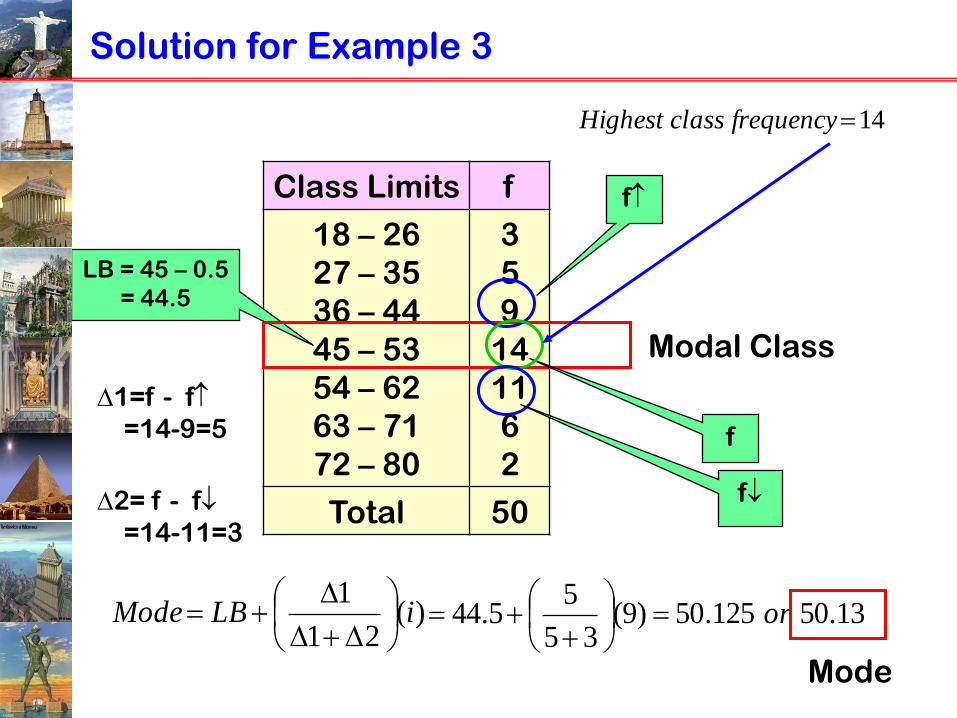
Solution for Example 3
Class Limits f
18 – 26
27 – 35
36 – 44
45 – 53
54 – 62
63 – 71
72 – 80
3
5
9
14
11
6
2
Total 50
LB = 45 – 0.5
= 44.5
)(21
1iLBMode
13.50125.50)9(
35
55.44 or
Modal Class
f
f
14frequencyclassHighest
Mode
f
1=f - f
=14-9=5
2= f - f
=14-11=3
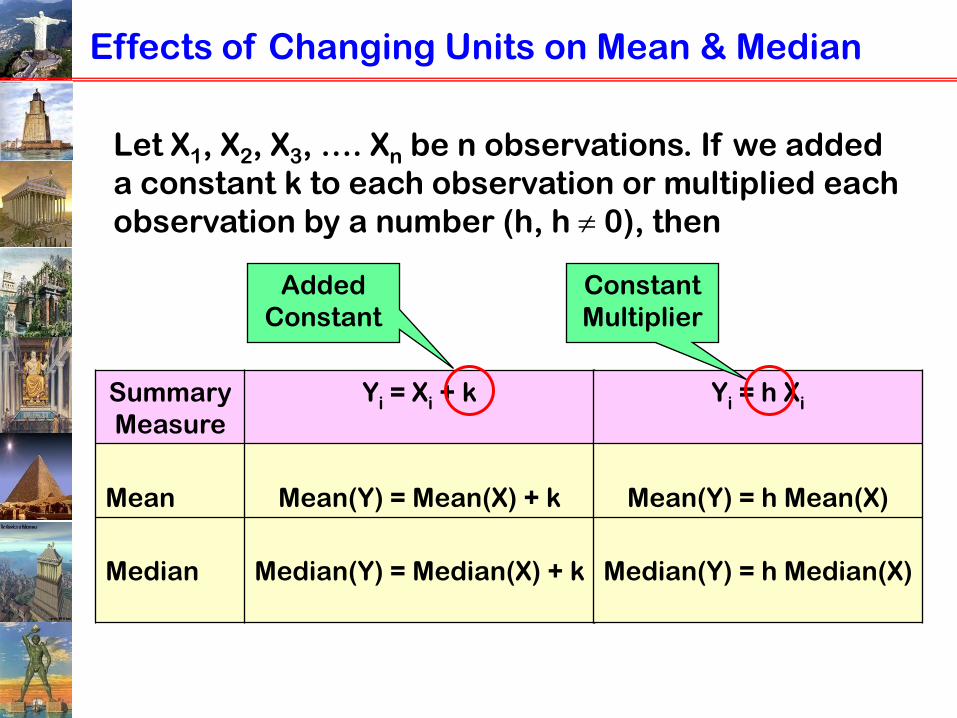
Effects of Changing Units on Mean & Median
Let X1, X2, X3, …. Xn be n observations. If we added
a constant k to each observation or multiplied each
observation by a number (h, h 0), then
Summary
Measure
Yi = Xi + k
Mean Mean(Y) = Mean(X) + k
Median Median(Y) = Median(X) + k
Yi = h Xi
Mean(Y) = h Mean(X)
Median(Y) = h Median(X)
Added
Constant
Constant
Multiplier
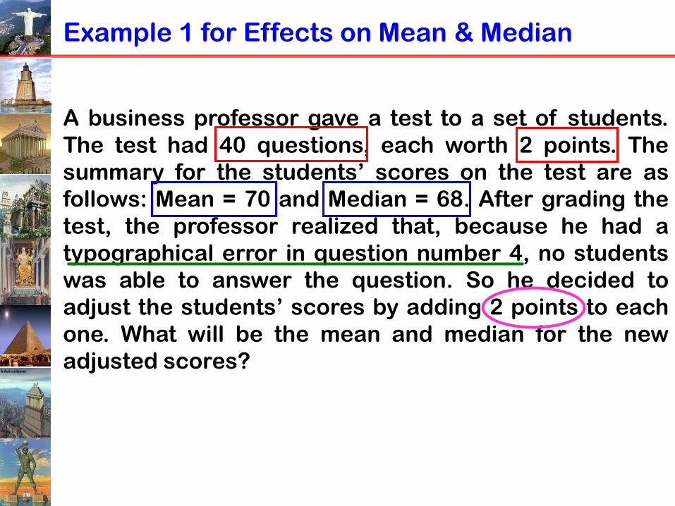
Example 1 for Effects on Mean & Median
A business professor gave a test to a set of students.
The test had 40 questions, each worth 2 points. The
summary for the students’ scores on the test are as
follows: Mean = 70 and Median = 68. After grading the
test, the professor realized that, because he had a
typographical error in question number 4, no students
was able to answer the question. So he decided to
adjust the students’ scores by adding 2 points to each
one. What will be the mean and median for the new
adjusted scores?

Example 1 for Effects on Mean and Median
Solution:
Mean (X) = 70, Median (X) = 68, k = 2
Mean (Y) = Mean (X) + k = 70 + 2 = 72
Median (Y) = Median (X) + k = 68 + 2 = 70
The new mean and median are 72 and 70.
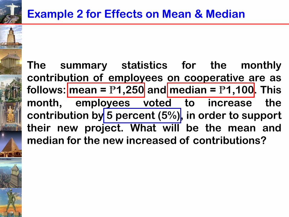
Example 2 for Effects on Mean & Median
The summary statistics for the monthly
contribution of employees on cooperative are asfollows: mean = ₧1,250 and median = ₧1,100. This
month, employees voted to increase the
contribution by 5 percent (5%), in order to support
their new project. What will be the mean and
median for the new increased of contributions?
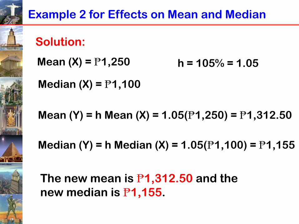
Example 2 for Effects on Mean and Median
Solution:
Mean (X) = ₧1,250
Mean (Y) = h Mean (X) = 1.05(₧1,250) = ₧1,312.50
Median (Y) = h Median (X) = 1.05(₧1,100) = ₧1,155
The new mean is ₧1,312.50 and the
new median is ₧1,155.
h = 105% = 1.05
Median (X) = ₧1,100
OTHER MEASURES OF
LOCATION
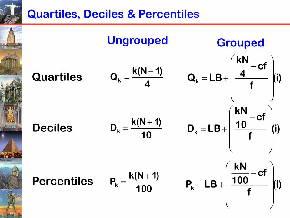
Quartiles, Deciles & Percentiles
Quartiles4
)1N(kQk
Deciles
Percentiles
10
)1N(kDk
100
)1N(kPk
Ungrouped Grouped
)i(f
cf4
kN
LBQk
)i(f
cf10
kN
LBDk
)i(f
cf100
kN
LBPk

Example for Quartiles
Find the 1st, 2nd, and 3rd quartiles of the ages of 9
middle-management employees of a certain
company. The ages are 53, 45, 59, 48, 54, 46, 51, 58,
and 55.
Solution:
4
)1N(1Q1
5.2
4
10
4
)19(1
4
)1N(2Q2
5
4
)10(2
4
)19(2
4
)1N(3Q3
5.7
4
)10(3
4
)19(3
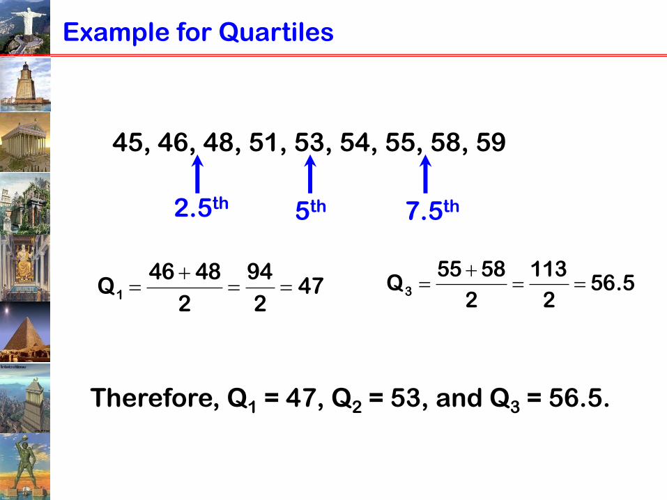
Example for Quartiles
45, 46, 48, 51, 53, 54, 55, 58, 59
2.5th 5th 7.5th
472
94
2
4846Q1
5.56
2
113
2
5855Q3
Therefore, Q1 = 47, Q2 = 53, and Q3 = 56.5.
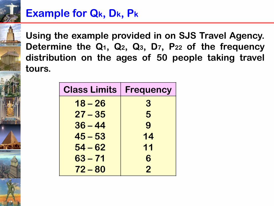
Example for Qk, Dk, Pk
Using the example provided in on SJS Travel Agency.
Determine the Q1, Q2, Q3, D7, P22 of the frequency
distribution on the ages of 50 people taking travel
tours.
Class Limits Frequency
18 – 26
27 – 35
36 – 44
45 – 53
54 – 62
63 – 71
72 – 80
3
5
9
14
11
6
2

Solution for Q1
Class Limits f
18 – 26
27 – 35
36 – 44
45 – 53
54 – 62
63 – 71
72 – 80
3
5
9
14
11
6
2
Total 50
cf
3
8
17
31
42
48
50
LB = 36 –
0.5 = 35.5
)i(f
cf4
N
LBQ1
40)9(9
84
50
5.35
Q1 Class
cf
f
5.124
50
4
N)ValueRanked(Q1
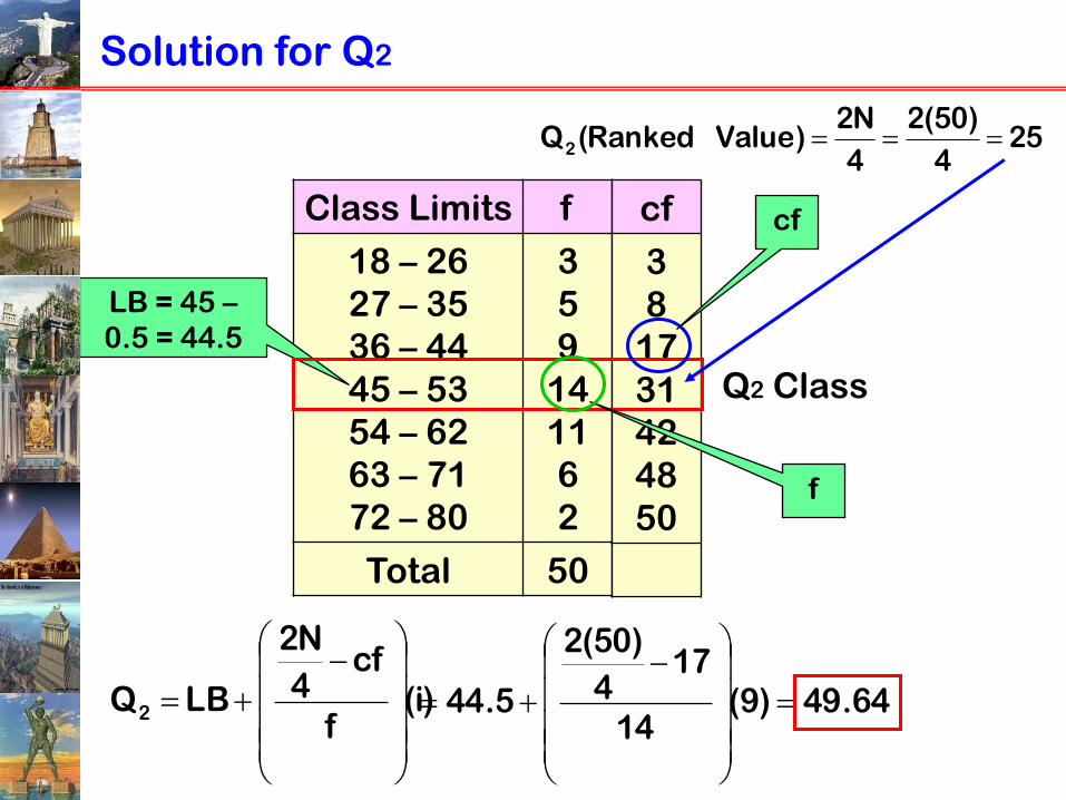
Solution for Q2
Class Limits f
18 – 26
27 – 35
36 – 44
45 – 53
54 – 62
63 – 71
72 – 80
3
5
9
14
11
6
2
Total 50
cf
3
8
17
31
42
48
50
LB = 45 –
0.5 = 44.5
)i(f
cf4
N2
LBQ2
64.49)9(14
174
)50(2
5.44
Q2 Class
cf
f
254
)50(2
4
N2)ValueRanked(Q2
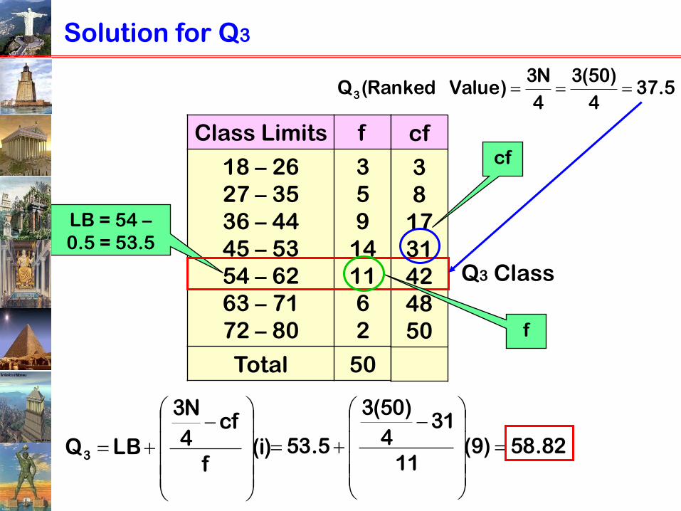
Solution for Q3
Class Limits f
18 – 26
27 – 35
36 – 44
45 – 53
54 – 62
63 – 71
72 – 80
3
5
9
14
11
6
2
Total 50
cf
3
8
17
31
42
48
50
LB = 54 –
0.5 = 53.5
)i(f
cf4
N3
LBQ3
82.58)9(11
314
)50(3
5.53
Q3 Class
cf
f
5.374
)50(3
4
N3)ValueRanked(Q3

Solution for D7
Class Limits f
18 – 26
27 – 35
36 – 44
45 – 53
54 – 62
63 – 71
72 – 80
3
5
9
14
11
6
2
Total 50
cf
3
8
17
31
42
48
50
LB = 54 –
0.5 = 53.5
)i(f
cf10
N7
LBD7
77.56)9(11
3110
)50(7
5.53
D7 Class
cf
f
3510
)50(7
10
N7)ValueRanked(D7

Solution for P22
Class Limits f
18 – 26
27 – 35
36 – 44
45 – 53
54 – 62
63 – 71
72 – 80
3
5
9
14
11
6
2
Total 50
cf
3
8
17
31
42
48
50
LB = 36 –
0.5 = 35.5
)i(f
cf100
N22
LBP22
5.38)9(9
8100
)50(22
5.35
P22 Class
cf
f
11100
)50(22
100
N22)ValueRanked(P22

Whatever exist at all exist in some amount…and
whatever exists in some amount can be
measured.
– Edward L. Thorndike
Copyright by Winston S. Sirug, Ph.D.


