1

Measures of Center

2

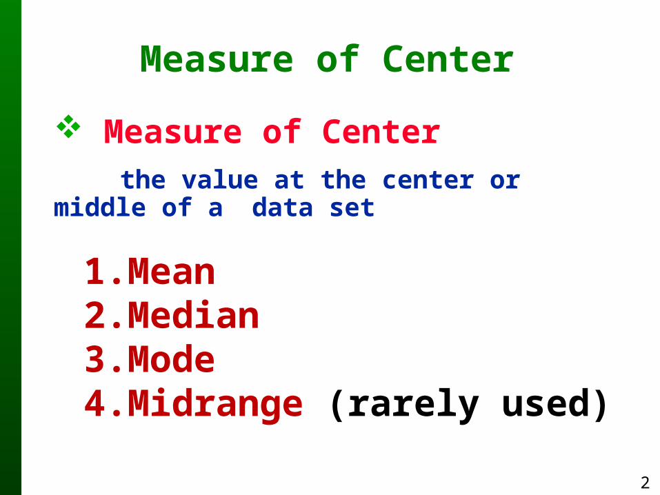
Measure of Center

Measure of Centerthe value at the center or middle of

a data set

1.Mean2.Median3.Mode4.Midrange (rarely used)

3

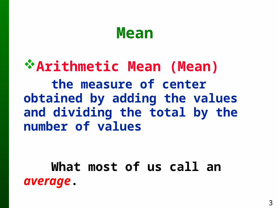
Mean

Arithmetic Mean (Mean)the measure of center obtained by

adding the values and dividing the total by the number of values

What most of us call an average.

4

Notation

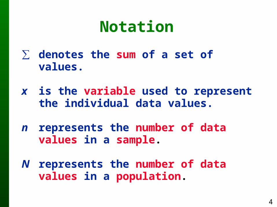
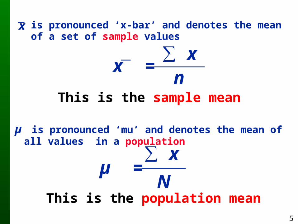
∑ denotes the sum of a set of values.

x is the variable used to represent the individual data values.

n represents the number of data values in a sample.

N represents the number of data values in a population.

5

µ is pronounced ‘mu’ and denotes the mean of all values in a population

x =n∑ x

is pronounced ‘x-bar’ and denotes the mean of a set of sample values

x

Nµ =

∑ x

This is the sample mean

This is the population mean

6

AdvantagesIs relatively reliable.Takes every data value into account

Mean

DisadvantageIs sensitive to every data value, one extreme value can affect it dramatically; is not a resistant measure of center

7

Mean

Example

Major in Geography at University of North Carolina

8

MedianMedian

the middle value when the original data values are arranged in order of increasing (or decreasing) magnitude

often denoted by x (pronounced ‘x-tilde’)~

is not affected by an extreme value - is a resistant measure of the center

9

Finding the Median

1. If the number of data values is odd, the median is the value located in the exact middle of the list.

2. If the number of data values is even, the median is found by computing the mean of the two middle numbers.

First sort the values (arrange them in order), then follow one of these rules:

10

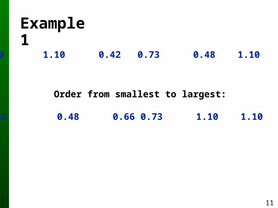
5.40 1.10 0.42 0.73 0.48 1.10 0.66

Example 1

11

5.40 1.10 0.42 0.73 0.48 1.10 0.66

Example 1

0.42 0.48 0.66 0.73 1.10 1.10 5.40

Order from smallest to largest:

12

5.40 1.10 0.42 0.73 0.48 1.10 0.66

Example 1

0.42 0.48 0.66 0.73 1.10 1.10 5.40

Order from smallest to largest:

exact middle MEDIAN is 0.73

13

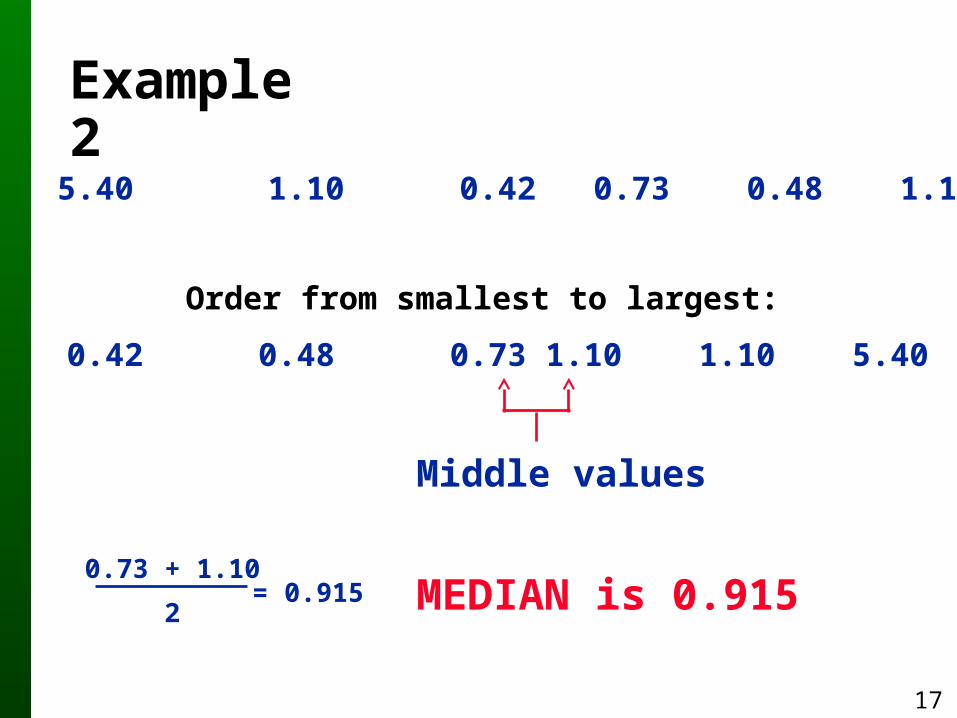
5.40 1.10 0.42 0.73 0.48 1.10

Example 2

14

5.40 1.10 0.42 0.73 0.48 1.10

Example 2

0.42 0.48 0.73 1.10 1.10 5.40

Order from smallest to largest:

15

5.40 1.10 0.42 0.73 0.48 1.10

Example 2

0.42 0.48 0.73 1.10 1.10 5.40

Order from smallest to largest:

Middle values

16

5.40 1.10 0.42 0.73 0.48 1.10

Example 2

0.42 0.48 0.73 1.10 1.10 5.40

Order from smallest to largest:

Middle values

0.73 + 1.10

2= 0.915

17

5.40 1.10 0.42 0.73 0.48 1.10

Example 2

0.42 0.48 0.73 1.10 1.10 5.40

Order from smallest to largest:

Middle values

MEDIAN is 0.9150.73 + 1.10

2= 0.915

18

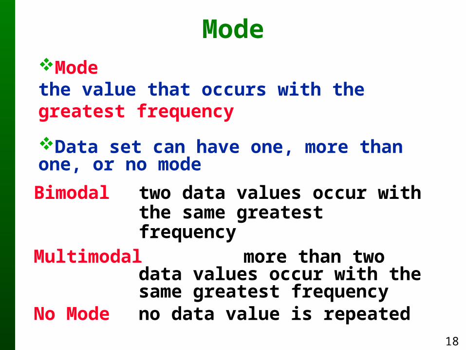
ModeModethe value that occurs with the greatest frequency

Data set can have one, more than one, or no mode

Bimodal two data values occur with the same greatest frequency

Multimodal more than two data values occur with the same greatest frequency

No Mode no data value is repeated

19

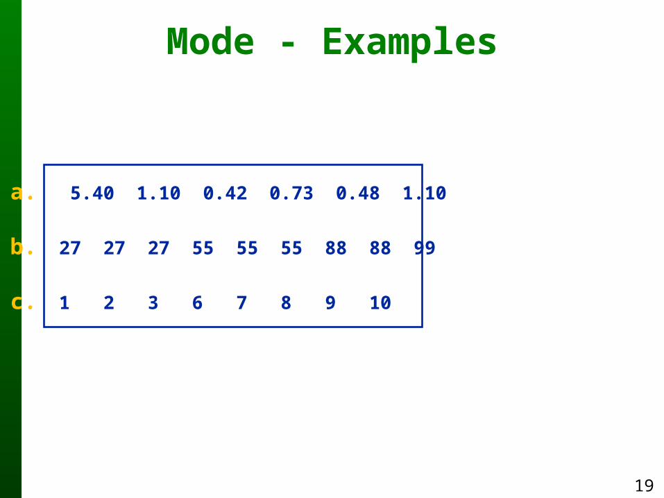
a. 5.40 1.10 0.42 0.73 0.48 1.10

b. 27 27 27 55 55 55 88 88 99

c. 1 2 3 6 7 8 9 10

Mode - Examples

20

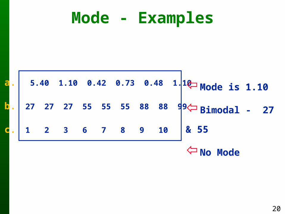
a. 5.40 1.10 0.42 0.73 0.48 1.10

b. 27 27 27 55 55 55 88 88 99

c. 1 2 3 6 7 8 9 10

Mode - Examples

Mode is 1.10

Bimodal - 27 & 55

No Mode

21

Midrange

the value midway between the maximum and minimum values in the original data set

Definition

Midrange =maximum value + minimum value

2

22

Sensitive to extremesbecause it uses only the maximum and minimum values.

Midrange is rarely used in practice

Midrange

23

Carry one more decimal place than is present in the original set of values.

Round-off Rule forMeasures of Center

24

Common Distribution

s

25

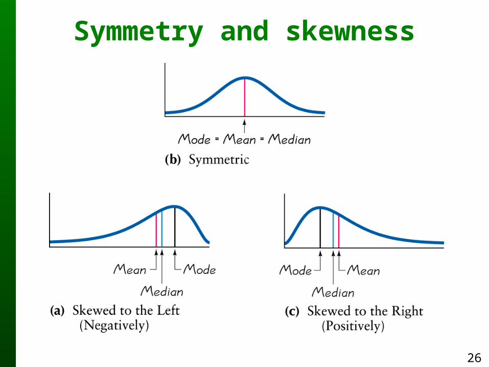
Symmetricdistribution of data is

symmetric if the left half of its histogram is roughly a mirror image of its right half

Skeweddistribution of data is

skewed if it is not symmetric and extends more to one side than the other

Skewed and Symmetric

26

Symmetry and skewness

27

Measures of Variation

28

Measures of Variation

spread, variability of datawidth of a distribution

1.Standard deviation2.Variance3.Range (rarely used)

29

Standard deviation

The standard deviation of a set of sample values, denoted by s, is a measure of variation of values about the mean.

30

Sample Standard Deviation Formula

Σ (x – x)2

n – 1s =

31

Sample Standard Deviation (Shortcut Formula)

n (n – 1)s

=nΣ ( x2) – (Σx)2

32

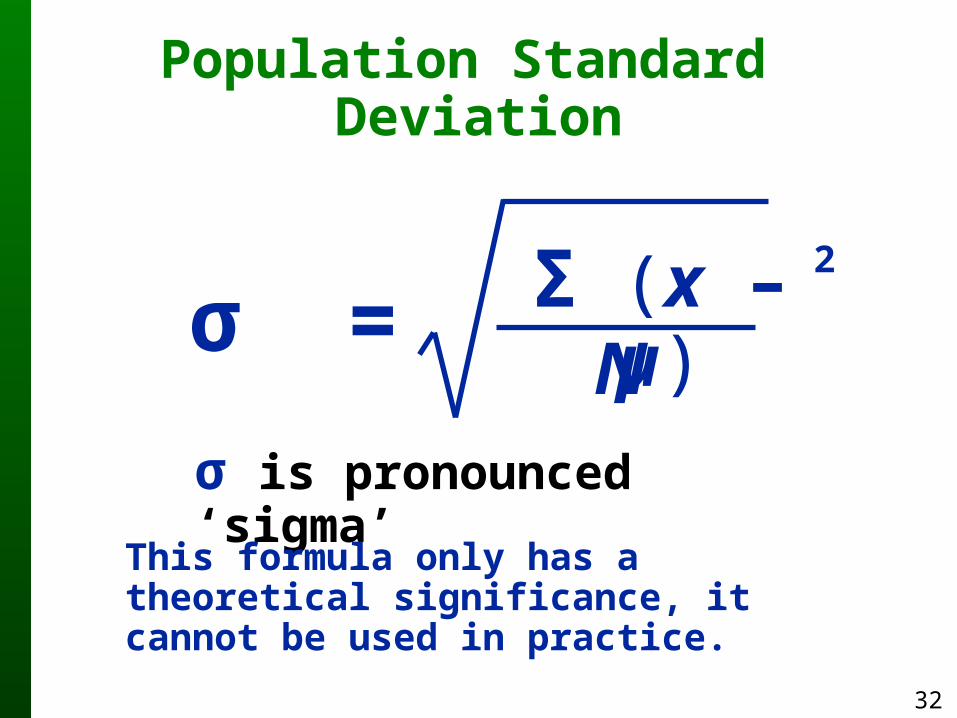
Σ (x – µ)

Population Standard Deviation

2

Nσ =

σ is pronounced ‘sigma’

This formula only has a theoretical significance, it cannot be used in practice.

33

ExampleValues: 1, 3, 14

• Find the sample standard deviation:

• Find the population standard deviation:

34

ExampleValues: 1, 3, 14

• Find the sample standard deviation:

•s = 7.0

• Find the population standard deviation:

•σ = 5.7

35

Population variance: σ2 - Square of the population standard deviation σ

Variance

The variance is a measure of variation equal to the square of the standard deviation.

Sample variance: s2 - Square of the sample standard deviation s

36

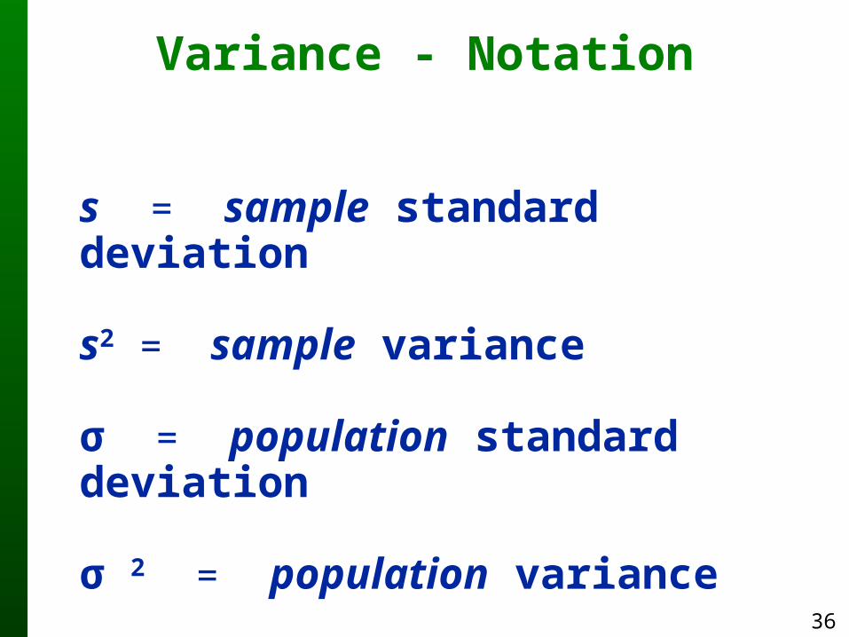
Variance - Notation

s = sample standard deviation

s2 = sample variance

σ = population standard deviation

σ 2 = population variance

37

ExampleValues: 1, 3, 14

s = 7.0

s2 = 49.0

σ = 5.7

σ2 = 32.7

38

Range(Rarely used)

The difference between the maximum data value and the minimum data value.

Range = (maximum value) – (minimum value)

It is very sensitive to extreme values; therefore range is not as useful as the other measures of variation.

39

Using Excel

40

Using Excel

Enter values into first column

41

Using Excel

In C1, type “=average(a1:a6)”

42

Using Excel

Then, Enter

43

Using Excel

Same thing with “=stdev(a1:a6)”

44

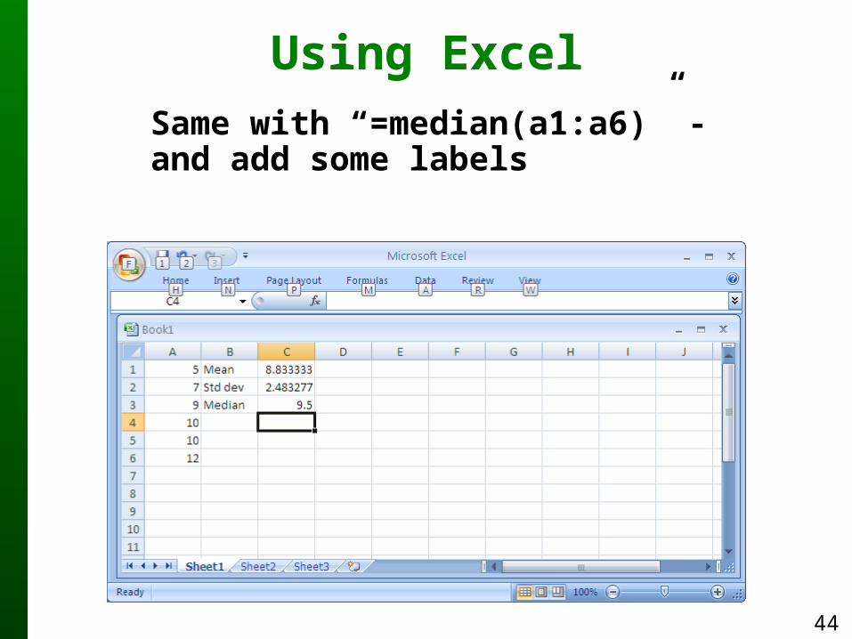
Using ExcelSame with “=median(a1:a6)” - and add some labels

45

Using Excel

Same with min, max, and mode

46

Usual and Unusual Events

47

Usual values in a data set are those that are typical and not too extreme.

Minimum usual value =

(mean) – 2 * (standard deviation)

Maximum usual value =

(mean) + 2 * (standard deviation)

48

Usual values in a data set are those that are typical and not too extreme.

sxxsx 22

49

Rule of Thumb

Based on the principle that for many data sets, the vast majority (such as 95%) of sample values lie within two standard deviations of the mean. A value is unusual if it differs from the mean by more than two standard deviations.

50

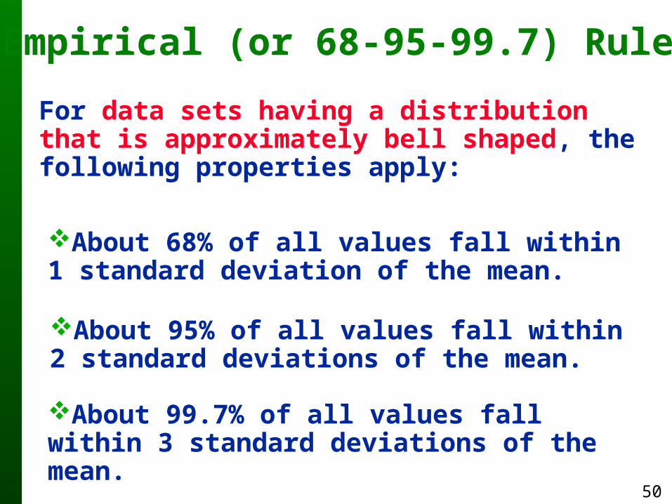
Empirical (or 68-95-99.7) Rule

For data sets having a distribution that is approximately bell shaped, the following properties apply:

About 68% of all values fall within 1 standard deviation of the mean.

About 95% of all values fall within 2 standard deviations of the mean.

About 99.7% of all values fall within 3 standard deviations of the mean.

51

The Empirical Rule

52

The Empirical Rule

53

The Empirical Rule

54

Measures of Relative Standing

55

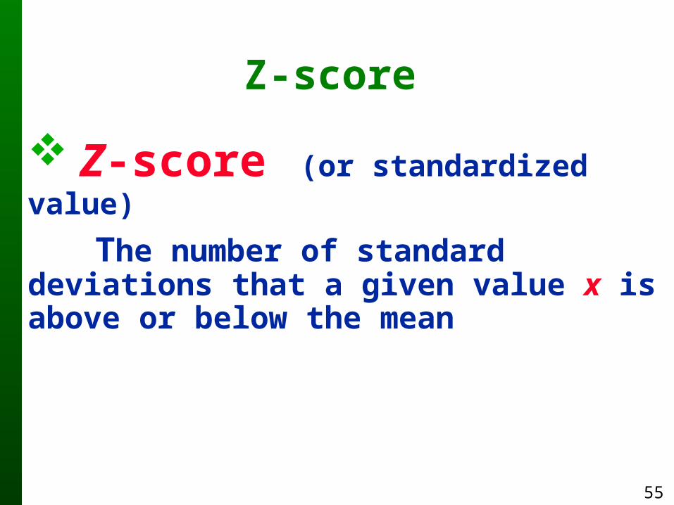
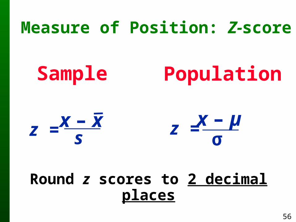
Z-score (or standardized value)

The number of standard deviations that a given value x is above or below the mean

Z-score

56

Sample Population

x – µz =σ

Round z scores to 2 decimal places

Measure of Position: Z-score

z =x – xs

57

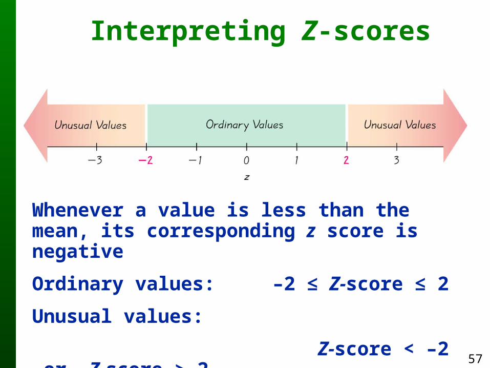
Interpreting Z-scores

Whenever a value is less than the mean, its corresponding z score is negative

Ordinary values: –2 ≤ Z-score ≤ 2

Unusual values:

Z-score < –2 or Z-score > 2

58

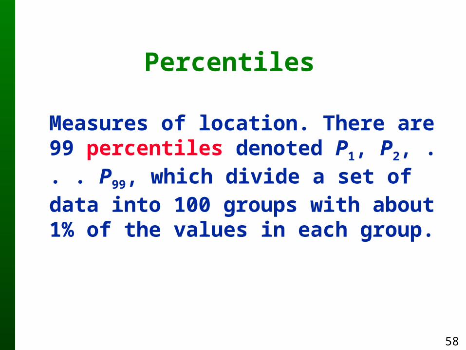
Percentiles

Measures of location. There are 99 percentiles denoted P1, P2, . . . P99, which divide a set of data into 100 groups with about 1% of the values in each group.

59

Finding the Percentileof a Data Value

Percentile of value x = • 100number of values less than x

total number of values

Round it off to the nearest whole number

60

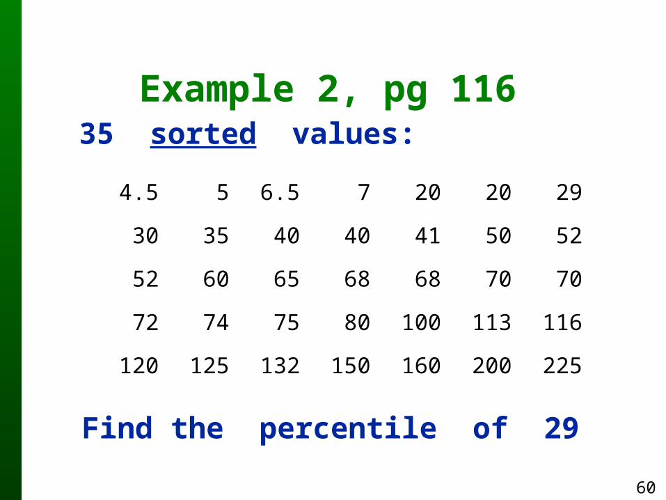
Example 2, pg 11635 sorted values:

Find the percentile of 29

4.5 5 6.5 7 20 20 29

30 35 40 40 41 50 52

52 60 65 68 68 70 70

72 74 75 80 100 113 116

120 125 132 150 160 200 225

61

Example 2, pg 11635 sorted values:

Find the percentile of 29

Percentile of 29 = 17 (rounded)

4.5 5 6.5 7 20 20 29

30 35 40 40 41 50 52

52 60 65 68 68 70 70

72 74 75 80 100 113 116

120 125 132 150 160 200 225

62

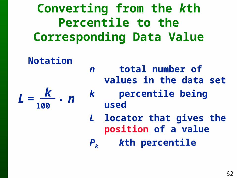
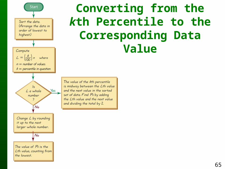
n total number of values in the data set

k percentile being usedL locator that gives the

position of a valuePk kth percentile

L = • nk100

Notation

Converting from the kth Percentile to the Corresponding

Data Value

63

Example 3, pg 11635 sorted values:

Find P60

4.5 5 6.5 7 20 20 29

30 35 40 40 41 50 52

52 60 65 68 68 70 70

72 74 75 80 100 113 116

120 125 132 150 160 200 225

64

Example 3, pg 11635 sorted values:

Find P60

P60 = 71

4.5 5 6.5 7 20 20 29

30 35 40 40 41 50 52

52 60 65 68 68 70 70

72 74 75 80 100 113 116

120 125 132 150 160 200 225

65

Converting from thekth Percentile to theCorresponding Data

Value

66

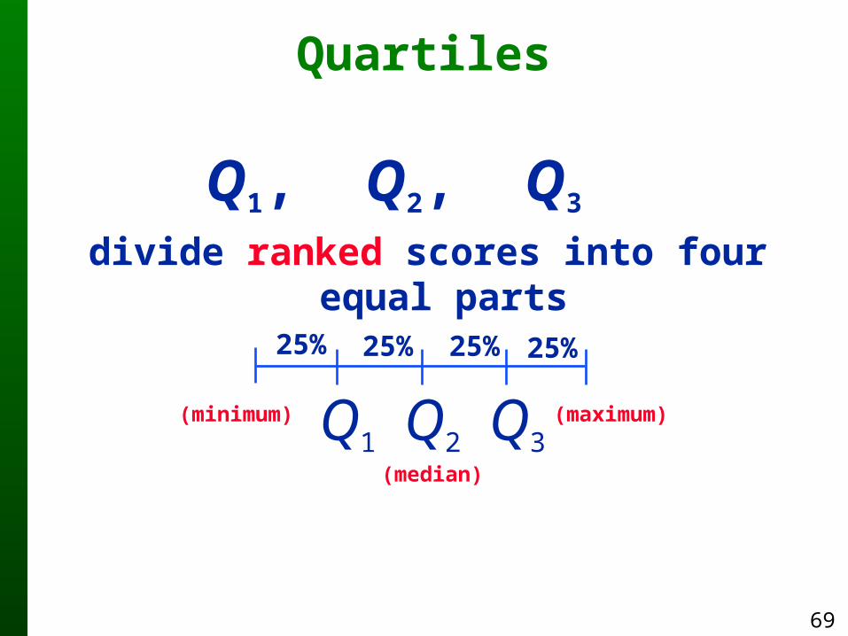
Quartiles

Q1 (First Quartile) separates the bottom 25% of sorted values from the top 75%.

Q2 (Second Quartile) same as the median; separates the bottom 50% of sorted values from the top 50%.

Q3 (Third Quartile) separates the bottom 75% of sorted values from the top 25%.

Measures of location, denoted Q1, Q2, and Q3, which divide a set of data into four groups with about 25% of the values in each group.

67

Quartiles

To calculate the quartile for homework and other CourseCompass work, using Excel:

1.Sort the data

2.Enter =quartile(<range>,1)

3.Find the result in the sorted data

4.If the result is not in the sorted data, go to the next higher value

68

Example - Quartile

=quartile(A1:G5,1) give 37.537.5 is between 35 and 40The 1st quartile value is 40

4.5 5 6.5 7 20 20 29

30 35 40 40 41 50 52

52 60 65 68 68 70 70

72 74 75 80 100 113 116

120 125 132 150 160 200 225

69

Q1, Q2, Q3 divide ranked scores into four equal

parts

Quartiles

25% 25% 25% 25%

Q3Q2Q1(minimum) (maximum)

(median)

70

Interquartile Range (or IQR): Q3 – Q1

10 - 90 Percentile Range: P90 – P10

Semi-interquartile Range:2

Q3 – Q1

Midquartile:2

Q3 + Q1

Some Other Statistics

71

For a set of data, the 5-number summary consists of the● minimum value

●first quartile Q1

●median (or second quartile Q2)

●third quartile, Q3

●maximum value.

5-Number Summary

72

Example35 sorted values:

Find the 5-number summary

4.5 5 6.5 7 20 20 29

30 35 40 40 41 50 52

52 60 65 68 68 70 70

72 74 75 80 100 113 116

120 125 132 150 160 200 225

73

Example

Min = 4.5Q1 = 40Median = 50Q3 = 1130Max = 225