Measurements of Electron Density Profiles Using an · PDF filebe made using shadowgraph and...

MeasureMents of electron Density Profiles using an angular filter refractoMeter

LLE Review, Volume 13750

IntroductionAn understanding of the underdense plasma conditions in laser–plasma experiments at large laser facilities is important for many high-energy-density (HED) physics studies.1 The growth of laser–plasma instabilities depends on the coronal plasma density profile, flow, and temperature. When they are above threshold, they can feed back onto the hydrodynamics often requiring ad hoc modeling of the laser absorption or heat transport.2 In high-temperature plasmas, the primary instabili-ties of interest are stimulated Brillouin scattering,3 stimulated Raman scattering,3 and two-plasmon decay.4

Quantitative characterization of HED plasma density profiles in the corona where the laser–plasma interactions are most active is challenging. Incoherent x-ray sources are useful for diagnos-ing cold (Te # 10 eV) and dense (ne . 1023 cm–3) plasmas, where absorption and scattering techniques such as radiography/pen-umbral imaging5 and x-ray Thomson scattering6 are employed. Optical wavelengths are typically employed to probe lower-density ranges where the plasma density is inferred from the phase change of the probe beam. These diagnostics are designed to access the plasma density by measuring the probe beam’s phase (interferometry7), refraction angle (schlieren imaging,8 grid image refractometry,9 and Moire deflectometry10), or displacement (shadowgraphy8). In the range of densities above 1020 cm–3, typical HED plasmas present large integrated optical phases that make it difficult to quantitatively measure the density profile. Soft x-ray lasers present an alternative to access these density ranges,11 but are a complex radiation source and often not practical for application to large-scale diagnostic systems.

A qualitative picture of the underdense plasma gradients can be made using shadowgraph and schlieren imaging, although these techniques are not precise enough to extract the plasma density profile.8 In shadowgraphy, the displacement of probe rays is mapped by imaging a plane behind the object in ques-tion. An image is recorded not of the object, but of its shadow, which does not have a 1:1 spatial correspondence with the object. Extracting the plasma density would involve decon-volving the spatial correspondence, calculating the absorption

Measurements of Electron Density Profiles Using an Angular Filter Refractometer

profile of the probe beam, and a double integration to achieve the probe’s phase. This typically introduces an unacceptable amount of error into the density measurement. Schlieren techniques map the refraction of the probe beam by blocking all or part of the unrefracted probe beam with a knife edge or a circular stop. In the case of using a coherent probe pulse produced by a laser, only a single refraction angle is measured, lending this technique to be used for the observation of sharp density gradients such as in the presence of a shock,12 where the binary response of the diagnostic is useful. Extracting quantita-tive information from the density gradients with a significant dynamic range involves the use of an incoherent probe pulse such as a light-emitting diode with an extended source size.13

Interferometry is the most-common technique used for measuring plasma density profiles in underdense plasmas. As the probe passes through higher-density regions of the plasma, the interferometric fringes become closer and are eventually unresolvable. It is difficult to quantify this limita-tion in resolution, but for a particular profile, synthetic inter-ferograms can be generated to study the peak plasma density that can be resolved using interferometry. Taking a typical HED laser–plasma plume from a planar target modeled as

exp expn n x y L z L02 2 2

e g n- -= +_ _i i8 B with Lg = 400 nm and Ln = 300 nm, the maximum peak density resolvable with a 263-nm probe on a standard detector is +1020 cm–3, which is consistent with the peak densities measured by D. Ress et al.14 for a comparable-sized plasma.

Angular filter refractometry (AFR),15,16—a novel diagnos-tic—has been developed to characterize the plasma density profile up to densities of 1021 cm–3 by producing a contour map of refraction angles. This is accomplished by using angular filters that block certain bands of refraction angles, casting shadows in the image plane. The plasma density is calculated from the measured refraction angles of a probe beam after passing through the plasma. The maximum measured density is limited by the f number of the optical collection system, the length of plasma in the direction of the probe, and the mag-nitude of the transverse gradients. AFR provides an accurate


LLE Review, Volume 137 51

diagnosis of the underdense plasma profiles in experiments relevant to laser–plasma instabilities.

The following sections (1) describe the operation of the AFR diagnostic and how the experimental images can be analyzed to produce two-dimensional (2-D) plasma density profiles; (2) review experiments in which the diagnostic was used to characterize the plasma expansion from ultraviolet irradiated CH planar and spherical targets; and (3) present the conclu-sions. The error analysis of the AFR diagnostic is presented in the Appendix.

Angular Filter RefractometryThe AFR diagnostic is a part of the fourth-harmonic probe

system17 on OMEGA EP.18 A simplified optical schematic of the system is shown in Fig. 137.42. The red lines represent the incoming ray path of the probe beam. It originates from the conversion of a Nd:glass laser pulse to its fourth harmonic (probe wavelength mp = 263 nm) and has a pulse width of 10 ps with 10 mJ of energy. The beam passes through the target chamber center (TCC) slightly diverging at f/25 with a beam diameter of +3.5 mm. After passing through the TCC, the probe is collected at f/4 and collimated for transport over >4 m to the diagnostic table, where the plasma plane is relay imaged to a charge-coupled–device (CCD) camera with a resolution of +5 nm over a 5-mm field of view.15

1. Diagnostic Setup and CalibrationThe AFR diagnostic uses an angular filter [Fig. 137.43(a)]

placed at the focus of the unrefracted probe beam (Fourier plane19). The opaque regions of the angular filter block bands of refraction angles, resulting in shadows in the image plane. The diagnostic relies on the direct proportionality between the angle of refraction of a probe ray at the object plane and its radial location in the Fourier plane. This relation correlates the shadows produced by the angular filter to contours of the constant refraction angle. For a single-lens imaging system and a collimated probe beam, it can be shown that a ray refracted at the object plane passes through the Fourier plane at a distance from the optical axis r, which is equal to the focal length of the collection lens f, times the refraction angle i, regardless of its spatial origin in the object plane [assuming paraxial propaga-tion cos(i) . 1] (Ref. 20). For the case of a diverging probe beam (used in the AFR diagnostic), a more-general relation is determined using geometric optics where r is equal to a con-stant times the refraction angle iref, according to

,rd d f

d f

1ref

s

s#

-i= +

f p (1)

where iref = itot–i0, itot is the ray angle with respect to the optical axis, i0 is the initial unrefracted angle, d1 is the dis-

E22424JR

Objectplane(TCC)

Collectionlens

85 cmds

1.2 md1

4.6 m1.1 m 0.7 m

Collimationlens

Imaginglens

Fourierplane

Angular�lter

Imageplane

itot

i0 r

ˆ

ˆˆ

y

zx

Figure 137.42A schematic representation of angular filter refractometry using the fourth-harmonic probe on OMEGA EP (distances not to scale). The unrefracted probe (red) focuses at the Fourier plane, where distinct refraction angles are filtered out by an angular filter. Shadows from the opaque regions of the angular filter form contours of constant refraction angle in the image plane. TCC: target chamber center.



tance from the object plane to the collection lens, and ds is the distance from the point source to the object plane (ds = 3 for the collimated beam). The direct proportionality of the spatial location of a ray to the amount of refraction allows for filtration of specific refraction angles in a deterministic manner.

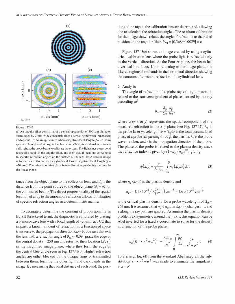
To accurately determine the constant of proportionality in Eq. (1) (bracketed term), the diagnostic is calibrated by placing a planoconcave lens with a focal length of –20 mm at TCC that imparts a known amount of refraction as a function of space transverse to the propagation direction (x,y). Probe rays that exit the lens with a refraction angle of iref = 0.09° graze the edge of the central dot at r = 250 nm and return to their location ,x yl l_ i in the magnified image plane, where they form the edge of the central blue circle seen in Fig. 137.43(b). Higher refraction angles are either blocked by the opaque rings or transmitted between them, forming the other light and dark bands in the image. By measuring the radial distance of each band, the posi-

tions of the rays at the calibration lens are determined, allowing one to calculate the refraction angles. The resultant calibration for the image shown relates the angle of refraction to the radial position on the angular filter, iref = [0.368!0.0029] # r.

Figure 137.43(c) shows an image created by using a cylin-drical calibration lens where the probe light is refracted only in the vertical direction. At the Fourier plane, the beam has a vertical line focus. Upon returning to the image plane, the filtered regions form bands in the horizontal direction showing the contours of constant refraction of a cylindrical lens.

2. AnalysisThe angle of refraction of a probe ray exiting a plasma is

related to the transverse gradient of phase accrued by that ray according to7

,2p

2

2i

r

m

a

z=a (2)

where a (= x or y) represents the spatial component of the measured refraction in the x–y plane (see Fig. 137.42), mp is the probe laser wavelength, z = #kpdz is the total accumulated phase of a probe ray passing through the plasma, kp is the probe wave number, and z is the propagation direction of the probe. The phase of the probe is related to the plasma density since the refractive index is given by /1 2,n n1 e cr-_ i giving

, , , ,x yn

n x y z zdp cr

ezmr

=-3

3

a ak k# (3)

where ne (x,y,z) is the plasma density and

. .n 1 1 10 1 6 10m cm cm21 2 3 22 3cr p# #m n= =- -a k

is the critical plasma density for a probe wavelength of mp = 263 nm. It is assumed that ne % ncr. In Eq. (3), changes in x and y along the ray path are ignored. Assuming the plasma density profile is axisymmetric around the y axis, this equation can be Abel inverted for a fixed y coordinate to solve for the density as a function of the probe phase:

.n R x zn

x s R

sd2 22 2 2

0

ep cr

-2

2

r

m z= + =

+

-3

'` j (4)

To arrive at Eq. (4) from the standard Abel integral, the sub-stitution s x R2 2-= was made to eliminate the singularity at x = R.

E22425JR

–1

–1

0

1

0

(b) (c)

(a)

x axis (mm)

y ax

is (

mm

)

1 –1 0

x axis (mm)

1

Figure 137.43(a) An angular filter consisting of a central opaque dot of 500-nm diameter surrounded by 2-mm-wide concentric rings alternating between transparent and opaque. (b) An image formed when a negative-focal-length ( f = –20 mm) spherical lens placed at target chamber center (TCC) is used to deterministi-cally refract the probe beam to calibrate the system. The light rings correspond to specific bands in the angular filter, and their spatial locations correspond to specific refraction angles on the surface of the lens. (c) A similar image is formed as in (b) but with a cylindrical lens of negative focal length ( f = –20 mm). The refraction takes place in one direction, producing the lines in the image plane.



For the circular angular filter shown in Fig. 137.43(a), the total refraction angle is measured, .x y

2 2toti i i= + Owing to

the shape of the plasmas expanding from the flat and spherical targets studied here, the direction of the refraction is assumed to be radial; therefore, Eq. (2) is integrated in the radial direction about the assumed center of the plasma to solve for the phase of the probe beam exiting the plasma. The gradient of the phase in the x direction (perpendicular to the axis of symmetry) is used to solve for the plasma density using Eq. (4). An error analysis of the data reduction and calibration is presented in Appendix A (p. 56).

To reduce the numerical error introduced by calculating the gradient in phase, an angular filter with straight lines parallel to the y axis can be used to directly determine the component of the refraction in the x direction (2z/2x). In this case the measured refraction angle (ix) can be directly inserted into Eq. (4) so that both the integration in Eq. (2) and the derivative in Eq. (4) are skipped.

Experimental ResultsThe plasma density profiles for flat and spherical plastic CH

targets driven by four ultraviolet laser beams (m0 = 351 nm) incident at an angle of 23° with respect to the target normal were measured. Each beam had +2 kJ of energy in a 2-ns square temporal pulse shape. Distributed phase plates21 were used to produce a 9.5-order super-Gaussian spot with 430-nm (1/e) width on the target surface, resulting in a total peak overlapped intensity of 8 # 1014 W/cm2. The fourth-harmonic probe pulse passed transverse to the target normal. The short probe pulse’s duration of 10 ps ensures that there is minimal hydrodynamic movement of the plasma over the course of the measurement. The timing of the probe is defined from the 2% intensity of the ultraviolet drive beams to the peak intensity of the probe.

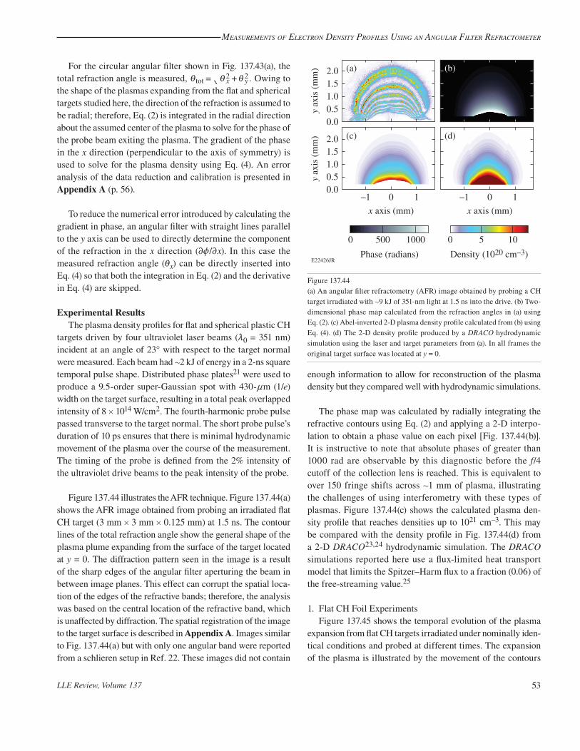
Figure 137.44 illustrates the AFR technique. Figure 137.44(a) shows the AFR image obtained from probing an irradiated flat CH target (3 mm # 3 mm # 0.125 mm) at 1.5 ns. The contour lines of the total refraction angle show the general shape of the plasma plume expanding from the surface of the target located at y = 0. The diffraction pattern seen in the image is a result of the sharp edges of the angular filter aperturing the beam in between image planes. This effect can corrupt the spatial loca-tion of the edges of the refractive bands; therefore, the analysis was based on the central location of the refractive band, which is unaffected by diffraction. The spatial registration of the image to the target surface is described in Appendix A. Images similar to Fig. 137.44(a) but with only one angular band were reported from a schlieren setup in Ref. 22. These images did not contain

enough information to allow for reconstruction of the plasma density but they compared well with hydrodynamic simulations.

The phase map was calculated by radially integrating the refractive contours using Eq. (2) and applying a 2-D interpo-lation to obtain a phase value on each pixel [Fig. 137.44(b)]. It is instructive to note that absolute phases of greater than 1000 rad are observable by this diagnostic before the f/4 cutoff of the collection lens is reached. This is equivalent to over 150 fringe shifts across +1 mm of plasma, illustrating the challenges of using interferometry with these types of plasmas. Figure 137.44(c) shows the calculated plasma den-sity profile that reaches densities up to 1021 cm–3. This may be compared with the density profile in Fig. 137.44(d) from a 2-D DRACO23,24 hydrodynamic simulation. The DRACO simulations reported here use a flux-limited heat transport model that limits the Spitzer–Harm flux to a fraction (0.06) of the free-streaming value.25

1. Flat CH Foil ExperimentsFigure 137.45 shows the temporal evolution of the plasma

expansion from flat CH targets irradiated under nominally iden-tical conditions and probed at different times. The expansion of the plasma is illustrated by the movement of the contours

E22426JR

0.00.51.01.52.0

y ax

is (

mm

)

–10.00.51.01.52.0

0

x axis (mm)

y ax

is (

mm

)

1

Density (1020 cm–3)

0 5 10

(c)

–1 0

x axis (mm)

1

(d)

(b)(a)

Phase (radians)

0 500 1000

Figure 137.44(a) An angular filter refractometry (AFR) image obtained by probing a CH target irradiated with +9 kJ of 351-nm light at 1.5 ns into the drive. (b) Two-dimensional phase map calculated from the refraction angles in (a) using Eq. (2). (c) Abel-inverted 2-D plasma density profile calculated from (b) using Eq. (4). (d) The 2-D density profile produced by a DRACO hydrodynamic simulation using the laser and target parameters from (a). In all frames the original target surface was located at y = 0.



in the radial direction away from the target surface (y = 0). Figure 137.45(d) is from the same shot as Fig. 137.44(a). An estimate of the plasma expansion is obtained by assuming a 2-D Gaussian-shaped plasma in the target plane direction and an exponential profile in the target normal direction of the form ne(y) = n0 exp(–y/Ln), where Ln is the plasma scale length. Taking two points in the center of the profile at x = 0, Eqs. (2) and (3) can be used to show .lnL y y1 2 2 1n - i i= a `k j Fol-

lowing two points of constant refraction yields the proportional-ity Ln ? y1–y2. As time increases, the widening and separating of the refractive bands signify a proportionate increase in the plasma scale length as the plasma expands away from the target.

Figure 137.46 shows 1-D density profiles along the y axis obtained from the experimental images shown in Fig. 137.45. Density data are extracted over almost two orders of mag-

E22081JR

0.0–0.50.0

0.5

1.0

1.5

2.0

0.5

x axis (mm)

y ax

is (

mm

)

0.0–0.5 0.5

x axis (mm)

0.0–0.5 0.5

x axis (mm)

0.0–0.5 0.5

x axis (mm)

0.0–0.5 0.5

x axis (mm)

(a) (b) (c) (d) (e)

Figure 137.45Central portions of AFR images illustrating plasma expansion from flat CH targets irradiated with +9 kJ of ultraviolet (351-nm) light in a 1-mm spot. The images were obtained at probe timings of (a) 0.56 ns, (b) 0.84 ns, (c) 1.1 ns, (d) 1.5 ns, and (e) 2.0 ns.

E22363aJR

0.5 1.0

(b)(a)

y axis (mm)

1.5 2.00.5 1.0

y axis (mm)

1.5 2.0

1019

1020

1021

Plas

ma

dens

ity (

cm–3

)

1.5-ns experiment1.5-ns simulation2.0-ns experiment2.0-ns simulation

Error in density Error in density

0.56-ns experiment0.56-ns simulation0.84-ns experiment0.84-ns simulation1.1-ns experiment1.1-ns simulation

Figure 137.46Plasma density profiles along the target normal at the center of the plasma profile (x = 0) obtained from the AFR images of Fig. 137.45 (solid lines). The shaded regions represent DRACO simulations covering a time span of 40 ps, corresponding to the ! error in measuring the probe-pulse timing with respect to the ultraviolet drive pulses. The original target position is located at y = 0. The error bars on the experimental data represent !15% as derived in Appendix A (p. 56).



nitude ranging from +3 # 1019 to 1021 cm–3. The upper end is limited by refraction of the probe beam outside of the f/4 collection optics, and the lower end is limited by the smallest measurable refraction angle by this angular filter (0.21°). The profiles are approximately exponential,26 and for the early times (#1.1 ns) shown in Fig. 137.46(a), the plasma expands away from the surface driven by the ablation. This is evident in the increase in the position for a given value of density as time increases. The expansion ceases at later times ($1.5 ns) shown in Fig. 137.46(b) except at the low-density region of the profile. The shaded regions in Fig. 137.46 represent lineouts from the DRACO-simulated plasma profiles, where the width of the shaded region accounts for the !20-ps timing error in the probe pulse. The experimental data agree very well with the simulations for early times (<1 ns). For times $1.1 ns, the simulations predict higher plasma densities than are experi-mentally measured. This can also be seen from a comparison between Figs. 137.44(c) and 137.44(d).

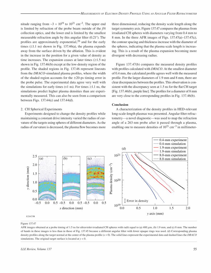
2. CH Spherical ExperimentsExperiments designed to change the density profiles while

maintaining a constant drive intensity varied the radius of cur-vature of the targets using spheres of different diameters. As the radius of curvature is decreased, the plasma flow becomes more

three dimensional, reducing the density scale length along the target symmetry axis. Figure 137.47 compares the plasmas from irradiated CH spheres with diameters varying from 0.4 mm to 8 mm. In the three AFR images of Figs. 137.47(a)–137.47(c), the contour spacing and thickness increase with the diameter of the spheres, indicating that the plasma scale length is increas-ing. This is a result of the plasma expansion becoming more divergent with decreasing radius.

Figure 137.47(b) compares the measured density profiles with profiles calculated with DRACO. At the smallest diameter of 0.4 mm, the calculated profile agrees well with the measured profile. For the larger diameters of 1.9 mm and 8 mm, there are clear discrepancies between the profiles. This observation is con-sistent with the discrepancy seen at 1.5 ns for the flat CH target [Fig. 137.46(b), purple line]. The profiles for a diameter of 8 mm are very close to the corresponding profiles in Fig. 137.46(b).

ConclusionA characterization of the density profiles in HED-relevant

long-scale-length plasmas was presented. Angular filter refrac-tometry—a novel diagnostic—was used to map the refraction angle of a 263-nm probe after it passed through a plasma, enabling one to measure densities of 1021 cm–3 in millimeter-

E22427JR

–0.5 0.0

(a) (b) (c)

0.0

0.5

1.0

1.5

2.0

2.5

0.5 –0.5 0.0

x direction (mm)

y di

rect

ion

(mm

)

0.5 –0.5 0.0 0.5

(d)

0.0

1021

1020

1019

Plas

ma

dens

ity (

cm–3

)

0.5 1.0 1.5 2.0

y axis (mm)

0.4-mm experiment0.4-mm simulation1.9-mm experiment1.9-mm simulation8.0-mm experiment8.0-mm simulation

Error in density

Figure 137.47AFR images obtained at a probe timing of 1.5 ns for ultraviolet-irradiated CH spheres with radii equal to (a) 400 nm, (b) 1.9 mm, and (c) 8 mm. The number of bands in these images is less than in those of Fig. 137.45 because a different angular filter with fewer opaque rings was used. (d) Corresponding plasma density profiles along the target normal at the center of the plasma profile (x = 0). The solid lines represent the experimental data and dashed lines the DRACO simulations. The original target surface is located at y = 0.



scale plasmas. The plasma expansion from kilojoule-level, ultraviolet-irradiated CH targets was studied as a function of time for planar targets and radius for spherical targets. These results were compared with 2-D DRACO hydrodynamic simu-lations showing good agreement for the planar targets at early times and for the spherical targets at small radii. The hydro-dynamic simulations predict higher densities for the planar targets at late times and for the spherical targets with larger radii. The difference between the experimental and simulation data is under active investigation and focused on correlations to laser–plasma instabilities that could possibly modify the plasma profile at large scale lengths.

ACKNOWLEDGMENTThis material is based upon work supported by the Department of

Energy National Nuclear Security Administration under Award Number DE-NA0001944, the University of Rochester, and the New York State Energy Research and Development Authority. The support of DOE does not constitute an endorsement by DOE of the views expressed in this article.

Appendix A: Error AnalysisThe calibration of refraction angles and the post-analysis

process are the two significant sources of error in the calcula-tion of plasma density from the AFR images. To estimate the error in the calibration process, the system was calibrated four times over a two-month period to take into account the reproducibility of the lens placement at TCC and the accuracy of marking the edges of the refractive bands. For each calibra-tion, a constant of proportionality relating the refraction angle iref to the radial location on the angular filter r was calculated. The standard deviation in that constant was found to be v = 0.0029°/mm. This error was propagated through the analysis process and yielded a corresponding standard deviation error in the plasma density of 2%.

The reduction of an experimental AFR image to a plasma density profile includes many steps: locating the refraction bands, radially integrating the refraction angle to produce a phase, and Abel inverting the phase to produce plasma den-sity. There is an error in the optical imaging system caused by the continuous refraction by an extended plasma around the object plane. It is difficult to estimate the contribution of each of these effects to the error. The error was therefore extracted by analyzing a synthetic AFR image created by an optical model. The optical ray-trace code FRED27 was used to assess the performance of the optical probe system and data-reduction method. FRED is a nonsequential ray-trace package that pro-vides synthetic probe images for an assumed plasma density

profile. The full diagnostic system was simulated in FRED. An analytic plasma density profile was used in the optical model to create a synthetic AFR image. This image was post-processed and the resulting plasma density profile was compared to the original to extract the error. The standard deviation of the error in a pixel-by-pixel comparison of the two profiles was 12.2%. Adding this to the error in calibration gives a total error in the plasma density calculation of !14.2%.

It is important to register the AFR images with respect to the original position of the target surface, especially for comparing to hydrodynamic simulations. For this purpose a background shot (without the drive beams) is taken to produce a shadow of the target onto the CCD by removing the angular filter. The front surface of the target is determined by measur-ing the position of an alignment fiber (80-nm diameter) that is attached to the middle of the flat target on the rear surface. In this manner, any diffculty in clearly observing the front surface, which extends about a millimeter beyond the object plane, is mitigated. The fiber tip resides at TCC and is imaged sharply. With prior knowledge of the separation between the fiber tip and the front surface of the target, the position of the original surface is accurately determined within !10 nm, near the resolution limit of the diagnostic. For spherical targets, the surface is sharply imaged and therefore directly observed without a fiducial.

The timing of the optical probe is measured with respect to the ultraviolet drive laser beams by comparison to a timing fiducial used to synchronize all laser beams on OMEGA EP. A small portion of each beam is picked off upstream of TCC and measured on a UV streak camera to compare to the fiducial on shot. The absolute calibration of the distance between these timing diagnostic signals and TCC is measured periodically with a time-resolved x-ray target diagnostic, also referenced to the facility timing fiducial. Multiple calibrations measured over several months have shown a scattering of !20 ps. This error is taken into account when comparing to DRACO simulations by using two time steps and shading the area between t0–20 ps and t0 + 20 ps, where t0 is the measured experimental timing of the optical probe.

REFERENCES

1. National Research Council (U.S.) Committee on High Energy Den-sity Plasma Physics, Frontiers in High Energy Density Physics: The X-Games of Contemporary Science (The National Academies Press, Washington, DC, 2003).

2. P. Michel et al., Phys. Plasmas 20, 056308 (2013).



3. W. L. Kruer, in The Physics of Laser Plasma Interactions, Frontiers in Physics, Vol. 73, edited by D. Pines (Westview Press, Boulder, CO, 2003).

4. M. V. Goldman, Ann. Phys. 38, 117 (1966).

5. S. Fujioka et al., Rev. Sci. Instrum. 73, 2588 (2002).

6. S. H. Glenzer, G. Gregori, F. J. Rogers, D. H. Froula, S. W. Pollaine, R. S. Wallace, and O. L. Landen, Phys. Plasmas 10, 2433 (2003).

7. I. H. Hutchinson, Principles of Plasma Diagnostics, 2nd ed. (Cam-bridge University Press, Cambridge, England, 2002).

8. G. S. Settles, Schlieren and Shadowgraph Techniques: Visualizing Phenomena in Transparent Media (Springer, Berlin, 2001).

9. R. S. Craxton, F. S. Turner, R. Hoefen, C. Darrow, E. F. Gabl, and Gar. E. Busch, Phys. Fluids B 5, 4419 (1993).

10. J. Ruiz-Camacho, F. N. Beg, and P. Lee, J. Phys. D: Appl. Phys. 40, 2026 (2007).

11. D. Ress et al., Science 265, 514 (1994).

12. M. T. Carnell and D. C. Emmony, Opt. Laser Technol. 26, 385 (1994).

13. D. Estruch et al., Rev. Sci. Instrum. 79, 126108 (2008).

14. D. Ress et al., Phys. Fluids B 2, 2448 (1990).

15. D. Haberberger, S. Ivancic, M. Barczys, R. Boni, and D. H. Froula, in CLEO: Applications and Technology, CLEO 2013: Technical Digest (Optical Society of America, Washington, DC, 2013), Paper ATu3M.3.

16. U. Kogelschatz and W. R. Schneider, Appl. Opt. 11, 1822 (1972).

17. D. H. Froula, R. Boni, M. Bedzyk, R. S. Craxton, F. Ehrne, S. Ivancic, R. Jungquist, M. J. Shoup, W. Theobald, D. Weiner, N. L. Kugland, and M. C. Rushford, Rev. Sci. Instrum. 83, 10E523 (2012).

18. J. H. Kelly, L. J. Waxer, V. Bagnoud, I. A. Begishev, J. Bromage, B. E. Kruschwitz, T. J. Kessler, S. J. Loucks, D. N. Maywar, R. L. McCrory, D. D. Meyerhofer, S. F. B. Morse, J. B. Oliver, A. L. Rigatti, A. W. Schmid, C. Stoeckl, S. Dalton, L. Folnsbee, M. J. Guardalben, R. Jungquist, J. Puth, M. J. Shoup III, D. Weiner, and J. D. Zuegel, J. Phys. IV France 133, 75 (2006).

19. J. W. Goodman, Introduction to Fourier Optics, 3rd ed. (Roberts and Company Publishers, Englewood, CO, 2005).

20. J. T. Verdeyen, Laser Electronics, 3rd ed. (Prentice-Hall, Englewood Cliffs, NJ, 1995).

21. T. J. Kessler, Y. Lin, J. J. Armstrong, and B. Velazquez, in Laser Coher-ence Control: Technology and Applications, edited by H. T. Powell and T. J. Kessler (SPIE, Bellingham, WA, 1993), Vol. 1870, pp. 95–104.

22. W. Seka, R. S. Craxton, R. E. Bahr, D. L. Brown, D. K. Bradley, P. A. Jaanimagi, B. Yaakobi, and R. Epstein, Phys. Fluids B 4, 432 (1992).

23. D. Keller, T. J. B. Collins, J. A. Delettrez, P. W. McKenty, P. B. Radha, B. Whitney, and G. A. Moses, Bull. Am. Phys. Soc. 44, 37 (1999).

24. P. B. Radha, T. J. B. Collins, J. A. Delettrez, Y. Elbaz, R. Epstein, V. Yu. Glebov, V. N. Goncharov, R. L. Keck, J. P. Knauer, J. A. Marozas, F. J. Marshall, R. L. McCrory, P. W. McKenty, D. D. Meyerhofer, S. P. Regan, T. C. Sangster, W. Seka, D. Shvarts, S. Skupsky, Y. Srebro, and C. Stoeckl, Phys. Plasmas 12, 056307 (2005).

25. R. C. Malone, R. L. McCrory, and R. L. Morse, Phys. Rev. Lett. 34, 721 (1975).

26. S. Atzeni and J. Meyer-ter-Vehn, The Physics of Inertial Fusion: Beam Plasma Interaction, Hydrodynamics, Hot Dense Matter, International Series of Monographs on Physics (Clarendon Press, Oxford, 2004).

27. Photon Engineering, LLC, Tucson, AZ 85711.

Measurements of Electron Density Profiles Using an · PDF filebe made using shadowgraph and...

Documents

Transcript of Measurements of Electron Density Profiles Using an · PDF filebe made using shadowgraph and...