MEASUREMENT OF WALL RELAXATION TIMES OF POLARIZED 3HE IN BULK LIQUID 4HE FOR THE NEUTRON ELECTRIC DIPOLE MOMENT EXPERIMENT

BY

JACOB YODER

DISSERTATION

Submitted in partial fulfillment of the requirements for the degree of Doctor of Philosophy in Physics

in the Graduate College of the University of Illinois at Urbana-Champaign, 2010

Urbana, Illinois

Doctoral Committee:

Professor Jen-Chieh Peng, Chair Professor Douglas H. Beck, Director of Research Professor Steven M. Errede Professor Michael Stone

ii

Abstract

The Neutron Electric Dipole Moment (nEDM) experiment that will take place at

the Spallation Neutron Source (SNS) in Oak Ridge, Tennessee will measure the electric

dipole moment (EDM) of the neutron with a precision of order 10-28 e-cm, utilizing spin-

polarized 3He in bulk liquid 4He to detect neutron precession in a 10 mG magnetic field

and 50 kV/cm electric field. Since depolarized 3He will produce a background,

relaxation of the polarized 3He, characterized by the probability of depolarization per

bounce, Pd, was measured for materials that will be in contact with polarized 3He.

Depolarization probabilities were determined from measurements of the

longitudinal relaxation time of polarized 3He in bulk liquid 4He inside an acrylic cell

coated with the wavelength shifter deuterated tetraphenyl butadiene (d-TPB), which

will be used to coat the nEDM measurement cell. Relaxation measurements were also

performed while rods, made from plumbing material Torlon and valve bellows material

BeCu, were present in the cell. The BeCu was coated with Pyralin resin prior to

relaxation measurements, while relaxation measurements were performed both before

and after the Torlon rod was coated with Pyralin resin. The depolarization probabilities

were found to be

<d-TPB 7

Bare Torlon 6

Coated Torlon 7

Coated BeCu 7

1.32 10

1.01 0.08 10

2.5 0.1 10

7.9 0.3 10

d

d

d

d

P

P

P

P

The relaxation rates extrapolated from the observed values of Pd for d-TPB,

coated Torlon, and coated BeCu in the nEDM apparatus were found to be consistent

with design goals.

iii

Table of Contents List of Figures ....................................................................................................v List of Tables ....................................................................................................ix 1 Introduction..............................................................................................1

1.1 Symmetries and CP Violation............................................................................... 2 1.1.1 Weak Sector CP Violation in Neutral Kaon Decay....................................... 2 1.1.2 The BAU........................................................................................................ 3 1.1.3 Strong CP violation in the MSM................................................................... 6 1.1.4 Modifications to the Minimal Standard Model (MSM) ................................. 6 1.1.5 Using the Neutron EDM to Measure CP Violation ....................................... 7 1.1.6 History of Neutron EDM Searches................................................................. 9

1.2 The Proposed Measurement at SNS.................................................................... 12 1.2.1 UCN Production ...........................................................................................13 1.2.2 Neutron Precession Measurement .................................................................15

1.3 3He Relaxation..................................................................................................... 17 1.3.1 Long Range Magnetic Gradients ..................................................................18 1.3.2 Wall Relaxation ............................................................................................20 1.3.3 Wall Materials ..............................................................................................22 1.3.4 Small Scale Materials Test............................................................................23

2 Method ...................................................................................................25 2.1 Design Requirements ........................................................................................... 25 2.2 Polarized 3He Production .................................................................................... 27

2.2.1 Optical Pumping...........................................................................................27 2.2.2 3He Gas System for the OPC........................................................................29

2.3 Refrigeration........................................................................................................ 31 2.4 Measurement Cell................................................................................................ 35 2.5 B0 Magnet and Field Uniformity......................................................................... 38 2.6 Magnetometry in the Measurement Cell ............................................................. 44 2.7 Procedures ........................................................................................................... 46

2.7.1 Pre-Cooldown Preparations ..........................................................................46 2.7.2 77 K Procedures............................................................................................47 2.7.3 Relaxation Measurements Below 4.2 K ........................................................50

3 Results ...................................................................................................54 3.1 Raw Data ............................................................................................................ 54 3.2 FID Curve Fits.................................................................................................... 56 3.3 T1 Fit Technique ................................................................................................. 59

3.3.1 Thermal Settling ...........................................................................................60 3.3.2 Liquid 4He Volume........................................................................................62 3.3.3 Diffusion Effects............................................................................................63

3.4 T1 Fit Results ...................................................................................................... 66 3.4.1 Empty Cell....................................................................................................66 3.4.2 Bare Torlon Sample Rod ..............................................................................69 3.4.3 Coated Torlon Rod .......................................................................................70 3.4.4 Coated BeCu Rod .........................................................................................72

3.5 Depolarization Probabilities ................................................................................ 73 4 Conclusions.............................................................................................75

4.1 Wall Relaxation in nEDM................................................................................... 75 4.2 Concentration and Temperature Effects ............................................................. 77 4.3 Future Work........................................................................................................ 78

A B1 Coil Calibration................................................................................80 B 3He Transport Simulation.......................................................................83

iv

References ...................................................................................................87

v

List of Figures Figure 1.1: Plot of primordial light nuclei abundances versus baryon asymmetry parameter. Gray regions show estimates of primordial abundances. Systematic errors in the estimates of abundances are not known, particularly with 7Li and D+3He. D+3He was once thought to be constant, but 3He is destroyed within stars to some degree, making D+3He difficult to estimate. .................................................................................................. 4

Figure 1.2: a) The parity transformation reverses the EDM direction but leaves the spin unchanged. b) Time reversal changes the direction of the spin but leaves the EDM unchanged. ....................................................................... 8

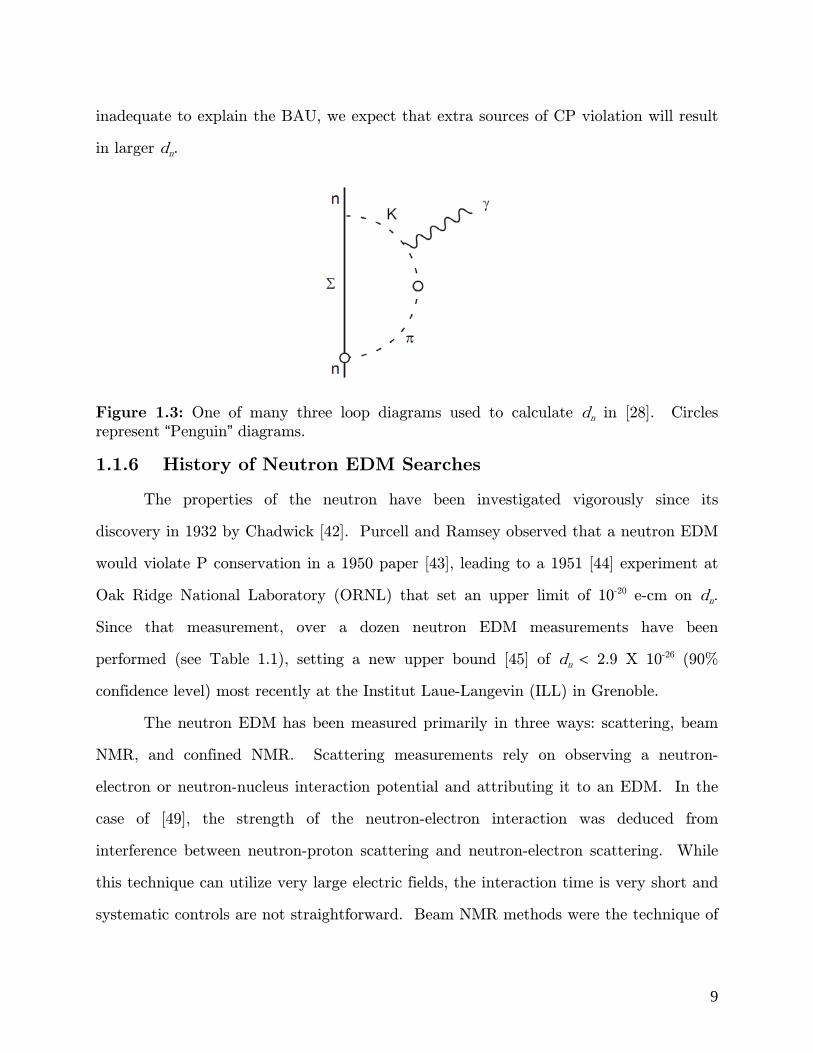
Figure 1.3: One of many three loop diagrams used to calculate dn in [28].

Circles represent “Penguin” diagrams........................................................................ 9

Figure 1.4: Observed neutron EDM upper bound versus date of experiment. The last data point is the projected measurement at SNS. Bars show the prediction ranges for dn made by the standard model [28-29], SUSY models [30-34], Multi-Higgs [37-41] and Left-Right Symmetric models [35-36]. ........................................................................................................ 12

Figure 1.5: Schematic of EDM measurement cell. 8.9 Å neutrons enter

polarized in the direction of 0B

. The cell will measure 7.6 cm X 10.2 cm X

40 cm....................................................................................................................... 13

Figure 1.6: Dispersion relation for neutrons and the elementary superfluid 4He excitation. The point of intersection is the ideal wavenumber for the incoming polarized neutrons. .................................................................................. 14

Figure 1.7: Schematic of plumbing for polarized 3He. 3He enters the accumulation volume from the polarizing atomic beam source, then travels through the plumbing into the measurement cell through the plumbing. .............. 17

Figure 1.8: Longitudinal relaxation ML of the magnetization happens when error fields transverse to B0 rotate the local magnetization vector away from B0........................................................................................................... 18

Figure 1.9: Error fields parallel (or anti-parallel) to B0 cause the magnetization to precess at different rates in different parts of the cell, leading to transverse relaxation. Spins are initially aligned at time t0 but grow out of phase at as time passes, reducing the transverse magnetization Mt of the ensemble. Dephasing of the precessing spins is shown in the reference frame rotating at the Larmor frequency. ................................................. 18

Figure 1.10: Polarized 3He atoms depolarize with probability Pd when they collide with the wall. This follows from assuming that depolarization results from passing near a highly magnetic impurity with range of interaction the mean free path of the 3He atom. ................................................. 20

Figure 2.1: Superfluid 4He film climbs from the cold part of the tube wall and evaporates in the hot area. Vapor flows down the tube and re-condenses in the cold area, delivering heat. ............................................................ 25

Figure 2.2: (a) Lower energy levels of the 3He atom. (b) Hyperfine structure of the 1083 nm transition line. ................................................................ 28

vi

Figure 2.3: Schematic for MEOP optics and RF circuit. The discharge is produced by a 15.1 MHz electric field which can be amplitude modulated to

facilitate monitoring the discharge light with a photodiode with a 1064 ± 20nm optical bandpass filter. .................................................................................. 28

Figure 2.4: Typical laser tuning signal recorded using the apparatus shown in Figure 2.3. The temperature of the laser diode controls the frequency of the laser. The lowest temperature peak is C9. The decline of the background amplitude with temperature reflects the steady degradation of the discharge during laser tuning............................................................................ 29

Figure 2.5: The polarized 3He gas handling system. Storage bottles were constructed from borosilicate glass. Plumbing was either borosilicate glass, steel, or copper tube outside of the intracell plumbing. Plumbing between the measurement cell and OPC was either borosilicate glass or 1266 stycast from Emerson and Cummings................................................................................. 31

Figure 2.6: Schematic of cryostat insert components and temperature sensor locations. Lines ending in dots point to diode temperature sensors that were monitored by a Lakeshore LS208 diode meter; lines ending in diamonds point to resistive thermal devices read out by a Lakeshore LS 370 AC resistance bridge. .............................................................................................. 33

Figure 2.7: Schematic of the plumbing for the cryostat. Major components are noted with arrows. 3He enters the 3He pot through its exhaust pipe, where it is liquefied. .......................................................................... 34

Figure 2.8: Measurement cell plumbing and thermal anchor locations. Anchor points were copper sections in the plumbing that were silver-soldered to braids that were connected to the refrigerators or top flange of the vacuum vessel, which was surrounded with liquid 4He..................................... 36

Figure 2.9: Cross section and top of the measurement cell with a rod present. Dimensions are in inches at room temperature........................................ 38

Figure 2.10: Circuit for the B0 magnet and gradient correction coil.................... 39

Figure 2.11: Shunt resistor for the B0 magnet, connected to the coil in parallel. ................................................................................................................... 40

Figure 2.12: Relative deviation of Bz from the mean in the fiducial region, in parts per million. The plot shows deviations in the field produced by the B0 magnet. The gap in the data at -400 mm is due to a large piece of the coil mount that obstructed the field mapper. Inconsistency between data sets is due in part to drifting in the magnet power supply (replaced before relaxation experiments began) during the measurements. ...................................... 42

Figure 2.13: Background field inside of cryostat, before and after steel parts in the cryostat were demagnetized with the transformer coil. The slowly varying background field that remained after degaussing was likely due to large magnetic objects in vicinity of cryostat. ............................................. 42

Figure 2.14: Degaussing coil constructed from by removing the exterior

sections of the core. The remaining section of core measured 1.5” by 1.5” and 4” long. The coil was powered by a variac...................................................... 43

Figure 2.15: Gradient coils constructed from 8 conductor cable were held on the cryostat using cable ties to tension the cables............................................. 43

vii

Figure 2.16: B1 coils are the larger pair of coils, pickup coils are the smaller set of four coils. The B1 coils were wound with the same relative direction. The two central pickup coils were wound in the opposite direction of the outer pickup coils. The measurement cell was positioned inside the central pickup coils. ................................................................................ 44

Figure 2.17: Schematic of the NMR coils and control circuit. A computer running labview controls the timing and stores data read in from the oscilloscope. Grounding one side of the pickup coils reduced the noise greatly, most likely because of a ground loop that could not be eliminated........... 46

Figure 2.18: Pulse Sequence for T2 measurement at 77 K. Optical pumping lasted for roughly 500 seconds. Current in the gradient coils could

be varied between 6p pulses in order to maximize T2.......................................... 49

Figure 2.19: Typical sequence diagram for measuring T1 using the

Injection Technique. Peaks in the “4He Storage Pres.” trace correspond to the process of filling the measurement cell with liquid 4He. The first double slash shows the break in time between the end of the liquid 4He fill and the 3He injections. The pulses in the “Optical Pumping” and “OPC 3He Pres.” traces correspond filling the OPC, polarizing the 3He gas, and injecting the

polarized gas into the measurement cell. Pulses on the “B1” and “FID

Measure” traces correspond to the T1 measurement sequence Additional injections and T1 measurements (after the second double slash mark) may follow the first, after which the cell is completely evacuated. ................................ 52

Figure 3.1: Typical background and FID signals. (a) and (b) show the background and FID signals over the entire measurement interval; (c) and (d) show the background and FID signals in the first millisecond of the measurement. .......................................................................................................... 55

Figure 3.2: FFTs of the background and FID signals shown in Figure 3.1, shown on a semi-logarithmic scale. (a) and (b) show the full FFT spectrum for the background and FID respectively; (c) and (d) show the FFT spectrum in the vicinity of the Larmor frequency for the background and FID measurements. The SNR is roughly 20 for this particular FID FFT............. 56

Figure 3.3: Total amplitude of the best fit plotted versus the phase of a 0.4 V, 16 kHz simulated FID signal. The sinusoidal dependence on the phase indicates that spectral noise plays the most important role in the uncertainty of the fit. .............................................................................................. 58

Figure 3.4: Plot of the RMS deviation in best fit amplitude versus simulated signal frequency using four different noise data sets. ............................. 59

Figure 3.5: FID Fit Amplitude vs. measurement time, shown with an exponential decay fit and 8 mV error bars. The first two points were cut from the fit on physical grounds. ............................................................................ 60

Figure 3.6: Measurement cell temperature vs. time during a typical

injection sequence, 43 2 10xD ........................................................................... 61

Figure 3.7: Results of T1 measurements with different amounts of liquid 4He in d-TPB cell, from the Ph.D. Thesis of Qiang Ye [83]. (a)T1 vs. total 4He in cell. (b) T1 vs. surface to volume ratio, using the area in contact with the bulk liquid for S. (c) T1 vs. surface to volume ratio, using the total area of the cell for S........................................................................................................ 63

viii

Figure 3.8: (a) shows the polarized 3He equilibration time vs. the initial total 3He concentration after a typical injection sequence. (b) shows the polarized 3He concentration, divided by the average concentration, vs. distance below the liquid surface at the equilibration time for the

4

3 5 10x .......................................................................................................... 65

Figure 3.9: (a) shows c2/dof for each of the T1 fits plotted vs. the measurement date. (b) shows a histogram of the residuals, with standard deviation of 9.6 mV................................................................................................. 67

Figure 3.10: (a) T1 vs. cell temperature at low concentrations. (b) T1 vs. x3. (c) T1 vs. cell temperature after the time dependence was corrected. (d) T1 vs. x3 after the time dependence was corrected. (e) T1 vs. measurement date for low concentrations. .................................................................................... 68

Figure 3.11: T1 fits for the bare Torlon rod. (a) T1 vs. measurement date for low concentrations. (b) T1 vs. cell temperature for low concentrations. (c) T1 vs. 3He concentration. (d) Cell temperature vs. measurement date. ........... 70

Figure 3.12: T1 fits for the coated Torlon Rod. T1 vs. measurement date for low concentrations. (b) T1 vs. cell temperature for low concentrations. (c) T1 vs. 3He concentration. ................................................................................... 71

Figure 3.13: (a) T1 vs. x3 for the coated BeCu rod. (b) T1 vs. Temperature for the coated BeCu rod after the concentration dependent part of the fit from Figure 3.13a was subtracted. (c) T1 vs measurement date after the concentration dependent part of the fit from Figure 3.13a was subtracted............ 72

Figure A.1: Fit to typical calibration data, taken May 1st, 2009. 8 mV

uncertainty used to compute c2/dof. ...................................................................... 80

Figure B.1: Plots of 3He concentration j vs. position at three times; the pipe runs from z=0 to 200 cm, the cells run from z=200 to 240 cm. Position is given in the unprimed coordinate. ........................................................ 84

Figure B.2: Amount of 3He in the Torlon pipe vs time and exponential fit. ....... 85

Figure B.3: Polarization loss vs. time for bare and coated Torlon. The fraction of 3He in the cells is also shown, approaching an asymptote at 86% ........ 86

ix

List of Tables Table 1.1: Summary of past neutron EDM measurements.................................. 11

Table 2.1: The volume of the polarized 3He storage bottle was determined by measuring the change in mass of the bottle after filling it completely with deionized water and measuring the mass difference with a 0.1 g accurate balance...................................................................................................... 30

Table 2.2: The calibrated volumes shown in Figure 2.4 were determined by filling the 3He storage bottle with gas, evacuating the rest of the gas handling system, then letting the gas form the 3He storage bottle expand into either a volume to be calibrated. ..................................................................... 30

Table 2.3: State of the polarized 3He gas handling system valves during different operations; O stands for open and C stands for closed, IT stands for injection technique............................................................................................. 31

Table 2.4: Details of the Helmholtz array construction........................................ 39

Table 3.1: Geometric mean of c2/dof for the empty cell data. Altering the

thermal equilibration parameter altered c2/dof only slightly. ................................ 67

Table A.1: Results of all the calibration measurements performed. The pulse column refers to the settings of the function generator used to drive the B1 coils. ............................................................................................................. 80

Table A.2: Uncertainty in T1 due to a 1% uncertainty in the calibration constant and observed statistical uncertainties from Section 3.4. .......................... 82

1

1 Introduction

A proposal was submitted by the nEDM collaboration in 2002 to undertake a

search for the EDM of the neutron using a novel technique. EDM measurements are

useful because they set limits on CP violation. There is reason to believe that there is

CP violation not currently explained within the framework of the minimal standard

model (MSM), due to the excess of matter over anti-matter in the observable universe.

Numerous theories and modifications to the MSM with extra sources of CP violation

have been proposed to explain the matter/anti-matter asymmetry, with new predictions

for the neutron EDM. A precision search for the neutron EDM will constrain or rule

out many theories beyond the MSM, which predict larger values for the neutron EDM

than predicted by the MSM.

The proposed neutron EDM search will make use of trapped ultra cold neutrons

(UCNs) precessing in a small magnetic field and large electric field. The precession rate

will be measured by observing the products of the relative spin dependent capture of

neutrons on 3He nuclei, which will precess at nearly the same rate as the neutrons. Any

modulation of the precession frequency by changing the electric field direction is

proportional to the EDM.

It is the responsibility of the University of Illinois collaborators to design and test

the systems that transport the spin-polarized 3He into the nEDM measurement cells. In

order to minimize the background from the capture of neutrons on unpolarized 3He,

materials that will be in contact with 3He in the nEDM apparatus must tested for 3He

relaxation times to assure minimal depolarization of the 3He throughout the

measurement cycle.

2

1.1 Symmetries and CP Violation

By Noether’s theorem, conserved quantities correspond to a transformation under

which the action and, if time-independent, the Hamiltonian is invariant. Three discrete

symmetry transformations, under which the Hamiltonian is usually invariant, shape our

understanding of nuclear and particle physics: Parity (P), which reverses the spatial

coordinates of a system; charge conjugation (C), the substitution of a particle with its

antiparticle; and time reversal (T), which flips the direction of the flow of time. P

violation was first observed in decays of 60Co in a magnetic field by Wu et al. [1] in

1957. CP, the combined charge conjugation and parity transformations, was thought to

be a good symmetry until the observation of CP violating neutral kaon [2] decay and

later CP violating B meson [3] decays. More recently [4], time reversal violation has

also been observed in neutral kaon decay

1.1.1 Weak Sector CP Violation in Neutral Kaon Decay

The neutral kaon strong eigenstates, 0K and 0K , are composed of ds and sd

respectively and oscillate due to the flavor changing weak interaction. A kaon can

decay weakly into two or three pion states, which have opposite values of CP. This

suggests that the neutral kaons are composed of linear combinations of the two CP

eigenstates of the Hamiltonian, referred to as K1 and K2, which undergo the following

hadronic decays:

1

0 01

02

0 0 02

K

K

K

K

There are two decay lifetimes [5] associated with neutral kaons,

8 5.17 10 sL and 11 8.93 10 s.S Due to the large difference in lifetimes, it is

easy to prepare a beam of pure KL particles, which appeared to decay only into three

pions, while the KS generally decayed into two pions. This suggested that KL was in

3

fact K2 and KS was K1. In 1964, Christenson, Cronin, Fitch, and Turlay[2] discovered

KL occasionally decays into two pions, a clear violation of CP as these two states have

opposite CP values. KL and KS are actually linear combinations of K1 and K2:

1 22

1-

1SK K K

(1.1)

2 12

1

1LK K K (1.2)

32 10 (1.3)

The CP violation due to the mixing of eigenstates is known as indirect CP

violation, which is also seen in neutral B-meson[3] decays. Direct CP violation [6] in the

neutral kaon system has also been seen in the discrepancy of the decay rate ratios in KS

and KL

0 0 0 0

L S

L S

K K

K K

p p p p

p p p p

G G

G G

(1.4)

The observed CP violation is described in the standard model as a complex phase

in the CKM matrix, but we will see this term is much too small to explain the observed

CP violation implied by the Baryon Asymmetry of the Universe (BAU) [7].

1.1.2 The BAU

The Baryon Asymmetry of the Universe (BAU), that is, the predominance of

matter over anti-matter in the observable universe, is one of the chief puzzles in

cosmology. We know that nearby (luminous) matter is composed of baryons through

direct observation – we also know, through observation of cosmic rays originating from

far away, that the asymmetry holds throughout the our galaxy since observed anti-

proton cosmic rays are consistent with interactions between cosmic rays and interstellar

matter [8]. Likewise, gamma ray backgrounds are well explained by interactions

4

between cosmic rays and normal matter [9], so that it is not necessary to resort to anti-

matter to explain them.

Figure 1.1: Plot of primordial light nuclei abundances versus baryon asymmetry parameter. Gray regions[10,11,12,13,14] show estimates of primordial abundances. Systematic errors in the estimates of abundances are not known, particularly with 7Li and D+3He. D+3He was once thought to be constant, but 3He is destroyed within stars [15] to some degree, making D+3He difficult to estimate.

Given that all observed matter generating processes produce matter and

antimatter in equal amounts, the prevalence of matter in the universe is a mystery. In

the absence of local variations in the baryon asymmetry, it seems likely that this

5

asymmetry was produced in the early universe, by processes as yet unobserved in the

laboratory.

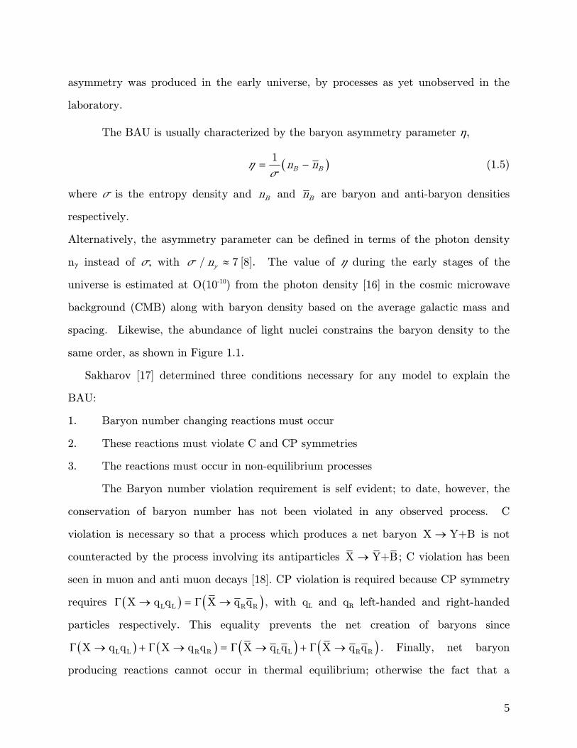
The BAU is usually characterized by the baryon asymmetry parameter ,

1B Bn nh

s (1.5)

where s is the entropy density and Bn and Bn are baryon and anti-baryon densities

respectively.

Alternatively, the asymmetry parameter can be defined in terms of the photon density

ng instead of s, with / 7ngs [8]. The value of h during the early stages of the

universe is estimated at O(10-10) from the photon density [16] in the cosmic microwave

background (CMB) along with baryon density based on the average galactic mass and

spacing. Likewise, the abundance of light nuclei constrains the baryon density to the

same order, as shown in Figure 1.1.

Sakharov [17] determined three conditions necessary for any model to explain the

BAU:

1. Baryon number changing reactions must occur

2. These reactions must violate C and CP symmetries

3. The reactions must occur in non-equilibrium processes

The Baryon number violation requirement is self evident; to date, however, the

conservation of baryon number has not been violated in any observed process. C

violation is necessary so that a process which produces a net baryon X Y+B is not

counteracted by the process involving its antiparticles X Y+B ; C violation has been

seen in muon and anti muon decays [18]. CP violation is required because CP symmetry

requires L L R RX q q X q qG G , with qL and qR left-handed and right-handed

particles respectively. This equality prevents the net creation of baryons since

L L R R L L R RX q q X q q X q q X q qG G G G . Finally, net baryon

producing reactions cannot occur in thermal equilibrium; otherwise the fact that a

6

baryon and corresponding anti-baryon have the same energy will force these two species

back into equal densities. This condition can be satisfied, for example, during bubble

nucleation in the electroweak phase transition.

1.1.3 Strong CP violation in the MSM

In addition to the CP violating phase in the CKM matrix, there is potential CP

violation in the MSM from an explicit CP violating term in the generalized QCD

Lagrangian [19], the so-called “q term”, which is permissible because it does not alter the

QCD action.

,2

232

mnmnqq p

a agL G G (1.6)

,1

2

a aG G (1.7)

G is the gluonic field strength tensor (analogous to F mn in electromagnetism) and G is

its dual. GG violates CP since it is proportional to E B

, which violates P but

conserves C. From the 199Hg EDM measurement by Romalis et al. in 2000 [20],

101.5 10q . The very small size of this term, which has a natural scale of 2p, is

known as the strong CP problem. One proposed solution to this problem is the Peccei-

Quinn [21] theory, which posits that q is a field rather than a constant, resulting in a

new symmetry that, when broken, produces a Goldstone boson (as yet undetected)

known as the axion. After this symmetry breaking, q is reduced to 0.

1.1.4 Modifications to the Minimal Standard Model (MSM)

The CP violating mechanisms in the MSM appear to be insufficient [22] to

explain the BAU; however, many modifications to the MSM with extra sources of CP

violation have been proposed. One of the simpler ideas is the presence of heavy right-

handed Majorana neutrinos in the early universe: Such a neutrino is its own CPT

image and would violate lepton number when it decayed because of interference between

7

the tree level diagram and the one-loop radiative correction [23]. This lepton-antilepton

asymmetry could be transmitted to baryons through processes mediated by sphalerons,

which are non-perturbative gauge fields that conserve B L rather than B L .

Shaposhnikov [24] proposed such a model (called nMSM) with three heavy, sterile, right-

handed neutrinos. The model explains the light mass of the active neutrinos through

the see-saw mechanism,

22

, ,i I i

i

m mf

v

n (1.8)

with Yukawa couplings fi , active neutrino masses mn,i , sterile neutrino masses mI,i, and

Higgs vacuum expectation value v. The lightest sterile neutrino is stable, accounting for

the dark matter in the universe.

CP violation is also possible in supersymmetric theories, which add a bosonic

(fermionic) superparter for each elementary fermion (boson). If they exist, the masses of

the superpartners must be quite high since they have not yet been detected. Many new

CP violating phases are produced (in the supersymmetry analog of the CKM matrix) by

supersymmetry breaking [25]. Among other reasons, supersymmetry is an attractive

theory because it can explain dark matter through a stable lightest superpartner [26],

solves the problem of renormalization of the weak interaction above 1 TeV and produces

gauge coupling unification [27].

1.1.5 Using the Neutron EDM to Measure CP Violation

Particle EDMs violate time reversal and parity symmetries, and therefore CP

symmetry, by the CPT theorem. This makes EDMs a useful model-independent tool for

measuring CP violation. Both violations arise from the fact that a particle EDM vector

must be aligned with the spin vector, because there are no additional degrees of freedom

available for the EDM. Under parity reversal, an EDM flips while the spin magnetic

8

moment is unchanged; under time reversal, the spin magnetic moment flips while the

EDM is unchanged. These transformations are shown in Figure 1.2.

Consider an experiment where the precession of a spin magnetic moment in a

magnetic field is measured. The EDM precesses in the magnetic field along with the

spin; adding an electric field alters the precession rate by an amount proportional to the

magnitude of the EDM. The neutron is a natural candidate for this type of experiment

if a sufficient number of neutrons can be produced and confined.

Figure 1.2: a) The parity transformation reverses the EDM direction but leaves the spin unchanged. b) Time reversal changes the direction of the spin but leaves the EDM unchanged.

MSM predictions for the neutron EDM, dn, arising from the CKM phase

contribution are very small, ranging from 10-30 e-cm [28] to 10-32 e-cm [29], because they

arise, to lowest order, from three-loop Feynman diagrams. Such small values for dn will

not be experimentally accessible in the foreseeable future. However, there are reasons to

expect that dn may be substantially larger than the MSM predicts. Numerous theories

beyond the MSM, which are already constrained by past EDM searches, predict a larger

value for dn: Supersymmetric (SUSY) extensions of the SM [30,31,32,33,34], left-right

symmetric models [35,36] and a class of non-minimal models in the Higgs

[37,38,39,40,41] sector have CP violation mechanisms not present in the MSM with dn

prediction ranges in Figure 1.4. Furthermore, since the CKM phase appears to be

9

inadequate to explain the BAU, we expect that extra sources of CP violation will result

in larger dn.

Figure 1.3: One of many three loop diagrams used to calculate dn in [28]. Circles

represent “Penguin” diagrams.

1.1.6 History of Neutron EDM Searches

The properties of the neutron have been investigated vigorously since its

discovery in 1932 by Chadwick [42]. Purcell and Ramsey observed that a neutron EDM

would violate P conservation in a 1950 paper [43], leading to a 1951 [44] experiment at

Oak Ridge National Laboratory (ORNL) that set an upper limit of 10-20 e-cm on dn.

Since that measurement, over a dozen neutron EDM measurements have been

performed (see Table 1.1), setting a new upper bound [45] of dn < 2.9 X 10-26 (90%

confidence level) most recently at the Institut Laue-Langevin (ILL) in Grenoble.

The neutron EDM has been measured primarily in three ways: scattering, beam

NMR, and confined NMR. Scattering measurements rely on observing a neutron-

electron or neutron-nucleus interaction potential and attributing it to an EDM. In the

case of [49], the strength of the neutron-electron interaction was deduced from

interference between neutron-proton scattering and neutron-electron scattering. While

this technique can utilize very large electric fields, the interaction time is very short and

systematic controls are not straightforward. Beam NMR methods were the technique of

10

choice in the 1960’s and 1970’s. In this technique, polarized neutrons in a beam precess

in the presence of applied magnetic and electric fields. Precession is measured by the

separated oscillatory field method [46] developed by Norman Ramsey. The beam NMR

method allowed much longer interaction times, of order milliseconds, and control of the

applied electric field. Beam methods were ultimately limited by the systematic error

from the motional magnetic field,

v E , which contributed to a false EDM when

B

and

E were misaligned. The advent of ultra cold neutrons (UCNs, mean speed <7.6

m/s) allowed much longer interaction times since UCNs could be stored in a container

(because very slow neutrons are reflected from the ~200 eV Fermi Potential [47,48]) for

a substantial fraction of the neutron lifetime. The

v E systematic was also eliminated

to first order since the average velocity of the confined neutrons was zero. The chief

shortcoming of the confined UCN approach is that high densities of UCNs are difficult

to achieve. UCNs are typically produced from a thermal neutron source with a mean

velocity that is much too high – UCNs are accumulated from the low-speed tail of the

Maxwell velocity distribution.

The nEDM collaboration has proposed a new measurement of the neutron EDM

at the Spallation Neutron Source (SNS) in Oak Ridge, TN which has the potential to

reduce the upper bound of the neutron EDM by about two orders of magnitude. The

keys to this improvement in precision are a 4X longer measurement time, 5X higher

electric field strength and 50X higher UCN density than used in the most recent

measurement at the ILL. These improvements rely on a unique method of UCN

production in liquid 4He that overcomes the limitations of the thermal neutron source

while increasing the dielectric strength inside the measurement cell.

11

Ex. Type v E B Coh. UC EDM Ref.

(Lab) (m/sec (kV/cm (Gauss (sec) (cm- (e - cm ) (year)

Scattering 2200 ~ 1015 — ~ 10-20 — [49]

(ANL) < 3 X10-18 (1950)

Beam Mag. 2050 71.6 150 0.00077 — (–0.1 ≤ 2.4) X10-20 [50]

(ORNL) < 4 X10-20 (90% C.L.) (1957)

Beam Mag. 60 140 9 0.014 — (–2 ≤ 3) X 10-22 [51]

(ORNL) < 7 X 10-22 (90% C.L.) (1967)

Bragg 2200 ~ 109 — ~ 10-7 — (2.4 ≤ 3.9) X 10-22 [52]

(MIT/BNL) < 8 X 10-22 (90% C.L.) (1967)

Beam Mag. 130 140 9 0.00625 — (–0.3 ≤ 0.8) X 10-22 [53]

(ORNL) < 3 X 10-22 (1968)

Beam Mag. 2200 50 1.5 0.0009 — [54]

(BNL) < 1 X 10-22 (1969)

Beam Mag. 115 120 17 0.015 — (1.54 ≤ 1.12) X 10-23 [55]

(ORNL) < 5 X 10-23 (1969)

Beam Mag. 154 120 14 0.012 — (3.2 ≤ 7.5) X 10-24 [56]

(ORNL) < 1 X 10-23 (80% C.L.) (1973)

Beam Mag. 154 100 17 0.0125 — (0.4 ≤ 1.5) X 10-24 [57]

(ILL) < 3 X 10-24 (90% C.L.) (1977)

UCN Mag. <7.6 25 0.028 5 — (0.4 ≤ 0.75) X 10-24 [58]

(PNPI) < 1.6 X 10-24 (90% C.L.) (1980)

UCN Mag. <7.6 20 0.025 5 2.5 (2.1 ≤ 2.4) X 10-25 [59]

(PNPI) < 6 X 10-25 (90% C.L.) (1981)

UCN Mag. <7.6 10 0.01 60–80 0.05 (0.3 ≤ 4.8) X 10-25 [60]

(ILL) < 8 X 10-25 (90% C.L.) (1984)

UCN Mag. <7.6 12–15 0.025 50–55 — – (1.4 ≤ 0.6) X 10-25 [61]

(PNPI) < 2.6 X 10-25 (95% C.L.) (1986)

UCN Mag. <7.6 16 0.01 70 10 – (3 ≤ 5) X 10-26 [62]

(ILL) < 12 X 10-26 (95% C.L.) (1990)

UCN Mag. <7.6 12–15 0.018 70-100 — (2.6 ≤ 4.5) X 10-26 [63]

(PNPI) < 9.7 X 10-26 (90% C.L.) (1992)

UCN Mag. <7.6 4.5 0.01 120-150 1 (–1 ≤ 3.6) X 10-26 [64]

(ILL) < 6.3 X 10-26 (90% C.L.) (1999)

UCN Mag. <7.6 1100 00..0011 112200 1 [45] (ILL) < 2.9 X 10-26 (90% C.L.) (2006)

UCN Mag. <7.6 50 0.01 500 75

(SNS) ~10-28 (~2016)

Table 1.1: Summary of past neutron EDM measurements.

12

Figure 1.4: Observed neutron EDM upper bound versus date of experiment. The last data point is the projected measurement at SNS. Bars show the prediction ranges for dn

made by the standard model [28-29], SUSY models [30-34], Multi-Higgs [37-41] and Left-Right Symmetric models [35-36].

1.2 The Proposed Measurement at SNS

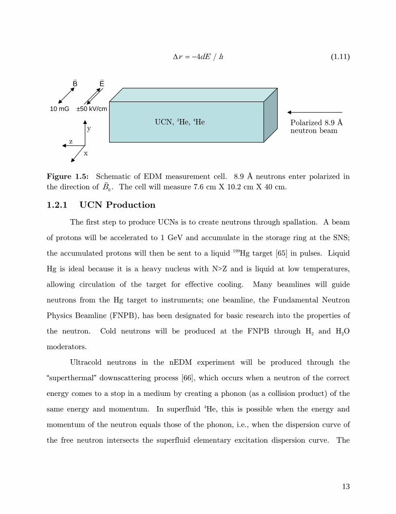
The neutron EDM measurement at SNS will be performed in a two cell system,

shown in Figure 1.5: Each cell will be filled with liquid 4He at 400 mK. One cell will

have an electric field of 50 kV/cm, the other will have an electric field of -50 kV/cm.

Both cells will have magnetic field 0 0 0 10, mGB B x B

. The electric fields will be

reversed occasionally so that any systematic differences between the cells will be

controlled.

The EDM measurement will be performed as follows: Neutrons will enter the

cells polarized in the direction of B0. A pulse will rotate the neutrons and precession

will occur until the neutrons have decayed away. The precession rate in the cell with a

positive (negative) electric field will be pos (neg):

02 /pos B dE hn m (1.9)

02 /neg B dE hn m (1.10)

13

4 /dE hn (1.11)

Figure 1.5: Schematic of EDM measurement cell. 8.9 Å neutrons enter polarized in

the direction of 0B

. The cell will measure 7.6 cm X 10.2 cm X 40 cm.

1.2.1 UCN Production

The first step to produce UCNs is to create neutrons through spallation. A beam

of protons will be accelerated to 1 GeV and accumulate in the storage ring at the SNS;

the accumulated protons will then be sent to a liquid 199Hg target [65] in pulses. Liquid

Hg is ideal because it is a heavy nucleus with N>Z and is liquid at low temperatures,

allowing circulation of the target for effective cooling. Many beamlines will guide

neutrons from the Hg target to instruments; one beamline, the Fundamental Neutron

Physics Beamline (FNPB), has been designated for basic research into the properties of

the neutron. Cold neutrons will be produced at the FNPB through H2 and H2O

moderators.

Ultracold neutrons in the nEDM experiment will be produced through the

“superthermal” downscattering process [66], which occurs when a neutron of the correct

energy comes to a stop in a medium by creating a phonon (as a collision product) of the

same energy and momentum. In superfluid 4He, this is possible when the energy and

momentum of the neutron equals those of the phonon, i.e., when the dispersion curve of

the free neutron intersects the superfluid elementary excitation dispersion curve. The

B

E

UCN, 3He, 4He

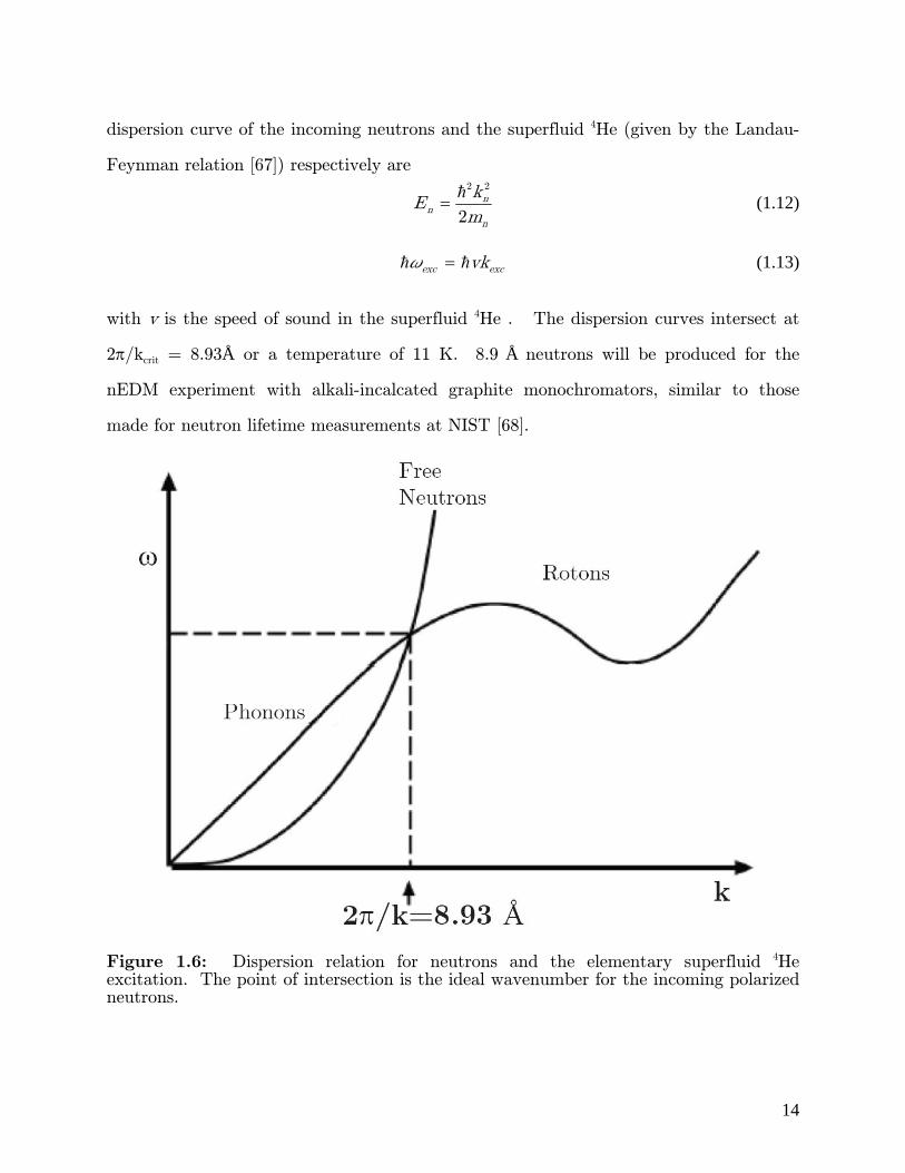
x

z

y Polarized 8.9 Å neutron beam

10 mG ±50 kV/cm

14

dispersion curve of the incoming neutrons and the superfluid 4He (given by the Landau-

Feynman relation [67]) respectively are

2 2

2n

n

n

kE

m (1.12)

exc excvkw (1.13)

with v is the speed of sound in the superfluid 4He . The dispersion curves intersect at

2/kcrit = 8.93Å or a temperature of 11 K. 8.9 Å neutrons will be produced for the

nEDM experiment with alkali-incalcated graphite monochromators, similar to those

made for neutron lifetime measurements at NIST [68].

Figure 1.6: Dispersion relation for neutrons and the elementary superfluid 4He excitation. The point of intersection is the ideal wavenumber for the incoming polarized neutrons.

15

The UCNs may be upscattered by absorbing a phonon, but the upscattering

cross-section sup is smaller than the downscattering cross section sdown by a factor of E

kTe

, since by the principle of detailed balance,

UCN up UCN downB

Ek TE E E es s

(1.14)

where E is the energy of the phonon and T ~ 0.45 K is the temperature of the 4He bath.

In addition, very few such phonons are available since their density in the superfluid

varies with T4 [67].

Superfluid 4He has two other beneficial qualities for a neutron EDM experiment.

It does not absorb neutrons and it can tolerate large electric fields. The first property

means that neutron storage times approaching the neutron lifetime are possible with the

proper wall material (and 3He concentration in the superfluid 4He, which will be

discussed later). The second property will allow the neutron EDM experiment at SNS

to be performed at a planned electric field of 50 kV/cm, five times larger than the

electric field used in the recent ILL experiment.

1.2.2 Neutron Precession Measurement

The precession of the neutron spins will be observed by means of polarized 3He,

which will reside in the same superfluid 4He volume that holds the neutrons. The 3He

will enter the cryostat from a cold atomic beam source, which will polarize the 3He

nuclei using a quadrupole magnet. Since the gyromagnetic ratios of 3He and neutrons

are only 11% different [69], the 3He and UCNs will be tipped by 90 degrees using a

single pulse; this is possible despite the difference in precession rates by applying a pulse

that is off resonance for both species. The spin of the neutrons will be detected by the

relative-spin dependent capture reaction, 3 764 keVHe n p t , with capture cross

section at 5 m/s roughly 106 [70] barns when the spins are anti-parallel and ~0 with

spins parallel The reaction products will produce excited states as they pass through

the liquid 4He, which in turn will produce ultraviolet light. The ultraviolet light will

16

cause the d-TPB cell wall coating [71] to scintillate, producing light that will be

detected by photomultiplier tubes. Since the capture cross section is highly dependent

on the relative orientation of the neutron and 3He spins, the light signal oscillates at the

rate of the relative precession of 3He and the neutrons. The 3He concentration, x3, of

roughly one 3He atom per 1010 4He atoms is determined by the competing requirements

of maximal signal and maximal measurement time; too many 3He atoms will result in a

high neutron capture rate that reduces the useful measurement time substantially. The

usefulness of this technique to measure a neutron EDM is contingent on 3He having

zero, or a very small EDM. Since the 3He nucleus is surrounded by a complete 1s

electron shell, any nuclear EDM of 3He is suppressed by Schiff [72] shielding.

The 3He will also be used to measure the magnetic field in the two measurement

cells by observing 3He precession with SQUID magnetometers, acting as a co-

magnetometer. This will allow any changes in the magnetic environment of the cell to

be tracked. Over time the 3He will become unpolarized due to relaxation mechanisms

which are discussed below; because of this, it is necessary to remove the 3He at the end

of each measurement cycle and replenish it with fresh polarized 3He. Unpolarized 3He is

a significant potential problem because it will produce a background, since it will

capture neutrons at a steady rate. There are several ways that unpolarized 3He can

accumulate in the measurement cells. The atomic beam source itself will start with a

polarization slightly under 100%. Polarization losses will also occur in the 3He

accumulation volume (Figure 1.7) and the plumbing between between the accumulation

volume and the measurement cell. Finally, the 3He will be depolarized in the

measurement cell itself, which will be valved off from the plumbing during the

measurement cycle.

17

Figure 1.7: Schematic of plumbing for polarized 3He. 3He enters the accumulation volume from the polarizing atomic beam source, then travels through the plumbing into the measurement cell through the plumbing.

1.3 3He Relaxation

Within the superfluid 4He, there are two basic kinds of polarization loss (or

relaxation) that affect the ensemble of spins. Longitudinal relaxation results from

perturbations in the magnetic field that locally rotate magnetization non-adiabatically

away from 0B

, resulting in exponential decay of the longitudinal magnetization with

time constant T1. These perturbations are of the form or i ix z x yB B , since gradients

in xB do not cause spins to rotate away from the holding field (which points along x ).

Figure 1.8 shows how perturbations in the magnetic field cause T1 decay. Transverse

relaxation takes place during precession and results from variations in the magnitude of

B0, i.e., gradients of the form Bix x . These local variations in Bx result in different

regions of the cell precessing at different rates, as shown in Figure 1.9. As these regions

get out of phase, the measurable signal due to precession decays with lifetime T2. 3He

spin relaxation in the EDM cells can arise from two sources: long range gradients due to

magnet design or shielding flaws, and short range gradients at the walls of the cells.

Accumulation volume

Plumbing

Measurement Cell

Polarized 3He from ABS

Valves

18

Figure 1.8: Longitudinal relaxation ML of the magnetization happens when error fields transverse to B0 rotate the local magnetization vector away from B0.

Figure 1.9: Error fields parallel (or anti-parallel) to B0 cause the magnetization to precess at different rates in different parts of the cell, leading to transverse relaxation. Spins are initially aligned at time t0 but grow out of phase at as time passes, reducing the transverse magnetization Mt of the ensemble. Dephasing of the precessing spins is shown in the reference frame rotating at the Larmor frequency.

1.3.1 Long Range Magnetic Gradients The effect of constant long range gradients depend on the motion of the 3He

atoms within the cells: rapid transit through the cell tends to increase T2 since

dB

B0 ML0

ML1

M0

M1

B0 dB

t = t0 t = t1

Mt,0 Mt,1

19

dephasing is partially averaged out when the atom samples the whole cell. On the other

hand, T1 is decreased by rapid transit of 3He atoms, as this increases the rate the atom

sees field fluctuations. T2 for polarized gas in a gradient was predicted analytically by

McGregor [73]. For a cylindrical cell of radius a and length L containing a spin-

polarized fluid with diffusion constant D, the relaxation times are given by:

222 4 2 4

2 1

1 1 7

2 120 96

x xL B a B

T T D z D y

(1.15)

This gives a good first order estimate for the EDM cell, which is rectangular but much

longer than it is wide. The last term in Equation 1.14 can safely be ignored since

L4>>a4. T1 for a polarized gas was worked out by Schearer and Walters [74] for a gas in

constant gradient G, of the form or i ix z x yB B for B0 along x, and mean collision time

tc and is given by:

12

2

0

21

312 1

B DGD

T B v

g

(1.16)

2

3

cv tD (1.17)

The target values for T1 and T2 are both 10,000 s, which leads to roughly 90%

polarization after the expected measurement time of 1000 s.

The diffusion constant in the neutron EDM experiment will depend only on the

interaction between 3He and phonons in the superfluid 4He, since 3He-3He interactions

will be insignificant at x3 = 10-10. As a result, the 3He in solution will have a diffusion

constant of D34 = 1.6T-7 cm2/s [75]. At any temperature considered for the nEDM

experiment, the second term in parentheses in (1.18) can be ignored because the 2v

term in the denominator will be very large compared to 3g B0D. The very rapid

temperature dependence of D34 has substantial implications on the design and operating

20

temperature of experiment, as can be seen in the following calculations. For B0 = 10

mG and the gradient design goal G < 0.05 mG/cm, this leads to T1 ~ 4 X 107 s and T2 ~

20,000 s at 0.45 K and T1 ~ 3 X 106 s and T2 ~ 300,000 at 0.3 K. These times are more

than acceptable for EDM (though T2 at higher temperatures may be of concern), but

wall effects must also be evaluated.

1.3.2 Wall Relaxation

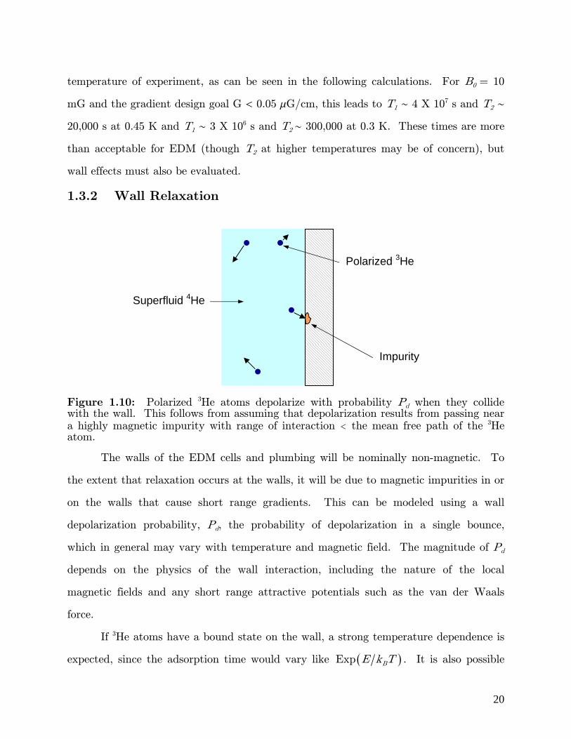
Figure 1.10: Polarized 3He atoms depolarize with probability Pd when they collide with the wall. This follows from assuming that depolarization results from passing near a highly magnetic impurity with range of interaction the mean free path of the 3He atom.

The walls of the EDM cells and plumbing will be nominally non-magnetic. To

the extent that relaxation occurs at the walls, it will be due to magnetic impurities in or

on the walls that cause short range gradients. This can be modeled using a wall

depolarization probability, Pd, the probability of depolarization in a single bounce,

which in general may vary with temperature and magnetic field. The magnitude of Pd

depends on the physics of the wall interaction, including the nature of the local

magnetic fields and any short range attractive potentials such as the van der Waals

force.

If 3He atoms have a bound state on the wall, a strong temperature dependence is

expected, since the adsorption time would vary like Exp BE k T . It is also possible

Impurity

Polarized 3He

Superfluid 4He

21

that 3He spends some time diffusing in pores on the wall or the solid 4He film coating

the wall. Pd will depend on B0 if impurities are ferromagnetic in nature since in general

1 2

1 0T B BD and the perturbing field DB will be determined by the permanent

magnetization of the impurity. On the other hand, a paramagnetic impurity (such as

O2 contamination) will lead to constant Pd since the perturbing field will be proportional

to B0. In experiments [76] with polarized 3He gas on a superfluid 4He film coated pyrex

cell, Lusher et al. observed a 2 to 3 order of magnitude increase in T1 after the pyrex

cell was baked at 470 °C under a vacuum of 1 mTorr, presumably due to the removal of

O2 molecules from the wall.

The longitudinal wall relaxation rate is given by Pd multiplied by the polarized

atom collision rate, divided by the total number of polarized atoms. The polarized atom

collision rate is [77]

,

1

4p

c p

Nv S

Vn (1.18)

v is the mean speed of the 3He quasiparticles (the collective excitation from Landau-

Fermi theory with mass *

3 2.3m m [67]), Np is the total number of polarized atoms,

V is the volume of the liquid, and S is the surface area of the wall. The factor of ¼

comes from the Maxwell velocity distribution along with the fact that half of the atoms

are moving toward the wall and half away from it. Therefore the relaxation rate, g, is

given by

, 1

4

c p

d

p

SP v

N V

ng (1.19)

with the mean speed *8 /Bv k T mp from the Maxwell distribution. S/V for the

EDM cell is 1579 cm2 / 3100 cm3 =0.51 cm-1. In the EDM cell at 0.45 K, Pd must be

less than 72 10 to achieve T1 > 10,000 s.

22

1.3.3 Wall Materials

There are several regions in the EDM apparatus that will require minimal 3He

wall depolarization. As mentioned in Section 1.3.3, the measurement cell will be coated

with a wavelength shifter that converts UV (emitted from excitations in the liquid 4He)

into visible light. The coating must have a good neutron lifetime and T1 > 10,000 s.

TPB is ideal if the hydrogen atoms (which can absorb UCNs) are replaced with

deuterons. TPB dissolves in toluene, which allows easy application to acrylic, and

makes a good optical coating on acrylic when the TPB is mixed with polystyrene in the

toluene. Deuterated versions of TPB, polystyrene, and toluene are all commercially

available, though rare in the case of TPB, and are all hydrocarbons, which should make

the wall coating non-magnetic.

The plumbing that will bring polarized 3He into the experimental cells does not o

have a neutron lifetime requirement, but it must minimally depolarize the 3He in order

to reduce the background from unpolarized 3He in the EDM measurement cells. A

material that thermally contracts like a metal, but containing very little magnetic

material, will make it easier to couple the plumbing using metal flanges. This is useful

because it will not be possible to make all the plumbing out of one piece, and gluing

multiple pieces in situ will make disassembly impossible. Metal plumbing, however, will

likely be problematic due to magnetic impurities present in most commercially available

alloys, and also because of the trapped flux from any low temperature superconductors.

Torlon (polyamide-imide) is a nominally non-magnetic, opaque, plastic that thermally

contracts at nearly the same rate as copper; the current design utilized Torlon for most

of the plumbing. Other plastics may be used in the system, but will present difficulties

due to differential thermal contraction.

Polarized 3He will briefly pass through valves, so these valves must be

constructed from materials that do not immediately depolarize the 3He. Relaxation

times of 10,000 s are not necessary, but ideally T1 should be longer than 100 s in the

23

valve. The valve seat and stem will be constructed from a hard plastic such as Vespel

or Torlon and are not likely to be problematic. The valve body will likewise be

constructed from plastic. The motion of the valve requires a bellows type seal, which

must be made from metal. Stainless steel is normally used for this purpose, but almost

certainly will depolarize the 3He very quickly. Beryllium copper bellows should be less

magnetic and can be obtained commercially. Unfortunately, this alloy contains a small

amount of nickel, which is ferromagnetic and potentially problematic. The wall

relaxation time in the bellows may be improved by coating it with polyamide-imide

(PAI) resin, which should survive thermal cycling well because of the aforementioned

good thermal contraction mating to copper.

In order of importance, deuterated TPB, PAI coated BeCu, and Torlon must be

tested. Deuterated TPB is most important because there is no way to mitigate a short

3He lifetime in the cell. The PAI resin coated BeCu is the next most important because

there is a reasonable chance that, even coated, the bellows will depolarize the 3He. If

this is the case, a workaround must be found while nEDM is still in the design stages.

It would be very nice if off-the-shelf Torlon works out as the plumbing material, but it

is not the only conceivable material – it is possible, for example, to coat the t

1.3.4 Small Scale Materials Test

Before the design for the nEDM experiment can be finalized, these materials

must be tested to ensure a sufficiently small 3He depolarization probability, Pd. In

general, test cells must be constructed on a much smaller scale than the nEDM

experiment due to the expense of a cryostat that could accommodate the full size

apparatus. nEDM collaborators are responsible for the overall 3He system including the

plumbing and ensuring that materials used in nEDM will not excessively depolarize the

3He. There are three key differences between a small scale cell and the EDM cell: S/V,

the cell surface to volume ratio, will be larger in the small scale cell, leading to a smaller

24

value for T1; the concentration of 3He in superfluid 4He will be much higher, between 10-

4 and 10-3, in the small scale experiment, since a SQUID magnetometer would be

necessary for measurements at the EDM concentration of 10-10. Finally, the magnetic in

the Illinois small scale experiment will be much larger (5 G instead of 10 mG) to enable

inductive detection of the 3He precession. These differences are not expected to

significantly affect the determination of Pd.

25

2 Method

The technique for measuring the relaxation time of 3He in superfluid 4He is

discussed below: a brief description of requirements for the apparatus is described,

followed by detailed descriptions of the major components, and finally the measurement

techniques.

2.1 Design Requirements

In order to measure Pd, it was necessary to produce enough polarized 3He to

produce a NMR signal with adequate S:N. It was necessary to transport the polarized

3He into the measurement cell, which was filled with superfluid 4He, and cool it to 0.45

K. This was challenging because of the heat load due to flowing superfluid 4He, which

flowed into warm areas, evaporated, and re-condensed in cold areas (Figure 2.1).

Figure 2.1: Superfluid 4He film climbs from the cold part of the tube wall and evaporates in the hot area. Vapor flows down the tube and re-condenses in the cold area, delivering heat. Polarized 3He was produced using metastability exchange optical pumping

(MEOP) [78] due to its simpler implementation compared to other techniques [79,80];

Q

Q

Hot

Cold

26

MEOP allowed the use of a small (few Gauss) B0 field and a substantial polarized 3He

production rate. The main limitations of MEOP are that it can only be performed in

3He with pressure < 10 Torr (13 mBar) [81], and it is very sensitive to contamination.

The following simple calculation demonstrates the viability of MEOP, using

numbers that were typical during T1 measurements: assuming a spin excess fraction

(henceforth polarization) 10%p is produced in an Optical Pumping Cell (OPC) at

room temperature, with volume 200 mLOPCV and filled to 1 TorrOPCp , is injected

into a measurement cell with volume 20 mLMCV (all 3He ends up in the

measurement cell), then the maximum possible magnetization produced in the

measurement cell using MEOP is 3

maxM pnm , with 3He nuclear magnetic moment m3,

polarization fraction 10%p , and density in the measurement cell

OPC OPC A

ATM molar MC

p V Nn

p V V (2.1)

max 3OPC OPC A

ATM molar MC

p V NM p

p V Vm (2.2)

Vmolar is the volume of 1 mole of gas at 300 K and 1 bar, and 1 barATMp . Using

dimensional analysis, we expect the induced voltage in a 1” by 4” rectangular pick up

coil to be roughly

0 maxind coil LarmorV M Am w

(2.3)

with 16.2 kHzLarmorw in a 5 G magnetic field. This leads to an induced voltage of 0.1

mV per turn in this calculation, which overestimates the flux since the magnetic field

inside the coils will be less than 0

maxMm . Coils with a few hundred turns are easy to

wind, leading to a signal in the tens of microvolts, which is measurable if the pickup

27

coils are well shielded. MEOP in a two cell system with 10OPC MCV V therefore

produces an adequate signal for T1 measurements.

Cooling a cell filled with superfluid 4He requires careful design and significant

cooling power in the 0.3 K range. The heat load into the cell due to superfluid 4He film

flow should be of order 100 mW if the cell hangs from a 1 mm I.D. capillary [82]. A 3He

evaporative refrigerator [83] is capable of providing 100 mW cooling power at 0.35 K,

which is adequate if thermal connections are made properly. A 3He evaporative

refrigerator is preferable to a dilution refrigerator since it is simpler, which allowed it to

be custom built in Illinois using non-magnetic parts wherever possible.

2.2 Polarized 3He Production

2.2.1 Optical Pumping

As mentioned above, polarized 3He is produced by MEOP at room temperature.

MEOP utilizes a weak RF discharge in a glass cell to populate the 3He 23s1 metastable

excited state, along with many other excited states. The 23s1 electron can be excited

further into a spin ½ 23p0 state (Figure 2.2 [78].) by means of a circularly polarized 1083

nm laser. This spin then can be transferred to the 3He nucleus by the hyperfine

interaction. This process yields a polarization of order 10% [81] with a low power laser

at pressures near 1 Torr.

A tunable, 80 mW, 1083 nm (100 MHz bandwidth) Distributed Bragg Reflector

(DBR) diode laser was purchased from Eagleyard and mounted on a Thorlabs TCLDM3

TO-3 type laser mount, controlled by Thorlabs ITC 502 laser controller. The light from

the laser, which was intrinsically linearly polarized, passed through a convergent lens

and 1064 ±10 nm Quarter Wave Plate (QWP) in order to produce nearly circularly

polarized light; a 1064 nm QWP was used since a 1083 nm QWP was not readily

available. The optics for the laser and the circuit to produce the rf discharge are shown

schematically in Figure 2.3

28

Figure 2.2: (a) Lower energy levels of the 3He atom. (b) Hyperfine structure of the 1083 nm transition line.

Figure 2.3: Schematic for MEOP optics and RF circuit. The discharge is produced by a 15.1 MHz electric field which can be amplitude modulated to facilitate monitoring the

discharge light with a photodiode with a 1064 ± 20nm optical bandpass filter.

The C9 (Figure 2.2) transition produces the highest polarization when optically

pumping 1 Torr of 3He [81]; the laser was tuned to the C9 peak by measuring 1083 nm

light intensity with a Thorlabs PDA520 photodiode with a 1064 ±20 nm optical band

pass filter, monitored by a SRS 830 lock-in detector as the laser temperature (and

therefore wavelength) was adjusted. Peaks in 1083 nm light correspond to the de-

Diode Mount

Convergent Lens Diode QWP Mirror

RF Amp RF Out

RF In

Mod In

Photo-diode

Lock-In Amp Mod Out

Signal In

RF Signal Generator

RF Out

5:1 Transformer

Laser Controller

Amp Out

Data Logger

MEOP Cell

Electrodes Trim Cap

(a) (b)

29

excitation of levels populated by the laser. Figure 2.4 shows a typical laser fluorescence

peak measurement in a moderately clean cell.

The discharge was created by high voltage RF electrodes, shown in Figure 2.3,

made from copper tape placed on the outside of the cell. High voltage RF was produced

with a HP 8647A signal generator amplified by an ENI 525 LA amplifier. This voltage

was stepped up by a hand wound air core 5:1 transformer in a tank circuit with a

tunable RF capacitor to produce high voltage at the cell while minimizing noise

transmitted by the long RF cable leading to the step-up circuit.

Figure 2.4: Typical laser tuning signal recorded using the apparatus shown in Figure 2.3. The temperature of the laser diode controls the frequency of the laser. The lowest temperature peak is C9. The decline of the background amplitude with temperature reflects the steady degradation of the discharge during laser tuning.

2.2.2 3He Gas System for the OPC

The gas handling system for the polarized 3He is shown in Figure 2.5. The

storage bottles were filled with 3He or 4He and the amount of gas present was measured

with a 1000 Torr MKS 626A13TBE baratron pressure transducer. Plumbing was

constructed mostly from borosilicate glass to reduce outgassing which might

contaminate the 3He in the OPC. The 3He storage bottle volume was calibrated by

observing the increase in mass by filling it with de-ionized water (Table 2.1). Other

volumes were calibrated in turn by filling the calibrated 3He storage bottle with helium

30

gas and expanding it into other volumes while measuring the reduction in pressure

(Table 2.2). The OPC was filled from the storage bottles through a SAES PS2GC50R1

getter, which absorbed all non-noble atmospheric gases. However, a substantial

amount of plastic was used in the low temperature plumbing above measurement cell

(after the getter) in order to reduce depolarization of the 3He, since the adsorption

energy of pyrex is much larger than plastic. As a result, plastic vapor entered the OPC

if MEOP was attempted while the cryostat was at room temperature. Therefore MEOP

was only performed when the cryostat was at 77 K or colder.

Mass empty (g)

Mass Full (g)

Mass Difference (g)

Water Density (g/cc)

Air Density at 78 F (g/cc)

Bottle Volume (cc)

184.0 510.0 326.0 0.99697 0.00115 327.4

Table 2.1: The volume of the polarized 3He storage bottle was determined by measuring the change in mass of the bottle after filling it completely with deionized water and measuring the mass difference with a 0.1 g accurate balance.

Initial

Volume (cc)

Initial Pressure (Torr)

Final Pressure (Torr)

Final Volume

(cc)

Calibrated Volume

(cc) 3He calibrated volume calc 327.4 811.0 380.5 697.8 697.8

4He calibrated volume calc 327.4 832.0 134.8 2020.8 1693.3

Table 2.2: The calibrated volumes shown in Figure 2.4 were determined by filling the 3He storage bottle with gas, evacuating the rest of the gas handling system, then letting the gas form the 3He storage bottle expand into either a volume to be calibrated.

31

Figure 2.5: The polarized 3He gas handling system. Storage bottles were constructed from borosilicate glass. Plumbing was either borosilicate glass, steel, or copper tube outside of the intracell plumbing. Plumbing between the measurement cell and OPC was either borosilicate glass or 1266 stycast from Emerson and Cummings.

Valve State

Action C1 C2 C3 C4 C5 C6 M1 M2 M3 M4 M5 M6 M7 S1 S2 S3 S4

Initial Evacuation O C O C O C O O C O O O O O O C C

Discharge Cleaning O O O O C C C C C C C C C C C C C

77K Optical Pumping O O C C C C C C C C C C C C C C C 4He Cal. Vol. Filling C C C C C C C O C O O C C C O C O

IT L4He MC Filling O O O O C O O O C O O C C C O C C

IT 3He OPC Filling O C O O C O O O C C C O O C O C C

IT 3He Optical Pumping O C O C C C C C C C C C C C C C C

IT 3He MC Injection O O O C C C C C C C C C C C C C C

Table 2.3: State of the polarized 3He gas handling system valves during different operations; O stands for open and C stands for closed, IT stands for injection technique.

2.3 Refrigeration The measurement cell was cooled by a means of a 3He evaporative refrigerator

(which re-circulates the refrigerant due to the cost of 3He); the major systems of the

refrigerator are shown in Figure 2.6. The 3He refrigerator required an auxiliary 4He

evaporative refrigerator to liquefy the 3He gas in the 3He pot. This auxiliary refrigerator

in turn was supplied with liquid 4He from the storage dewar. The 4He refrigerator was

pumped by a Welch model 1374 rotary vane pump; the 3He refrigerator is pumped by a

Varian TV551 turbomolecular pump, backed by a BOC Edwards XDS10 dry scroll

10 Torr Baratron

OPC

Measurement Cell

Getter

3He Storage

4He Storage

break

3He Supply

H2 Supply

4He Supply

1000 Torr Baratron

High Vacuum Pump

4He Calibrated Volume

3He Calibrated Volume

3He and 4He Common Volume

C1

C2

C3

C4

C5

C6

M1

M2 M3

M4

M5

M6 M7

S1

S2

S3 S4

32

pump. Both refrigerators were located in a vacuum can to minimize heat transfer from

4.2 K sources. The measurement cell was thermally anchored to the 3He pot and the

cell plumbing was anchored to the 4He pot and to 4.2 K, in order to minimize heat

transfer from the outside world into the measurement cell. Thermal anchors were made

using oxygen free high conductivity copper braids; the braid was brazed on one side into

copper plumbing components with silver solder, on the other side it was brazed into

copper tabs which were clamped to the 4He pot, 3He pot, or 4.2 K top flange of the

vacuum vessel.

The plumbing for the cryostat along with the temperature and pressure

transducers are shown in Figure 2.6. The sensors were monitored by a Labview

program running on a PC. The cryostat insert was constructed using non-magnetic

materials wherever possible. The vacuum can was constructed from copper, the top

flange of the vacuum vessel was made from silicon bronze. Most of the plumbing was

constructed from stainless steel (alloy SS316), which is nominally non-magnetic. The

storage dewar was made from aluminum.

33

Figure 2.6: Schematic of cryostat insert components and temperature sensor locations. Lines ending in dots point to diode temperature sensors that were monitored by a Lakeshore LS208 diode meter; lines ending in diamonds point to resistive thermal devices read out by a Lakeshore LS 370 AC resistance bridge.

Heat Shields

4He Pot

3He Pot

Measurement Cell

Thermal Connections

Vacuum Can

LS 208 4He Pot Fill

LS 370

3He Fill / Exhaust 4He Exhaust Polarized 3He

34

Figure 2.7: Schematic of the plumbing for the cryostat. Major components are noted with arrows. 3He enters the 3He pot through its exhaust pipe, where it is liquefied.

4He pot

3He pot

Vacuum Vessel

3He Storage

Cold Trap

Dewar Fill

3He pumps

4He pump

Dewar

35

2.4 Measurement Cell

The measurement cell hung from a long tube connected to the OPC. The section

of the tube between the OPC and the top flange of the vacuum vessel was constructed

from 0.250” O.D., 0.180” I.D. borosilicate tube, which was chosen for its minimal

thermal conductivity and outgassing. Just below the vacuum vessel top flange there

was a joint in the tube that made use of a copper v-groove / kapton gasket seal, shown

in Figure 2.8, which resulted in a non-magnetic joint that could be repeatedly opened

and closed between experiments and produce a repeatable seal. The copper v-groove

flange was joined to the copper end of a Pyrex-to-copper adaptor, purchased from

Larson Electronic Glass, using 58/42 Bismuth-Tin low temperature solder purchased

from the Indium Corp. of America. The Pyrex-to-copper adaptor was thermally

anchored to the 4.2 K vacuum vessel flange using copper braid silver-soldered to

clamping tabs.

Due to the poor 3He relaxation times observed on Pyrex below 4.2 K, the

polarized 3He tube below the first v-groove seal was constructed from 1266 Stycast, with

0.310” O.D. and 0.200” I.D. The 1266 Stycast tube section had a copper segment which

was anchored to the 1.2 K 4He pot with a copper braid silver-soldered to the copper

segment; below this segment the tube I.D. narrowed to 1 mm in order to minimize heat

from superfluid 4He film flow; in our case, that heat was transferred between the 1.2 K

anchor segment and the upper cell anchor, which thermally connected the the 0.35 K

3He pot. The total heat load into the 3He pot (as measured by the rate of pressurization

of the storage ball in Figure 2.6) increased to from 30 mW to ~125 mW when superfluid

was present.

36

Figure 2.8: Measurement cell plumbing and thermal anchor locations. Anchor points were copper sections in the plumbing that were silver-soldered to braids that were connected to the refrigerators or top flange of the vacuum vessel, which was surrounded with liquid 4He.

The measurement cell was joined to the small 1mm I.D. stycast section with

another copper v-groove seal. The v-groove flange was thermally anchored to the 3He

pot with a thick copper braid; the braid was silver-soldered into the v-groove flange and

a copper tab, which was held against the 3He pot with a copper c-clamp.

As noted earlier, the measurement cell was coated with the primary material of

interest, deuterated TPB in deuterated polystyrene, following the procedure outlined in

[71]. The cell (Figure 2.8) was made by machining a cylinder with outer diameter

0.875”, inner diameter 0.625” from a piece of ultraviolet-transmitting acrylic (PMMA)

37

using a diamond tool in a lathe; a diamond tool was preferable to a steel because of the

possibility of contamination with steel. A 0.875” diameter acrylic cap was attached to

the bottom of the cylinder with 1266 Stycast.

Polystyrene d8, with mean molecular mass of 673600 amu and RMS molecular

mass of 730800 was purchased from Polymer Source. The similarity of the mean and

RMS masses implies that the polymer molecules had a fairly uniform mass distribution.

The dTPB, 1,1,4,4 tetraphenyl-1,3 butadiene d22 (98% D), was purchased from Campro

Scientific.

Monomers had to be removed from the polystyrene, since they interfere with

light transmission (in the nEDM experiment), so the monomers were removed in a

procedure similar to the one used in [71], although the good uniformity of the

polystyrene probably made this unnecessary. With 100 mG polystyrene dissolved in d-

toluene, d-methanol was added, causing the polymer molecules to precipitate. The

liquid was poured off and 7 mL of d-toluene and 40 mG of d-TPB were added and

mixed thoroughly, resulting in a slightly viscous liquid. Liquid was poured into the cell

cylinder with bottom cap attached and poured out again. The cylinder was then spin-

dried, upside down, at 500 rpm while under moderate heat from two nearby 100 W

incandescent bulbs (approximately 100 °F at the cylinder). After the coating dried, a v-

groove flange was attached to the cylinder with 1266 stycast.

Be-Cu and Torlon sample rods (Figure 2.8) were diamond-machined with

dimensions of 0.250” diameter and 3.275” length. Both rods were coated (the Torlon

relaxation rate was measured before and after coating) with semiconductor grade

Pyralin polyamide-imide resin, purchased from HD Microsystems.

38

Figure 2.9: Cross section and top of the measurement cell with a rod present. Dimensions are in inches at room temperature.

2.5 B0 Magnet and Field Uniformity

The B0 magnet was designed to produce a 5 G magnetic field with relative

gradient 0/z zB B less than 100 parts per million in a volume 1” in diameter and

approximately ~2m in length. The magnet design achieves this requirement using a set

of thirteen 42” diameter coils, with spacing and current for each of the coils optimized

for minimal RMS deviation in B0 over the volume of interest. In general, it is not

straightforward to produce an arbitrary current in each coil. This can be achieved using

a separate power supply for each coil, but this may induce gradients via different time

variation of the current for each coil. Using a single power supply, one is normally

limited to varying the number of windings, which allows only integer ratios of currents.

This difficulty was overcome by using shunt resistors in parallel with individual coils, as

shown in Figure 2.9, with current ratios set approximately by the number of windings.

The details of the coil spacing and construction are located in Table 2.4.

The shunt resistors required both precision and, in the case of coils 3 and 11,

moderate heat tolerance (0.6 W during normal operation). This was accomplished by

constructing the shunt resistor, shown in Figure 2.10, from several power resistors, with

sum resistance less than 1 W above the required value, then adding two decade resistor

chips in parallel to trim the resistance to within 0.5% of the ideal value. One decade

39

resistor had maximum resistance 1 kW in steps of 100 W, the other had maximum

resistance 10 kW in steps of 1 kW. The shunt resistor values are shown in Table 2.4.

Coil

# Turns

Height (m)

Ideal Current

(A)

Coil Resistance

(W)

Shunt Resistance

(W)

Actual Current

(A)

Fractional Current Error

(ppm) 1 41 -1.663 6.336 1.1077 39.984 6.337 184.5 2 19 -1.278 6.512 0.5127 none 6.512 0.0 3 17 -1.007 6.286 0.4573 12.665 6.285 -35.8 4 16 -0.753 6.459 0.4315 52.109 6.459 -35.8 5 16 -0.502 6.402 0.4283 24.904 6.402 -21.2 6 16 -0.251 6.384 0.4312 21.369 6.384 -43.2 7 16 0.000 6.379 0.4283 20.526 6.379 18.5 8 16 0.251 6.384 0.4284 21.407 6.385 119.8 9 16 0.502 6.402 0.4269 24.865 6.402 9.8 10 16 0.753 6.459 0.4301 53.324 6.460 177.5 11 17 1.007 6.286 0.4571 12.666 6.286 -22.1 12 19 1.278 6.512 0.5132 none 6.512 0.0 13 41 1.663 6.336 1.1166 39.797 6.335 -157.6

Table 2.4: Details of the Helmholtz array construction.

Figure 2.10: Circuit for the B0 magnet and gradient correction coil.

Agilent N5748A

Keithley 191

HP 6253Asense

gradient coil circuit

Helmholtz array circuit

40

Figure 2.11: Shunt resistor for the B0 magnet, connected to the coil in parallel.

The on-axis (vertical) z-component of the field produced by the B0 magnet

(outside of the cryostat) was measured using a magneto-resistive probe mounted on a

robotic arm. The field was measured only in the gaps between the coils. In order to

isolate the background field from the field produced by the B0 magnet, the B0 magnet

was profiled twice for each measurement, with the current direction reversed in the

second profile; the negative current profile was subtracted from the positive current

profile in order to measure the uniformity of the magnet, which is plotted in Figure

2.12. The largest relative gradient, 0/z zB B , due to the B0 magnet was

4 11.2 10 cm , essentially meeting the design goal. The background field was profiled

separately; a nearly uniform gradient of 10 mG/cm ( 3 12 10 cm relative gradient) was

present in the vicinity of the field mapper, an order of magnitude larger than the

gradient intrinsic to the B0 magnet. Such a gradient would not interfere with the

transit of polarized 3He from the OPC to the measurement cell, but would significantly

reduce T2 in the cell. A similar, but less accurate profile, shown in Figure 2.13, was

taken made with the cryostat in place inside the magnet using the same single-axis

magneto-resistive probe, on a hand positioned mount.

A near uniform gradient over the entire volume of interest is not surprising given

that the cryostat was in a room full of large ferromagnetic objects, such as a nearby air

handler and numerous large iron I-beams. However, the large jumps in the background

Power Resistors Decade Resistors

41

field near 5” and 50” positions in Figure 2.12 suggested magnetized objects very close to

the volume of interest, i.e., parts of the cryostat itself. Although the cryostat was

constructed from nominally non-magnetic materials, the 316 stainless steel used for

much of the plumbing was often magnetic, especially near welds. The large background

gradient near 50” was of special concern due to the proximity to the measurement cell,

which was located at the 60” position.

A demagnetization coil, shown in Figure 2.14, was constructed from a

transformer by removing the outer parts of the core (but leaving the piece inside the

coils intact) that contained the flux. This coil was preferable to commercially available

demagnetizing coils due to its compact size, which allowed the coil to be used in tight

spaces within the cryostat. The coil was powered by a variac, and produced surface

fields of ~300 G RMS at the maximum voltage (110 V AC) for short periods of time.

The coil was used on every stainless steel part inside of the cryostat that could be

accessed, resulting in the improved background field shown in Figure 2.13.

To correct for the remaining background field, which was nearly linear in z, a

pair of gradient coils were added. Ideally, such coils would have been included in the

original magnet design, but the location of the cell was not known at that time. The

simplest way to add gradient coils after the construction of the B0 magnet was to wrap

them around the cryostat dewar, as shown in Figure 2.14. The coils were constructed

from 8 conductor cables, forming two 8 turn coils at the Maxwell spacing, i.e.,

separation 3 radius, with the radius of the dewar 9” and the Maxwell separation

15.6”. The coils produced a calculated gradient of up to 12 mG/cm, controlled by the

circuit shown in Figure 2.10. The coils were held on the dewar by cable ties (Figure

2.15).

42

-400

-300

-200

-100

0

100

200

300

400

-1000 -800 -600 -400 -200 0 200 400 600 800 1000

Height (mm)

Fra

ctio

nal

Dev

iati

on

(p

pm

)

27-7-2005

11-8-2005

17-8-2005

18-8-2005

Figure 2.12: Relative deviation of Bz from the mean in the fiducial region, in parts per million. The plot shows deviations in the field produced by the B0 magnet. The gap in the data at -400 mm is due to a large piece of the coil mount that obstructed the field mapper. Inconsistency between data sets is due in part to drifting in the magnet power supply (replaced before relaxation experiments began) during the measurements.

100

200

300

400

500

0 10 20 30 40 50 60

Distance Below Cryostat Top Flange (in.)

Bz

(mG

)

Before Degaussing

After Degaussing

Figure 2.13: Background field inside of cryostat, before and after steel parts in the cryostat were demagnetized with the transformer coil. The slowly varying background field that remained after degaussing was likely due to large magnetic objects in vicinity of cryostat.

43

Figure 2.14: Degaussing coil constructed from by removing the exterior sections of the

core. The remaining section of core measured 1.5” by 1.5” and 4” long. The coil was powered by a variac.

Figure 2.15: Gradient coils constructed from 8 conductor cable were held on the cryostat using cable ties to tension the cables.

Gradient Coils B0 Coils

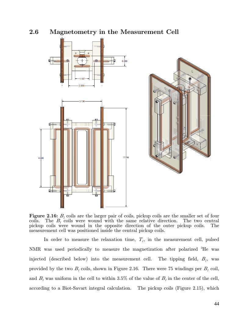
44

2.6 Magnetometry in the Measurement Cell

Figure 2.16: B1 coils are the larger pair of coils, pickup coils are the smaller set of four coils. The B1 coils were wound with the same relative direction. The two central pickup coils were wound in the opposite direction of the outer pickup coils. The measurement cell was positioned inside the central pickup coils.

In order to measure the relaxation time, T1, in the measurement cell, pulsed

NMR was used periodically to measure the magnetization after polarized 3He was

injected (described below) into the measurement cell. The tipping field, B1, was

provided by the two B1 coils, shown in Figure 2.16. There were 75 windings per B1 coil,

and B1 was uniform in the cell to within 3.5% of the value of B1 in the center of the cell,

according to a Biot-Savart integral calculation. The pickup coils (Figure 2.15), which

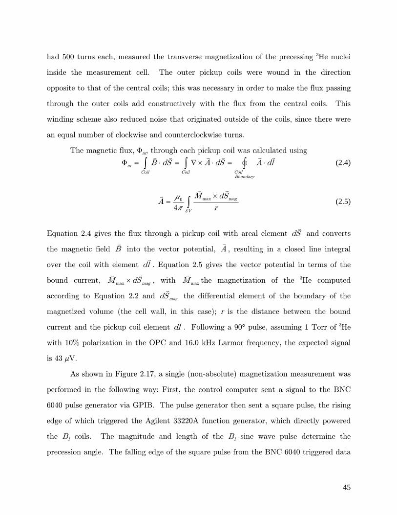
45

had 500 turns each, measured the transverse magnetization of the precessing 3He nuclei

inside the measurement cell. The outer pickup coils were wound in the direction

opposite to that of the central coils; this was necessary in order to make the flux passing

through the outer coils add constructively with the flux from the central coils. This

winding scheme also reduced noise that originated outside of the coils, since there were

an equal number of clockwise and counterclockwise turns.

The magnetic flux, Fm, through each pickup coil was calculated using

m

Coil Coil CoilBoundary

B dS A dS A dlF

(2.4)

max0

4

mag

V

M dSA

r

mp d

(2.5)

Equation 2.4 gives the flux through a pickup coil with areal element dS and converts

the magnetic field B

into the vector potential, A, resulting in a closed line integral

over the coil with element dl. Equation 2.5 gives the vector potential in terms of the

bound current,

max magM dS , with

maxM the magnetization of the 3He computed

according to Equation 2.2 and magdS

the differential element of the boundary of the

magnetized volume (the cell wall, in this case); r is the distance between the bound

current and the pickup coil element dl. Following a 90° pulse, assuming 1 Torr of 3He

with 10% polarization in the OPC and 16.0 kHz Larmor frequency, the expected signal

is 43 mV.

As shown in Figure 2.17, a single (non-absolute) magnetization measurement was

performed in the following way: First, the control computer sent a signal to the BNC

6040 pulse generator via GPIB. The pulse generator then sent a square pulse, the rising

edge of which triggered the Agilent 33220A function generator, which directly powered

the B1 coils. The magnitude and length of the B1 sine wave pulse determine the

precession angle. The falling edge of the square pulse from the BNC 6040 triggered data

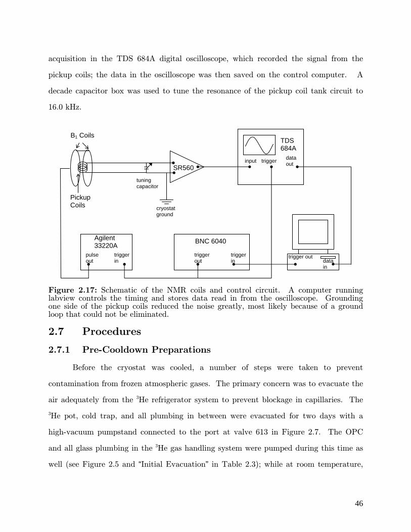
46

acquisition in the TDS 684A digital oscilloscope, which recorded the signal from the

pickup coils; the data in the oscilloscope was then saved on the control computer. A

decade capacitor box was used to tune the resonance of the pickup coil tank circuit to

16.0 kHz.

Figure 2.17: Schematic of the NMR coils and control circuit. A computer running labview controls the timing and stores data read in from the oscilloscope. Grounding one side of the pickup coils reduced the noise greatly, most likely because of a ground loop that could not be eliminated.

2.7 Procedures

2.7.1 Pre-Cooldown Preparations

Before the cryostat was cooled, a number of steps were taken to prevent

contamination from frozen atmospheric gases. The primary concern was to evacuate the

air adequately from the 3He refrigerator system to prevent blockage in capillaries. The

3He pot, cold trap, and all plumbing in between were evacuated for two days with a

high-vacuum pumpstand connected to the port at valve 613 in Figure 2.7. The OPC

and all glass plumbing in the 3He gas handling system were pumped during this time as

well (see Figure 2.5 and “Initial Evacuation” in Table 2.3); while at room temperature,

SR560

TDS 684A

BNC 6040

trigger

Agilent 33220A

Pickup Coils

B1 Coils

input

trigger out

data out

data in

trigger out trigger in

trigger in

pulse out

tuning capacitor

cryostat ground

47

the measurement cell (Figure 2.5) remained isolated and full of air to reduce the

diffusion of plastic vapor from the measurement cell area into the borosilicate plumbing

between the 4.2 K anchor and the OPC. Just before the liquid nitrogen fill, this volume

was evacuated and the 4He pot was pressurized with 7 PSI 4He gas in order to prevent

the pot (which receives its liquid 4He from a porous plug in the storage dewar, Figure

2.6) from filling with liquid nitrogen, which would otherwise freeze during the

subsequent liquid 4He fill. The vacuum vessel (Figure 2.6) was also evacuated with a

high-vacuum pumpstand at this time, in order to prevent the accumulation of ice that

could impede gas flow later.

2.7.2 77 K Procedures

After the cryostat dewar was filled with liquid nitrogen, the vacuum vessel was

filled with ~1 Torr of 4He gas to facilitate the cooling of the cell; in a vacuum this

process could take days. As the measurement cell (and most of the tube between the

measurement cell and the OPC) cooled, the plastic vapor outgassing from the

measurement cell region ceased and cleaning of the OPC could commence. The first

stage of this cleaning was to pump the cell, with valves in the same state as the “Initial

Evacuation” in Table 2.3, for at least 2 days continuously. After this, the cell was filled

with 1 Torr of 4He gas and a bright RF discharge was run in the OPC, with valves in

the “Discharge Cleaning” configuration described in Table 2.3.

The quality of this discharge determined whether further cleaning was required; a

contaminated discharge would reduce the metastable population and therefore the 3He

polarization. A pure helium discharge had distinct emission lines when viewed through

a spectroscope, while a broad continuous spectrum indicated contamination with

molecular gases (such as atmospheric gases or plastic vapor). The discharge quality was

also evaluated using the photodiode, as shown in Figure 2.3. If the signal observed in

the photodiode decreased over time, this indicated the buildup of contaminants in the

48

gas, either from outgassing or the rapid removal of contaminants from the OPC walls

due to the discharge plasma. In this case, the cell was evacuated for another 24 hours

and then the discharge test was performed again. If the photodiode signal increased

with time, this indicated that contaminants were leaving the helium gas, presumably

these contaminants were leaving the OPC walls and landing in some colder area

allowing the discharge to improve. This process of evacuate, fill and test would be

performed until an adequately (adequate here means that fluorescence peaks are clearly

discernible) clean discharge could be run continuously for hours at a time. A week

between the initial liquid nitrogen fill and the first adequate discharge was typical.

Once the OPC was cleaned, the entire cell insert, that is, with OPC open to the

measurement cell, was filled with 1 Torr of 3He (“77 K Optical Pumping”, Table 2.3) in

order to perform initial NMR measurements. Although relaxation measurements at 77

K were not intrinsically important, they were performed because they allowed a final

check of the NMR coils and circuits, as well as optimization of the gradient coil current,

before cooling the cryostat with liquid 4He. In this configuration effectively the entire

cell was optically pumped (for roughly 5 minutes), as the spin-polarized 3He diffused

into the measurement cell and reached an equilibrium polarization. The B1 coils were

calibrated roughly by searching for the pulse magnitude that would maximize the signal

and completely depolarize the measurement cell; a more accurate calibration was

performed later with superfluid in the cell as described in Section 2.7.3. T2 was

measured using the sequence shown in Figure 2.18. p/6 pulses were typically employed

because they produced a large signal while allowing several Free Induction Decay (FID)

measurements before it was necessary to repolarize the gas – the change in

magnetization per pulse was 0 cos 6 1 13%zM M p . It was necessary to cease

optical pumping during all FID measurements since the RF discharge produced

intractable levels of noise in the pickup. The current in the gradient coil (Figure 2.10)

was varied between pulses in order to find the current which maximized T2, typically 5 s

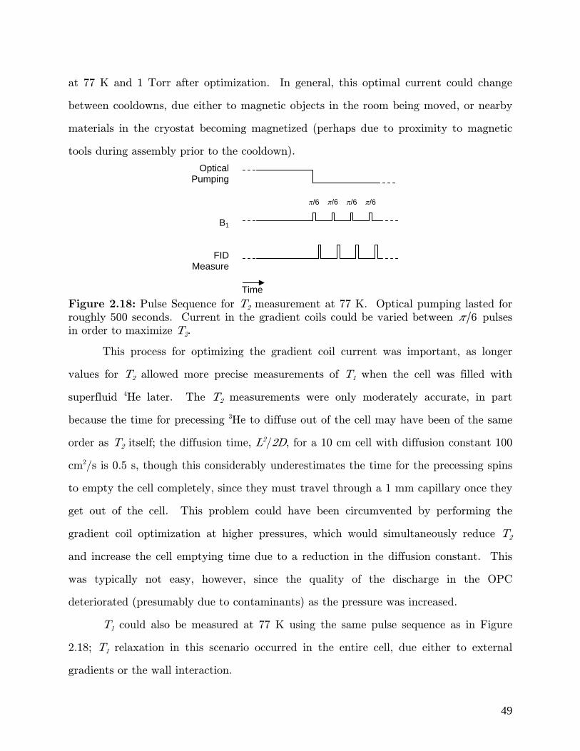
49

at 77 K and 1 Torr after optimization. In general, this optimal current could change

between cooldowns, due either to magnetic objects in the room being moved, or nearby

materials in the cryostat becoming magnetized (perhaps due to proximity to magnetic

tools during assembly prior to the cooldown).

Figure 2.18: Pulse Sequence for T2 measurement at 77 K. Optical pumping lasted for

roughly 500 seconds. Current in the gradient coils could be varied between 6p pulses

in order to maximize T2.

This process for optimizing the gradient coil current was important, as longer

values for T2 allowed more precise measurements of T1 when the cell was filled with

superfluid 4He later. The T2 measurements were only moderately accurate, in part

because the time for precessing 3He to diffuse out of the cell may have been of the same

order as T2 itself; the diffusion time, L2/2D, for a 10 cm cell with diffusion constant 100

cm2/s is 0.5 s, though this considerably underestimates the time for the precessing spins

to empty the cell completely, since they must travel through a 1 mm capillary once they

get out of the cell. This problem could have been circumvented by performing the

gradient coil optimization at higher pressures, which would simultaneously reduce T2

and increase the cell emptying time due to a reduction in the diffusion constant. This

was typically not easy, however, since the quality of the discharge in the OPC

deteriorated (presumably due to contaminants) as the pressure was increased.

T1 could also be measured at 77 K using the same pulse sequence as in Figure

2.18; T1 relaxation in this scenario occurred in the entire cell, due either to external

gradients or the wall interaction.

Optical Pumping

B1

FID Measure

p/6 p/6 p/6 p/6

Time

50

2.7.3 Relaxation Measurements Below 4.2 K

After all 77 K measurements were finished, the remaining liquid nitrogen was

evaporated from the dewar by means of a heater on the bottom of the vacuum vessel.

The dewar was then filled with liquid 4He; the exchange gas remained in the vacuum

vessel to facilitate cooling the cell and refrigerator components inside the vacuum vessel.

When the cell cooled to 4.2 K, the exchange gas was removed with a high vacuum pump

in order to allow operation of the refrigerators. A small amount of exchange gas

probably remained, at a pressure, determined by the ultimate vacuum of the pump,

roughly 10-6 Torr.

In order to perform T1 measurements with polarized 3He in superfluid 4He, the

cell was first filled with liquid 4He. This was accomplished by adding 4He gas to the

measurement cell through the polarized 3He gas system and liquefying it. The 4He gas

was liquefied in the measurement cell with the 4He refrigerator by pumping the 4He pot

and letting 3He into the 3He pot (Figure 2.6). The 3He liquefied in the 3He pot,

effectively improving the thermal connection between the cell and the 4He pot. In order

to fill the measurement cell, the 4He gas was added to the cell incrementally, since the

calibrated volumes could not hold enough 4He gas to fill the cell all at once. The 4He

calibrated volume (Figure 2.5, “4He Cal. Vol. Filling”, Table 2.4) was filled to ~760 Torr,

then allowed into the measurement cell through the getter (“IT L4He MC Filling”, Table

2.3). The fill was stopped when the calibrated volume pressure reached roughly ~100

Torr; then the calibrated volume was refilled and opened to the measurement cell until

the measurement cell was filled to the top of the dTPB coated region, fine tuning the

calibrated volume pressure to the necessary amount on the final fill. Once the

measurement cell was filled, it was allowed to cool to 1.5 K or below before starting the

3He refrigerator. Since the 3He refrigerator was pumped by both a turbo pump and

backing pump, two modes of operation were possible (Figure 2.7): it was possible to

pump the 3He pot with only the backing pump, or with both the turbo pump and the

51

backing pump. With just the backing pump, the cell generally reached temperatures

between 550 mK and 700 mK. With the turbo pump also running, the cell reached

temperatures of 400 mK to 500 mK. The choice of pumping configuration was the only

way that the measurement cell temperature was controlled during the measurements.

Once the measurement cell reached its ultimate temperature, a simple method,

hereafter called the injection technique, was used to introduce polarized 3He. First, the

OPC was filled with 1-4 Torr 3He gas (“IT 3He OPC Filling” Table 2.3) and optically

pumped for 10-45 s (“IT 3He Optical Pumping”, Table 2.3), with longer pumping times

corresponding to higher cell pressures. Second, after the optical pumping, the valves

between the OPC and measurement cell were opened and the 3He gas flowed to the

measurement cell (“IT 3He MC Injection”, Table 2.3). The superfluid film and vapor

flow effect described in Sections 2.1 and 2.4 created a pressure gradient within the

capillary above the measurement cell, which compressed the incoming 3He gas into the

measurement cell, where the 3He went into solution. The injection technique was

typically repeated one or two times prior to beginning a T1 measurement, in order to

achieve a large FID signal. The T1 measurement sequence was then performed, as

shown in Figure 2.19. The magnitude and timing of the B1 pulses were chosen so that

the majority of polarization loss was due to relaxation in the measurement cell rather

than due to the pulses. Figure 2.18 shows a pulse magnitude of p/16 (11.25˚), but

pulse magnitudes ranged from 10˚ to 15˚, with corresponding polarization losses of

1.6% to 3.4% per pulse.

The T1 measurement ended when either the height of the FFT peak

corresponding to the Larmor frequency, which was calculated automatically after a FID

signal was acquired, was less than twice the background, or after the same Larmor peak

had decreased by a factor of 10 from its initial value. From this point, more polarized

3He could be injected into the measurement cell and more T1 measurements could be

performed. Eventually the concentration of 3He became high enough that concentration

52

effects became potentially significant (this will be discuused in detail in the next

chapter); at this point, the measurement cell was evacuated by pumping the overnight

in the configuration given by the “Initial Evacuation” row in Table 2.3.

Figure 2.19: Typical sequence diagram for measuring T1 using the Injection Technique.

Peaks in the “4He Storage Pres.” trace correspond to the process of filling the measurement cell with liquid 4He. The first double slash shows the break in time

between the end of the liquid 4He fill and the 3He injections. The pulses in the “Optical

Pumping” and “OPC 3He Pres.” traces correspond filling the OPC, polarizing the 3He

gas, and injecting the polarized gas into the measurement cell. Pulses on the “B1” and

“FID Measure” traces correspond to the T1 measurement sequence Additional injections and T1 measurements (after the second double slash mark) may follow the first, after which the cell is completely evacuated.

The injection technique was utilized to calibrate the B1 coils; a measurement

sequence very similar to the T1 sequence was used, the key difference being that the

timing and pulse magnitude were chosen so that most of the depolarization in the

measurement cell was due to the pulses rather than wall depolarization. To that end, a

tipping angle of p/4 or greater was used instead of the small angle used in the T1

sequence, and the separation of the B1 pulses was approximately 3 s, so that relaxation

from the wall (T1 of order 1000 s) could be neglected. The amplitude of the FID signals

following the pulses should decay according to the rule

1 0cos cosn

n t n tA A Aq q (2.6)

4He Storage Pres.

Optical Pumping

OPC 3He Pres.

B1

FID Measure

p/16 p/16 p/16

Time

53

so that a fit of the signal amplitude vs. pulse number would yield qt. The calibration

data further discussion are found in Appendix A.

54

3 Results

The ultimate goal of the analysis below is to determine Pd at 0.45 K (the

expected operating temperature of the nEDM experiment) and very low x3 since nEDM

will take place at a concentration roughly 7 orders of magnitude lower than used in this

experiment. This was accomplished first by extracting the FID amplitude, which is

proportional to the polarization in the measurement cell, from the raw FID data. An

exponential curve was then fit to the FID amplitude vs. measurement time for each T1

measurement. Finally, EDM 1 3 1,EDM1 0, 0.45 K 1T x T TG was determined

and used to compute Pd for each of the materials.

3.1 Raw Data

The NMR data collected during T1 measurements consisted of 15,000 data point

FID records, sampled at 100 kHz. As described in Section 2.7.3, the FID signal was a

decaying sinusoid, the amplitude of which was proportional to the magnetization of the

polarized 3He in the measurement cell. Figure 3.1 shows two example signals on two

different time scales, the first a FID with zero magnetization in the measurement cell

(the background) and the second with typical magnetization in the measurement cell

after a 12 degree pulse.

55

Figure 3.1: Typical background and FID signals. (a) and (b) show the background and FID signals over the entire measurement interval; (c) and (d) show the background and FID signals in the first millisecond of the measurement.

Several features are immediately apparent from the plots shown in Figure 3.1; the

FID signal decays with lifetime ~100 ms, the Signal to Noise Ratio (SNR) appears to be

~3, and the background noise appears to have a large sinusoidal component. A Fast

Fourier Transform (FFT) of the same data (Figure 3.2) reveals more pertinent

information about the nature of the signals. The peak in the background FFT spectrum

at 16 kHz (the Larmor frequency) corresponds to the resonance of the pickup coils,

while a second peak near 24 kHz mostly resulted from noise from the B0 magnet power

supply, transmitted by the B0 coils.

56

Figure 3.2: FFTs of the background and FID signals shown in Figure 3.1, shown on a semi-logarithmic scale. (a) and (b) show the full FFT spectrum for the background and FID respectively; (c) and (d) show the FFT spectrum in the vicinity of the Larmor frequency for the background and FID measurements. The SNR is roughly 20 for this particular FID FFT.

The SNR in the Fourier spectrum is more important than that in the time

domain, since spectral noise plays the dominant role in altering the best fit to the FID

signal, as discussed below. For the FID FFT in Figure 3.2, the SNR is approximately

20, much larger than in the time domain.

3.2 FID Curve Fits

The magnetization was determined by fitting exponentially decaying sinusoids to

the FID data. A curve of the form in Equation 3.1 was fit to the FID data, accounting

for the signal phase with the relative amplitudes of the sine and cosine parts; the overall

signal amplitude, A, was given by Equation 3.2. This form was chosen rather than a

single sinusoid with a phase term because the phase had a tendency to become unstable

during fits. Fits were performed allowing T2 to vary, then repeated with a fixed value

for T2 (determined from the amplitude-weighted average of T2 fit values). This resulted

57

in more precise values for the FID fit amplitudes, and is justifiable since T2 decay

primarily results from long range gradients, which remain constant over the course of a

T1 measurement. 2/( ) cos 2 sin 2 t T

L LS t a f t b f t ep p (3.1)

2 2A a b (3.2)

FID data were fit using the NonlinearModelFit function in Mathematica 7, which

employed a Levenberg-Marquardt [84] routine. In general, it is not possible to estimate

the uncertainty of the amplitude terms in Equation 3.1 if there is significant spectral

noise near the Larmor frequency; if a sinusoidal noise term, in phase with the FID

signal, is added to the data, then the best fit for a, b and T2 will be altered without

significantly affecting c2/dof, making it impossible for NonlinearModelFit to estimate

the effect of the sinusoidal noise. In reality, the noise did not contain a steady

sinusoidal component near the Larmor frequency, but did contain many transient

spectral components that nonetheless could alter the best fit values. The importance of

these spectral components can be seen by adding a simulated signal to a noise data set

such as that in Figure 3.1a; spectral noise (as opposed to Gaussian distributed noise) is

indicated if altering the phase of the simulated signal results in a clear sinusoidal

dependence of the best fit amplitude on the phase of the simulated signal. Figure 3.3

shows the results of the simulation; the best fit amplitude oscillates sinsuoidally around

the mean best fit amplitude, which is equal to the simulated signal amplitude of 0.4 V.

If the dominant contribution to the fit uncertainty were Gaussian, no such phase

dependence would be evident.

58

Figure 3.3: Total amplitude of the best fit plotted versus the phase of a 0.4 V, 16 kHz simulated FID signal added to a measured background signal. The sinusoidal dependence on the phase indicates that spectral noise plays the most important role in the uncertainty of the fit.

It is important to know how consistent the noise is for each FID measurement; if

there is substantial variation in the noise, it will be difficult to estimate the uncertainty

in the fits. Figure 3.4 shows the result of adding a simulated signal (with variable

phase) to four different noise data sets. Instead of plotting the best fit amplitude versus

the simulated signal phase, the plots show the rms deviation of the best fit amplitude

over a phase range of 2p; for a sinusoidal plot such as in Figure 3.3, the rms deviation is

2 2 times the amplitude of the sine wave.

59

0

0.003

0.006

0.009

0.012

0.015

15984 15986 15988 15990 15992 15994 15996 15998 16000 16002

Simulated Signal Frequency (Hz)

Fit

Am

plitu

de R

MS

Dev

. (V

)1st noise file

2nd noise file

3rd noise file

4th noise file

Figure 3.4: Plot of the RMS deviation in best fit amplitude versus simulated signal frequency using four different noise data sets.

The variation between the plots in Figure 3.4 show that is difficult to determine

confidence intervals for a given FID fit; because of this, the variance from the individual

FID fits could not be determined in order to weight FID fit amplitudes used in the

exponential T1 decay fits. However, a generic FID amplitude uncertainty of 8 mV, the

average of the RMS deviations in Figure 3.4, was useful for testing the T1 fits.

3.3 T1 Fit Technique

An exponential decay curve was fit to the FID amplitudes vs. measurement time.

Figure 3.5 shows a plot of FID fit amplitude vs. measurement time for a typical T1

measurement (Torlon rod in cell). The fit in Figure 3.5 ignores the first FID amplitudes

based on physical considerations which are discussed below.

60

0

0.1

0.2

0.3

0.4

0.5

0.6

0.7

0.8

0.9

1

0 100 200 300 400 500 600

Measurement Time (s)

FID

Fit

Am

plit

ud

e (V

)

Figure 3.5: FID Fit Amplitude vs. measurement time, shown with an exponential decay fit and 8 mV error bars. The first two points were cut from the fit on physical grounds.

3.3.1 Thermal Settling

We expect that in general T1 may depend on the temperature of the cell wall, so

the temperature of the cell should be stable over the measurement interval of the data

to be included. The injection of 3He into the cell results in heating due to the heat of

solution, W, of 3He in liquid 4He, with 1 54 . KBW k [85]. The relationship between

the temperature of the 4He before (T0) and after (Tf) the 3He injection depends on the

molar heat capacity of the 4He, Cp(T), the number of 3He atoms injected, N3, and the

number of moles of liquid 4He present, n4, according to Equation 3.3, which ignores the

heat capacity of the cell since it is small [86,87] compared to that of the liquid 4He.

0

3 4

fT

p

B A T

W RE N n C T dT

k ND (3.3)

Making use of the fact that 3 AN N is the number of moles of 3He, the increase in

temperature is simply related to the change in concentration of 3He x3;

61

0

3

fT

p

BT

WC T dT R x

k (3.4)

Cp for liquid 4He has been thoroughly measured [87], so the change in temperature for an

injection is easily computed. A typical sequence with 43 2 10x and 0 0 45 . KT

should result in a final temperature of 0.63 K. Figure 3.6 below shows the temperature

measured in the cell after a typical injection sequence.

0.4

0.45

0.5

0.55

0.6

-600 -400 -200 0 200 400 600 800 1000 1200 1400 1600

Time After Final Injection (s)

Low

er

Ce

ll T

em

pe

ratu

re (

K)

Figure 3.6: Measurement cell temperature vs. time during a typical injection sequence,

43 2 10xD .

The NMR measurement sequence was started within 30 seconds of the last

injection, typically. Since the cell temperature was recorded during the T1 sequence,

this record can be used to determine which FID data should be cut from the T1

estimate. The equilibration condition of 1thermeqT t c T was employed, with

0.10c (see Section 3.3.3) and T the value of the cell temperature at the end of

the T1 sequence and tthermeq the thermal equilibration time.

62

3.3.2 Liquid 4He Volume

The rate of longitudinal relaxation in the film is non-zero. Since the 3He vapor

above the bulk liquid 4He is in equilibrium with both the bulk liquid 4He and the

superfluid 4He film, which coated the cell above the bulk, the concentration of 3He in the

film should be the same in the film and the bulk. Assuming this is the case, the surface

area from Equation 1.18 is in fact the entire cell surface area that is in contact with

either film or bulk liquid 4He, while the volume is the volume of the bulk liquid. The

Ph.D. dissertation [88] of Q. Ye confirms this hypothesis using an apparatus and

method very similar to that used for this experiment. Figure 3.7 shows plots of the

relaxation rate versus the surface to volume ratio, computed using either the total cell

surface area (Figure 3.7c) or the surface area of the bulk liquid in contact with the cell

(Figure 3.7b); the negative intercept found by using the latter method to compute the

surface area suggests substantial relaxation is occurring outside of the bulk. This has

two implications for the analysis of the Illinois results: First, when computing Pd for d-

TPB, the relaxation on other surfaces must be considered. Second, great care must be

taken in analyzing relaxation measurements with different liquid 4He volumes. The cell

used by Q. Ye [88] was thermally anchored with solid copper wire all along the outside

of the cell, which produced uniform temperatures in the bulk and in the film. The

Illinois measurement cell, however, was anchored at the top and bottom only, which

could have allowed warmer temperatures in the film if a substantial amount of helium

gas was in the vacuum vessel, either due to a leak or exchange gas that was not fully

removed. The parts of the Illinois measurement cell covered by bulk liquid 4He were

thermalized to the lower anchor because of the very high thermal conductivity of

superfluid 4He [83]. Such a temperature difference could alter the clean volume

dependence seen in [88], and therefore make comparison of relaxation results at different

liquid 4He fill levels difficult. Because of this, only cells filled to the same height in the

cell were evaluated; 14.3 cm3 of liquid in the empty cell or 12.25 cm3 if a rod is present

63

(since the rod displaced 2.2 cm3). These fill heights were not identical, but the

difference in film covered areas as a result of the different liquid heights was less than

1% (Figure 2.9).

Figure 3.7: Results of T1 measurements with different amounts of liquid 4He in d-TPB cell, from the Ph.D. Thesis of Qiang Ye [83]. (a)T1 vs. total 4He in cell. (b) T1 vs. surface to volume ratio, using the area in contact with the bulk liquid for S. (c) T1 vs. surface to volume ratio, using the total area of the cell for S.

3.3.3 Diffusion Effects Polarized 3He entered the liquid 4He at the top of the bulk liquid, then spread

throughout the cell by diffusion. According to [89], the diffusion constant of 3He in

liquid 4He at 0.5 K is roughly 1 43

2 -110 cm sx for concentrations in the range used in

this experiment. The diffusion time for an unbounded diffusive medium is simply

(a) (b)

(c)

64

2

2D

Rt

D (3.5)

Using a length of 7.5 cm and x3 of 310 , Equation 3.5 yields a rough estimate of

300 s for the diffusion time. This time is not insignificant compared to the typical

relaxation times of 500-3500 which were measured, so it is important to understand

exactly how the diffusion of polarized 3He throughout the liquid 4He occurred. If the

diffusion time was significant compared to T1, the 3He distribution was weighted toward

upper surfaces of the cell more than lower surfaces, since the polarized 3He enters

solution at the top of the cell; if these surfaces had different Pd, then T1 decay fits will

be affected.

The distribution of polarized 3He concentration, j, after it was injected into the

bulk liquid can be approximated by solving the diffusion equation in one dimension:

( , )D s t zt z z

j (3.6)

0

0,z z Lz

j

(3.7)

0( , ) k kk

s t z L a z t td d (3.8)

Equation 3.6 is the diffusion equation in one dimension with a source term, Equation 3.7

gives the wall reflection boundary condition and Equation 3.8 describes the idealized

source term, which models the polarized 3He injections that entered the liquid at 0z .

The diffusion constant depended on the total 3He (polarized and unpolarized)

concentration, and therefore was not constant throughout the cell after the injection.

When Equations 3.6 – 3.8 were solved numerically, the delta functions in

Equation 3.8 were replaced with finite Gaussians, necessitating the move of the source

terms slightly away from 0z , due to the finite width of the delta function

approximation. The injection sequence modeled was a set of three injections at tk at 0,

65

50, and 100 s with 410ka cm-3; this was a typical sequence, though smaller and larger

injections were also done. The evolution of j(z,t) was determined using different initial

concentrations of unpolarized 3He and a temperature of 0.5 K.

The polarized 3He distribution was considered equalized when the RMS deviation

of the concentration reached 10 percent of the mean value of the concentration,

according to Equation 3.9:

2

1

( )10.1

1

Ni diffusioneq

i

x t x

x N

(3.9)

with xi the concentration at equally spaced intervals in the cell and tdiffusioneq the diffusion

equilibration time, which was used as cut criteria in the T1 fits. The diffusion

equilibration time was roughly proportional to the initial concentration, as shown in

Figure 3.8.

Figure 3.8: (a) shows the polarized 3He equilibration time vs. the initial total 3He concentration after a typical injection sequence. (b) shows the polarized 3He concentration, divided by the average concentration, vs. distance below the liquid

surface at the equilibration time for 4

3 5 10x .

10

100

1000

10000

0.00001 0.0001 0.001 0.01 0.1

Concentration

Eq

uili

bra

tio

n T

ime

(s

)

0.85

0.9

0.95

1

1.05

1.1

1.15

0 0.5 1 1.5 2 2.5 3 3.5 4 4.5 5 5.5 6 6.5 7 7.5

Position (cm)

Re

lati

ve

Co

nc

en

tra

tio

n

(b) (a)

66

3.4 T1 Fit Results

T1 was estimated from the FID fits, employing cuts that were informed by the

physical effects discussed above. The appropriateness of the thermal settling cuts were

evaluated for the empty cell data, based on the change in c2/dof for different thermal

settling parameters. The results presented below include a correction for the B1 pulse

depolarization, described in detail in Appendix A.

3.4.1 Empty Cell The relaxation time in the empty cell (that is, without a sample rod present but

filled with liquid 4He) was used to compute depolarization probabilities both for d-TPB

and for all the sample rods as well, so the determination of T1 for the empty cell was

vital for all materials. T1 was the longest in the empty cell measurements, roughly 3000

seconds, making it the best data for evaluating the validity of cuts based on the

considerations discussed in the previous section. The cut criteria were determined from

the diffusion and thermal equilibration times,

Max ,cut thermaleq diffusioneqt t t (3.10)

All FIDs measured before tcut were eliminated from the T1 fit. c2/dof was

evaluated for the empty cell T1 fits using different values of the thermal equilibration

parameter. It is evident from Figure 3.9 that the 8 mV uncertainty for the FID fit

amplitudes was not always correct for the FIDs since c2/dof varied over such a wide

range for the different T1 measurements. Most likely, this was due to variations in the

FID background. Because of the wide range of c2/dof for the T1 fits, the geometric

mean was used to evaluate the effect of different thermal equilibration parameter values.

The particular value of the equilibration parameter had very little impact on the

geometric mean of c2/dof (Table 3.1), so a value of 10 percent for the cutoff parameter

was chosen in order to keep a large amount of data for the fits.

67

Thermal Equilibration parameter

c2/dof Geometric Mean

0.05 1.109 0.10 1.046 0.20 1.05

Table 3.1: Geometric mean of c2/dof for the empty cell data. Altering the thermal

equilibration parameter altered c2/dof only slightly.

Figure 3.9: (a) c2/dof for each of the empty cell T1 fits plotted vs. the measurement date. (b) Histogram of the empty cell T1 fit residuals, with standard deviation of 9.6 mV.

A histogram (Figure 3.9b) of the empty cell T1 fit residuals shows an

approximately Gaussian distribution with standard deviation 9.6 mV, similar to the 8

mV FID uncertainty determined from the noise data sets. The histogram contains an

excess of counts beyond the 3s level, however, so the Gaussian distribution is only

approximate. The NonlinearModelFit routine in Mathematica estimates fit

uncertainties accurately when the noise is normally distributed [90], so this technique

was used to generate error bars (1s) for all of the T1 fits, despite the modified

distribution measured.

Figure 3.10 shows the T1 fits for the empty cell, plotted vs. different physical

variables. The plot in (b) shows a clear x3 dependence, necessitating the use of low x3

data (since T1 was relatively constant for low x3) when examining other trends in T1.

There was also a time dependence in T1, probably due to a degradation of the cell

68

surface, which was best fit with a Heaviside step function plus a constant as shown in

(e). The depth of the step was 270 s; this amount was added to the fits in (c) and (d)

after the step in order to cancel the time dependence, resulting in much smoother plots.

Figure 3.10: (a) T1 vs. cell temperature at low concentrations. (b) T1 vs. x3. (c) T1 vs. cell temperature after the time dependence was corrected. (d) T1 vs. x3 after the time dependence was corrected. (e) T1 vs. measurement date for low concentrations.

Since T1 did not appear to depend on temperature,

Empty Cell 4 1

EDM 1 31 0 3.67 0.02 10 sT xG was determined from a straight line

fit of T1 vs. x3 (Figure 3.10d) for the d-TPB Pd calculation. Empty Cell

EDMG was computed in

2500

2600

2700

2800

2900

3000

5/27 5/28 5/29 5/30 5/31 6/1 6/2 6/3 6/4

Date

T1

(s)

Heaviside

x3 < 0.0012

2500

2600

2700

2800

2900

3000

0.4 0.45 0.5 0.55 0.6 0.65

Cell Temp (K)

T1

(s)

2400

2500

2600

2700

2800

2900

3000

3100

3200

3300

3400

0 0.001 0.002 0.003 0.004 0.005 0.006 0.007 0.008 0.009 0.01

x3

T1 (

s)

x3 < 0.0012

2500

2600

2700

2800

2900

3000

0.4 0.45 0.5 0.55 0.6 0.65

Cell Temp (K)

T1

(s)

x3 < 0.0012, Time Dependence Removed

2600

2800

3000

3200

3400

3600

3800

4000

0 0.001 0.002 0.003 0.004 0.005 0.006 0.007 0.008 0.009 0.01

x3

T1

(s)

x3 < 0.0012, Time Dependence Removed

(a) (b)

(d) (c)

(e)

69

a different way for the rod Pd calculations, however, since the dominant uncertainty was

from the step-like drop in relaxation times that occurred around May 30, 2009 (Figure

3.10e) rather than any statistical uncertainties in the T1 measurements. Whether this

drop was permanent depends on the reason for it; if, for example, the drop in T1 was

due to contamination with paramagnetic O2 (due to a leak), it is likely that this gas left

the cell after the cell was warmed up to room temperature. If the drop was due to a

contaminant that is solid at room temperature, then it should be permanent; this seems

unlikely, however, as there were no loose materials within the cell. However, if

hydrocarbons (pump oil, e.g.) landed in the measurement cell, this might have altered

the relaxation time permanently since this might not have evaporated after a warmup.

It is not possible to determine whether the decrease in T1 was permanent, so for

the rod Pd calculations, T1 at low concentration and 0.45 K was determined by taking

the mean of T1 before and after the step (Figure 3.10e), with uncertainty equal to half

the difference between the steps;

Empty Cell

1,EDM 2700 140 sT (3.11)

EDM

Empty Cell 4 13.70 0.20 10 sG (3.12)

3.4.2 Bare Torlon Sample Rod

T1 was measured with the bare Torlon rod in the measurement cell (Figure 3.11).

At low concentrations, there are small slopes in T1 vs. measurement date and vs. cell

temperature, however, the cell temperature was negatively correlated with the

measurement date (Figure 3.11d). Determining whether the slopes in Figure 3.11a-b are

due to time dependence, temperature dependence, or some combination therefore is not

possible in this case. G at low concentration and 0 45. KT is the quantity that is

relevant for nEDM; assuming the trend in Figure 3.11b is due to temperature

dependence, T1 is given by

1 0 1T A AT (3.13)

70

with 0 1440 70 s, 270 110 s/KA A . This technique for finding Bare Torlon

1,EDMT was

chosen since it is the most pessimistic estimate. Propagating the error (including the substantial covariance),

1,EDM

Bare Torlon 570 20 sT (3.14)

Bare Torlon 3 1

EDM 1.77 0.07 10 sG (3.15)

Figure 3.11: T1 fits for the bare Torlon rod. (a) T1 vs. measurement date for low concentrations. (b) T1 vs. cell temperature for low concentrations. (c) T1 vs. 3He concentration. (d) Cell temperature vs. measurement date.

3.4.3 Coated Torlon Rod

The relaxation time of the Torlon rod in the measurement cell was measured

again after the rod was coated with Pyralin semi-conductor grade resin (Figure 3.12).

While T1 increased dramatically for the coated Torlon rod when compared to the

uncoated rod measurement, these results have a larger uncertainty because the

measurements occurred while the vacuum can was leaking helium gas. This leak

prevented the cell from getting cooler than 0.67 K; in addition to increasing the

temperature of the cell, this leak could have altered relaxation rates in the film; in

400

450

500

550

600

650

700

0.4 0.45 0.5 0.55 0.6 0.65 0.7 0.75

Cell Temp (K)

T1

(s)

400

450

500

550

600

650

700

5/6 5/7 5/8 5/9 5/10 5/11 5/12 5/13 5/14

Measurement Date

T1

(s)

x3 < 0.0012 x3 < 0.0012

0.4

0.45

0.5

0.55

0.6

0.65

0.7

0.75

5/6 5/7 5/8 5/9 5/10 5/11 5/12 5/13 5/14

Measurement Date

Ce

ll T

em

p (

K)

400

450

500

550

600

650

700

0 0.0005 0.001 0.0015 0.002 0.0025

x3

T1

(s)

x3 < 0.0012

(a) (b)

(c) (d)

71

particular, the temperature of the upper cell, which was not covered by bulk liquid or

close to an anchor, could have been substantially warmer than the bulk liquid.

Variations in the vacuum can pressure could be entirely responsible for the time

dependence in Figure 3.12a. The slope in Figure 3.12b is almost certainly not due to

temperature dependence since T1 changed by a substantial amount over a very small

range in cell temperature.

Figure 3.12: T1 fits for the coated Torlon Rod. (a) T1 vs. measurement date for low concentrations. (b) T1 vs. cell temperature for low concentrations. (c) T1 vs. 3He concentration.

Figure 3.12c, while showing no x3 dependence, demonstrates the wide range of T1

values for this measurement. It is not possible to say for certain whether T1 was

increased, decreased, or unaffected by the leak; the wide range of measured T1 values in

Figure 3.12c, however, suggests that some unknown effect was at work. Taking a simple

average of the low concentration data, with uncertainty determined by the range of the

T1 values gives

Coated Torlon

1 3 0, 0.67 K 1300 100 sT x T (3.16)

1150

1200

1250

1300

1350

1400

1450

7/13 7/14 7/14 7/15 7/15 7/16 7/16 7/17 7/17 7/18 7/18

Measurement Date

T1

(s)

1100

1200

1300

1400

1500

1600

0.4 0.45 0.5 0.55 0.6 0.65 0.7 0.75

Cell Temp (K)

T1

(s)

1100

1150

1200

1250

1300

1350

1400

1450

1500

1550

1600

0 0.001 0.002 0.003 0.004 0.005 0.006

x3

T1

(s)

x3 < 0.0012 x3 < 0.0012

(a) (b)

(c)

72

Coated Torlon 3 1

3 0, 0.67 s 0.77 0.06 10 sx TG (3.17)

3.4.4 Coated BeCu Rod

The relaxation times for the Pyralin coated BeCu rod had substantial x3

dependence (Figure 3.13a). T1 vs. concentration was fit with a straight line over the

range it was linear, given by

1 1,0 3T T Kx (3.18)

with 5

1,0 680 17 s, 1.2 0.14 10 sT K . The Kx3 term was subtracted from

the data in order to evaluate temperature and measurement date trends (Figure 3.13b,

3.13c). As with the empty cell test, there was no measured temperature dependence for

T1; unlike the empty cell, there was no apparent dependence on the measurement date.

Figure 3.13: (a) T1 vs. x3 for the coated BeCu rod. (b) T1 vs. Temperature for the coated BeCu rod after the concentration dependent part of the fit from Figure 3.13a was subtracted. (c) T1 vs measurement date after the concentration dependent part of the fit from Figure 3.13a was subtracted.

660

670

680

690

700

710

720

730

740

750

760

0.4 0.45 0.5 0.55 0.6 0.65 0.7 0.75 0.8

Cell Temp (K)

T1

(s)

700

800

900

1000

1100

1200

1300

0 0.001 0.002 0.003 0.004 0.005 0.006 0.007 0.008 0.009

x3

T1

(s)

660

670

680

690

700

710

720

730

740

750

760

6/11 6/12 6/12 6/13 6/13 6/14 6/14

Date

T1

(s)

(a) (b)

(c)

Concentration Dependence Removed

Concentration Dependence Removed

73

Since the concentration dependence is by far the dominant effect on the

relaxation time for the BeCu rod, BeCu

1,EDMT was equated to the zero intercept of the fit in

Figure 3.13a, yielding

BeCu

1,EDM 680 17 sT (3.19)

BeCu 3

EDM 1.47 0.04 10G (3.20)

3.5 Depolarization Probabilities

The depolarization probabilities were calculated using Equation 1.18 and the

values of GEDM calculated above. In the case of the empty cell, there were several

materials present in addition to the d-TPB; namely, 1266 Stycast as well as Pyralin

coated Cu. In order to calculate d-TPB

dP , it is necessary to determine

d-TPB Empty Cell Stycast Coated Cu

EDM EDMG G G G (3.21)

There is relatively little data available on the relaxation of polarized 3He in bulk

liquid, particularly in the presence of metals. It is reasonable, then, to use BeCu

EDMG to

estimate Coated CuG . Since there were 2.5 cm2 of Pyralin coated copper in the empty cell

in the presence of 14.3 cm3 liquid 4He, and 17.0 cm2 of Pyralin coated BeCu copper in

the presence of 12.26 cm3 liquid 4He;

Coated Cu BeCu Empty Cell 3 1

EDM EDM

12.262.5 17.0 0.13 10 s

14.3G G G

(3.22)

The ratio of liquid volumes in Equation 3.22 is due the S/V dependence of G.

Nacher et al. [91] measured 1 1 minT at 100 mK in a cell constructed from 1266

Stycast with 16 cmS V . S V for the Stycast in the measurement cell was

2 3 19.7 cm 14.3 cm 0.68 cm , so naively we expect that

Stycast Stycast 3 1

IL UBC0.68 6 2 10 sG G (3.23)

This relaxation rate far exceeds the total relaxation rate observed in the empty cell.

Since the Nacher measurement was performed at 100 mK, the result is not directly

comparable to the IL result, but it casts serious doubt on our ability to estimate d-TPB

dP .

74

It is noted in [91] that the observed relaxation time for 1266 Stycast was in excess of

what had been observed elsewhere, perhaps due to the difference in storage containers

used in the United States (steel) versus Europe (glass). The 1266 Stycast in the

measurement cell in fact came from a glass container, but this does not remove the

uncertainty about the relaxation rate due to the Stycast. Since it is ultimately not

possible to determine the exact effect of the 1266 Stycast, the depolarization probability

for d-TPB must be left as an inequality, with 3

Empty Cell 14.3 cmV the volume of liquid

4He in the empty cell:

<

1*

d-TPB Empty Cell 7d-TPBEDM

Empty Cell

4 1.32 108

d

B

S mP

V k T

pG

(3.24)

Calculating the depolarization probabilities for the rod materials is more

straightforward:

1

*Empty Cellrod rod Empty Cell rod

EDM EDM

rod rod

48

d

B

V S mP

V V k T

pG G

(3.25)

The depolarization probabilities for the rod materials are given below:

Bare Torlon 61.01 0.08 10dP (3.26)

Coated Torlon 72.5 0.1 10dP (3.27)

Coated BeCu 77.9 0.3 10dP (3.28)

75

4 Conclusions The main purpose of the research described in the preceding pages is to

determine the effect of wall materials on in the planned nEDM apparatus on 3He

relaxation. This is straightforward for estimating T1 in the measurement cell, but will

require some assumptions for the Torlon plumbing, which are discussed below. In

addition, the concentration and temperature trends are interesting in and of themselves,

and are given some further consideration. Finally, some ideas on possible improvements

and future work are discussed.

4.1 Wall Relaxation in nEDM

Polarized 3He will spend roughly 1000 s in the measurement cells in the nEDM

experiment, so this area is the most sensitive to wall depolarization. From the

depolarization probability for d-TPB (Equation 3.23), the surface to volume ratio of the

nEDM cells (0.51 cm-1) and Equation 1.18,

>nEDM cell

1 16,000 sT (4.1)

which is in excess of the design goal of 10,000 s.

Relaxation of polarized 3He in the Torlon plumbing is a serious concern,

especially since Torlon had a substantially higher value for Pd (when uncoated) than d-

TPB. S/V for an open-ended cylinder is simply 22 2RL R L Rp p , or 1.57 cm-1 for a

1” I.D. pipe. Combined with the depolarization probabilities, this leads to

bare torlon 3 1

pipe 1.51 10 sG (4.2)

coated torlon 4 1

pipe 3.72 10 sG (4.3)

76

The exact amount of depolarization depends on how much time the polarized 3He

spends in the plumbing. A 3-D simulation is required to make an accurate estimate of

the depolarization as 3He travels through the pipe, since the relaxation rate will decrease

significantly after 3He enters the measurement cell; however, the unbounded diffusion

time ( 2 / 2R D ) is probably similar to the transit time. The diffusion constant at 0.45

K is roughly 400 cm2/s, and the 2m pipe length can be used for R, yielding a diffusion

time of 50 s. If we assume

Exp DP tG (4.4)

then the polarization fraction after transit through the pipe will be 93% for bare Torlon

and 98% for coated Torlon.

Equation 4.4 overestimates the polarization loss, however, since the rate of

depolarization is proportional to the amount of polarized 3He in the pipe, which

decreases as the 3He exits the pipe. The 7% loss estimated for bare Torlon is not ideal

since it will lead to a large initial noise background during the measurement cycle;

whether this will make a significant impact on the measurement sensitivity must be

calculated. The 2% loss associated with coated Torlon is probably acceptable, but

coating the inside of a 2m long pipe has not been tried yet. In addition, the relaxation

data obtained at Illinois for the coated Torlon is less certain (due to the leak during the

measurement), so a future relaxation measurement with an internally coated pipe is

probably required. A one dimensional simulation of the plumbing, described in

Appendix B, predicted somewhat less depolarization.

A Pyralin coated BeCu bellows will be present in some of the valves, leading to

brief contact by polarized 3He. There was some concern that this material would

depolarize 3He so quickly that a NMR signal would not be observable in tests at Illinois;

the fact that coated BeCu actually outperformed the uncoated Torlon was cause for

relief. 3-D simulation would be required to estimate the depolarization of 3He as it

traveled around the bellows, but since the time of exposure is expected only to be a few

77

seconds (and conductance to the bellows will be limited), it is safe to say that coated

BeCu will not be a concern for 3He polarization in nEDM.

4.2 Concentration and Temperature Effects

There is relatively little published about the relaxation of polarized 3He in bulk

liquid. An experiment in a cell with bulk liquid in the presence of a Nuclepore surface

was performed [92] at temperatures between 27 and 500 mK, but due to the extremely

large S/V of that material, the relaxation time was determined by the time to diffuse to

the Nuclepore surface. Other experiments [93,94] were performed with bulk liquid, but

at temperatures in the vicinity of the lambda point (2.17 K), a totally different regime

because of the relatively small fraction of 3He bound in the liquid 4He, as well as the

rapidly changing properties of liquid 4He at that temperature.

The lack of temperature dependence in T1 (with the possible exception of the

bare Torlon measurements, where the temperature dependence was weak in any case)

was somewhat of a surprise. If there were bound states for 3He on the walls, strong

temperature dependence would be expected, since the time spent in the bound state

should be strongly temperature dependent. On the other hand, if the polarized 3He

simply bounced off the walls, then T1 should have increased as temperature decreased

since the collision rate decreased as well, and the interactions should have become more

adiabatic as the speed of the 3He decreased. In the end however, not much can be said

about the temperature dependence of 3He relaxation since the temperature range

investigated was fairly narrow. In the range from 0.4 K to 0.7 K, however, temperature

did not have a significant effect on relaxation times.

The 3He concentration was quite important for the empty cell and the coated

BeCu rod (but not the Torlon rod, coated or uncoated). There are several factors that

could depend on the concentration. The most obvious is the diffusion time. The cuts

made to account for diffusion time, however argue against this being the cause, unless

78

there was dramatic non-uniformity in the relaxation rates throughout the cell. Another

possibility is that some of the wall relaxation was due to large magnetic impurities,

perhaps from larger pieces of magnetic material in the metal. Relaxation in the vicinity

of these fields might be analogous to the relaxation of a gas in an external gradient

(discussed in Section 1.4.1) which depends on the diffusion constant. In this case, we

would expect the relaxation time to increase (as was observed) as concentration

increases since the decreasing diffusion constant would cause transport in the vicinity of

the impurity to become more adiabatic.

4.3 Future Work

Several more measurements using the current apparatus could be useful for the

nEDM project. The relaxation measurement for coated Torlon should be repeated,

perhaps constructing a new cell from the actual Torlon pipe to be used in the plumbing,

rather than dropping a rod in the cell. A measurement of the relaxation time for a

Stycast rod or d-TPB coated acrylic rod would resolve the ambiguity (due to film

relaxation on 1266 Stycast) in the depolarization probability for d-TPB.

The large amount of film relaxation could be reduced by filling the cell all the

way to the copper v-groove flange above the cell and replacing the large diameter 1266

Stycast piece above the cell with capillary (Figure 2.7). This probably would not affect

relaxation rates significantly, but would reduce ambiguity in the analysis.

The issue of time dependence should be investigated as well. This could be done

by measuring the effect of introducing oxygen into the optical pumping cell and

injecting it into the measurement cell. If enough O2 landed in the measurement cell, it

should have an effect. Warming up the cryostat and pumping it out should cause the

relaxation time to recover if the O2 had an effect.

Measuring relaxation times over a wide range of magnetic fields would also be

useful. This was performed in much earlier tests on a non-deuterated TPB cell without

79

effect, but probably should be repeated at least for the BeCu, which is likelier to have

ferromagnetic impurities, since, in that case the relaxation rate varies inversely with

2

0B .

The analysis could also be carried further. The early time data for the high

concentration empty cell and BeCu measurements could be examined to see if the

relaxation rate changed as the polarized 3He distribution changed. This would indicate

significantly nonuniform relaxation in the measurement cell and might explain the

concentration effect, although further modeling would be necessary to confirm this.

The effect of long ranged magnetic impurities should be calculable in a simple

enough model, either analytically or through simulation. This could lead to useful

information about the range of the fields in the measurement cell; if the range is small

enough, perhaps these fields could be blocked with thicker coatings.

Finally, there are many improvements to the apparatus that could be made.

Reducing the amount of 1266 Stycast in the measurement cell would probably improve

relaxation times. There is also a large amount of 1266 Stycast tubing in the polarized

3He cell plumbing, which was used because of the lower adsorption energy (compared to

pyrex) for 3He. However, much of this tubing is coated with a superfluid 4He film

during the measurement process and thus the adsorption energy is probably not

relevant; all the tubing in the Q. Ye’s apparatus [88] was pyrex without causing any

apparent problems. Replacing this 1266 Stycast with pyrex would reduce the

contamination from outgassing plastic tremendously, allowing the MEOP process to be

performed more efficiently and less time to be devoted to cleaning the cell after the LN2

cooldown.

80

A B1 Coil Calibration The B1 coils were calibrated at least once during each measurement according to

the method outlined in Section 2.7.3; a rapid sequence of large B1 pulses was performed,

and the depolarization per pulse was determined by fitting the amplitude vs. pulse

number with an exponential decay curve; a typical calibration fit is shown in Figure

A.1. The angle inferred from that exponential decay constant determines the

calibration. Table A.1 shows the results of the calibration measurements.

Figure A.1: Fit to typical calibration data, taken May 1st, 2009. 8 mV uncertainty

used to compute c2/dof.

Calibration date Experiment

Pulse (V-

cycles)Angle

(Degrees)Uncertainty (degrees)

Calibration (Degrees / V-cycle)

Uncertainty (Degrees / V-cycle)

05/01/09 Bare Torlon 200 22.79 0.36 0.1140 0.0018

05/01/09 Bare Torlon 450 51.25 0.29 0.1139 0.0006

05/04/09 Bare Torlon 300 33.31 0.36 0.1110 0.0012

05/28/09 Empty Cell 160 18.24 0.70 0.1140 0.0044

06/02/09 Empty Cell 400 48.21 0.27 0.1199 0.0007

06/12/09 BeCu 150 50.05 0.19 0.3323 0.0012

07/15/09 Coated Torlon 140 19.04 0.17 0.1360 0.0012

Table A.1: Results of all the calibration measurements performed. The pulse column refers to the settings of the function generator used to drive the B1 coils.

The most striking detail in the calibration data is the difference between the

BeCu calibration and the others by a factor of 3. This was probably due to eddy

0

0.2

0.4

0.6

0.8

1

1.2

0 1 2 3 4

Pulse Number

FID

Am

plit

ud

e (

V)

q = 52.0 ± 0.3 ° c2/dof = 0.78

81

currents from the conductive BeCu rod, which tend to cancel the B1 field inside the rod

and amplify it outside of the rod. The calibration constant tended to vary between

experiments, but fell within statistical uncertainties when multiple calibrations were

done during the same experiment. The variation between the calibrations taken during

the bare Torlon, empty cell, and coated Torlon measurements were probably due to the

variation in position of the B1 coils, which would affect the B1 field in the cell due to

changes in eddy currents induced in the vacuum can and the 3He pot, which was located

inside of the B1 coils.

The observed value for T1 is altered depending on the magnitude of the B1 pulse

angle, q, since the magnetization evolves according to

1

1 cos t Tn nM M eq D

(A.1)

with cosq the fractional loss in polarization due to the previous B1 pulse and Dt the

measurement interval. Therefore, when Mn vs. measurement time was fit, the best fit

value for T1 was decreased because of the B1 pulse. The relationship between the best

fit value for T1 (which we will refer to as 1T ) and the actual longitudinal relaxation

time T1, is simply

1 1cost T t Te eqD D (A.2)

Taking the natural logarithm of both sides and solving for T1 leads to

1

1 ln cos

tT

t T qD

D

(A.3)

In the limit as 1 10, T Tq as we expect. The uncertainty in T1 due to the

uncertainty in q is given by

2

1 11 2

1

sintan

cosln cos

T t TT

tt T

qd dq dq dq q dq

q qq

DDD

(A.4)

In the case of typical empty cell measurements using a 16° pulse and a measurement

interval of 200 s with T1 of 3000 s, the uncertainty in T1 is 35 s for a calibration

uncertainty of 1%. Table A.2 shows dT1(dq) along with the statistical uncertainties in

T1 from Section 3.4 for each of the different material measurements, assuming 1%

82

calibration uncertainty and using typical values for T1, q, and Dt. Observed statistical

uncertainties were much larger than dT1(dq).

Measurement q (degrees) t (s) T1 (s) T1(dq) (s)dT1 (s)

(Statistical) Empty Cell 14.3 206 2700 35 140

Bare Torlon 13.8 98 570 2 20

Coated Torlon 12.1 150 1300 5 100

BeCu 15.1 150 680 2 17

Table A.2: Uncertainty in T1 due to a 1% uncertainty in the calibration constant and observed statistical uncertainties from Section 3.4.

83

B 3He Transport Simulation

The transport of polarized 3He from the accumulation volume (Figure 1.7) to the

measurement cells will result in some loss of polarization. Since depolarized 3He will

create a background by capturing neutrons, it is important to estimate the loss in

polarization due to transport through the plumbing.

It is necessary to do a three dimensional simulation to estimate the polarization

of 3He in the measurement cells accurately, but the transport process can be

approximated in one dimension. The system includes the pipe, which is 2 m long and

2.54 cm in diameter, and the cells, which are each 7.6 cm by 10.2 cm by 40 cm; the

diffusion constant at 0.45 K is approximately 400 cm2/s [75]. The cells have a much

larger cross-sectional area (the cross section of the smallest face is used in the

calculations below) and therefore a much larger volume per unit length. In order to

model this difference in one dimension, the spatial coordinate, z, and diffusion constant,

D, in the cell region (but not the pipe) are transformed,

z az (B.1)

D cD (B.2)

z is stretched according to Equation B.3 in order to account for the larger volume per

unit length in the cells:

cell

pipe

z Aa

z A

(B.3)

The diffusion equation must be unchanged by the transformation;

2 2

2 2

, ,z t z tD D

z t z

j jj

(B.4)

2 2

2 2 2

, ,z a t z tcD D

z a z

j j

(B.5)

Combining Equations B.3 and B.5 yields

84

2

2 cell

pipe

Ac a

A

(B.6)

The important features of the transformed region are maintained by the

transformations; the volume of the cells is conserved by stretching their length, and the

diffusion time, 2 2L D , in the cells is preserved since 2 1a c , as expected since the

diffusion equation was conserved.

Figure B.1: Plots of 3He concentration j vs. position at three times; the pipe runs from z=0 to 200 cm, the cells run from z=200 to 240 cm. Position is given in the unprimed coordinate.

Applying this transformation to the pipe-cell system, with the ratio of the cell

cross section (both cells) to pipe cross section 30.6, results in a length of 1224 cm

(increased from 40 cm) and a diffusion constant of 5 24 10 cm s in the transformed

system. The diffusion equation was solved numerically using an injection term at

1 st and wall reflection boundary conditions as in Section 3.3.3. Figure B.1 shows

the 3He concentration vs. position at three times. The concentration in the two regions

0

0.5

1

1.5

2

2.5

0 20 40 60 80 100 120 140 160 180 200 220 240

z (cm)

(t

) (A

rb U

nit

s)

0

0.1

0.2

0.3

0.4

0.5

0.6

0.7

0.8

0.9

0 20 40 60 80 100 120 140 160 180 200 220 240

z (cm)

(t

) (A

rb U

nit

s)

0.13

0.14

0.15

0.16

0 20 40 60 80 100 120 140 160 180 200 220 240

z (cm)

(t

) (A

rb U

nit

s)

t=5 s t=35 s

t=150 s

(a) (b)

(c)

85

does not equalize until ~150 s; however, we are concerned with the time for the 3He to

exit the plumbing.

The total amount of 3He, pipeM t , in the pipe is

pipe pipe

0

( ) ,l

M t A z t dzj (B.7)

with 200 cml the length of the pipe. Figure B.2 shows pipeM t vs. time. After 5 st ,

pipeM t was well fit by an exponential decay plus a constant

fit 0empty

Expf ftM t M M MT

(B.8)

with 0 empty226, 24.4, and 37 s.fM M T The final amount of 3He in the pipe,

Mf , is approximately the ratio of the pipe volume to the volume of the cells times M0.

0

20

40

60

80

100

120

140

160

180

200

0 25 50 75 100 125 150

Time (s)

M(t

) (a

rb u

nit

s)

0

20

40

60

80

100

120

140

160

180

200

Figure B.2: Amount of 3He in the Torlon pipe vs time and exponential fit.

The rate of change of the polarization is approximately

fitpipe

0

dP M tMdt

G (B.9)

86

using pipeG for bare and coated Torlon from Section 4.1; relaxation in the measurement

cells is ignored because of their large surface to volume ratio and small Pd This

approximation equates the 3He number density with the polarized 3He concentration, so

it is only valid for 1P . After integrating both sides of Equation B.9, the time

evolution of P is given by

empty

pipe empty0 0

ln ( ) 1 1t Tf fM M

P t T e tM M

G (B.9)

Polarization loss vs. time is plotted for bare and coated Torlon in Figure B.3,

along with the total amount of 3He in the cells, which was determined by subtracting

pipeM t from the total amount of 3He. Most of the 3He will be in the cells after 80 s, so

we assume that the valve to the cell will be closed at this time. The polarization loss

for bare Torlon would be 5.5% at 80 s, and 1.4% for the coated Torlon.

Figure B.3: Polarization loss vs. time for bare and coated Torlon. The fraction of 3He in the cells is also shown, approaching an asymptote at 86%

There are a number of flaws in this model. First, a one dimensional model

cannot account for the real geometry of the system. Second, the relaxation rate is for

the entire system (and only valid for small losses); we actually want to know the

polarization fraction in the cells rather than in the cells and pipe combined. Despite

these shortcomings, however, this model captures the important features of the system

and gives a good qualitative picture of the polarized 3He transfer process.

0

0.01

0.02

0.03

0.04

0.05

0.06

0.07

0.08

0 30 60 90 120 150

Time (s)

Fra

ctio

na

l Po

lari

zatio

n L

oss

0

0.1

0.2

0.3

0.4

0.5

0.6

0.7

0.8

0.9

Fra

ctio

n o

f 3 H

e in

Ce

lls

Bare Torlon

Coated Torlon

Fraction 3He in Cell3He

87

References

[1] C. S. Wu, E. Ambler, R. Hayward, D. Hoppes, and R. Hudson, Physical Review,

105, 1413 (1957)

[2] J. H. Christenson, J. W. Cronin, V. L. Fitch, and R. Turlay, Physical Review Letters

13, 138 (1964)

[3] H. Burkhardt et al., [NA31 Collab.], Phys. Lett. B 206, 169 (1988)

V. Fanti et al., [NA48 Collab.], Phys. Lett. B 465, 335 (1999)

[4] A. Angelopoulos et al. (CPLEAR Collaboration), Phys. Lett. B 444, 43 (1998)

[5] W. M. Yao et al. J. Phys. G, 33, 1, (2006)

[6] A. Alavi-Harati et al., Phys. Rev. Lett., 83, 22 (1999)

[7] Farrar and Shaposhnikov, Phys. Rev. D, 50, 774 (1994)

[8] E. Kolb and M. Turner, The Early Universe, Westview Press, (1994)

[9] F.W. Stecker, Ap. J. 185, 499 (1973); G. Cavallo and R.J. Gould, Nuovo Cimento B

2, 77 (1971)

[10] B.E.J. Pagel, E.A. Simonson, R.J. Terlevich and J. Melnick, Mon. Notes R.

Astron. Soc. 255, 325 (1992)

[11] D. Kunth and W.L.W. Sargent, Astrophys. J. 273, 81 (1993)

[12] J. Yang, M.S. Turner, G. Steigman, D.N. Schramm and K.A. Olive, Astrophys. J.

281, 493 (1984)

[13] P. Bonifacio and P. Molaro, Mon. Notes R. Astron. Soc. 285, 847 (1997)

[14] S.G. Ryan, J.E. Norris and T.C. Beers, Astrophys. J. astro-ph/9903059 (1999a)

88

[15] N. Hata, R.J. Scherrer, G. Steigman, D. Thomas, and T.P. Walker, Ap. J. 458, 637

(1996)

[16] Stergman et al., astro-ph/0603449v2, (2007)

[17] A. D. Sakharov, JETP Lett. 5, 24 (1967)

[18] C symmetry violated in discrepancy between muon and anti-muon decay rates,

University of Liverpool (1957)

[19] Luis Lavoura Gustavo Castelo Branco and Joao Paulo Silva, CP Violation, Oxford

University Press, (1999)

[20] M.V. Romalis et al., Phys. Rev. Lett., 86, 2505 (2001)

[21] R.D. Peccei and Helen Quin, Phys. Rev. Lett, 38, 1440 (1977)

[22] V.A. Rubakov and M.E. Shaposhnikov, Phys. Usp. 39, 461 (1996)

[23] M. Fukugita and T. Yanagida, Phys. Lett. B, 174, 45 (1986)

[24] T. Asaka and M. Shapashnikov, Phys. Lett. B, 620, 17 (2005)

[25] S. Martin, hep-ph/9709356

[26] S. Martin, hep-ph/9709356

[27] S. Dimopoulos, Phys. Rev. D, 24, 1681 (1981)

[28] M. B. Gavela et al., Phys. Lett. 109B, 215 (1982); B. McKellar, S. Choudhury, XG.

He, and S. Pakvasa, Phys. Lett B 197, 556 (1987)

[29] I. B. Khriplovich and A. R. Zhitnitsky, Phys. Lett. 109B, 490 (1982)

[30] S.M. Barr. Int. Journal Mod. Phys. A 8,209 (1993)

[31] Riccardo Barbieri et al, Physics Letters B 369, 283 (1996)

[32] S. Dimopoulos and L. J. Hall, Physics Letters B, 344, 185, (1995)

89

[33] I. B. Khriplovich et al. Physics Letters B, 383, 429 (1996)

[34] Alex Pomarol and Daniele Tommasini, http://arxiv.org/abs/hep-ph/9507462.

[35] R. N. Mohapatra. Unification and Supersymmetry, Springer-Verlag, Berlin

Heidelberg New York (1992)

[36] I. I. Bigi and A. I. Sanda. CP Violation. Cambridge University Press, (2000)

[37] G. Beall and N. G. Deshpande, Physics Letters B 132, 427 (1983)

[38] W.-Y. Keung D. Chang and T. C. Yuan, Physics Letters B 251,608, (1990)

[39] I. I. Bigi and N. G. Uraltsev. Nucl. Phys. B 353, 321 (1991)

[40] M. S. Barr and A. Zee, Phys. Rev. Lett. 65, 21 (1990)

[41] J. Gunion and D. Wyler, Physics Letters B, 248, 170 (1990)

[42] J. Chadwick, Nature 129, 312 (1932); Proc. Roy. Soc. (London) A136, 692 (1932)

[43] E.M. Purcell and N.F. Ramsey, Phys. Rev. 78, 807 (1950)

[44] J.H. Smith, Ph.D. Thesis. Cambridge, MA, Harvard Univ. (1951); J. H. Smith, E.

M. Purcell, and N. F. Ramsey, Phys. Rev. 108, 120 (1957)

[45] C. A. Baker et al. Phys. Rev. Lett. 97, 131801 (2006)

[46] Phys. Rev. 76, 996 (1949)

[47] A. Steyerl, Neutron Physics, Springer Tracts in Modern Physics, Vol. 80, Springer-

Verlag, Berlin, Heiderberg, New York (1977)

[48] Bodek et al. Nuclear Instruments and Methods in Physics Research Section A:

Accelerators, Spectrometers, Detectors and Associated Equipment 597, 222 (2008)

[49] E. M. Purcell and N. F. Ramsey, Phys. Rev. 78, 807 (1950); E. Fermi and L.

Marshall, Phys. Rev. 72, 1139 (1947)

[50] J. H. Smith, E. M. Purcell, and N. F. Ramsey, Phys. Rev. 108, 120 (1957)

90

[51] P.D. Miller, W.B. Dress, J.K. Baird, and N.F. Ramsey, Phys. Rev. Lett. 19, 381

(1967)

[52] C. G. Shull and R. Nathans, Phys. Rev. Lett. 19, 384 (1967)

[53] W.B. Dress, J.K. Baird, P.D. Miller, and N.F. Ramsey, Phys. Rev. 170, 1200

(1968)

[54] V. W. Cohen et al., Phys. Rev. 177, 1942 (1969)

[55] J. K. Baird, P. D. Miller, W. B. Dress, and N. F. Ramsey, Phys. Rev. 179, 1285

(1969)

[56] W. B. Dress, P. D. Miller, and N. F. Ramsey, Phys. Rev. D, 7, 3147 (1973)

[57] W. B. Dress et al., Phys. Rev. D15, 9 (1977)

[58] I. S. Altarev et al., Nucl. Phys. A341, 269 (1980)

[59] I. S. Altarev et al., Phys. Lett. 102B, 13 (1981)

[60] J. M. Pendlebury et al., Phys. Lett. 136B, 327 (1984)

[61] I. S. Altarev et al., JETP Lett. 44, 460 (1986)

[62] K. F. Smith et al., Phys. Lett. 234B, 191 (1990)

[63] I. S. Altarev et al., Phys. Lett. 276B, 242 (1992)

[64] P. G. Harris et al., Phys. Rev. Lett. 82, 904 (1999)

[65] http://neutrons.ornl.gov/aboutsns/aboutsns.shtml

[66] R. Golub, D. J. Richardson, and S. K. Lamoreaux. Ultra-Cold Neutrons. Adam

Hilger, Bristol, (1991). R. Golub and J. M. Pendlebury. Phys. Lett. A, 53,133, 1975.

91

[67] Christian Enss and Siegfried Hunklinger, Low Temperature Physics, Berlin:

Springer-Verlag (2005)

[68] Sergei N. Dzhosyuk. Magnetic Trapping of Neutrons for Measurement of the

Neutron Lifetime. PhD thesis, Harvard University, (2004)

[69] David R. Lide, CRC Handbook of Chemistry and Physics 90th Edition, Boca Raton:

CRC Press (2009)

[70] Als-Nielsen and R. Dietrich, Phys. Rev. 133, B925 (1964); Passel and Schirmer,

Phys. Rev. 150, 146 (1966)

[71] D.N. McKinsey, C.R. Brome, J.S. Butterworth, R. Golub, K. Habicht, P.R.

Huffman, S.K. Lamoreaux, C.E.H Mattoni, and J.M. Doyle, Nuclear Instruments and

Methods in Physics Research B 132, 351 (1997)

[72] L.I. Schiff, Phys. Rev., 132, 2194 (1963)

[73] Douglas D. McGregor, Phys. Rev. A 41, 2631 (1990)

[74] Schearer and Walters, Phys. Rev. 139, A1398 (1965)

[75] Lamoreaux et al., EPL 58, 718 (2002)

[76] Lusher et al., JLTP 72, 71 (1988)

[77] C. H. Townes and A. L. Schawlow, Microwave Spectroscopy, McGraw-Hill, New

York (1955)

[78] Katarzyna Suchanek, Katarzyna Cieslar, Zbigniew Olejniczak, Tadeusz Palasz,

Mateusz Suchanek and Tomasz Dohnalik, Opt. Appl. 35, 263 (2005)

[79] S. Appelt, A. Ben-Amar Baranga, C. J. Erickson, M. V. Romalis, A. R. Young, and

W. Happer, Phys. Rev. D 58, 1412 (1998)

92

[80] M. Chapellier, G. Frossati and F.B. Rasmussen, Phys. Rev. Lett. 42, 904 (1979)

[81] T.R. Gentile and R.D. McKeown, Phys. Rev. A 47, 456 (1993)

[82] P.J Nacher, M. Cornut, and M.E. Hayden, JLTP 97, 417 (1994)

[83] Frank Pobell, Matter and Methods at Low Temperature, 3rd Edition, Springer,

Berlin (2007)

[84] Philip R. Bevington and D. Keith Robinson, Data Reduction and Error Analysis for

the Physicsal Sciences, Boston: McGraw-Hill (2003)

[85] R. de Bruyn Ouboter, J.J.M. Beenakker, and K.W. Taconis, Physica 25, 1162

(1959)

[86] R.B. Stephens, Phys. Rev. B 8, 2896 (1973)

[87] Dennis Greywall, Phys. Rev. B 18, 2127 (1978) and Phys. Rev. B 21, 1329 (1979)

[88] Qiang Ye, “3He Relaxation Time Measurements at Low Temperatures for the

Neutron Electric Dipole Moment (nEDM) Experiment”, Ph.D. Thesis, Department of

Physics, Duke University (2009)

[89] C. Ebner, Physical Review 156, p. 222 (1967)

[90] Mathematica, Inc., Mathematica version 7.0, Champaign, IL (2008)

[91] P.J. Nacher, I. Shinkoda, P. Schleger, and W.N. Hardy Phys. Rev. Lett. 67, p. 839

(1991)

[92] P.A. Sheldon and R.B. Hallock, Phys. Rev. B 52, 12530 (1995)

[93] N. Piegay and G. Tastevin, J. Low Temp. Phys. 126, 157 (2002)

[94] M. Lowe, P.C. Hammel, R.E. Ecke, K. Bedell, and M. Takigawa, Phys. Rev. B 37,

2281 (1988)