Measurement of Neutral Current Neutral Pion Production on...
127
Measurement of Neutral Current Neutral Pion Production on Carbon in a Few-GeV Neutrino Beam Yoshinori Kurimoto Department of Physics, Graduate School of Science Kyoto University January, 2010
Transcript of Measurement of Neutral Current Neutral Pion Production on...

Measurement of Neutral Current Neutral Pion
Production on Carbon in a Few-GeV Neutrino Beam
Yoshinori Kurimoto
Department of Physics, Graduate School of Science
Kyoto University
January, 2010


Measurement of Neutral Current Neutral Pion
Production on Carbon in a Few-GeV Neutrino Beam
A dissertation
submitted in partial fulfillment of the requirements
for the Degree of Doctor of Science
in the Graduate School of Science, Kyoto University
Yoshinori Kurimoto
Department of Physics, Graduate School of Science
Kyoto University
January, 2010

Abstract
Understanding of the π0 production via neutrino-nucleus neutral current interaction in theneutrino energy region of a few GeV is essential for the neutrino oscillation experiments.
In this thesis, we present a study of neutral current π0 production from muon neutrinosscattering on a polystyrene (C8H8) target in the SciBooNE experiment. All neutrino beamdata corresponding to 0.99 × 10²⁰ protons on target have been analyzed.
We have measured the cross section ratio of the neutral current π0 production to thetotal charge current interaction and the π0 kinematic distribution such as momentumand direction. We obtain [7.7 ± 0.5(stat.) ± 0.5(sys.)] × 10−2 as the ratio of the neutralcurrent neutral pion production to total charged current cross section; the mean energy ofneutrinos producing detected neutral pions is 1.1 GeV. The result agrees with the Rein-Sehgal model, which is generally used for the Monte Carlo simulation by many neutrinooscillation experiments. We achieve less than 10 % uncertainty which is required for thenext generation search for νµ → νe oscillation. The spectrum shape of the π0 momentumand the distribution of the π0 emitted angle agree with the prediction, which means thatnot only the Rein-Sehgal model but also the intra-nuclear interaction models describe ourdata well.
We also measure the ratio of the neutral current coherent pion production to totalcharged current cross section to be (1.17 ± 0.23 ) × 10−2 based on the Rein and Sehgalmodel. The result gives the evidence for non-zero coherent pion production via neutralcurrent interaction at the mean neutrino energy of 1.0 GeV.

Acknowledgements
My heartfelt appreciation goes to my supervisor Prof. Tsuyoshi Nakaya for giving mean opportunity for this research. His leadership as a co-spokesperson of SciBooNE ledthe experiment toward a success. His encouragement, criticism, and honest advice wereof inestimable value for my research. I could learn a lot of things from his attitude to thephysics and experiments. I am deeply thankful to Prof. Masashi Yokoyama. His adviceas an on-site leader during the detector construction, operation always led us to the bestdirection to our success. With him, I was very encouraged and able to learn how we makedetectors work. These were precious experience for me. I would like express my thanksto Dr. H.-K. Tanaka. His immense efforts contribute to everything of SciBooNE from thedetector construction to physics analysis. I would like to thank Prof. Koichiro Nishikawa,my former adviser, who involved me with a series of the exciting neutrino experiments:K2K and T2K.
I would like to acknowledge all the people in the SciBooNE Collaboration. Especially,I would like to give my special thanks to Dr. Morgan Wascko who welded together a teamof collaborators as a co-spokesperson of SciBooNE. He take care of not only SciBooNEbut also our lives in Fermilab by making social events (SciBooNE social club). Thanksto these events, I have no hesitation in communicating people in English (apart frommy English skill). I am grateful to Prof. Y. Hayato for coming to Fermilab to give meadvice on my work about the SciBooNE data acquisition system. I enjoyed learninga lot of new things about DAQ. I am grateful to Dr. R. Tesarek for leading us as aproject manager. I am thankful to Dr. L. Ludovici and Dr. R. Napora for leading theconstruction and commissioning works for the EC and MRD, respectively. I would like tothank Dr. M. Sorel, Dr. G. Zeller for giving me appropriate advice on my analysis. I reallythank Dr. K. Hiraide and Y. Nakajima for staying with me in the same house for morethan two years as well as working together on SciBooNE. Discussion about the physicsanalyses and the detector troubles with them were priceless experience for me. I wasglad that they did not complain about my noise and lots of my stuff in our house. I amgrateful to Dr. T. Katori. I was very shocked by not only his knowledge and enthusiasmabout physics but also how much he enjoys his private life. I could learn a lot of thingsby taking with him. I am very glad that he asks us to go to Chicago several times. Iwould like to express my thanks to Dr. K. Mahn for helping me in not only SciBooNEbut also my whole life in US. Despite of our poor English, she actively talked to us andarranging several social events for us. Thanks to her kindness, we could enjoyed staying inUS. I really thank Dr. H. Takei, Dr. G. Mitsuka, J. Walding, Dr. C. Mariani, C. Giganti,J. Alcaraz, J. Catala, A. Hanson, and G. Cheng for working hard and drinking a lot withme. I spent precious days with them during two years’ stay at FNAL, and without themthe experiment could not have been achieved in such a short time scale. I am thankful
2

to K. Matsuoka, H. Kubo, D. Orme, Y. Kobayashi, S. Masuike, and S. Mizugashira forhelping us construct and/or de-commission the detector.
I would also like to express my thanks to people outside the collaboration who sup-ported our experiment. I would like to thank J. Kubota, Y. Kurosawa, T. Nobuhara,M. Taguchi, Dr. Y. Takenaga, C. Ishihara, T. Koike, and Y. Maruyama for helping usdismantle fibers from SciBar at KEK. I would like to thank H. Kawamuko, S. Gomi,T. Usuki, N. Kobayashi, K. Sugiya, Y. J. Lee, J. E. Jung, and C. S. Moon for helpingus install fibers into SciBar at FNAL. I gratefully thank people in Accelerator Divisionat FNAL for providing us a proton beam in good condition throughout the data-takingperiod. I am thankful to the MiniBooNE Collaboration for sharing not only neutrinobeam but also experimental shifts. I deeply thank M. Otani and A. Murakami for helpingus de-commisson the detector.
I am grateful to S. Kunori and K. Kunori for inviting us to plenty of house partiesduring our stay at FNAL. Every time, we ate, drank and sing a lot, and spent delightfultime.
I wish to extend my thanks to the K2K and T2K Collaborations, the first experimentswhich I joined. Especially, I would like to thank Dr. H. Maesaka, Dr. M. Hasegawa,Dr. S. Yamamoto and Dr. Y. Takubo for giving me advice as experts for K2K-SciBar. Igratefully thank Prof. A. K. Ichikawa for sharing the office and pushing me to completethis thesis after I was back in Kyoto from Fermilab. I am also thankful to Prof. T. Kobayashi,Prof. T. Ishii, Dr. T. Ishida, Dr. S. Tada, Dr. T. Nakadaira, Dr. T. Sekiguchi, Dr. I. Kato.
I am thankful to members of High Energy Physics Group in Kyoto University: Prof.N. Sasao, Prof. T. Nomura, Dr. H. Nanjo, M. Suehiro, H. Yokoyama, Dr. Y. Honda,Dr. K. Mizouchi, Dr. T. Sumida, Dr. A. Minamino, Dr. K. Nitta, H. Morii, Dr. N. Taniguchi,T. Shirai, K. Takezawa, K. Ezawa, K. Shiomi, N. Kawasaki, N. Nagai, T. Masuda, K. Ieki,D. Naito, Y. Maeda, T. Kikawa, K. Suzuki, G. Takahashi and S. Takahashi.
I would like to express my thanks to A. Nakao, K. Nakagawa, M. Hiraoka, and theother secretaries of Kyoto University for taking care of every business.
I would like to acknowledge supports from the Japan Society for Promotion of Science(JSPS), the Japan/U.S. Cooperation Program in the field of High Energy Physics, FermiNational Accelerator Laboratory, and the global COE program “The Next Generationof Physics, Spun from Universality and Emergence”. This work was supported from theMEXT and JSPS (Japan), the INFN (Italy), the Ministry of Science and Innovation andCSIC (Spain), the STFC (UK), and the DOE and NSF (USA).
Finally, I would like to express my special appreciation to my parents for varioussupports throughout my life.
Yoshinori KurimotoKyoto, JapanJanuary 2010
3

Contents
Acknowledgments 2
1 Introduction 7
1.1 Neutrinos and Neutrino Oscillations . . . . . . . . . . . . . . . . . . . . . . 7
1.1.1 Neutrinos and Their Masses . . . . . . . . . . . . . . . . . . . . . . 7
1.1.2 Phenomenology of Neutrino Oscillations . . . . . . . . . . . . . . . 7
1.1.3 Summary of Neutrino Oscillation Measurements . . . . . . . . . . . 8
1.1.4 Next Step of Neutrino Oscillation Experiment . . . . . . . . . . . . 9
1.2 Neutrino-nucleus Interaction . . . . . . . . . . . . . . . . . . . . . . . . . . 10
1.3 Neutral Current π0 Production . . . . . . . . . . . . . . . . . . . . . . . . 10
1.3.1 Importance of NCπ0 Production . . . . . . . . . . . . . . . . . . . . 11
1.3.2 π0 Production Mechanisms and Measurements . . . . . . . . . . . . 13
1.4 Overview of This Thesis . . . . . . . . . . . . . . . . . . . . . . . . . . . . 18
2 SciBooNE Experiment 19
2.1 Overview of SciBooNE . . . . . . . . . . . . . . . . . . . . . . . . . . . . . 19
2.2 Physics Motivations of SciBooNE . . . . . . . . . . . . . . . . . . . . . . . 20
2.2.1 Precise Measurements of Neutrino-nucleus Cross Sections . . . . . . 20
2.2.2 Measurements of Antineutrino-nucleus Cross Sections . . . . . . . . 20
2.2.3 BNB Neutrino Flux Measurements . . . . . . . . . . . . . . . . . . 21
3 Experimental Setup and Data Set 22
3.1 Booster Neutrino Beam . . . . . . . . . . . . . . . . . . . . . . . . . . . . . 22
3.1.1 Target and Magnetic Focusing Horn . . . . . . . . . . . . . . . . . . 22
3.1.2 Decay Region and Absorber . . . . . . . . . . . . . . . . . . . . . . 23
3.2 SciBooNE Detector . . . . . . . . . . . . . . . . . . . . . . . . . . . . . . . 23
3.2.1 Scintillator Bar Tracker (SciBar) . . . . . . . . . . . . . . . . . . . 24
3.2.2 Electromagnetic Calorimeter (EC) . . . . . . . . . . . . . . . . . . 28
3.2.3 Muon Range Detector (MRD) . . . . . . . . . . . . . . . . . . . . . 29
3.2.4 Trigger and Data Acquisition (DAQ) System . . . . . . . . . . . . . 30
3.2.5 Detector Coordinate . . . . . . . . . . . . . . . . . . . . . . . . . . 34
3.3 Data Set . . . . . . . . . . . . . . . . . . . . . . . . . . . . . . . . . . . . . 34
3.3.1 Data Quality Cuts . . . . . . . . . . . . . . . . . . . . . . . . . . . 35
3.3.2 Summary of Data-taking . . . . . . . . . . . . . . . . . . . . . . . . 36
4

CONTENTS
4 Monte Carlo Simulation 374.1 Neutrino Beam Simulation . . . . . . . . . . . . . . . . . . . . . . . . . . . 37
4.1.1 Simulation of Meson Productions . . . . . . . . . . . . . . . . . . . 374.1.2 Simulation of Meson Decays . . . . . . . . . . . . . . . . . . . . . . 384.1.3 Neutrino Beam Flux Prediction at SciBooNE . . . . . . . . . . . . 384.1.4 Systematic Uncertainties in the Neutrino Flux Prediction . . . . . . 38
4.2 Neutrino Interaction Simulation (NEUT) . . . . . . . . . . . . . . . . . . . 394.2.1 Neutrino-Nucleus Interactions . . . . . . . . . . . . . . . . . . . . . 394.2.2 Intra-nuclear Interactions . . . . . . . . . . . . . . . . . . . . . . . 47
4.3 Detector Simulation . . . . . . . . . . . . . . . . . . . . . . . . . . . . . . . 474.3.1 Simulation of Detector Responses . . . . . . . . . . . . . . . . . . . 474.3.2 Simulation of Pion Interaction in Detector . . . . . . . . . . . . . . 484.3.3 Neutrino Interactions in the Surrounding Material . . . . . . . . . . 48
5 Event Selection for Neutral Current π0 Production 495.1 Overview . . . . . . . . . . . . . . . . . . . . . . . . . . . . . . . . . . . . . 495.2 Signal Definition . . . . . . . . . . . . . . . . . . . . . . . . . . . . . . . . 495.3 Particle Reconstruction . . . . . . . . . . . . . . . . . . . . . . . . . . . . . 51
5.3.1 Overview . . . . . . . . . . . . . . . . . . . . . . . . . . . . . . . . 515.3.2 SciBar Track Reconstruction . . . . . . . . . . . . . . . . . . . . . . 515.3.3 Particle Identification Parameter . . . . . . . . . . . . . . . . . . . 535.3.4 Extended Track . . . . . . . . . . . . . . . . . . . . . . . . . . . . . 535.3.5 SciBar-EC Matching . . . . . . . . . . . . . . . . . . . . . . . . . . 545.3.6 SciBar-MRD Matching . . . . . . . . . . . . . . . . . . . . . . . . . 54
5.4 MC Normalization (Charged-Current Event Sample) . . . . . . . . . . . . 545.5 Event Selection for NCπ0 . . . . . . . . . . . . . . . . . . . . . . . . . . . . 55
5.5.1 Overview . . . . . . . . . . . . . . . . . . . . . . . . . . . . . . . . 555.5.2 Number of Tracks . . . . . . . . . . . . . . . . . . . . . . . . . . . . 565.5.3 Fiducial Volume Cut . . . . . . . . . . . . . . . . . . . . . . . . . . 565.5.4 First Layer Veto . . . . . . . . . . . . . . . . . . . . . . . . . . . . 575.5.5 Side Escaping Track Rejection Cut . . . . . . . . . . . . . . . . . . 575.5.6 Decay Electron Rejection Cut . . . . . . . . . . . . . . . . . . . . . 595.5.7 Track Disconnection Cut . . . . . . . . . . . . . . . . . . . . . . . . 605.5.8 Electron Catcher Cut . . . . . . . . . . . . . . . . . . . . . . . . . . 605.5.9 The Number of Extended Tracks . . . . . . . . . . . . . . . . . . . 625.5.10 π0 Vertex Cut . . . . . . . . . . . . . . . . . . . . . . . . . . . . . . 645.5.11 π0 Mass Cut . . . . . . . . . . . . . . . . . . . . . . . . . . . . . . . 665.5.12 Event Summary . . . . . . . . . . . . . . . . . . . . . . . . . . . . . 66
6 Study of Neutral Current π0 Production 686.1 Overview . . . . . . . . . . . . . . . . . . . . . . . . . . . . . . . . . . . . . 686.2 Neutral Current π0 Cross Section . . . . . . . . . . . . . . . . . . . . . . . 68
6.2.1 Neutral Current π0 Production . . . . . . . . . . . . . . . . . . . . 686.2.2 Total Charged Current Interaction . . . . . . . . . . . . . . . . . . 696.2.3 Cross Section Ratio . . . . . . . . . . . . . . . . . . . . . . . . . . . 706.2.4 Systematic Uncertainty . . . . . . . . . . . . . . . . . . . . . . . . . 70
6.3 Reconstructed π0 Kinematics . . . . . . . . . . . . . . . . . . . . . . . . . 74
5

CONTENTS
6.3.1 Reconstructed π0 Mass . . . . . . . . . . . . . . . . . . . . . . . . 746.3.2 Reconstructed π0 Momentum . . . . . . . . . . . . . . . . . . . . . 756.3.3 Reconstructed π0 Angle . . . . . . . . . . . . . . . . . . . . . . . . 776.3.4 Reconstructed Gamma Angle . . . . . . . . . . . . . . . . . . . . . 776.3.5 Extraction of True π0 Momentum and Angular Distribution . . . . 78
6.4 Coherent Pion Production . . . . . . . . . . . . . . . . . . . . . . . . . . . 816.4.1 Vertex Activity . . . . . . . . . . . . . . . . . . . . . . . . . . . . . 816.4.2 Coherent Pion Extraction . . . . . . . . . . . . . . . . . . . . . . . 83
6.5 Summary . . . . . . . . . . . . . . . . . . . . . . . . . . . . . . . . . . . . 886.6 Discussion . . . . . . . . . . . . . . . . . . . . . . . . . . . . . . . . . . . . 88
6.6.1 Impact of our Results on Neutrino Physics and Future Prospects . . 886.6.2 Increasing the Detection Efficiency . . . . . . . . . . . . . . . . . . 89
7 Conclusions 93
A The Gamma and π0 Reconstruction 95A.1 Extended Track . . . . . . . . . . . . . . . . . . . . . . . . . . . . . . . . . 95
A.1.1 Track Merge . . . . . . . . . . . . . . . . . . . . . . . . . . . . . . . 95A.1.2 Energy Reconstruction . . . . . . . . . . . . . . . . . . . . . . . . . 95A.1.3 Direction Reconstruction . . . . . . . . . . . . . . . . . . . . . . . . 98
A.2 SciBar-EC Matching . . . . . . . . . . . . . . . . . . . . . . . . . . . . . . 99A.3 Performance of Gamma Reconstruction . . . . . . . . . . . . . . . . . . . 99
A.3.1 Gamma Angular Resolution . . . . . . . . . . . . . . . . . . . . . . 100A.3.2 Gamma Energy Resolution . . . . . . . . . . . . . . . . . . . . . . . 100
A.4 Performance of π0 Reconstruction . . . . . . . . . . . . . . . . . . . . . . . 104A.4.1 π0 Vertex Resolution . . . . . . . . . . . . . . . . . . . . . . . . . . 104A.4.2 π0 Angle Resolution . . . . . . . . . . . . . . . . . . . . . . . . . . 104A.4.3 π0 Mass Resolution and Momentum Resolution . . . . . . . . . . . 104
B Neutrino Interaction In The Surrounding Material 108B.1 Dirt material . . . . . . . . . . . . . . . . . . . . . . . . . . . . . . . . . . 108B.2 The area of neutrino events . . . . . . . . . . . . . . . . . . . . . . . . . . 109
C MC Expectation with Systematic Uncertainty 110
D Charged Current Coherent Pion Production 112D.1 Event Selection of CC Coherent Pion Production . . . . . . . . . . . . . . 112D.2 Study of CC Coherent Pion Production for Neutrino and Antineutrino . . 113
D.2.1 νµ CC Coherent Pion Production . . . . . . . . . . . . . . . . . . . 113D.2.2 νµ CC Coherent Pion Production . . . . . . . . . . . . . . . . . . . 115
D.3 Summary . . . . . . . . . . . . . . . . . . . . . . . . . . . . . . . . . . . . 117
6
Chapter 1
Introduction
1.1 Neutrinos and Neutrino Oscillations
1.1.1 Neutrinos and Their Masses
Neutrino was postulated by Pauli in 1930 in order to explain the continuum electronenergy spectrum from the β decay and its observation was achieved by Reines and Cowanin 1958 for the first time.
In the standard model of particle physics, neutrino masses had been set to zero.However, in 1998, the Super-Kamiokande observed neutrino oscillation, which indicatedfinite neutrino masses.
1.1.2 Phenomenology of Neutrino Oscillations
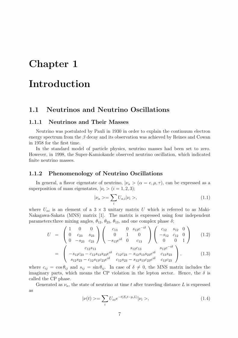
In general, a flavor eigenstate of neutrino, |να > (α = e, µ, τ), can be expressed as asuperposition of mass eigenstates, |νi > (i = 1, 2, 3);
|να >=∑
i
Uα,i|νi >, (1.1)
where Uαi is an element of a 3 × 3 unitary matrix U which is referred to as Maki-Nakagawa-Sakata (MNS) matrix [1]. The matrix is expressed using four independentparameters:three mixing angles, θ12, θ23, θ13, and one complex phase δ;
U =
1 0 00 c23 s23
0 −s23 c23
c13 0 s13e−iδ
0 1 0−s13e
iδ 0 c13
c12 s12 0−s12 c12 0
0 0 1
(1.2)
=
c12s13 s12c13 s13e−iδ
−s12c23 − c12s13s23eiδ c12c23 − s12s13s23e
iδ c13s23
s12s23 − c12s13c23eiδ c12s23 − s12s13c23e
iδ c13c23
, (1.3)
where cij = cos θij and sij = sin θij. In case of δ 6= 0, the MNS matrix includes theimaginary parts, which means the CP violation in the lepton sector. Hence, the δ iscalled the CP phase.
Generated as να, the state of neutrino at time t after traveling distance L is expressedas
|ν(t) >=∑
i
Uαie−t(Eit−piL)|νi >, (1.4)
7

CHAPTER 1. INTRODUCTION
where Ei and pi are the energy and momentum of νi in the laboratory frame, respectively.In practice, neutrino is extremely relativistic due to the tinniness of the mass, and thuswe can make following approximations:
t ∼ L, (1.5)
Ei =√
p2i + m2
i ∼ pi +m2
i
2pi
(1.6)
Since να is produced with a definite momentum p all of να’s mass eigenstates have acommon momentum. Thus, the probability P (να → νβ) that νβ is observed after να
travels the distance the distance L is given by
P (να → νβ) = | < νβ|ν(t) > |2 = |∑
i
UαiU∗βie
−ipLe−im2
i L
2p |2 (1.7)
= δαβ − 4∑i>j
Re(UαiU∗βiU
∗αjUβj) sin2
[1.27∆m2
ij
L
E
]−4∑i>j
Im(UαiU∗βiU
∗αjUβj) sin2
[2.54∆m2
ij
L
E
]where ∆m2
ij ≡ m2i − m2
j is the mass squared difference between νi and νj in eV2, L is inkm, and E is in GeV. The sign of the last term in Eq. 1.7 is + instead of − in the case ofthe expression for antineutrino. Because of the condition ∆m2
12 + ∆m223 + ∆m2
31 = 0 tobe imposed, the number of independent parameters for neutrino oscillations is six in thecase of three lepton generations: three mixing angles, (θ12, θ23, θ31), one CP phase, δ, andany two out of three mass squared difference, ∆m2’s.
1.1.3 Summary of Neutrino Oscillation Measurements
There are many neutrino oscillation measurements such as atmospheric neutrino ob-servations, solar neutrino observations, reactor neutrino experiments and accelerator neu-trino experiments. Figure 1.1 shows allowed or excluded regions from various experiments.In summary, there are two allowed regions:
1. Atmospheric region: ∆m223 ∼ 2.5 × 10⁻³ eV2, θ23 ∼ 45 degrees
The neutrino oscillation in the atmospheric region was discovered with the νµ → νx
oscillation by the Super-Kamiokande (SK) group [2]. This is the first discovery ofthe neutrino oscillation. The result have been confirmed by two long base-lineaccelerator neutrino experiments (K2K [3] and MINOS [4]).
2. Solar region: ∆m212 ∼ 8 × 10⁻⁵ eV2, θ12 ∼ 30 degrees
The neutrino oscillation in the solar region was discovered with νe → νx oscillationby solar neutrino experiments ( [5],SNO [6] and SK [7]) and confirmed by a reactorneutrino experiment;KamLAND [8].
Meanwhile, the θ13 and δ have never been measured to be nonzero. Some reactor experi-ments [9,10] searches θ13 with the νe → νx oscillation and gives the 90% C.L. (ConfidenceLevel) upper limit as
sin2 2θ13 < 0.15, (1.8)
8

CHAPTER 1. INTRODUCTION
Cl 95%
Ga 95%
νµ↔ν
τ
νe↔ν
X
100
10–3
∆m
2 [
eV
2]
10–12
10–9
10–6
102 100 10–2 10–4
tan2θ
CHOOZ
Bugey
CHORUS NOMAD
CHORUS
KA
RM
EN
2
PaloVerde
νe↔ν
τ
NOMAD
νe↔ν
µ
CDHSW
NOMAD
K2K
KamLAND
95%
SNO
95%Super-K
95%
all solar 95%
http://hitoshi.berkeley.edu/neutrino
SuperK 90/99%
All limits are at 90%CL
unless otherwise noted
LSND 90/99%
MiniBooNE
MINOS
Figure 1.1: Allowed or excluded regions in the tan2 θ-∆m2 plane from various experi-ment; There are two allowed regions around ∆m2 ∼ 10−3 (tan2 θ ∼ 1) and ∆m2 ∼ 10−5
(tan2 θ ∼ 1/3) which are corresponding to the atmospheric and solar regions, respectively.In addition, there is one allowed region around ∆m2 ∼ 1. However, most of the region isexcluded by other experiments such as MiniBooNE.
when ∆m223 ∼ 2.4 × 10⁻³ eV2 [11]. The θ13 can be also constrained by searching the
νµ → νe oscillation in long base-line accelerator neutrinos. This channel has beenstudied by K2K [12] and MINOS [13]. The signal of νµ → νe oscillation has not beenobserved so far.
1.1.4 Next Step of Neutrino Oscillation Experiment
As shown above, θ12 and θ23 are measured to be nonzero value and confirmed byseveral experiments with different methods. However, θ13 has never been measured to benonzero value and just upper limit is known so far. As shown in Eq. 1.2, the CP phaseδ enters only the MNS matrix in combination with sin θ13. Hence, δ never appear on theexpressions of the transition probabilities for any possible neutrino oscillations if θ13 iszero. In case of non-zero θ13, the CP phase can be extracted by calculating the asymmetryof the transition probability for the νµ → νe and νµ → νe oscillations as
A =P (νµ → νe) − P (νµ → νe)
P (νµ → νe) + P (νµ → νe)=
∆m212L
4Eν
· sin 2θ12
sin θ13
· sin δ. (1.9)
9

CHAPTER 1. INTRODUCTION
Therefore, measuring θ13 is one of the main motivations for the neutrino oscillation ex-periments.
Since the probability of the νµ → νe transition is small, the most plausible scenarioof the νµ → νx oscillation is that muon neutrinos oscillate to tau neutrinos (νµ → ντ ).However, the νµ → ντ transition is not observed yet. The detection of ντ s is difficultbecause their energy threshold for charged current τ production (3.4 GeV) is higher thanthe neutrino energy maximizing the νµ → νx oscillation in K2K, T2K and MINOS. Theidentification of ντ is also difficult because τs decay to multiple particles in many wayswithin short life time (∼0.3 ps). No observation of the νµ → ντ transition makes it possiblealternative scenario of the νµ → νx oscillation that muon neutrinos oscillate with sterileneutrinos (νs). The sterile neutrinos do not have neither charged current nor neutralcurrent interactions. Since the number of the light neutrino flavors interacting via weakcurrent is measured to be three with the decay width of Z0, any additional light neutrinomust be sterile neutrino. The search for sterile neutrino is also the motivations for theneutrino oscillation experiments.
1.2 Neutrino-nucleus Interaction
The long baseline (LBL) neutrino oscillation experiments play important roles in fur-ther understandings of the neutrino oscillation. To measure θ13 by searching νµ → νe
oscillation, the T2K experiment recently started [14] and the NOνA [15] experiment isnow under construction aiming at the first run in 2014. The MINOS experiment [11]is currently running mainly for the precise measurements of νµ → νx and νµ → νx
oscillations. In addition, such LBL experiments can perform sterile neutrino search.For the best performance of the LBL experiments, understandings of neutrino-nucleus
interaction in the few-GeV neutrino energy range are important. In such neutrino energyrange, a neutrino interacts with nucleons in the nucleus (or entire nucleus) in the followingprocesses via charged current (CC) and neutral current (NC):
• quasi-elastic scattering (νN → `N ′)
• single pion production (νN → `N ′π, or νA → `Aπ)
• deep inelastic scattering (νN → `N ′ + hadrons)
where N and N ′ are the nucleons (proton or neutron), A is the nucleus, ` is the lepton.In general, there are only a handful of cross section measurements in the few-GeV
neutrino energy range, and their precision is limited by small statistics. Therefore, theprecise measurements of neutrino-nucleus interactions are desired. Among the severalinteraction processes, the π0 production via neutral current (NCπ0, νµ+N → νµ+π0+N ′)is the one of the most important processes for the νµ → νe oscillation search.
1.3 Neutral Current π0 Production
In this section, we describe the importance of NCπ0, the π0 production mechanismsand the measurement of NCπ0.
10

CHAPTER 1. INTRODUCTION
1.3.1 Importance of NCπ0 Production
The NCπ0 production is the key of the next step of the neutrino oscillation experimentsdescribed in Section 1.1.4. We describe the importance of NCπ0 production in detailbelow.
Background for the νµ → νe Search
Here, we focus on the search for νµ → νe oscillation in the T2K (Tokai-to-Kamioka)experiment. The T2K experiment is a new long-baseline neutrino experiment using theSuper-Kamiokande (SK) as the far detector. In T2K, the charged current quasi-elastic(CCQE, νe + n → e + p) interaction is used to identify the νe signal at SK. Since SK isa ring-imaging water Cherenkov detector, the electron from νe is detected as a electron-like (e-like) cherenkov ring. Typically the momentum of a recoil proton in the CCQEinteraction is below the Cherenkov threshold in the water. Therefore only the electron,visible as a single-ring e-like event, is the signature of νe appearance. The probability of
Figure 1.2: The νe spectrum at SK with (sin2 2θ13, ∆m2) = (0.1, 2.5×10⁻³eV2). The sumof νe signals and backgrounds is shown by the dots with error bars, and two histogramsshow the total background and the νµ background, respectively.
the νµ → νe oscillation is proportional to sin2 2θ13, which is small (Eq. 1.8). Therefore,precise understanding of the background is crucial. Figure 1.2 shows the expected νe
energy spectrum at SK with (sin2 2θ13, ∆m2) = (0.1, 2.5×10⁻³eV2) with the backgroundcontamination. In the figure, the sum of νe signals and backgrounds is shown by the dotswith error bars, and two histograms show the total background and the νµ background,respectively. As shown in the figure, the νµ background is the one of main backgrounds.The main contribution of the νµ background is the neutral current π0 (NCπ0) productionby νµ. In SK, a single π0 decaying into two gamma rays can be classified as a single-ring, e-like event (νe candidate), when one gamma ray is not reconstructed due to highly
11

CHAPTER 1. INTRODUCTION
asymmetric energies or a small opening angle between the two gamma rays. Non νµ
background is coming from the intrinsic νes, which are produced in the neutrino beamproduction not by the νµ → νe oscillation.
Figure 1.3 shows the T2K’s sensitivity to sin2 2θ13 as a function of the beam exposurewhose unit is 22.5 kt (SK′s fiducial volume) × one year. The intensity of the primaryproton beam is assumed to be 750 kW. The three lines show three different levels ofuncertainties in the subtraction of the NCπ0 and beam intrinsic νe. For these exposures,the difference between 10 % and 0% uncertainties is minor, but between 10 % and 20 %there is a noticeable change. For this reason a 10 % uncertainty on the NCπ0 cross sectionis desired. As described in Section 1.3.2, there are no measurements of NCπ0 cross sectionwith less than 10 % uncertainty at the neutrino energy of T2K (∼ 0.8 GeV) ∗
Sensitivity 750kW13θ90% CL
Exposure/(22.5kt x 1year)-110 1
sen
sitiv
ity13θ
2
2si
n
-310
-210
-110
Systematic Error Fraction
5% sys error
10% sys error
20% sys error
Normal Hierarchy
Sensitivity 750kW13θ90% CL
Figure 1.3: The expected 90 % Confidence Level (CL) sensitivities for measuring sin2 2θ13
for uncertainties 0 % (bottom curve), 10 % (middle curve) and 20 % (top curve) inbackground subtraction.
Signal for the Sterile Neutrino Search
A single π0 event is a good signature of NC interactions in the GeV region especially fora water cherenkov detector such as SK because a π0 decay is clearly identified as two e-likeCherenkov rings. The single π0 production rate by the T2K neutrino beam or atmosphericneutrinos could be usable to distinguish between the νµ → ντ and νµ → νs oscillationhypotheses. Since the sterile neutrinos (νs) have neither CC nor NC interaction, the NCrate is attenuated in the case of transitions of νµ’s into sterile neutrinos. Meanwhile,the NC rate does not change in the νµ → ντ scenario, and the NC measurements candistinguish the two hypotheses.
∗After our result of the NCπ0 cross section measurement was submitted to Physical Review D (PRD),the MiniBooNE collaboration also submitted the result of the NCπ0 cross section measurement to PRD[16]. Our measurement and MiniBooNE use the common neutrino beam whose energy is ∼ 0.7 GeV andthe uncertainties of their measurement are less than 10 %. Hence, there exist two NCπ0 measurementswithin a 10 % uncertainty at the similar neutrino energy to T2K.
12

CHAPTER 1. INTRODUCTION
1.3.2 π0 Production Mechanisms and Measurements
In the neutrino energy rage of a few GeV, pion production through a neutrino scat-tering on nuclei principally occurs by two mechanisms; the resonant pion production andthe coherent pion production.
Resonant Pion Production
The larger contribution of the π0 production comes from incoherent processes in whichthe neutrino interacts with one of the nucleons in the nucleus. In the energy range of a fewGeV, the incoherent process mainly consists of the excitation and subsequent pionic decayof baryonic resonances such as ∆ (1232). Both CC and NC resonant pion productions arepossible. Considering π0 production via neutral current interaction by neutrinos, thereare two channels:
νµp → νµpπ0 (1.10)
νµn → νµnπ0 . (1.11)
There exist several theoretical models. Fogli and Narduli [17] expressed the nucleon-resonance transition amplitude with the vector form factors and axial form factors as-suming usual hypotheses such as CVC (conserved vector current) and PCAC (partiallyconserved axial vector current). Then, Fogli and Narduli calculated the cross section of thesingle pion production considering the resonances with mNπ < 1.6 GeV and non-resonantcomponent. The Rein and Sehgal [18] summed all resonances up to mNπ < 2.0 GeV,using quark model predictions. Since the Rein and Sehgal model is used in our analysesas well as widely used in neutrino oscillation experiments, we will describe the details inSection 4.2.1. Table 1.1 shows the comparison of the cross section of NC resonant π0 pro-duction between the Rein and Sehgal model and the Fogli and Narduli model. The 10-20% difference between them is seen. We note that these models predict the single pioncross section only via the neutrino-nucleon interaction. However, the neutrino targetsused for recent experiments are generally not hydrogen but heavier nucleus such as car-bon, water, iron and so on. In these cases, the resonance production and its decay couldbe different from a simple picture of neutrino-nucleon interactions due to nuclear effectssuch as Fermi motion, Pauli blocking and nuclear potential. Therefore, we need to takethe nuclear effects into account. For our analyses, such nuclear effects are implementedwith Rein-Sehgal model as described in Chapter 4.
Table 1.1: Comparison of the flux averaged calculated cross-section for the beams ofANL(0.4-6.0 GeV, [19, 20]) and Gargamelle(1-10 GeV, [21]) with the Rein and Sehgal(RS) model and the Fogli and Narduli (FN) model (in the unit of 10−38cm2).
mode ANL(0.4-6.0 GeV) Gargamelle(1-10 GeV)RS FN RS FN
σ(νpπ0) 0.035 0.036 0.083 0.090σ(νnπ0) 0.033 0.038 0.086 0.105
13

CHAPTER 1. INTRODUCTION
There exist several other model calculation for the single resonant pion productionincluding nuclear effects by Athar [22], Praet [23] and Martini [24]. In Athar’s model,the ∆ production cross section via simple neutrino-nucleon interaction is modified byusing local density approximation where neutrino interacts with a nucleon moving insidethe nucleus of density ρ(r) with its corresponding momentum ~p constrained to be below
its Fermi momentum pF (r) = [3π2ρ(r)]13 . In Praet’s model, they include nuclear effect
adopting impulse approximation: the nuclear many-body current is replaced by a sumof one-body current operators, and assuming an independent-particle model where theinitial-nucleon free Dirac spinor is replaced by a bound-state spinor. Both in Athar’sand Praet’s model, the width and mass of the ∆ is modified so that the ∆ properties innuclear medium are included. In the Martini’s model, they introduce the nuclear responsefunctions and related them to the hadronic tensor W µν which is contracted with the leptontensor as W µνLµν to obtain the amplitude. In these three models, only ∆ resonance istaken into account so that the cross section may be underestimated. Figure 1.4 shows thecomparison of several theoretical predictions for the charged current single π+ productionwithout final state interaction (FSI, which we will describe later). There are significantdiscrepancies among the predictions The experimental input on the NCπ0 cross section isneeded to choose or correct theoretical models.
Figure 1.4: The comparison of several theoretical predictions of the total incoherent CCπ+ production on Carbon without the final state interaction. Genie [25], Neut (Chap-ter 4.2) and NuWro [26] are the Monte Carlo generators with the Rein and Sehgal model.(The plots is from the presentation by J.Sobczyk for “Sixth International Workshop onNeutrino-Nucleus Interactions in the Few-GeV Region”)
There is another nuclear effect called final state interaction where nucleons and mesonsproduced in the primary neutrino-nucleon interaction interact with nuclear matter beforeexiting the nucleus. The final state interactions of nucleons and mesons in the targetnucleus could largely modify the number, momenta, directions and charge states of pro-duced particles. Though there exist several theoretical approaches for modeling theseprocesses, their uncertainties are large. Therefore, the kinematics of π0s after exitingnucleus are important to compare the theoretical predictions with the experimental ob-servation Therefore, measurements of not only the overall cross section but also emittedπ0 kinematics of NCπ0 production are important.
14

CHAPTER 1. INTRODUCTION
Table 1.2: Past measurements of neutral current resonant π0 production by neutrinos.
Experiment Eν (GeV) Target Result
Gargamelle 1978 1-10 Propaneσ(νµpπ0)+σ(νµnπ0)
2σ(µ−pπ0)= 0.45 ± 0.08
BNL 1976 0.5-14.5 Al, Cσ(νµNπ0)
σ(µ−N ′π0)= 0.17 ± 0.04,
σ(νµNπ0)
σ(µ+N ′π0)= 0.39 ± 0.18
ANL 1981 0.4-6.0 H2, D2
σ(νµpπ0)σ(µ−pπ+)
= 0.09 ± 0.05
K2K 2005 ∼1.3 H2Oσ(νµNπ0)
σ(CC) = 0.064 ± 0.001stat. ± 0.007sys.
For resonant π0 production via neutral current interactions, several experimental mea-surements using GeV neutrino have been performed in the past 40 years as shown inTable 1.2. Measurements in early dates were performed in bubble chamber experiments:ANL [19, 20]. Gargamelle [21], and spark chamber experiments in BNL [27]. The pre-cision of the measurements is at a 20% level, limited by low statistics. In addition, theresults are expressed as the ratio to the charged current (CC) single pion production crosssection, which is also poorly known. This is not a useful expression for predicting electronbackgrounds in νµ → νe oscillation searches, since the νµ flux is usually measured byinclusive CC or CCQE interaction in the long baseline neutrino oscillation experimentssuch as T2K.
Recently, two experiments published single π0 production results. Although theseexperiments measure inclusive (resonant + coherent) pion production, the most of contri-bution is resonant pion production ( the coherent fraction is less than 20 % ). The K2Kcollaboration reported the cross section ratio of the NC π0 production to total CC eventsin water with a 1.3 GeV mean neutrino energy beam [28]. Their result of the cross sectionratio is consistent with the Monte Carlo (MC) prediction based on the Rein and Sehgalmodel [18]. MiniBooNE reported the yield and spectral shape of π0 s as a function of π0
momentum in mineral oil (CH2) in neutrino beam of mean neutrino energy 0.7 GeV [29].However, they do not report the cross section or cross section ratio. The total NCπ0
cross section below 1 GeV has still not been precisely measured yet. This is the mainmotivation of our measurement.
Coherent Pion Production
A smaller contribution comes from coherent scattering where the neutrino interactswith the entire nucleus leaving it in the ground state. This means the effective dimensionsof space involved in the interactions is large compared with the dimensions of the targetnucleus, i.e.,
1
|t|> R, (1.12)
15

CHAPTER 1. INTRODUCTION
where t and R are the four-momentum transfer to the target nucleus and the radius ofthe target nucleus, respectively. Because of the small momentum transfer to the targetnucleus the outgoing lepton and pion tend to go in the forward direction in the lab frame,and no nuclear breakup occurs. Both charged current (CC) and neutral current (NC)coherent pion productions are possible;
νµA → µ−Aπ+ (1.13)
νµA → νµAπ0 , (1.14)
where A is a nucleus.There exist several theoretical models for coherent pion production. They are cate-
gorized into two different types. The first one is built on the basis of Adler’s PartiallyConserved Axial-vector Current (PCAC) theorem [30], associating the neutrino-nucleuscross section to the pion-nucleus cross section at Q2 = 0, where Q2 ≡ −(P` − Pν)
2 isthe square of the four-momentum transfer, and P` and Pν are the four-momenta of theoutgoing lepton and the incoming neutrino, respectively; the extrapolation to Q2 6= 0 isdone via a propagator term [31–35]. The second one is based on the description of thecoherent production of ∆ resonances on nuclei by using a modified ∆-propagator and adistorted wave-function for the pion [36–38].
The model of Rein and Sehgal [32, 35], one of the first category, is commonly used inneutrino oscillation experiments. Since the Rein-Sehgal model is used for this thesis, thedetails are described in Section 4.2.1. Figure 1.5 shows the predicted or calculated crosssections for νµ
12C→ µ−π+12C interaction. The solid line and the dashed line represent theRein and Sehgal model with lepton mass effects [35] and without lepton mass effects [32],respectively. The cross sections predicted by other recent models are also shown in thefigure. As shown in the figure, order-of-magnitude variation on the coherent pion produc-tion cross section exist among the different models. Therefore, more experimental inputon coherent pion production in neutrino-nucleus interactions is needed.
Table 1.3: List of past measurements of coherent pion production. The experimentalresults are summarized in Figure 1.6
Experiment Beam Reaction Eν (GeV) Target 〈A〉 ReferenceAachen-Padova (AP) νµ/νµ NC 2 Al 27 [39]Gargamelle (GGM) νµ/νµ NC 3.5 Freon 30 [40]SKAT νµ/νµ CC/NC 3-30 Freon 30 [41]CHARM νµ/νµ NC 10-160 Marble 20 [42]CHARM II νµ/νµ CC 3-300 Glass 20.1 [43]BEBC (WA59) νµ/νµ CC 5-150 Ne 20 [44,45]FNAL E632 νµ/νµ CC 10-300 Ne 20 [46,47]K2K νµ CC 1.3 C 12 [48]MiniBooNE νµ NC 1.2 C 12 [29]
Coherent pion production has already been the subject of several experimental cam-paigns. Table 1.3 summarizes the past measurements of coherent pion production. Al-though there exist positive coherent pion production results at higher energy (3-300 GeV
16

CHAPTER 1. INTRODUCTION
(GeV)νE0 0.5 1 1.5 2 2.5 3
/Car
bo
n n
ucl
eus)
2cm
-40
(10
CC
σ
0
10
20
30
40
50
60
70
80
90
100
Figure 1.5: Cross section for νµ12C→ µ−π+12C interaction. The solid line represents the
Rein and Sehgal model with lepton mass effects [35], the dashed line represents the Reinand Sehgal model without lepton mass effects [32], the dotted line represents the modelof Kartavtsev et al. [34], and the dashed-dotted line represents the model of Alvarez-Rusoet al. [38]. The model of Singh et al. [36] gives a cross section similar to the model ofAlvarez-Ruso et al.
0
0.2
0.4
0.6
0.8
1
1.2
1.4
0 5 10 15 20Eν (GeV)
σ(ν µ
C →
µ- C
π+ )
(10-3
8 cm
2 )
MB
K2K
AP
GGM
SKAT
CHARM,BEBC
ν CCanti-ν CCν NCanti-ν NC
Figure 1.6: Existing experimental results on the coherent pion production cross section(Eν < 20 GeV). The results are scaled to the cross section for νµ
12C→ µ−π+12C byassuming (a) σ(CC) = 2σ(NC), (b) σ(νµ) = σ(νµ), and (c) A2/3 dependence. For theK2K result, the upper limit on the cross section ratio to total charged current is convertedusing the predicted value of the total charged current cross section quoted in their paper.Similarly, for the MiniBooNE result, the cross section ratio to all neutral current singleneutral pion production is converted using the Rein-Sehgal prediction for resonant pionproduction.
17

CHAPTER 1. INTRODUCTION
neutrino energy) via charged and neutral current interactions, the K2K experiment witha 1.3 GeV wide-band neutrino beam [48] reports null observation of charged currentcoherent pion production. This result is confirmed by the SciBooNE experiment [49].Meanwhile, the MiniBooNE Collaboration with similar neutrino energy to K2K observesthe neutral current coherent pion production but their observation is 65 % of the Reinand Sehgal prediction. We also show a summary of existing experimental results on thecoherent pion production cross section below 20 GeV in Figure 1.6. The Rein and Sehgalmodel well explains these experimental measurements except for results from the K2K,SciBooNE and MiniBooNE experiments. From these facts, the coherent pion productionhave drawn much attention in the neutrino interaction physics community in addition tothe importance for the νµ → νe oscillation search. Hence, it is interesting to confirm theNC coherent π0 production.
1.4 Overview of This Thesis
In this thesis, we present measurements of the NCπ0 interaction in polystyrene (C8H8)with mean neutrino energy 0.7 GeV. We measure the ratio of the total inclusive NCπ0
cross section to the total CC cross section and kinematic distributions of the π0s. Wealso extract the fraction of coherent NC π0 events in the inclusive NC π0 data sample. Inthese analyses, we define NCπ0 events to be NC neutrino interactions with at least oneπ0 emitted in the final state from the target nucleus.
The measurement in this thesis is the first high statistic NCπ0 measurement at themean neutrino energy below 1 GeV. Hence, it helps the νµ → νe oscillation search, espe-cially for T2K. Our measurements use the fully active scintillating tracker as describedin Chapter 3 while the existing high statistic π0 production measurements are usingCherenkov detectors. Hence, our measurements provide new approach to the π0 produc-tion via neutrino interactions, which is important information for the future developmentsof π0 detection and reconstruction techniques. In addition, we could observe the recoilprotons via neutrino interactions due to the full activity of the scintillating tracker. Usingthe information of the recoil proton, we can unambiguously distinguish the coherent pionproduction from the incoherent pion production since the proton recoil occurs only in theincoherent pion production. For these reasons, the measurements presented in this thesisis very much important for the neutrino physics.
This thesis is organized as follows. Chapter 2 describes the overview of the SciBooNEexperiment. In Chapter 3, we describe the experimental setup including the neutrinobeamline, the detector configuration, and the data set. In Chapter 4, we describe theMonte Carlo (MC) simulations for the neutrino flux prediction, neutrino interactionswith nuclei and the particle transportation in the detector. In Chapter 5, we describethe event selection for the NC π0 events. Then, in Chapter 6, we discuss the study ofthe NCπ0 production including the measurement of the ratio of the NCπ0 production tototal charged current cross sections, the π0 kinematic distribution and the coherent pionextraction. The conclusions are given in Chapter 7.
18

Chapter 2
SciBooNE Experiment
In this chapter, we describe the overview and physics motivations of the SciBooNEexperiment.
2.1 Overview of SciBooNE
The SciBar Booster Neutrino Experiment (SciBooNE) [50] is designed for measuringthe neutrino-nucleus cross sections around one GeV region, which is essential for neutrinooscillation experiments such as T2K. We briefly summarize features of the SciBooNEexperiment;
• High intensity low energy neutrino beamSciBooNE uses the Booster Neutrino Beam (BNB) at Fermi National AcceleratorLaboratory (FNAL), which has been used for the MiniBooNE experiment. The BNBcan provide a high rate and low energy neutrino beam. In the BNB, an antineutrinobeam can be produced by reversing the polarity of the horn current.
• Fully active fine segmented scintillator tracking detectorSciBooNE uses the Scintillator Bar (SciBar) detector, a fully active fine segmentedtracking detector. The SciBar detector was originally developed and used for theK2K experiment [51]. SciBar acts as the neutrino target, and also can detect allcharged particles produced by neutrino interactions.
These two main feature give us an efficient opportunity for precise measurements of neu-trino cross sections since both are already built and have been operated successfully.
Figure 2.1 shows a schematic drawing of the experimental setup of SciBooNE. TheSciBooNE detector is positioned 100 m downstream from the proton target on the axisof the beam. The MiniBooNE detector is located 440 m downstream from the SciBooNEdetector, exposed by the same neutrino beam. The detector comprises three sub-detectors;the SciBar detector is followed by an electromagnetic calorimeter (EC) and a muon rangedetector (MRD). Detailed descriptions of the BNB and the SciBooNE detector are givenin Chapter 3.
19

CHAPTER 2. SCIBOONE EXPERIMENT
50 m
100 m 440 m
MiniBooNE
Detector
Decay region
SciBooNE
DetectorTarget/Horn
Figure 2.1: Schematic drawing of the experimental setup of SciBooNE.
2.2 Physics Motivations of SciBooNE
SciBooNE has three main physics motivations: precise measurements of neutrino-nucleus cross sections, measurements of antineutrino-nucleus cross sections, and the BNBneutrino flux measurements.
2.2.1 Precise Measurements of Neutrino-nucleus Cross Sections
Figure 2.2 shows the νµ energy spectrum at SciBooNE with those at K2K and T2K.Since the entire range of the T2K energy spectrum is covered within the spectrum ofSciBooNE, various neutrino cross section measurements at SciBooNE could help neutrinooscillation studies in T2K. The measurement of the NCπ0 production is classified intothis category and the primary motivation of the SciBooNE experiment.
0
0.5
1
0 1 2 3Eν (GeV)
Flu
x (A
rbitr
ary
unit)
K2K
T2K
SciBooNEFigure 2.2: Comparison of the muon neu-trino energy spectra at K2K, T2K, andSciBooNE. All curves are normalized tounit area.
2.2.2 Measurements of Antineutrino-nucleus Cross Sections
If a non-zero θ13 is found, T2K will search for CP violation in the neutrino sector. Itrequires oscillation measurements with both neutrino and antineutrino beams. However,the current knowledge of antineutrino cross sections in the few GeV range is very poor
20

CHAPTER 2. SCIBOONE EXPERIMENT
with few low statistics measurements. SciBooNE can measure various antineutrino crosssections with high precision.
2.2.3 BNB Neutrino Flux Measurements
The νµ flux normalization and energy spectrum measured by SciBooNE can be use forneutrino oscillation searches at MiniBooNE. The sensitivity study of νµ → νx and νµ → νx
oscillations with flux normalization and shape systematics [50] indicates the utility of anexternal measurement of the neutrino flux. In the νµ → νx oscillation search, it is crucialto understand the wrong-sign (νµ) background, and we can extract the normalization andenergy spectrum of the background by using the SciBooNE experiment.
21

Chapter 3
Experimental Setup and Data Set
In this chapter, we describe the experimental setup of the SciBooNE experiment. Wealso describe the data set used for this analysis.
3.1 Booster Neutrino Beam
Fermilab Booster accelerates the protons up to 8 GeV kinetic energy. Selected spillscontaining approximately 4-5×10¹² protons are extracted and bent toward the BNB targethall. Each spill contains 81 bunches of protons, approximately 6 nsec wide each and19 nsec apart, for a total spill duration of 1.6 µsec. The typical beam alignment anddivergence, measured by the beam position monitors located near the target, are within 1mm and 1 mrad of the nominal target center and axis direction, respectively. The typicalbeam focusing on target measured by the beam profile monitors is of the order of 1-2 mm(RMS) in both the horizontal and vertical directions. The number of protons delivered tothe BNB target for each spill is measured with a 2% accuracy using two toroidal currenttransformers (often referred to as toroid’s) located near the target along the beamline.These parameters are well tuned within the experiment requirements.
3.1.1 Target and Magnetic Focusing Horn
The primary proton beam smashes a thick beryllium target located in the BNB targethall. Secondary mesons (pions and kaons) are produced by hadronic interactions of theprotons with the target. The target is made of seven cylindrical slugs with a radius of0.51 cm, for a total target length of 71.1 cm, or about 1.7 inelastic interaction lengths.The target is surrounded by a magnetic focusing horn, focusing the positively-charged sec-ondary particles from the target to the direction pointing to the SciBooNE detector. Suchpositively-charged secondary particles are dominated by charged pions (pi+) producingthe neutrino beam via their decay (pi+ → µ+νµ) The focusing is produced by the toroidalmagnetic field present in the air volume between the horn’s two coaxial conductors madeof aluminum alloy. The horn current pulse is approximately a half-sinusoid of amplitude174 kA, 143 µsec long, synchronized to each beam spill. The polarity of the horn currentflow can be (and has been) switched, in order to focus negatively-charged mesons, andtherefore to produce an antineutrino beam instead of a neutrino beam.
22

CHAPTER 3. EXPERIMENTAL SETUP AND DATA SET
3.1.2 Decay Region and Absorber
The secondary mesons from the target/horn region are further collimated via passiveshielding, and moved to a cylindrical decay region where the secondary mosons can decayinto neutrinos. The decay region is filled with air at atmospheric pressure, 50 m long and90 cm in radius. A beam absorber located at the end of the decay region stops hadronicparticles and muons, and only a pure neutrino beam pointing toward the detector remains,mostly from π+ → µ+νµ decays.
3.2 SciBooNE Detector
A schematic drawing of the SciBooNE detector is shown in Figure 3.1. The SciBooNEdetector consists of three sub-detectors: a fully active and finely segmented scintillator bartracker (SciBar), an electromagnetic calorimeter (EC) and a muon range detector (MRD).In the following sections, sub-detectors and the data acquisition system are described. Thedetector coordinate are also described.
ν-beam
SciBarEC
Dark box
4m
2m
MRD
Figure 3.1: Schematic drawing of the SciBooNE detector.
23

CHAPTER 3. EXPERIMENTAL SETUP AND DATA SET
3.2.1 Scintillator Bar Tracker (SciBar)
The SciBar detector is located at the upstream of the other sub-detectors. The mostimportant role of SciBar is to reconstruct the neutrino-nucleus interaction vertex and de-tect charged particles produced by neutrino interactions. In addition, SciBar can identifyparticles based on energy deposition per unit length. SciBar was originally designed andbuilt as a near detector for the K2K experiment [51]. After K2K was completed, theSciBar detector was once disassembled, shipped to FNAL, and then re-built there forSciBooNE.
Figure 3.2 shows a schematic drawing of SciBar. The SciBar detector consists of 14,336extruded plastic scintillator strips which serve as the target for the neutrino beam as wellas the active detection medium. Each strip has dimensions of 1.3 × 2.5 × 300 cm3. Thescintillators are arranged vertically and horizontally to construct a 3× 3× 1.7 m3 volumewith a total mass of 15 tons. Each strip is read out by a wavelength shifting (WLS)fiber, Kuraray Y11(200)MS attached to a 64-channel multi-anode photomultiplier tube(MA-PMT), Hamamatsu H8804 as shown in Figure 3.3. The hit finding efficiencies eval-uated with cosmic ray data are 99.8 % and 99.9 % for the vertical and horizontal planes,respectively. The track finding efficiency for single tracks of 10 cm or longer is more than99 %. The radiation length of polystyrene (scintillator material) is approximately about43 cm. Since the length of SciBar along the beam axis is 1.7 m, SciBar has the thicknessof 4.0 radiation length. Table 3.1 summarizes specifications of the SciBar detector. In thefollowing sections, we describe the readout electronics, the gain monitoring system andthe energy calibration in details.
1.7m
EM calorim
eter
Extruded Scintillators (15ton)
64ch Multi−AnodePMT
Wave−lengthshifting fiber
3m
3m
Figure 3.2: Schematic drawing of SciBar.
24

CHAPTER 3. EXPERIMENTAL SETUP AND DATA SET
Table 3.1: Specifications of the SciBar detector
StructureDimensions 3 m × 3 m × 1.7 mWeight 15 tonsNumber of channels 14,336
ScintillatorMaterial Polystyrene, PPO(1%), POPOP(0.03%)Emission peak wavelength 420 nmReflector material TiO2(15%) infused in polystyreneDimensions 1.3 cm × 2.5 cm × 300 cmDensity 1.021 g/cm3
WLS fiberType Kuraray Y11(200)MS, multi-cladMaterial polystyrene(core), acrylic(inner), polyfluor(outer)Refractive index 1.56(core), 1.49(inner), 1.42(outer)Absorption peak wavelength 430 nmEmission peak wavelength 476 nmDiameter 1.5 mmAttenuation length 350 cm (typical)
MA-PMTModel Hamamatsu H8804Anode 8×8 pixels (pixel size: 2×2 mm2)Cathode Bialkali (Sb-K-Cs)Sensitive wavelength 300-650 nm (peak: 420 nm)Quantum efficiency 12% at λ=500 nmDynode Metal channel structure, 12 stagesGain typical 6 × 10⁵ at 800 VResponse linearity within 10% up to 200 photoelectrons
with the gain of 6 × 10⁵
Crosstalk 3.15% (adjacent pixel)Readout electronics
Number of ADC channels 14,336ADC pedestal width less than 0.3 photoelectronADC response linearity within 5% up to 300 photoelectrons
with the gain of 5 × 10⁵
Number of TDC channels 448TDC resolution 0.78 nsecTDC full range 50 µsec
25

CHAPTER 3. EXPERIMENTAL SETUP AND DATA SET
Figure 3.3: Schematic drawing of the SciBar readout system.
Readout Electronics
The readout electronics system consists of a front-end electronics board (FEB) at-tached to each MA-PMT and a back-end VME module [52]. Figure 3.4 shows the pictureof the FEB. On the FEB, a combination of VA and TA ASICs (IDEAS VA32HDR11 andTA32CG) is employed to multiplex pulse-height information from each anode of the MA-PMT and to make a fast-triggering signal. The VA has a 32-channel preamplifier-shapercircuit with a multiplexer. The slow shaper shapes the output with a peaking time of1.2 µsec. The signal from each VA slow shaper is sampled at the time of an external holdrequest, and the result is passed to the multiplexer. The signal after preamplification inthe VA is also sent to a fast shaper in the TA with a peaking time of 80 nsec. A logical“OR” of 32 channels is sent out from the TA. The intrinsic time jitter of the discriminatedoutput is less than 1 ns. The TA signal is sent to a 64-channel multi-hit time-to-digitalconverter (AMT [53]) and recorded as timing information. Each FEB has two packagesof VA/TA, processing 64-channel charge information and two-channel timing informationfor each MA-PMT. The back-end VME module, called the DAQ board, is developed asa standard VME-9U board. Figure 3.5 shows the picture of the DAQ board. Each DAQboard controls the readout of eight FEBs, and thus 28 DAQ boards are used in total.We use four VME-9U crates for all 28 DAQ boards (7 boards per 1 crate). Each of theeight channels in the single DAQ board has line drivers to control the VA and TA ASICson FEB and a 12-bit flash analog-to-digital converter (ADC) to digitize the multiplexedanalog signal from the FEB with a 1-MHz readout clock.
In the SciBooNE operation, the TA signal is used to generate the hold request forsampling the signal of each VA slow shaper. In fact, the DAQ board receives the TAsignal from the FEB and generate the hold request signal back to the FEB with 1.2 µsdelay. By doing this, the signal from the VA slow shaper is always sampled at its peakingtime. Therefore, the recorded charge information does not depend on when the neutrinointeractions happen during a total spill duration of 1.6 µsec. The timing sequence relatedto the TA, VA and hold request is shown in Figure 3.6.
The TA signal is also sent to a cosmic-ray trigger board. The board is a generalpurpose logic board powered by an FPGA, and programmed to generate a signal when
26

CHAPTER 3. EXPERIMENTAL SETUP AND DATA SET
a cosmic-ray penetrates almost all the layers of SciBar. The signal is used to record thecosmic-ray events which are useful to the calibration of SciBar and EC.
2 VA/TA chips(32 x 2 ch)
PMT signalline(AC coupling) for MAPMT
Mounting socket
+-5V -> +-2.4V
40pin flat connector
DAQ Board
Regulator
Figure 3.4: Picture of a front-end board.
(th
rou
gh
VM
Eb
us)
Gat
e, T
rig
ger
ID
16 (8x2) TAs(to TDC Module)
Figure 3.5: Picture of a DAQ board.
OutputPreanp.
Fast Shaper
Slow Shaper
TA
Hold
1.2 us
dizitized by ADC
80 ns
Figure 3.6: The timing sequence of the SciBar electronics
Gain Monitoring System
The gain stability of the MA-PMTs is ensured within ±2% by a custom-made mon-itoring system using light-emitting diodes (LEDs) [54]. The system consists of four setsof light sources, PIN photo-diodes, and clear fiber bundles. A schematic drawing of theSciBar gain monitoring system are shown in Figure 3.7. The pulsed light from each LEDis carried to 56 MA-PMTs through 56 clear fibers. A white cylinder, called a Light Injec-tion Module, is attached to the WLS fiber bundle in order to illuminate 64 WLS fibersuniformly. The LED light is absorbed by the WLS fibers, and then emitted light fromthe WLS fiber is carried to each channel of the MA-PMT.
27

CHAPTER 3. EXPERIMENTAL SETUP AND DATA SET
PINphoto
Light source Clear fiber
Light Injection Module
WLS fiber
Scintillator
MAPMT
Figure 3.7: Schematic drawing of the SciBar gain monitoring system.
Energy Scale Calibration
The energy scale for each channel is calibrated with cosmic-ray muons. The numberof photoelectrons for cosmic-ray muons for a typical channel are shown in Figure 3.8.The path length of the particle inside the scintillator strip and the light attenuation inthe WLS fiber are corrected. The averaged light yield of a minimum ionizing particle ismeasured to be approximately 20 p.e. per 1.3 cm path length. The energy calibrationconstant which converts the number of photoelectrons to the visible energy is measuredfor each channel. Figure 3.9 shows the energy calibration constants for all channels. Theaveraged value is 8.1 p.e./MeV, and the channel-by-channel variation is about 20%.
(p.e.)0 20 40 60 80 1000
2000
4000
6000
Figure 3.8: Number of photoelectrons forcosmic-ray muons for a typical channel.
Entries 14336
Mean 8.138
RMS 1.751
(p.e./MeV)0 5 10 15 20 250
500
1000 Entries 14336
Mean 8.138
RMS 1.751
Figure 3.9: Energy calibration constantsfor all channels.
3.2.2 Electromagnetic Calorimeter (EC)
EC is a “spaghetti” type electromagnetic calorimeter, installed downstream of SciBar,and is designed to measure the electron neutrino contamination in the beam and identify
28

CHAPTER 3. EXPERIMENTAL SETUP AND DATA SET
photons from π0 decay. The calorimeter modules were originally built for the CHORUSexperiment at CERN [55] and later used in HARP and then in K2K.
The calorimeter consists of modules of dimensions 262 × 8.4 × 4.2 cm3. The modulesconstruct one vertical and one horizontal plane, and each plane has 32 modules. An activearea of 2.7 × 2.6 m2 is covered by the planes. The EC has a thickness of 11 radiationlengths along the beam direction.
Each module is made of a stack of 21 lead sheets and 740 scintillating fibers. The 1 mmdiameter scintillating fibers, Kuraray SCSF81, are embedded in the grooves on 1.9 mmthick lead sheets. The stack is held together by a welded steel case. At each end of themodule, fibers are grouped into two bundles, and each bundle is connected to a Plexiglaslight guide. The light guide is attached to 1 inch PMT, Hamamatsu R1335/SM, with aspecial green-extended photocathode. A typical gain is 2 × 10⁶ at the operation voltageof 1600 V. In total, 256 PMTs are used in the EC. The attenuation length of the fiber ismeasured to be approximately 400 cm by using cosmic-ray muons. The readout systemconsists of eight 32-channel 12-bit QDC (Charge-to-Digital Converter) modules, CAENV792. One VME-6U crate is used for QDC readout. The energy resolution for electronswas measured to be 14%/
√E (GeV) in a test beam [55].
Figure 3.10: Schematic drawing of the EC module.
3.2.3 Muon Range Detector (MRD)
The MRD detector is installed downstream of the EC and is designed to measure themomentum of muons produced by charged-current neutrino interactions up to 1.2 GeV/cusing the range measurement. The MRD was constructed for SciBooNE at FNAL, pri-marily by using out of parts recycled from past FNAL experiments.
The MRD consists of 12 iron plates and 13 alternating horizontal and vertical scintil-lator planes. Each iron plate is 2 inch thick, and covers an area of 274 × 305 cm2. Thetotal mass of absorber material is approximately 48 tons. The iron plates are sandwichedbetween scintillator planes. Each scintillator plane consists of 20 cm wide, 6 mm thick
29

CHAPTER 3. EXPERIMENTAL SETUP AND DATA SET
scintillator paddles. Each vertical scintillator plane is comprised of 138 cm long paddles,arranged in a 2 × 15 array to have an active area of 276 × 300 cm2. On the other hand,each horizontal scintillator plane consists of 155 cm long paddles, arranged in a 13 × 2array to have an active area of 260×310 cm2. In total, 362 paddles are used in the MRD.
The scintillator paddles are read out by five types of 2 inch PMTs; the vertical planesconsist of Hamamatsu 2154-05 and RCA 6342A PMTs, the horizontal planes consist ofEMI 9954KB, EMI 9839b and 9939b PMTs. Charge and timing information from eachPMT are recorded. The readout electronics system consists of LeCroy 4300B ADCs andLeCroy 3377 TDCs. We use 13 TDCs and 26 ADCs housed in three CAMAC crates.The timing resolution and full range are 0.5 ns and 32 µsec, respectively. The energythreshold for TDC hits is approximately 250 keV which corresponds to 20% of the signalof a minimum ionizing particle. The single noise rate is typically 100 Hz except forRCA 6342A PMTs which are noisy (up to 104 Hz) Hit finding efficiency was continuouslymonitored by using cosmic ray data taken between beam spills. The average hit findingefficiency is measured to be 99%.
Table 3.2: Specifications of the MRD detector.
Iron plateNumber of plates 12Dimensions 274 × 305 cm2, 2 inch thicknessDensity 7.841 g/cm3
Scintillator planeNumber of planes 13Segmentation 2×15 (vertical), 13×2 (horizontal)Dimensions of a counter thickness: 6 mm, width: 20 cm
length: 138 cm (vertical), 155 cm (horizontal)PMT
Model Hamamatsu 2154-05, RCA 6342A (vertical)EMI 9954KB, 9839b and 9939b (horizontal)
Readout electronicsNumber of channels 362Model LeCroy 4300B (ADC), Lecroy 3377 (TDC)TDC resolution 0.5 nsecTDC full range 32 µsec
3.2.4 Trigger and Data Acquisition (DAQ) System
We describe the SciBooNE trigger and DAQ system in this section.
Beam Cycle
Each spill of the neutrino beam to SciBooNE is synchronized to the 15 Hz Boosterclock. However, not all counts of the Booster clock are occupied by the spills to SciBooNEas shown in Figure 3.11. In general, the neutrino beam comes to SciBooNE with several
30

CHAPTER 3. EXPERIMENTAL SETUP AND DATA SET
One beam cycle ~ 2 secondSciBooNEBeam to
Booster CLK15 Hz
Figure 3.11: SciBooNE’s beam cycle
continuous spills (up to 10 spills). Then, there is no beam period for more than 1.5 second.Since such several continuous spills and no beam period come to SciBar by turns, we callthis repetition “beam cycle”. We need to take calibration data during no beam period andstop taking calibration data before the spills come to SciBooNE. However, the number ofcontinuous spills and no beam period change depending on the operation modes of theaccelerator. Hence, the ways to generate beam triggers and calibration triggers are notstraightforward.
Table 3.3: Tevetron clocks (TCLKs) used for SciBooNE. The $10, $11, $12 and $1D aresynchronized to the $0C, which is 15 Hz Booster clock
TCLK code description$0C 15 Hz Booster clock$10 beam in Booster is accelerated and extracted somewhere$11 no beam in Booster$12 generated twice at the beginning of the beam cycle$1D beam in Booster is accelerated and extracted to SciBooNE$1F Booster kicker timing for extraction
To generate beam triggers and calibration triggers at the proper timing, we use severaltiming signals from the accelerator, called Tevetron clock (TCLK). TCLK is used totransmit important accelerator timing information to all major systems throughout theaccelerator complex. Up to 256 unique events or timing markers may be encoded ontoTCLK. Each TCLK is expressed by two digit hexadecimal number ($00-$FF). The TCLKsrelated to SciBooNE are $0C, $10, $11, $12, $1D and $1F. We show the descriptions aboutthese TCLKs in Table 3.3. Figure 3.12 shows the timing sequence of TCLKs and theSciBooNE triggers. The $0C is the 15 Hz Booster clock. The other TCLKs listed aboveare synchronized with $0C. At the beginning of the beam cycle, two $12s are generated.After the two $12s, several $10s are generated. The $10s let us know that the beamin Booster is accelerated and extracted. In case of the beam for the Booster neutrinobeamline, $1Ds are also generated with $10. After the train of the $10s, several $11s aregenerated. During $11s are generated, the beam is not in Booster. After the train $11s,the two $12s are generated again. This is how the beam cycle proceeds. Although thenumbers of $10s, $1Ds and $11 are not fixed permanently, typical period for one beam
31

CHAPTER 3. EXPERIMENTAL SETUP AND DATA SET
cycle is about 2 sec. We use the first one of two $12 to enable beam triggers and disablethe calibration triggers. By doing this, we disabled the calibration triggers by at least2 × 1/15Hz = 133 ms earlier than the next coming beam. This time is much longerthan the DAQ deadtime described later (20 ms). We use the first one of the $11’s trainto disable the beam triggers and enable calibration triggers. By doing this, we ensurethat the beam trigger is never missed due to the calibration trigger. We use the logicalAND of $1F and $1D for the beam triggers, where the $1F is the kicker timing for thebeam extraction. This is because the $1F has better timing resolution (100 ns) than$1D does. For practical purpose, one trigger is generated at the same time when thecalibration triggers are enabled by $11. We call such triggers off-beam triggers. Oneoff-beam trigger is generated per one beam cycle by definition. Since the beam triggerand off-beam trigger is commonly used by each component of the SciBooNE detectors,we call them global triggers.
&1F&1F
accelarator (TCLK)
SciBooNE
15 Hz Booster CLK"TCLK 0C"
Pre−Pulse "TCLK 1D"
&1F&1F
"TCLK 10"
Beam somewhere
No Beam "TCLK 11"
Beam to sciboone "TCLK 1D"
Beam Enable
Calibration Enable
Beam Triggers (Global)
Off−beam Triggers (Global)
LED
PedestalsCosmic rays
Calibration Triggers (Local)
Figure 3.12: The relation between TCLK and the SciBooNE trigger signals
The SciBooNE Trigger
The beam trigger (logical AND of $1D and $1F) is distributed to all three detectorsand used for the ADC gates and reference timings for TDCs. The beam trigger is alsodistributed to the PCI module called the Time and Frequency Processor, Symetricom
32

CHAPTER 3. EXPERIMENTAL SETUP AND DATA SET
bc637 PCI (GPS card). This GPS card is used for recording the GPS time for eachbeam trigger. Once the beam trigger condition is set, all sub-detector systems read outall channels irrespective of hit occupancy (i.e. whether or not a neutrino interactionoccurred), ensuring unbiased neutrino data.
SciBar and EC have common calibration triggers, which are the LED, pedestal andcosmic trigger. The LED trigger is for the gain monitor system of SciBar. Since nosuch gain monitor system in EC, the LED triggers are just pedestal triggers for EC.Meanwhile, MRD generates the pedestal and cosmic trigger independently from SciBar(EC). Therefore, the total numbers of triggers including beam triggers and calibrationtriggers are different between SciBar (EC) and MRD. We refer to such numbers as numbersof local triggers, hereafter.
Data Stream
Figure 3.13 shows the schematic drawings of SciBooNE DAQ system. Each VME/CAMACcrate is controlled by single front-end Linux computer. In terms of the DAQ system,SciBar and the EC are treated as one component. For SciBar and the EC, the collecteddata from each front-end computer are sent to the SciBar-EC local event builder via Eth-ernet. The local event builder assembles the data and build an event fragment and passesthose fragments to a global event builder. For the MRD, the collected data from eachfront-end computer are directly sent to the global event builder.
PC
CAMAC
CAMAC
CAMAC
PC
PC
PC
PC
PC
PC
VME−6U
VME−9U
VME−9U
VME−9U
VME−9U
VME−6U
PC
PC Time and Frequency Processor
GPS antennaMRD
SciBar and EC
EC
PC
global event builder
SciBar−EC localevent builder
GPS
Figure 3.13: Schematic drawing of the SciBooNE DAQ system
33

CHAPTER 3. EXPERIMENTAL SETUP AND DATA SET
Event Synchronization
For the event synchronization of the SciBooNE detectors, we use two TRG modules,which are used to record the number of triggers and distribute it. The TRG modules wereinitially developed for the Super-Kamiokande experiment. One TRG module is locatedat the VME-6U crate in SciBar. This records the number of local triggers received bySciBar (EC) and distribute it to other VME crates in SciBar (EC). The SciBar-EC localevent builder checks the consistency of the numbers from all crates before sending theglobal event builder. The other TRG module is located at the VME-6U crate connectedto the computer with the GPS card. This records the number of global triggers anddistribute SciBar and MRD. The global event builder checks consistency the numbersfrom all components before writing data to the disk. All electronics of the SciBooNEdetectors are automatically restarted if the global or SciBar-EC local event builder findthe inconsistency between the numbers.
We also need to synchronize the detector information to the accelerator information.The accelerator information is provided by FNAL ACNET (Accelerator Control NET-work). The ACNET DAQ stream is independent from the detector DAQ stream, and thebeam and detector information is merged at offline using the GPS time stamps.
Performance
The typical readout times of SciBar (EC), MRD and GPS are about 17 ms (less than1 ms for only EC),20 ms and less than 1 ms, respectively, for one trigger. The SciBooNEsystem does not accept the next trigger until all data from each component are read out.As a result, MRD restricts the maximum readout speed (50 Hz). The spill of BoosterNeutrino Beam is always synchronized with 15 Hz Booster clock. The readout speed (50Hz) is fast enough to take every beam spill. The probability of missing a beam spill dueto the readout time is less than 0.002 %. The data size of one trigger is about 38 kB. Itmeans that the maximum DAQ speed is 1.9 MB per second (50 (Hz) × 38 (kB)).
3.2.5 Detector Coordinate
An event display of a typical muon neutrino event candidate is shown in Figure 3.14.SciBooNE uses a right-handed Cartesian coordinate system in which the z axis is thebeam direction and the y axis is the vertical upward direction. Thus, the x axis is thehorizontal direction perpendicular to the beam direction. The origin is located on themost upstream surface of SciBar in the z dimension, and at the center of the SciBarscintillator plane in the x and y dimensions. Since each sub-detector is read out bothvertically and horizontally, two views are defined; the top view (z-x projection) and theside view (z-y projection).
3.3 Data Set
The SciBooNE experiment took data from June 2007 until August 2008. The data-taking is divided into three periods depending on the polarity of the horn: Run-1 (Antineu-trino mode), Run-2 (Neutrino mode), and Run-3 (Antineutrino mode). In this chapter,
34

CHAPTER 3. EXPERIMENTAL SETUP AND DATA SET
Z (cm)
0 50 100 150 200 250 300 350
X (
cm
)
-150
-100
-50
0
50
100
150
TOP VIEW
Z (cm)
0 50 100 150 200 250 300 350
Y (
cm
)-150
-100
-50
0
50
100
150
SIDE VIEW
m
p
Figure 3.14: Event display of a typical muon neutrino charged current quasi-elastic scat-tering (νµn → µ−p) candidate event by muon neutrinos in SciBooNE. Circles on SciBarindicate ADC hits, and the area of the circle is proportional to the energy depositionin the scintillator strip. Framed boxes on the MRD indicate TDC hits in the beam-ontiming (red) and beam-off timing (blue) windows. Filled boxes on the MRD show ADChits in the beam-on timing window.
we describe data quality cuts which are applied before any physics analyses, and then wesummarize data set used in these analyses.
3.3.1 Data Quality Cuts
Only spills that satisfy certain data quality cuts are used for physics analyses. Thepurpose of the data quality cuts is to ensure that the experimental apparatus is functioningproperly. This includes both the beam and detector.
For the beam quality check, the beam-line monitors and the GPS system are used.The detailed selection criteria is found in [56]. Overall, beam quality cuts reject less than1 % of total number of protons on target accumulated during the run.
For the detector quality check, approximately 1-2% of beam spills were lost due to thedead time of the DAQ system caused by the run switch done manually every ∼8 hours, andthe initialization failure of SciBar electronics which sometimes happened right after therun switch. In addition, there were occasionally detector down time due to maintenanceworks. Approximately 2% of beam spills were lost during the detector maintenance.Pedestals, the supplied high-voltages, and responses to cosmic-ray muons of each sub-detector, and the response of SciBar to the LED light, are monitored continuously, andonly the periods where all the sub-detectors are functioning are selected. Less than 1%of protons on target are rejected because of these cuts.
35

CHAPTER 3. EXPERIMENTAL SETUP AND DATA SET
3.3.2 Summary of Data-taking
In total, 2.64 × 10²⁰ protons on target were delivered to the beryllium target duringthe SciBooNE data. After all beam and detector quality cuts, 2.52 × 10²⁰ protons ontarget (POT) are usable for physics analyses. The data collection efficiency is 95.5%.The number of POT for each run period is summarized in Table 3.4.
In these analyses, the full neutrino data sample is used, corresponding to 0.99 × 10²⁰
POT in RUN2 satisfying all data quality cuts, collected between October 2007 and April2008.
Table 3.4: Summary of SciBooNE data-taking. The table shows the number of POTcollected after the data quality cuts, as described in the text.
Run Period POTRun 1 (Antineutrino) Jun. 2007 - Aug. 2007 0.52 × 10²⁰
Run 2 (Neutrino) Oct. 2007 - Apr. 2008 0.99 × 10²⁰
Run 3 (Antineutrino) Apr. 2008 - Aug. 2008 1.01 × 10²⁰
36

Chapter 4
Monte Carlo Simulation
In this chapter, we describe the Monte Carlo (MC) simulations for the neutrino beamproduction, neutrino interactions with nuclei and the particle transportation in the de-tector.
4.1 Neutrino Beam Simulation
In order to predict the neutrino beam flux at the SciBooNE detector location, a MonteCarlo (MC) simulation, developed by the MiniBooNE Collaboration [57], is used. Thesimulation uses the GEANT4 framework [58].
4.1.1 Simulation of Meson Productions
The geometry and materials in the BNB target hall and decay region is implementedin the simulation code. Primary protons are generated according to the expected beamoptics properties upstream of the target. The interactions of primary protons with theberyllium target are simulated based on the hadron interaction data. For the π+ produc-tion in proton-beryllium interactions, which is most important for these analyses, we usesexperimental input from the HARP [59] and BNL E910 [60] experiments. We describeshortly the hadron production via the interactions of primary protons with the beryl-lium target in the simulation code. The detail description is in [56]. For π+, π−, andK0 productions, the Sanford-Wang parametrization [61] is used to calculate the doubledifferential cross section of a given meson species:
d2σ
dpdΩ= C1p
C2
(1 − p
pB − C9
)exp
(−C3
pC4
pC5B
− C6θ(p − C7pB cosC8 θ
))(4.1)
where p is the total momentum of the meson, θ is the angle of the meson with respectto the incident proton, pB is the momentum of the incident proton, and C1, . . . , C9 areparameters determined by fitting to the experimental data.
For K+ production, since no measurement exists at the BNB primary proton beamenergy, the Feynman scaling hypothesis is employed to relate K+ production measure-ments at different proton beam energies to the expected production at the BNB protonbeam energy. In this hypothesis, the Feynman scaling variable xF ≡ pcm
‖ /pmax,cm‖ is used,
37

CHAPTER 4. MONTE CARLO SIMULATION
where pcm‖ and pmax,cm
‖ is the parallel component of the momentum of the produced par-ticle in the center-of-mass frame and the maximum value of pcm
‖ for the given reaction,respectively. The double differential cross section using xF is expressed as:
d2σ
dpdΩ=
p2
E2C1(1 − |xF |) exp
(−C2pT − C3|xF |C4 − C5p
2T − C7|pT × xF |C6
)(4.2)
where p, pT and E are the momentum, the transverse component of the momentumand energy of K+, respectively. For K− production, the MARS hadronic interactionpackage [62] is used to determine the absolute double differential cross section.
4.1.2 Simulation of Meson Decays
The FORTRAN-based Monte Carlo code uses the output of the meson productionssimulation as input, and generates the neutrino kinematics distributions from meson andmuon decays. Current best knowledge of meson and muon decay branching fractions, anddecay form factors in three-body semi-leptonic decays are used [56]. Polarization effectsin muon decays are also accounted for.
4.1.3 Neutrino Beam Flux Prediction at SciBooNE
Once produced by the simulation, neutrinos are extrapolated along straight lines to-ward the SciBooNE detector. All neutrinos whose ray traces cross any part of the detectorvolume are considered for the SciBooNE flux predictions. No information from the Sci-BooNE and MiniBooNE neutrino flux measurements is used as the experimental inputfor the neutrino beam simulation.
Figure 4.1 shows the neutrino flux predictions at the SciBooNE detector location andas a function of neutrino energy. The spectra are averaged within 2.12 m from the beamcenter.∗ In the neutrino mode running (positive horn polarity), a expected total neutrinoflux per POT is 2.2×10⁻⁸ cm−2 at the SciBooNE detector location, with a mean neutrinoenergy of 0.7 GeV. The flux is dominated by muon neutrinos (92.92% of total), with smallcontributions from muon antineutrinos (6.48%), electron neutrinos (0.54%) and electronantineutrinos (0.05%).
On the other hand, in the antineutrino mode running (negative horn polarity), theexpected total neutrino flux per proton on target is 1.3 × 10⁻⁸ cm−2, and the meanneutrino energy is 0.6 GeV. The flux is dominated by muon antineutrinos (83.85% oftotal), with contributions from muon neutrinos (15.58%), electron neutrinos (0.15%) andelectron antineutrinos (0.42%).
4.1.4 Systematic Uncertainties in the Neutrino Flux Prediction
The systematic uncertainties in the neutrino flux prediction come from several sources;proton delivery/optics, secondary particle productions , hadronic interactions in the targetor horn and horn magnetic field. Detailed descriptions of each uncertainty are foundelsewhere [57]. The systematic uncertainty in the total number of interactions at the
∗The area used in this calculation covers the cross-sectional area of the SciBar detector which is3 m×3 m.
38
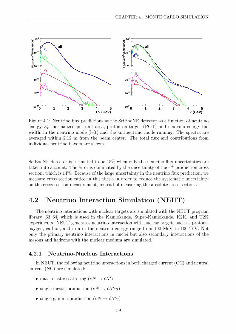
CHAPTER 4. MONTE CARLO SIMULATION
(GeV)νE0 1 2 3 4 5
/25M
eV/P
OT
)2
Flu
x (/
cm
-1410
-1310
-1210
-1110
-1010
-910
allµν
µν
eν
eν
(GeV)νE0 1 2 3 4 5
/25M
eV/P
OT
)2
Flu
x (/
cm
-1410
-1310
-1210
-1110
-1010
-910
all
µν µν
eν eν
Figure 4.1: Neutrino flux predictions at the SciBooNE detector as a function of neutrinoenergy Eν , normalized per unit area, proton on target (POT) and neutrino energy binwidth, in the neutrino mode (left) and the antineutrino mode running. The spectra areaveraged within 2.12 m from the beam center. The total flux and contributions fromindividual neutrino flavors are shown.
SciBooNE detector is estimated to be 15% when only the neutrino flux uncertainties aretaken into account. The error is dominated by the uncertainty of the π+ production crosssection, which is 14%. Because of the large uncertainty in the neutrino flux prediction, wemeasure cross section ratios in this thesis in order to reduce the systematic uncertaintyon the cross section measurement, instead of measuring the absolute cross sections.
4.2 Neutrino Interaction Simulation (NEUT)
The neutrino interactions with nuclear targets are simulated with the NEUT programlibrary [63, 64] which is used in the Kamiokande, Super-Kamiokande, K2K, and T2Kexperiments. NEUT generates neutrino interaction with nuclear targets such as protons,oxygen, carbon, and iron in the neutrino energy range from 100 MeV to 100 TeV. Notonly the primary neutrino interactions in nuclei but also secondary interactions of themesons and hadrons with the nuclear medium are simulated.
4.2.1 Neutrino-Nucleus Interactions
In NEUT, the following neutrino interactions in both charged current (CC) and neutralcurrent (NC) are simulated:
• quasi-elastic scattering (νN → `N ′)
• single meson production (νN → `N ′m)
• single gamma production (νN → `N ′γ)
39

CHAPTER 4. MONTE CARLO SIMULATION
• coherent π production (ν12C(or56Fe) → `π 12C(or56Fe))
• deep inelastic scattering (νN → `N ′hadrons)
where N and N ′ are the nucleons (proton or neutron), ` is the lepton, and m is the meson.Figure 4.2 shows neutrino-nucleus cross sections per nucleon divided by neutrino energy.The expected number of νµ interactions in the SciBar fiducial volume at SciBooNE issummarized in Table 4.1.
(GeV)νE0 1 2 3 4 5
)-1
GeV
2 c
m-3
8 /
E (
10σ
0
0.5
1
(GeV)νE0 1 2 3 4 5
)-1
GeV
2 c
m-3
8 /
E (
10σ
0
0.5
1
Total (CC + NC)
CC total
CC-QE
πCC-resonant
πCC-coherent
DIS)π(include CC-multi
Figure 4.2: Neutrino-nucleus cross sections per nucleon divided by neutrino energy.
Table 4.1: The expected number and fraction of events in each neutrino interaction es-timated by NEUT at the SciBooNE detector location with the neutrino beam exposureof 0.99 × 10²⁰ protons on target. The 10.6 ton fiducial volume of the SciBar detector isassumed. The CC and NC interactions are abbreviated as CC and NC, respectively.
Interaction Type # Events Fraction(%)CC quasi-elastic 53,363 41.4CC single π via resonances 29,688 23.1CC coherent π 1,771 1.4CC single meson except π 839 0.7CC DIS 6,074 4.7NC elastic 22,521 17.5NC single π0 via resonances 6,939 5.4NC coherent π0 1,109 0.9NC single meson except π0 4,716 3.7NC DIS 1,768 1.4
40

CHAPTER 4. MONTE CARLO SIMULATION
Quasi-elastic Scattering
The dominant interaction in the SciBooNE neutrino energy range is quasi-elastic scat-tering. For the quasi-elastic scattering, the formula by Llewellyn-Smith [65] is used inNEUT. The amplitude of this process is described by the product of the leptonic andhadronic weak currents. The hadronic current is expressed as
< N ′|Jhadµ |N >= cos θcu(N ′)
[γµF
1V (Q2) +
iσµνqνξF 2
V (Q2)
2mN
+ γµγ5FA(Q2)
]u(N) , (4.3)
where θc is the Cabbibo angle, ξ ≡ µp − µn = 3.71 is the difference of anomalous dipolemoments between a proton and a neutron, and mN is the nucleon mass. The vector formfactors, F 1
V and F 2V , are represented as
F 1V (Q2) =
(1 +
Q2
4m2N
)−1 [GV
E(Q2) +Q2
4m2N
GVM(Q2)
], (4.4)
ξF 2V (Q2) =
(1 +
Q2
4m2N
)−1 [GV
M(Q2) − GVE(Q2)
], (4.5)
where GVE and GV
M are the electric and magnetic Sachs form factors, given by
GVE(Q2) =
1(1 + Q2
MQEV
2
)2 , GVM(Q2) =
1 + ξ(1 + Q2
MQEV
2
)2 . (4.6)
The axial-vector form factor, FA, is given by
FA(Q2) =gA(
1 + Q2
MQEA
2
)2 , (4.7)
where gA = −1.23 is determined from neutron decay measurements. Both the vectorand axial-vector form factors are assumed to be dipole. The vector mass (MQE
V ) and theaxial vector mass (MQE
A ) for the quasi elastic scattering are set to be 0.84 GeV/c2 and1.21 GeV/c2, respectively, as suggested by recent results [66,67].
The differential cross section is expressed as
dσ
dQ2=
m2NG2
F cos2 θc
8πE2ν
[A(Q2) ∓ B(Q2)
s − u
m2N
+ C(Q2)(s − u)2
m4N
], (4.8)
where Eν is the incident neutrino energy, s − u ≡ 4mNEν − Q2 − m2` , m` is the mass of
the outgoing lepton, and
A(Q2) =m2
` + Q2
4m2N
[(4 +
Q2
m2N
)|FA|2 −
(4 − Q2
m2N
)|F 1
V |2
+Q2
m2N
|ξF 2V |2(
1 − Q2
4m2N
)+
4Q2F 1V ξF 2
V
m2N
− m2`
m2N
(|F 1
V + ξF 2V |2 + |FA|2
)], (4.9)
B(Q2) = − Q2
m2N
FA
(F 1
V + ξF 2V
), (4.10)
C(Q2) =1
4
(|FA|2 + |F 1
V |2 +Q2
m2N
∣∣∣∣ξF 2V
2
∣∣∣∣2)
. (4.11)
41

CHAPTER 4. MONTE CARLO SIMULATION
To obtain the cross sections for neutral current elastic scattering, we use the followingrelations [68,69]:
σ(νp → νp) = 0.153 × σ(νn → µ−p) , (4.12)
σ(νp → νp) = 0.218 × σ(νp → µ+n) , (4.13)
σ(νn → νn) = 1.5 × σ(νp → νp) , (4.14)
σ(νn → νn) = 1.0 × σ(νn → νn) . (4.15)
For scattering off nucleons in the nucleus, we use the relativistic Fermi gas model ofSmith and Moniz [70]. The nucleons are treated as quasi-free particles and the Fermimotion of nucleons along with the Pauli exclusion principle is taken into account. Themomentum distribution of the target nucleon is assumed to be flat up to a fixed Fermisurface momentum of 217 MeV/c for carbon and 250 MeV/c for iron. The same Fermimomentum distribution is also used for all of the other nuclear interactions. The nuclearpotential is set to 27 MeV for carbon and 32 MeV for iron.
Single Meson Production via Baryon Resonances
The second most probable interaction in SciBooNE is the resonant single meson pro-duction of π, K, and η, described by the model of Rein and Sehgal [18]. The main signalin this analysis is NC single π0 production via baryon resonances. The model assumes anintermediate baryon resonance, N∗:
νN → `N∗ ,
N∗ → N ′m (m = π, η, K) . (4.16)
The double differential cross section of single meson production depends on the amplitudefor the production of a given resonance and the probability of the baryon resonance decayto the meson:
d2σ
dQ2dν=
1
32πmNE2ν
· 1
2
∑spins
|T (νN → `N∗)|2 · δ(W 2 − M2) , (4.17)
where W is the hadronic invariant mass and T (νN → `N∗) is given as
T (νN → `N∗) = −4GF cos θcME[
√−q2
Q2< N∗|uF− − vF+|N >
+mN
M
√2uv < N∗|F0|N >]. (4.18)
Here, u and v are defined as
u =E + E ′ + Q
2Ev =
E + E ′ − Q
2E(4.19)
where the incident and final lepton energies are denoted by E and E ′, respectively, and Qis the modulus of the three momentum transfer in the Lab. We use FKR (Feynman-Kislinger-Ravndal) baryon model [71] to express the baryon state (|N >, |N∗ > inEq. 4.18) and calculate F±, F0 in Eq 4.18.
42

CHAPTER 4. MONTE CARLO SIMULATION
In this model, for the baryon of three quarks, we have the SU(6) spin and flavormultiplets (56, 70 and 20) and spatial excitations of two independent three-dimensionalmodes of internal harmonic oscillation among the three particles. Therefore, baryon stateis generally expressed as∑
i
αi|f1, f2, f3 >i |s1, s2, s3 >i |n(space) >i (4.20)
where, fj and sj represent the flavor and spin of the j-th quark, respectively, and|n(space) > is the spatial wave function at the n-th excitation. The way to obtain theexplicit form of Eq. 4.20 for each baryon is described in the Appendix of [71].
To calculate F±, F0 in Eq 4.18, the four-dimensional harmonic oscillator Hamiltonianis used. We just put results here without the details of calculations. For the chargedcurrent, they obtained
FCC± = −9τ+[(T V ±TA)a∓ + (RV ±RA)σ±]e−λaz (4.21)
FCC0 = 9τ+[S + Cσz + B~σ·~a]e−λaz . (4.22)
For the neutral current, they obtained
FNC± = −9
τ 3
2[(T V ±TA)a∓ + (RV ±RA)σ±]e−λaz
− 9 sin2 θw(τ 3 + 1)(T V a∓ + RV σ±)e−λaz (4.23)
FNC0 = 9
τ 3
2[S + Cσz + B~σ·~a]e−λaz
− 9 sin2 θw(τ 3 + 1)Se−λaz . (4.24)
Here the isospin operator (t+, t3), spin operator (1, ~σ) and oscillator operators (~a) act onthe flavor, spin and space sectors in the baryon wave function (Eq. 4.20), respectively,and other parameters are defined as
λ =
√2
Ω
mN
WQ, (4.25)
T V =1
3W
√2
ΩGV (q2), (4.26)
RV =√
2mN
W
(W + mN)Q
(W + mN)2 − q2GV (q2), (4.27)
S = − q2
Q2
3mN + q2 − m2N
6m2N
GV (q2), (4.28)
TA =1
2
√2
Ω
mN
W
Q
(W + mN)2 − q2GA(q2), (4.29)
RA =
√2
8W(W + mN +
2nΩW
(W + mN)2 − q2)GA(q2), (4.30)
B =1
4W
√2
Ω(1 +
W 2 − m2N + q2
(W + mN)2 − q2)GA(q2), (4.31)
C =1
8mNQ(W 2 − m2
N + nΩW 2 − m2
N + q2
(W + mN)2 − q2)GA(q2). (4.32)
43

CHAPTER 4. MONTE CARLO SIMULATION
The transition form factors GV,A(q2) are expressed as
GV,A(q2) = (1 − q2
4m2N
)1/2−n(1
1 − q2/M1πV,A
2 )2 (4.33)
where n is the number of excitations of baryon spatial wave function (Eq. 4.20). Both thevector and axial-vector form factors are assumed to be dipole. The vector mass (M1π
V )and axial vector mass (M1π
A ) for the single meson production, is set to be 0.84 GeV/c2
and 1.21 GeV/c2, respectively.For resonances with a finite decay width, the double differential cross sections can be
derived by replacing the δ-function with a Breit-Wigner formula:
δ(W 2 − M2) → 1
2π
Γ
(W − M)2 + Γ2/4. (4.34)
All intermediate baryon resonances with mass less than 2 GeV/c2 are included. Thosebaryon resonances with mass greater than 2 GeV/c2 are simulated as deep inelastic scat-tering. Lepton mass effects from the non-conservation of lepton current and the pion-poleterm in the hadronic axial vector current are included in the simulation [72,73].
To determine the angular distribution of a pion in the final state, Rein’s method [74]is used for the P33(1232) resonance. For other resonances, the directional distributionof the generated pion is set to be isotropic in the resonance rest frame. The angulardistribution of π+ has been measured for νµp → µ−pπ+ [75] and the results agree wellwith the prediction of NEUT. Pauli blocking is accounted for in the decay of the baryonresonance by requiring the momentum of the nucleon to be larger than the Fermi surfacemomentum. Pion-less ∆ decay is also taken into account, where 20% of the events do nothave a pion and only the lepton and nucleon are generated [76].
Coherent Pion Production
The model of Rein and Sehgal [32, 35] is used to simulate coherent pion productionin NEUT. Based on Adler’s PCAC theorem, the differential cross section for Q2=0 isexpressed as
d3σ(νA → νAπ)
dxdydt
∣∣∣∣Q2=0
=G2
F
π2f 2
πmNEν(1 − y)σ(πA → πA)
dt
∣∣∣∣Eνy=Eπ
, (4.35)
where x = Q2/2mNν and y = ν/Eν are the Bjorken kinematic variables, ν is the energytransfer, t is the square of the four-momentum transferred to the nucleus, GF is the weakcoupling constant, fπ is the pion decay constant, and mN is the mass of nucleon. Therelation expresses the forward neutrino cross section at the nucleus A in terms of the crosssection for the process πA → πA.
The extrapolation of the cross section to Q2 6= 0 is done based on the method of hadrondominance, which is an extension of the model used in electromagnetic interactions, thevector meson dominance (VMD) model. The VMD model treats the electromagneticcurrent as a superposition of the contribution from the lightest vector mesons. Followingthe calculation of the VMD model, the cross section is then obtained by attaching apropagator term:
d3σ(νA → νAπ)
dxdydt=
G2F
π2f2
πmNEν(1 − y)
(m2
A
Q2 + m2A
)2σ(πA → πA)
dt
∣∣∣∣Eνy=Eπ
(4.36)
44

CHAPTER 4. MONTE CARLO SIMULATION
where mA is the axial vector mass, introduced practically in the propagator.The pion-nucleus differential cross section is expressed as
dσ(πA → πA)
dt= A2|FA(t)|2 dσ(πN → πN)
dt
∣∣∣∣t=0
(4.37)
where A is the atomic number of the nucleus, FA(t) is the nuclear form factor (includingthe effect of pion absorption). With the aid of the optical theorem, the pion-nucleondifferential cross section in the forward direction is given by
dσ(πN → πN)
dt
∣∣∣∣t=0
=1
16π
[σπN
tot
]2(1 + r2), r =
Re fπN(0)
Im fπN(0). (4.38)
An average cross section from measurements of pion-deuteron scattering is used to obtainσπN
tot in this model. For the nuclear form factor,
|FA(t)|2 = e−b|t|Fabs (4.39)
is used, where b is related to the nuclear radius R, given by
b =1
3R2 (R = R0A1/3) . (4.40)
The Fabs is the attenuation factor representing the effect of pion absorption in the nucleus,expressed as
Fabs = e−〈x〉/λ , (4.41)
where 〈x〉 and λ are the average path length traversed by the pion produced in the nucleus,and the absorption length, respectively. By assuming the nucleus is a homogeneous spherewith an uniform density, 〈x〉 and λ are calculated as
〈x〉 =3
4R , λ = A
(4πR3
3
)−1
σπNinel , (4.42)
where σπNinel is the pion-nucleon inelastic cross section. As a result of this,
Fabs = exp
(− 9A1/3
16πR20
σπNinel
)(4.43)
is obtained. Hence, the differential cross section for coherent pion production in the modelof Rein and Sehgal is expressed as
d3σ(νA → νAπ)
dxdydt=
G2F
π2f 2
πmNEν(1 − y)
(m2
A
Q2 + m2A
)2 A2
16π
[σπN
tot
]2(1 + r2)e−b|t|Fabs .
(4.44)The Rein and Sehgal model predicts three features of coherent pion production as
follows
1. Since the axial parts of the neutral and charged currents form a triplet in isospace,we are led to f 2
π0 = (√
1/2fπ+)2 = (1/2)f2π+ = (1/2)(0.93mπ)2. Therefore, the
model predicts the relation between the neutral and charged current coherent pionproduction cross sections as σ(CC) = 2 × σ(NC). The relation is slightly modifiedsince the charged current cross section is modified by the lepton mass correction [35].
45

CHAPTER 4. MONTE CARLO SIMULATION
2. The A dependence of the cross section turns out to be approximately A1/3. Thebehavior results roughly from a product A4/3b−1b−1/2, where b ∼ R2 ∼ A2/3. Thefirst factor is the effect of nuclear coherence, including the effects of pion absorption,the second factor comes from integration of e−b|t| over t, the third one comes fromintegration over x.
3. The model predicts the same cross section for coherent pion production by neutrinosand antineutrinos.
In our MC simulation, we set the axial vector mass, mA, to 1.0 GeV/c2, and thenuclear radius parameter, R0, is set to 1.0 fm. For the total and inelastic pion-nucleoncross sections, σπN
tot and σπNinel, respectively, the fitted results given in Rein and Sehgal’s
paper are used.
Deep Inelastic Scattering (DIS)
The double differential cross section for charged current deep inelastic scattering (DIS)is calculated as:
d2σ
dxdy=
G2F mNEν
π
[(1 − y +
1
2y2 + C1
)F2(x) ± y
(1 − 1
2y + C2
)xF3(x)
],(4.45)
C1 =m2
`(y − 2)
4mNEνx− mNxy
2Eν
− m2`
4E2ν
, (4.46)
C2 = − m2`
4mNEνx, (4.47)
where x ≡ Q2/(2mN(Eν − E`) + m2N) and y ≡ (Eν − E`)/Eν are the Bjorken scaling
parameters, and E` is the energy of the final state lepton. The nucleon structure func-tions, F2 and xF3, are calculated using the GRV98 parton distribution functions [77]. Inaddition, we have included the corrections in the small Q2 region developed by Bodek andYang [78]. In the calculation, the hadronic invariant mass, W , is required to be largerthan 1.3 GeV/c2.
The multi-hadron final states are simulated with two models. In the range of 1.3 <W < 2.0 GeV/c2, a custom-made program [79] is employed. For the events with W >2 GeV/c2, PYTHIA/JETSET [80] is used to calculate the kinematics of hadronic finalstates.
To obtain the cross sections for neutral current deep inelastic scattering, we use thefollowing relations:
σ(ν NC-DIS)
σ(ν CC-DIS)=
0.26 (Eν ≤ 3 GeV)0.26 + 0.04 × (Eν/3 − 1) (3 < Eν < 6 GeV)0.30 (Eν ≥ 6 GeV)
, (4.48)
σ(ν NC-DIS)
σ(ν CC-DIS)=
0.39 (Eν ≤ 3 GeV)0.39 − 0.02 × (Eν/3 − 1) (3 < Eν < 6 GeV)0.37 (Eν ≥ 6 GeV)
. (4.49)
These relations are estimated from the experimental results [81,82].
46

CHAPTER 4. MONTE CARLO SIMULATION
4.2.2 Intra-nuclear Interactions
The interactions of mesons and nucleons produced via neutrino interactions with nu-clear matters are simulated. These interactions are treated by using a cascade model,and each of the particles is traced until it escapes from the nucleus. The neutrino inter-action position in the nucleus is calculated using the Wood-Saxon type nucleon densitydistribution:
ρ(r) =Z
Aρ0
[1 + exp
(r − c
a
)]−1
, (4.50)
where ρ0 = 0.48m3π, A and Z are the mass number and atomic number of the nucleus,
respectively. For carbon nucleus, a = 0.52 fm and c = 2.36 fm [83]. Fermi motion ofnucleons in the nucleus and Pauli blocking effect are taken into account in the simulation.The Fermi surface momentum at the interaction point is defined as
pF (r) =
(3
2π2ρ(r)
) 13
. (4.51)
Pion Interactions
The interactions of pions are most important for the analysis in this thesis. The inelas-tic scattering, charge exchange and absorption of pions in the nuclei are simulated. Theinteraction cross sections of pions in the nuclei are calculated using the model by Salcedoet al. [84], which agrees well with past experimental data [85]. If inelastic scattering orcharge exchange occurs, the direction and momentum of pions are determined by usingresults from a phase shift analysis of pion-nucleus scattering experiments [86].
In SciBooNE, approximately 15% of pions produced via neutrino interaction are ab-sorbed in carbon, about 20% of pions are inelastically scattered, and the probability ofcharge exchange is 5%.
Nucleon Re-scattering
Re-interactions of the recoil protons and neutrons produced in neutrino interactions arealso simulated. Nucleon-nucleon interactions modify the outgoing nucleon’s momentumand direction. Both elastic scattering and pion production are considered. The differentialcross sections were obtained from nucleon-nucleon scattering experiments [87]. For pionproduction, the isobaric nucleon model [88] is used.
In SciBooNE, approximately 35% of protons produced via charged current quasi-elasticscattering interact inside of the carbon nucleus.
4.3 Detector Simulation
We use the GEANT4 framework for the detector simulation. The detector simulationincludes a detailed information of the detector geometry.
4.3.1 Simulation of Detector Responses
In the detector simulation of SciBar, true energy deposition in a scintillator stripssimulated by GEANT is converted to the number of photoelectrons using a conversion
47

CHAPTER 4. MONTE CARLO SIMULATION
factor which is measured for each channel with cosmic-ray muons. Scintillator quenchingis simulated using Birk’s law with a measured value of Birk’s constant. [54] The measuredlight attenuation length (Table 3.1) of each fiber is used in the simulation. Crosstalkbetween nearby MA-PMT channels is simulated using measured values (Table 3.1). Tosimulate the digitization of the PMT signal, the number of photoelectrons is smeared byPoisson statistics and by the PMT resolution, and then converted to ADC counts. Alogical OR of 32 MA-PMT channels is made for each TDC channel, and the time of eachhit is converted to TDC counts. Multiple TDC hits in each channel are simulated.
In the EC detector simulation, true energy deposition in scintillating fibers in thedetector is converted to the number of photoelectrons using a conversion factor whichis measured for each channel with cosmic-ray muons. The attenuation of light in thefiber is simulated using the measured attenuation length value (400 cm). The numberof photoelectrons is smeared by Poisson statistics and by the PMT resolution, and thenconverted to ADC counts.
For the detector simulation of the MRD, true energy deposition in each scintillator isconverted to ADC counts using the conversion factor measured with cosmic muons. Theattenuation of light in the scintillator are simulated. Gaps between scintillator countersin each plane, which cause inefficiency (1 %), are included in the simulation. The time ofenergy deposition is digitized and converted into TDC counts.
In addition to the main components such as SciBar, EC and MRD, the particle trans-portation in the detector structure frame made of iron and the dark box made of wood isalso simulated.
4.3.2 Simulation of Pion Interaction in Detector
The Bertini cascade model within GEANT4 [89] is used to simulate the interactionsof hadrons with detector materials. Among all the hadronic interactions, the interactionsof pions are most important to the analysis. To check the validity of the simulationin our interested energy region (Tπ < 500 MeV), the simulated cross section of pion-carbon interaction is compared with external measurements [85, 90–94]. As a result, a10% difference of the total cross section between the MC simulation and data is seen forhigher energy pion. The difference is accounted for when we evaluate systematic errors.
4.3.3 Neutrino Interactions in the Surrounding Material
In addition to neutrino interactions inside the detector, we also simulate interactionsin the surrounding material (the walls of the detector hall and soil). The density ofmaterial is assumed to be 2.15 g/cm3 for the calculation of the interaction rate. Theconcrete material with the density of 2.15 g/cm3 is used as the material for propagationof product particles. We generate events in a volume of ±5 m in x, y, and z direction inthe SciBooNE coordinates. The details are described in Appendix B.
48

Chapter 5
Event Selection for Neutral Currentπ0 Production
5.1 Overview
As shown in Table 4.1, the fraction of NCπ0 production to all neutrino interactions isonly about 6 %. Hence, we need make NCπ0 enriched sample by applying the selections.In this chapter, we describe the event selections in detail.
Figure 5.1 shows the event display of typical NCπ0 candidate in SciBooNE. We aim toreconstruct and select events where NCπ0 interaction is occurred inside SciBar detectorand both two gamma rays from π0 are converted into e+e− pairs also in SciBar. Thedetail of the NCπ0 signal definition is described in Section 5.2.
Before we describe the NCπ0 event selections, we describe the particle reconstructionin Section 5.3. This is because the reconstructed objects such as hits, clusters and tracksare used for the event selections. As shown in this chapter, we keep gamma ray tracksby removing the proton and muon tracks because most of particles making tracks inSciBar are protons or muons except for gamma rays. In addition, identifying the muonsis important to reject the CC background events. Furthermore, as shown in Figure 5.1, asingle gamma ray in SciBooNE energy range (a few hundred MeV) makes one main trackand additional hits or short tracks around the main track in SciBar. Therefore, we performthe track-based reconstruction, which is commonly used for all SciBooNE analyses. Then,we identify protons and muons using the reconstructed tracks. The reconstructed tracksis also used for the reconstruction of gamma rays and π0.
We also describe CC sample in Section 5.4. The CC sample is used for the beamflux normalization. Finally, we present the event selections for the NCπ0 production inSection 5.5
5.2 Signal Definition
We define an NCπ0 interaction as an NC neutrino interaction in which at least one π0
is emitted in the final state from the target nucleus, νµC → νµπ0X where X represents
the nuclear remnant and any combination of nucleons and mesons. We include suchNCπ0 interactions occurring only in SciBar as our signals. Unless otherwise indicated,our “NCπ0” means a NCπ0 interaction occurring in SciBar but neither in EC nor MRD.
49

CHAPTER 5. EVENT SELECTION FOR NEUTRAL CURRENT π0 PRODUCTION
Figure 5.1: Event display of a typical NCπ0 event candidate in SciBooNE data. Theneutrino beam runs from left to right in this figure, encountering SciBar, the EC andMRD, in that order. The circles on SciBar indicate ADC hits for which the area of thecircle is proportional to the energy deposition in that channel. This event display showsthe electromagnetic shower tracks from the pair conversions of the two π0 decay photons.
According to our MC simulation, 96% of NCπ0 events without any selection cuts havea single π0 (85 % from a single π0 without any other mesons and 11 % from a singleπ0 with charged mesons) and 4 % have two π0s. Any π0 emitted from the initial targetnucleus constitutes a signal event whether it is created from the neutrino vertex or finalstate interactions. Events with a π0 produced in the neutrino interaction but absorbedin the target nucleus are not included in the signal sample, nor are events in which π0sare produced by secondary particles interacting with the detector scintillator outside thetarget nucleus. We show the classification of the NCπ0 signal and non-signal in Figure 5.2.
We identify π0 by two reconstructed gamma rays. Hence, both of the two gammarays from π0 must be converted into e+e− pairs in SciBar to be identified as a π0 events.In fact, the number of signal events where both of the two gamma rays are convertedin SciBar is only 30 % of all signals. This means that the maximum NCπ0 detectionefficiency attainable is 30 %. We will describe the gamma conversion probability in detailin Section 6.6.2.
50

CHAPTER 5. EVENT SELECTION FOR NEUTRAL CURRENT π0 PRODUCTION
target nuclear
neutrino
neutral pion
target nuclear
neutrinocharged pion
neutral pion
Signal
(b) (c)
target nuclear
neutrinoneutral pion
target nuclear
neutrino
charged pion
other nuclear
neutral pion
nuclear effect (charge exchange) multi pion
(d) nuclear effect (absorption) (e) secondary production in detector
(a) primary pi0 production
target nuclear
neutrino
neutral pion
neutral (charged) pion
Not signal
Figure 5.2: Classification of the NC π0 signal and non-signal
5.3 Particle Reconstruction
5.3.1 Overview
Figure 5.3 shows a schematic view of the event reconstruction of SciBooNE. In SciBar,hits and 2D tracks, 3D tracks (we call just “tracks” hereafter) are obtained described asSection 5.3.2. In this analysis, 2D projections are used only for reconstructing tracksnot directly used for the event selections or π0(γ) reconstruction. Based on the dE/dxinformation, SciBar tracks are divided into proton-like tracks or non-proton-like tracksas described in Section 5.3.3. For the gamma ray reconstruction, extended tracks areobtained after the additional treatment to the non-proton-like tracks as described inSection 5.3.4.
The EC information are obtained as hits and clusters. We search the EC clustersmatching with the tracks as described in Section 5.3.5. Such matched EC clusters areused for the muon identification and energy correction for gamma rays.
The MRD information are obtained as hits and tracks. We search the MRD hits ortracks matching with the SciBar tracks as described in Section 5.3.6. Such SciBar-MRDmatched tracks are used for the muon identification.
5.3.2 SciBar Track Reconstruction
The first step of the SciBar event reconstruction is to search for two-dimensionaltracks in each view of SciBar using a cellular automaton algorithm [95]. For tracking, the
51

CHAPTER 5. EVENT SELECTION FOR NEUTRAL CURRENT π0 PRODUCTION
2D projection
Hit
Track
2D projection
Track
Hit
Cluster
Hit
Non−proton−like track
SciBar−EC matching
SciBar−MRD matching
Proton−like track
Hit collectionTrack merge
Extended track
2D projection search2D projection search
2D projection match
SciBarMRD EC
Particle identification
Continuous hits search
2D projection match
2D projection search
Figure 5.3: The schematic view of the event reconstruction of SciBooNE
hit threshold is set to 2.5 photo-electrons, corresponding to roughly 0.25 MeV.∗ Threedimensional tracks are reconstructed by matching the timing and z-edges of the twodimensional projections. In order to match track projections in a three dimensional track,the timing difference between two two-dimensional projections is required to be less than50 ns, and the z-edge difference must be less than 6.6 cm for upstream and downstreamedges.
∗The previous SciBooNE result such as the measurement of charged current coherent production[56] used 2.0 photo-electrons threshold. We noticed that the data/MC discrepancies of the gamma rayreconstructions such as energy, direction and number of collected hits are large around 2.0 photo-electronsthreshold. Hence, we decided to use 2.5 photo-electrons threshold.
52

CHAPTER 5. EVENT SELECTION FOR NEUTRAL CURRENT π0 PRODUCTION
5.3.3 Particle Identification Parameter
The SciBar detector has the capability to distinguish protons from other particles byusing dE/dx since the energy deposit of recoil protons at SciBooNE energies is largerthan minimum ionizing energy deposit. We define a muon confidence level (MuCL) usingthe observed energy deposit per layer for all reconstructed tracks [49]. The MuCL ofthe proton tracks tends to be close to 0 while the MuCL of other tracks tends to beclose to 1. Figure 5.4 shows the distribution of the MuCL. For the MC simulation, thecontribution from gamma rays, muons, protons and other particles are separately shown,respectively. Tracks with MuCL less than 0.03 are called proton-like tracks, otherwisecalled non-proton-like tracks.
Figure 5.4: Distribution of MuCL of tracks
5.3.4 Extended Track
As mentioned at the beginning of this chapter, the typical gamma rays make one maintrack and additional short tracks or hits around the main track in SciBar. To reconstructthe energy of gamma rays, we need to collect such additional hits and short tracks. Incase of additional short tracks, we need to relate the short tracks to the main track andhandle them as a single gamma ray not two different particles. Hence, we introduce newreconstructed tracks called “extended tracks” based on the original reconstructed tracks.
Reconstructed tracks are extended in two ways to improve energy reconstruction ofgamma rays within SciBar. The first step is merging two or more tracks if they arenearly co-linear, because electromagnetic showers can form separate hit clusters in SciBarresulting in two or more tracks. The second step is collecting hits around merged tracks.Electromagnetic showers sometimes deposit energy around the main track and these hitsare missed by the track reconstruction algorithm. Hits within 20 cm from 2D projectionsof the merged track (i.e., after the first step) for each view but not assigned to anytrack are added to the extended track. The methods described above are applied onlyto non-proton-like tracks. For the energy reconstruction, we use charge information ofhits associated with original tracks as well as newly assigned hits. For reconstructing the
53

CHAPTER 5. EVENT SELECTION FOR NEUTRAL CURRENT π0 PRODUCTION
directions of gamma rays, we fit positions of hits in all original tracks in the extendedtrack with a straight line and do not use hits newly collected in the second step. Thedetails of the extended track is described in Appendix. A.
5.3.5 SciBar-EC Matching
Some particles can escape SciBar and deposit energy in the EC. After event recon-struction in SciBar we search for EC clusters aligned with tracks from SciBar. One ECcluster is defined as a collection of neighboring EC hits. For an EC hit, the pulse heightsof both side PMTs are required to be above threshold, which is set to 3 times the width ofeach pedestal—about 7 MeV. The energy of an EC hit is the geometric average of the twoPMTs. The center of an EC cluster is defined as the energy-weighted average of hits inthe cluster. To match the EC cluster to the SciBar track, the EC cluster is required to bewithin 10 cm of the extrapolated two-dimensional projections of the SciBar track in eachEC plane. The energy of matched EC clusters is added to the corresponding extendedtracks. The details of the SciBar-EC matching is described in Appendix. A.
5.3.6 SciBar-MRD Matching
A track in SciBar matched to a track or hits in MRD is called the SciBar-MRDmatched track. For matching the MRD track to a SciBar track, the upstream edge of theMRD track is required to be on either one of the first two layers of MRD. The transversedistance between the two tracks at the first layer of MRD must be less than 30 cm. Therequirement on the difference between track directions is given by |θMRD − θSB| < θmax,where θmax is a function of the length of the MRD track in the range between 0.4 radianand 1.1 radians. If no MRD track is found, we extrapolate the SciBar track to the MRDand search for nearby contiguous hits in MRD. For matching MRD hits to the SciBartrack, the MRD hit is required to be within a cone with an aperture of ± 0.5 radian anda transverse offset within 10 cm of the extrapolated SciBar track at the upstream edge ofMRD. The timing difference between the SciBar track and the track or hits in MRD isrequired to be within 100 nsec.
5.4 MC Normalization (Charged-Current Event Sam-
ple)
To identify charged current events, we search for events with at least one SciBar-MRD matched track. We reject events with hits associated with the muon track on themost upstream layer of SciBar to eliminate neutrino-induced incoming particles from theupstream wall or soil. The neutrino interaction vertex for CC events is reconstructed asthe upstream edge of the muon track. We select events whose vertices are in the SciBarfiducial volume. The fiducial volume is defined as
−130 cm < x < 130 cm−130 cm < y < 130 cm2.62 cm < z < 157.2 cm (2nd − 60th layer)
(5.1)
The total mass in the fiducial volume is 10.6 tons. The time of the muon track is requiredto be within a 2 µs window around the beam pulse. Finally, we require the muon track to
54

CHAPTER 5. EVENT SELECTION FOR NEUTRAL CURRENT π0 PRODUCTION
stop in the MRD. The MRD-stopped event sample [49] serves as the normalization samplein the cross-section ratio measurement. Unless otherwise indicated, the MC distributionsin this paper are normalized by using the MRD-stopped data sample.
5.5 Event Selection for NCπ0
5.5.1 Overview
The clear feature of NC π0 production is two gamma rays, coming from the decay of theπ0, converted into two e+e− pairs. Background events can be categorized into two types.One is called an internal background. Internal backgrounds are neutrino interactionsother than NCπ0 (mainly CC) within SciBar. The other is called an external background.External backgrounds come from neutrino interactions in the material outside of thedetector volume (support structure, walls and soil—so called dirt background events) aswell as from cosmic rays. In dirt background events, neutrinos interact with materialssuch as the walls of the experimental hall or soil and produce secondary particles whichdeposit energy within SciBar’s fiducial volume. The contribution of accidental cosmicrays in the event samples is small and accurately estimated by data taken with off-beamtiming; the fraction of accidental cosmic ray events is 1.8% after all event selection cuts.Data distributions shown hereafter are after subtracting the cosmic backgrounds. Theevent selection cuts for NCπ0 production are developed to select events with two gammarays while rejecting the above background events.
The event selection cuts are summarized as follows.
(1) Number of tracks
(2) Fiducial volume cut
(3) First layer veto
(4) Side escaping track rejection cut
(5) Decay electron rejection cut
(6) Track disconnection cut
(7) Electron catcher cut
(8) Number of extended tracks
(9) π0 vertex cut
(10) π0 mass cut
Here, we describe the outline of the event selection cuts. We describe the details of eachcuts in following selections. First, at least two tracks starting in SciBar are selected atthe selections (1)(2). Charged particles from the outside of SciBar are rejected at theselection (3). Muons escaping from the side of SciBar or stopping in SciBar are rejectedat the selections (4)(5). At the selection (6), we reject charged current events with twoparticles whose vertices are common. For selections (1)-(6), we use information from only
55

CHAPTER 5. EVENT SELECTION FOR NEUTRAL CURRENT π0 PRODUCTION
SciBar. At the selection (7), we use EC to reject muons going though SciBar. At theselection (8)(9)(10), we select two gamma rays from π0s and reject gamma ray enteringfrom the outside of SciBar. We use standard tracks for selections (1)-(7) since their mainpurpose is charged current rejection. For selections (8)(9)(10), we use extended trackssince their main purpose is selecting two gamma rays or rejecting gamma rays from theoutside of SciBar.
5.5.2 Number of Tracks
To find two gamma rays, we select events with at least two tracks whose timingdifference is less than 50 ns. Figure 5.5 shows the number of tracks distribution after theselection.
Number of tracks
En
trie
s
0
10000
20000
Number of tracks
En
trie
s
0
10000
20000
Data
0πNC
0πInt. BG with
0πInt. BG without
Dirt
22 3 4 5 61
Figure 5.5: The number of tracks distribution; The MC contribution from the NCπ0, theinternal background with π0s in the final state, the internal background without π0s inthe final state and the dirt background events are shown separately.
5.5.3 Fiducial Volume Cut
There are four track edge combinations in two tracks (Figure 5.6). We calculatethe distance between edges for these four combination and select the one which givesminimum distance; “Closest edges”. In case that two γs are correctly reconstructed astwo tracks, this minimum distance corresponds to the distance between the points where2γs convert to the electromagnetic showers. “Closest edges” of two tracks are required tobe in this fiducial volume defined in Equation 5.1. Figure 5.7 shows the upstream edgeof the longest track after this fiducial volume cut. The discrepancy between data and theMC simulation is seen, especially in the events where the tracks start at the upstream ofSciBar. According to the MC simulation, the main contribution of such events is the dirtbackground events which is not precisely predicted.
56

CHAPTER 5. EVENT SELECTION FOR NEUTRAL CURRENT π0 PRODUCTION
3D Track "1"
3D Track "2"
edge A1
edge A2
edge B1
edge B2
Figure 5.6: There are four edge combinations, which are (A1, B1), (A1, B2), (A2, B1),and (A2, B2). And “Closest edges” are A1 and B1.
Upstream edge position X (cm)-100 0 100
Ent
ries
/ 10c
m
0
500
1000
Upstream edge position X (cm)-100 0 100
Ent
ries
/ 10c
m
0
500
1000
Data
0πNC
0πInt. BG with
0πInt. BG without
Dirt
Upstream edge position Y (cm)-100 0 100
Ent
ries
/ 10c
m
0
500
1000
Upstream edge position Y (cm)-100 0 100
Ent
ries
/ 10c
m
0
500
1000
Data
0πNC
0πInt. BG with
0πInt. BG without
Dirt
Upstream edge position Z (cm)0 100
Ent
ries
/ 5cm
1000
2000
Upstream edge position Z (cm)0 100
Ent
ries
/ 5cm
1000
2000 Data
0πNC
0πInt. BG with
0πInt. BG without
Dirt
Figure 5.7: The upstream edge distribution of the longest track after this fiducial volumecut
5.5.4 First Layer Veto
To reduce dirt background, we reject events with hits in the first layer within 100 nsfrom the timing of tracks. Figure 5.8 shows the upstream edge of the longest track afterthe first layer veto. Figure 5.9 shows the downstream edge of the longest tracks. Thepeak seen at z = 165 cm indicates that many muons (charged current events) go out fromSciBar.
5.5.5 Side Escaping Track Rejection Cut
There are charged current events with muons escaping from the side of SciBar. Toreduce these events, the x and y position of both edges of the tracks are required to be infiducial volume (Figure 5.10). Figure 5.11 and 5.12 shows the upstream and downstreamedge of the longest tracks after the cut, respectively. By this cut, 41 % of the backgroundevents are rejected. Meanwhile, the NCπ0 efficiency of this cut is 77 %.
57

CHAPTER 5. EVENT SELECTION FOR NEUTRAL CURRENT π0 PRODUCTION
Upstream edge position X (cm)-100 0 100
Ent
ries
/ 10c
m
0
500
1000
Upstream edge position X (cm)-100 0 100
Ent
ries
/ 10c
m
0
500
1000 Data
0πNC
0πInt. BG with 0πInt. BG without
Dirt
Upstream edge position Y (cm)-100 0 100
Ent
ries
/ 10c
m
0
500
1000
Upstream edge position Y (cm)-100 0 100
Ent
ries
/ 10c
m
0
500
1000 Data
0πNC
0πInt. BG with 0πInt. BG without
Dirt
Upstream edge position Z (cm)0 100
Ent
ries
/ 5cm
0
500
Upstream edge position Z (cm)0 100
Ent
ries
/ 5cm
0
500
Data
0πNC 0πInt. BG with
0πInt. BG without
Dirt
Figure 5.8: The upstream edge distribution of the longest track after first layer veto
Downstream edge position X (cm)-100 0 100
Ent
ries
/ 10c
m
0
500
Downstream edge position X (cm)-100 0 100
Ent
ries
/ 10c
m
0
500
Data0πNC
0πInt. BG with 0πInt. BG without
Dirt
Downstream edge position Y (cm)-100 0 100
Ent
ries
/ 10c
m
0
500
Downstream edge position Y (cm)-100 0 100
Ent
ries
/ 10c
m
0
500
Data0πNC
0πInt. BG with 0πInt. BG without
Dirt
Downstream edge position Z (cm)0 100
Ent
ries
/ 5cm
210
410
Downstream edge position Z (cm)0 100
Ent
ries
/ 5cm
210
410 Data
0πNC
0πInt. BG with
0πInt. BG without
Dirt
Figure 5.9: The downstream edge distribution of the longest track after the first layerveto
Accept Accept Reject
130 cm
−130 cm
Figure 5.10: Only events with track escaping from the side of SciBar are rejected
58

CHAPTER 5. EVENT SELECTION FOR NEUTRAL CURRENT π0 PRODUCTION
Upstream edge position X (cm)-100 0 100
Ent
ries
/ 10c
m
0
500
Upstream edge position X (cm)-100 0 100
Ent
ries
/ 10c
m
0
500
Data0πNC
0πInt. BG with 0πInt. BG without
Dirt
Upstream edge position Y (cm)-100 0 100
Ent
ries
/ 10c
m
0
500
Upstream edge position Y (cm)-100 0 100
Ent
ries
/ 10c
m
0
500
Data0πNC
0πInt. BG with 0πInt. BG without
Dirt
Upstream edge position Z (cm)0 100
Ent
ries
/ 5cm
0
200
400
Upstream edge position Z (cm)0 100
Ent
ries
/ 5cm
0
200
400
Data
0πNC
0πInt. BG with
0πInt. BG without
Dirt
Figure 5.11: The upstream edge of the longest track after rejecting side escaping tracks
Downstream edge position X (cm)-100 0 100
Ent
ries
/ 10c
m
0
500
Downstream edge position X (cm)-100 0 100
Ent
ries
/ 10c
m
0
500
Data
0πNC 0πInt. BG with
0πInt. BG without
Dirt
Downstream edge position Y (cm)-100 0 100
Ent
ries
/ 10c
m
0
500
Downstream edge position Y (cm)-100 0 100
Ent
ries
/ 10c
m
0
500
Data0πNC
0πInt. BG with 0πInt. BG without
Dirt
Downstream edge position Z (cm)0 100
Ent
ries
/ 5cm
10
210
310
Downstream edge position Z (cm)0 100
Ent
ries
/ 5cm
10
210
310
Data
0πNC 0πInt. BG with
0πInt. BG without
Dirt
Figure 5.12: The downstream edge of the longest track after rejecting side escaping tracks
5.5.6 Decay Electron Rejection Cut
To reject muons stopping in SciBar, we tag the electrons from muon decay. No chargeinformation is recorded for any scintillator strip after the first hit in an event, but the timesof hits above threshold are recorded. Thus most decay electrons are not reconstructed astracks but can be identified as delayed time hits near the end of a muon track. To detectdecay electrons, we use a value called ∆tmax defined as below
1. Find TDC channels corresponding to the upstream and downstream edges of alltracks for both views
2. Among founded TDC channels, choose TDC hits coincident with another viewwithin 50 ns to reduce the accidental noise. Since there are multiple tracks andTDC hits, the number of chosen TDC hits could be more than one.
3. Calculate timing difference between hits at the upstream and downstream. In caseof more than one combination of the upstream and downstream hits due to multipletracks and TDC hits, the difference is calculated for any combinations.
4. Define the maximum one below 5000 ns as ∆tmax.
Events with decay electrons yield large values of ∆tmax because of the long muonlifetime (τµ = 2.2 µ sec) while ∆tmax is less than 10 ns (time that particles transportin SciBar) in case of no decay electron at any edges. Figure 5.13 shows the distributionof ∆tmax. ∆tmax of the most of no decay electron events is less than 100 ns. We reject
59

CHAPTER 5. EVENT SELECTION FOR NEUTRAL CURRENT π0 PRODUCTION
events with ∆tmax greater than 100 ns. By this cut, 31 % of the background events arerejected. Meanwhile, the NCπ0 efficiency of this cut is 94 %.
Figure 5.13: Distribution of ∆tmax;The MC contribution from events with decay electronsin SciBar, events without decay electrons in SciBar and dirt backgrounds, are shownseparately.
5.5.7 Track Disconnection Cut
Charged current events often have multiple tracks with a common vertex while 2γsfrom π0 usually are isolated from each other. The distance between tracks is a good valueto separate the 2γ events from the charged current events. We define “minimum trackdistance” as below
1. Select two tracks
2. Calculate 2D distances for all combination of edges of two tracks.
3. Repeat the same procedure for all combinations of two tracks. We have several 2Ddistances.
4. Define the minimum one as a “minimum track distance”
Figure 5.14 shows the “ minimum track distance”. The contamination of charged currentevents concentrates around zero. We reject events with the minimum track distance lessthan 6 cm.
5.5.8 Electron Catcher Cut
Matched EC clusters are used to reject muons penetrating the EC. Two quantitiesare used: the energy deposit in matched EC clusters in the upstream layer, E1, andthe ratio of energy deposits in the downstream EC cluster (E2) over the upstream EC
60

CHAPTER 5. EVENT SELECTION FOR NEUTRAL CURRENT π0 PRODUCTION
Minimum distance (cm)0 50 100
Ent
ries
/ 2cm
1
10
210
310
Minimum distance (cm)0 50 100
Ent
ries
/ 2cm
1
10
210
310
Data
0πNC
0πInt. BG with
0πInt. BG without
Dirt
Minimum distance (cm)0 10 20
Ent
ries
/ 2cm
0
1000
2000
Minimum distance (cm)0 10 20
Ent
ries
/ 2cm
0
1000
2000Data
0πNC
0πInt. BG with
0πInt. BG without
Dirt
Figure 5.14: Distribution of “minimum track distance” after decay electron rejection. Theright plot is a zoomed-out version of the left plot
cluster, REC = E2/E1. Since muons tend to penetrate more material than γs, the energydeposit of muon at both upstream and downstream planes are close to each other whileγs stop in the short range after conversion with large energy deposit in the upstreamcluster. Figure 5.15 shows scatter plots between E1 and REC for muons and γs in the MCsimulation. The E1 and REC are defined event by event as described below.
(MeV)1E0 200 400
EC
R
0
1
2
3
0
0.2
0.4
0.6
0.8
1
(MeV)1E0 200 400
EC
R
0
1
2
3
0
0.2
0.4
0.6
0.8
1
Figure 5.15: The 2D plots between the E1 and REC for γs (left) and muons (right). Eventswithout any tracks matched to EC clusters are not included in these plots.
1. For events without any tracks matched to EC clusters, both E1 and REC are leftundefined.
2. For events with tracks matched with both upstream and downstream EC clusters,
61

CHAPTER 5. EVENT SELECTION FOR NEUTRAL CURRENT π0 PRODUCTION
the track with maximum energy ratio of the upstream plane to the downstreamplane is selected. The maximum energy ratio is REC. The upstream energy depositin the track is E1.
3. For events with only tracks matched with upstream EC cluster, the track givingminimum upstream energy deposit is selected as E1. REC is 0.
Number of tracks with matched EC clusters0 2 4
En
trie
s
0
2000
Number of tracks with matched EC clusters0 2 4
En
trie
s
0
2000
Data
0πNC
0πInt. BG with
0πInt. BG without
Dirt
Figure 5.16: Option 1 of the EC cut: the number of track with matched EC clusters afterthe track disconnection cut. Events without SciBar-EC matched tracks pass the EC cut.Events with SciBar tracks matching EC clusters can pass the EC cut if they satisfy theOption 2 or Option 3.
Figure 5.16, 5.17 and 5.18 show the number of tracks with matched EC clusters, E1
and REC. Events satisfying at least one of three requirements below are selected
Option 1 There are no tracks matched to the EC clusters.
Option 2 E1 is greater than 150 MeV
Option 3 REC is less than 0.2
By this cut, 28 % of the background events are rejected. Meanwhile, the NCπ0 efficiencyof this cut is 91 %.
5.5.9 The Number of Extended Tracks
After the EC cut, we reconstruct γs to select π0 events and reject γs from the outsideof SciBar. Therefore our event selections are based on “extended track” rather thanthe standard track. As described in Section 5.3.4 the methods for extended tracks areapplied for non-proton-like tracks. Figure 5.19 shows the MuCL distribution after the ECcut. The dashed line (MuCL = 0.03) separates particles to proton-like or non-proton-liketracks. The gamma ray efficiency for the non-proton-like sample is 87 % and the purity
62

CHAPTER 5. EVENT SELECTION FOR NEUTRAL CURRENT π0 PRODUCTION
Figure 5.17: Option 2 of the EC cut: the energy deposited in the upstream layer of theEC (E1) after the track disconnection cut. Events with E1 > 150 MeV pass the EC cut.Events with E1 < 150 MeV can pass the EC cut if they satisfy the Option 3.
Figure 5.18: Option 3 of the EC cut: the ratio of deposited energy in the downstream overthe upstream layer (R) after the track disconnection cut. Only events with E1 < 150 MeVare shown.
of gamma rays in the non-proton-like sample is 81 %. Figure 5.20 shows the number ofnon-proton-like tracks and proton-like tracks.
The contribution from the dirt backgrounds is not negligible after EC cut. About70 % of two tracks in dirt background events are made by single γ from π0 produced inthe outside of the detectors. Since two tracks made by the single γ are nearly co-linear,these tracks become just one extended track by the track merging. Figure 5.21 showsthe number of extended tracks. Many dirt backgrounds are just one extended track asexpected. Events with at least two extended tracks are selected for π0 reconstruction.
63

CHAPTER 5. EVENT SELECTION FOR NEUTRAL CURRENT π0 PRODUCTION
Figure 5.19: Distribution of MuCL of tracks after the EC cut.
Number of non-proton-like tracks0 2 4
Ent
ries
0
1000
2000
Number of non-proton-like tracks0 2 4
Ent
ries
0
1000
2000Data
0πNC
0πInt. BG with
0πInt. BG without
Dirt
Number of proton-like tracks0 2 4
Ent
ries
0
1000
Number of proton-like tracks0 2 4
Ent
ries
0
1000
Data
0πNC
0πInt. BG with
0πInt. BG without
Dirt
Figure 5.20: From the left, the number of non-proton-like tracks and that of proton-liketracks , respectively
As shown in Figure 5.21, 58 % of the NCπ0 signals have only one extended track andrejected by the cut. However, 67% among such rejected NCπ0 signals are events withone reconstructed gamma ray, due to mis-reconstruction or gamma rays not converting inSciBar. Such events can not be used for π0 reconstruction; 21% are events where the twogamma rays are reconstructed as two tracks but one of them is identified as a proton-liketrack; 12% are events in which the two gamma rays are reconstructed as two tracks butthen merged, resulting in one extended track.
5.5.10 π0 Vertex Cut
As described in Section 5.5.9, the events with single γ from the outside of the detectorsare main contribution to dirt background events and such dirt background events are
64

CHAPTER 5. EVENT SELECTION FOR NEUTRAL CURRENT π0 PRODUCTION
Figure 5.21: The number of extended tracks after the EC cut
rejected by selecting events with at least two extended tracks. After selecting events withat least two extended tracks, the dirt background events have 2γs from π0. We rejectsuch dirt background events by reconstructing the π0 vertex. We reconstruct π0 vertexin the following way.
1. Fit extended tracks for both views with linear function as below.
x = atopz + btop (5.2)
y = asidez + bside, (5.3)
where (atop, btop) and (aside, bside) are fitting parameters of the linear function forthe top view and side view, respectively.
2. Calculate the intersection of two extended tracks for each view. (zx, x) for top viewand (zy, y) for side view are obtained.
3. Calculate the error of intersection by propagating errors of a,b. (δzx, δx) for topview and (δzy, δy) for side view are obtained.
4. The z-vertex is obtained as error weighted average of zx and zy.
z =
zx
δzx2 + zy
δzy2
1δzx
2 + 1δzy
2
(5.4)
5. In case of more than two extended tracks, the combination of two extended trackswith minimum |zx − zy| is chosen.
The x, y, z-vertex calculated in this way are shown in Figure 5.22. Since most of thecontributions at z < 0 cm are the dirt background events as expected, events with zgreater than 0 cm are selected.
65

CHAPTER 5. EVENT SELECTION FOR NEUTRAL CURRENT π0 PRODUCTION
vertex X (cm)0πReconstructed
-200 0 200
Ent
ries
/ 50
cm
0
200
vertex X (cm)0πReconstructed
-200 0 200
Ent
ries
/ 50
cm
0
200
Data
0πNC
0πInt. BG with
0πInt. BG without
Dirt
vertex Y (cm)0πReconstructed
-200 0 200
Ent
ries
/ 50
cm
0
200
vertex Y (cm)0πReconstructed
-200 0 200
Ent
ries
/ 50
cm
0
200
Data
0πNC
0πInt. BG with
0πInt. BG without
Dirt
vertex Z (cm)0πReconstructed
-200 0 200
Ent
ries
/ 20
cm
0
100
200
vertex Z (cm)0πReconstructed
-200 0 200
Ent
ries
/ 20
cm
0
100
200Data
0πNC
0πInt. BG with
0πInt. BG without
Dirt
Figure 5.22: Reconstructed π0 vertex (x, y, z) after the requirement of at least two ex-tended tracks
5.5.11 π0 Mass Cut
Figure 5.23 shows the reconstructed π0 mass (Mrecπ0 ) calculated as
Mrecπ0 =
√2Erec
γ1 Erecγ2 (1 − cos θrec), (5.5)
where Erecγ1 and Erec
γ2 are the reconstructed energies of two selected extended tracks (Erecγ1 > Erec
γ2 ),and θrec is the angle between two selected extended tracks. To reject dirt backgroundsand charged current events, we select events with 50 MeV/c2 < Mrec
π0 < 200 MeV/c2. Thefact that the peak value is smaller than the actual π0 mass (135 MeV) is due to energyleakage of γs described in Appendix A.3.
5.5.12 Event Summary
Table 5.1 shows the number of events for data and MC simulation at each eventselection stage. We select 657 events in data after all cuts. Subtracting the estimatedbackground of 240 events (202 internal and 38 external) yields 417 signal events. The MCexpectation is 368 events. The purity of NC π0 production after all event selection cutsis estimated to be 61 % (40 % from single π production via resonance decay, 15 % fromcoherent π production and 5% from neutrino deep inelastic scattering). According to our
66

CHAPTER 5. EVENT SELECTION FOR NEUTRAL CURRENT π0 PRODUCTION
Figure 5.23: Reconstructed π0 mass
MC simulation, 96 % of selected NCπ0 events have one π0 (91 % from a single π0 withoutany other mesons and 5 % from a single π0 with charged mesons) and 4 % have two π0s.The efficiency for NCπ0 events is defined as:
εNCπ0 =the number of selected NC π0 events
the number of generated NC π0 events in the SciBar FV(5.6)
The efficiency is 5.3%. The internal background, which accounts for 33% of this sample,contains charged current π0 production including secondary π0s (18%), neutral currentsecondary π0 production in detector materials (9%) and non-π0 background (6%). Ac-cording to our MC simulation, the average energy of neutrinos producing NCπ0 eventsin the SciBar fiducial volume is 1.3 GeV and the average energy of neutrinos producingNCπ0 events that pass all selection cuts is 1.1 GeV.
event NC Int. BG Int. BG Dirt MC Data NCπ0 NCπ0
selection π0 with π0 without π0 BG total Efficiency Purity
2 tracks 2578 4516 8120 10970 26183 23761 37.1 % 10 %FV 2142 3623 7034 4160 16960 15336 30.9 % 13 %
1st layer veto 1893 3086 6722 895 12596 11926 27.3 % 15 %No side escape 1465 1947 3760 638 7810 7444 21.1 % 19 %Decay-e cut 1377 1302 2483 606 5768 5609 19.8 % 24 %
Trk disconnection 1314 1089 617 595 3614 3614 18.9 % 36 %EC cut 1202 645 443 579 2870 2791 17.3 % 42 %
2 extracks 444 318 72 121 955 973 6.5 % 46 %π0 vtx cut 428 311 70 65 874 904 6.2 % 49 %π0 mass cut 368 174 29 38 608 657 5.3 % 61 %
Table 5.1: The number of events for data and MC at each event selection stage.
67

Chapter 6
Study of Neutral Current π0
Production
6.1 Overview
There are three main goals for this analysis. The first is to measure the cross sectionof NCπ0 production. We measure the ratio of NCπ0 cross section to the total chargedcurrent cross section in order to minimize the systematic uncertainty of the neutrino fluxprediction. The second goal is to measure the π0 kinematics which are momentum andangular distribution. The last one is to measure the coherent π0 contribution in thecontext of the Rein and Sehgal model.
In this Chapter, we measure the cross section ratio in Section 6.2, and the π0 kinematicsusing selected events in Section 6.3. We also present measurement of the coherent π0
contribution in Section 6.4. Finally, we summarize all results in this thesis in Section 6.5.At the end, we discuss the possible improvement of the analyses and future prospects inSection 6.6
6.2 Neutral Current π0 Cross Section
We measure the cross section ratio of the neutral current π0 production to the totalcharged current interaction.
6.2.1 Neutral Current π0 Production
The efficiency corrected number of neutral current π0 events is calculated as
N(NCπ0) =Nobs − NBG
εNCπ0
(6.1)
where Nobs is the number of observed events, NBG is the number of background eventsestimated with the MC simulation, and εNCπ0 is the selection efficiency of neutral cur-rent π0 events defined as Equation 5.6. Nobs and NBG, εNCπ0 are 657, 240.0 and 0.053,respectively. After subtracting background and correcting for the selection efficiency, thenumber of neutral current π0 events is measured to be [7.8±0.5(stat.)]×103. The neutrino
68

CHAPTER 6. STUDY OF NEUTRAL CURRENT π0 PRODUCTION
energy dependence of the selection efficiency for neutral current π0 events is shown in Fig-ure 6.1. The mean neutrino beam energy for true neutral current π0 events in the sampleis estimated to be 1.14 GeV after accounting for the effects of the selection efficiency.
Figure 6.1: Neutrino energy spectra and selection efficiency as a function of neutrinoenergy for neutral current π0 events (left) and all charged current events (right).
6.2.2 Total Charged Current Interaction
The total number of charged current interaction is estimated by using the SciBar-MRD stopped sample. The number of charged current candidates after correcting for theselection efficiency is calculated as
N(CC) =NCC
obs − NCCBG
εCC
, (6.2)
69

CHAPTER 6. STUDY OF NEUTRAL CURRENT π0 PRODUCTION
where NCCobs is the number of observed charged current events, NCC
BG and εCC are thenumber of background events and selection efficiency in the sample, respectively, estimatedby the MC simulation. We observed 21,702 MRD-stopped events (NCC
obs ). The numberof background events and the selection efficiency are estimated to be 2348 (NCC
BG) and19% (εCC), respectively. The neutrino energy dependence of the selection efficiency forcharged current events is shown in Figure 6.1. After subtracting the background eventsand correcting for the efficiency, the number of charged current events is measured to be[1.02 ± 0.01(stat.)] × 105.
6.2.3 Cross Section Ratio
The ratio of the neutral current π0 production to the total charged current cross sectionis measured to be
σ(NCπ0)
σ(CC)=
N(NCπ0)
N(CC)
= (7.7 ± 0.5(stat.) ± 0.5(sys.)) × 10−2 (6.3)
at the mean neutrino energy of 1.14 GeV; systematic uncertainties are described in sec-tion 6.2.4. The MC expectation based on the Rein and Sehgal model [18] is 6.8 × 10⁻².Although the value of this measurement is larger than the expectation by 11 %, themeasurement is consistent with the expectation of the Rein and Sehgal model within theuncertainty.
6.2.4 Systematic Uncertainty
The sources of systematic error are divided into four categories, (i) detector responseand track reconstruction, (ii) nuclear effects and neutrino interaction models, (iii) neutrinobeam and (iv) dirt background. We vary these sources within their uncertainties andtake the resulting change in the cross section ratio as the systematic uncertainty of themeasurement. Table 6.1 summarizes the systematic errors in the neutral current π0 crosssection ratio. The total systematic error is ±0.5 × 10⁻² on the cross section ratio.
Source error (×10−2)Detector response -0.39 0.38
ν interaction -0.25 0.30Dirt backgrounds -0.10 0.10
ν beam -0.11 0.22Total -0.5(-0.483) 0.5(0.542)
Table 6.1: Summary of the systematic errors in the neutral current π0 cross section ratio.The numbers in the last row show the quadratic summation of numbers in other row withdifferent digit (1 and 3)
70

CHAPTER 6. STUDY OF NEUTRAL CURRENT π0 PRODUCTION
Detector Response and Track Reconstruction
The uncertainties in the crosstalk and the resolution of the MA-PMT,the scintillatorquenching effect, simulation of pion interaction in SciBar, the hit threshold for the trackreconstruction, the γ reconstruction and the energy scale are considered. The systematicerrors for each source in this category are in Table 6.2.
Crosstalk and the Resolution of MA-PMT The crosstalk of the MA-PMT wasmeasured to be 3.15% for adjacent channels, with an absolute error of 0.4%. The singlephotoelectron resolution of the MA-PMT is set to 50% in the simulation, and the absoluteerror is estimated to be ±20%. We prepare several MC event sets by changing the crosstalk level and single photoelectron resolution separately, and take the change of the crosssection ratio as the systematic error.
Scintillator Quenching Birk’s constant of the SciBar scintillator was measured tobe 0.0208 ± 0.0023 cm/MeV [54] and is varied within the measurement to evaluate thesystematic error.
Pion Interaction in SciBar A 10 % difference of the total pion-carbon cross sectionbetween the GENAT4 simulation and external measurements is seen for higher energypions. To evaluate the systematic error due to this effect, we vary the cross section by±10 %, and take the change as the systematic error.
Hit Threshold The conversion factors from the ADC counts to the photoelectron weremeasured for all 14336 MA-PMT channels. The measurement was at the 20 % level. Sincewe use the number of photoelectrons (2.5 p.e.) for the hit threshold, the hit threshold fortrack reconstruction is varied by ±20% to evaluate the systematic error.
Reconstructed Gamma Direction For the uncertainty on reconstruction of the gammaray direction, we study how the difference between data and MC distributions changeswhen we change the gamma direction reconstruction algorithm. We compare our standardalgorithm with gamma direction reconstruction obtained using extended tracks - resultingin poorer angular resolution. We take this change as the uncertainty.
EC Energy Scale EC energy information is used for the event selection. The uncer-tainty of the EC energy scale for γ is estimated to be 10 %. We vary the reconstructedEC energy by ±10%. The EC energy scale in MC simulation and take the change assystematic uncertainty.
Total Gamma Energy Scale The π0 mass peak in Figure 6.3 shows good agreementbetween data and the MC simulation in term of energy scale. We fit the peak of datawith a gaussian function. The discrepancy of the gaussian mean between data and theMC simulation is (2.0 ± 1.5) %. Meanwhile, the discrepancy of the muon energy depositbetween data and the MC simulation is 1.3 %. Although both Data/MC discrepancyof gamma rays and muons agrees with each other within the error, the discrepancy ofgamma rays could be larger than that of muons. This is because the hit distributions
71

CHAPTER 6. STUDY OF NEUTRAL CURRENT π0 PRODUCTION
of gamma ray’s tracks are more complicated than that of muons. Therefore we choose 3% (larger than 1.3 % but within 2.0 ± 1.5) for the uncertainty of the gamma ray energyscale. We vary by 3% reconstructed energy of γ and take the variation as the systematicuncertainty.
Source error (×10−2)Crosstalk 0.00 0.27
Resolution of MA-PMT -0.03 0.00Scintillator quenching 0.00 0.17
Pion interaction in SciBar -0.16 0.07Hit threshold -0.3 0.05
γ reconstruction -0.13 0.13EC energy scale -0.03 0.02γ energy scale -0.20 0.12
Subtotal -0.4(0.386) 0.4(0.379)
Table 6.2: Summary of the systematic errors by the uncertainties in the detector responsefor the neutral current π0 cross section ratio. The numbers in the last row show thequadratic summation of numbers in other row with different digit (1 and 3)
Neutrino Interaction Models and Nuclear Effects
We consider uncertainties in the CC resonant π cross section, the NC/CC ratio, theaxial vector mass and π interaction in the initial target nucleus. The systematic errorsfor each source in this category are in Table 6.3
CC resonant Pion Cross Section The largest background are CC resonant pioninteraction. The uncertainty of the cross section is estimated to be ±20 % based onthe K2K measurement [96]. We vary the cross section of charged current resonant pionproduction by ±20 % and take that change as the systematic error.
NC/CC Ratio The uncertainty of the ratio between NC events to CC events is esti-mated to be ±20 %. We vary the NC/CC ratio by ±20 % and take that change as thesystematic error.
Axial Vector Mass for QE and Resonant π In the NEUT simulation, we set theaxial vector mass MA to 1.21 GeV/c2 for both QE and resonant pion production. Theuncertainty in this value is estimated to be ±0.1GeV/c0 based on recent measurements[66,67]. Since the results from past experiments are systematically lower than the recentmeasurements [97], we only vary MA down to 1.11
Pion Interaction in the Initial Target Nucleus For pions produced by neutrinointeractions, uncertainties on the cross sections for pion absorption and pion inelasticscattering in the nucleus are considered. In the momentum range of pions from ∆ decays,the cross section measurement uncertainty for absorption, inelastic scattering and chargeexchange is 30%.
72

CHAPTER 6. STUDY OF NEUTRAL CURRENT π0 PRODUCTION
Source error (×10−2)CC resonant pion cross section -0.14 0.16
NC/CC ratio -0.11 0.16Axial vector mass 0.00 0.07
Pion absorption cross section -0.17 0.19Pion inelastic cross section -0.01 0.03
Pion charge exchange cross section -0.03 0.04Subtotal -0.3(-0.251) 0.3(0.302)
Table 6.3: Summary of the systematic errors by the uncertainties in the neutrino interac-tion models and nuclear effect in the neutral current π0 cross section ratio. The numbersin the last row show the quadratic summation of numbers in other row with different digit(1 and 3)
Dirt Backgrounds
As shown in Figure 5.22, the dirt background simulation describes data at z < −20cmwhere the dirt background is the dominant contamination. However, the statistical un-certainty is large, 15%. We scale the dirt contamination by ±15 % in the final sample andtake the change as the systematic error due to dirt backgrounds. As a result, we assign±0.1 × 10⁻² on the cross section ratio.
Neutrino Beam
The uncertainties in the secondary hadron production cross sections in proton-berylliuminteractions, hadronic interactions in the target or horn, and the horn magnetic field modelare considered. Uncertainties associated with the delivery of the primary proton beam tothe beryllium target and the primary beam optics, which result in the overall normaliza-tion uncertainty, are not considered in this analysis since it cancels in the cross sectionratio.
The change in the neutrino beam spectrum due to these uncertainties is calculated bydrawing random parameter vectors and weighting each event by a factor correspondingto the variation of the yield of the parent meson with the given momentum and angle.The extraction of the neutral current π0 cross section ratio is repeated for each beamsystematic parameter set. The efficiency of neutral current π0 events, the efficiency andpurity of the charged current inclusive samples, and the number of background events arere-calculated using each parameter set. The number of observed events is obtained fromdata.
Figure 6.2 shows the distribution of the neutral current π0 cross section ratio obtainedby using 1000 neutrino flux predictions. The mean and sigma of the distribution are7.736×10−2 and 0.162×10⁻²,respectively. Since the result using the default MC simulationis 7.680 × 10⁻², we assign the systematic error of (+0.218,−0.105) × 10−2.
73

CHAPTER 6. STUDY OF NEUTRAL CURRENT π0 PRODUCTION
Entries 1000
Mean 0.07785
RMS 0.003082
/ ndf 2χ 75.93 / 42
Constant 4.8± 114
Mean 0.00005± 0.07736
Sigma 0.000042± 0.001617
(CC) σ) / 0π (NC σ0.06 0.08 0.1
Entr
ies
0
50
100
Entries 1000
Mean 0.07785
RMS 0.003082
/ ndf 2χ 75.93 / 42
Constant 4.8± 114
Mean 0.00005± 0.07736
Sigma 0.000042± 0.001617
Figure 6.2: The distribution of the neutral current π0 cross section ratio(σ(NCπ0)/σ(CC)) obtained by using 1000 neutrino flux predictions.
6.3 Reconstructed π0 Kinematics
In this section, the kinematic valuables of π0 events are reconstructed. These valuablesare very important to check our models describing π0 production mechanisms and verifythat we correctly select and reconstruct the π0 events.
6.3.1 Reconstructed π0 Mass
Figure 6.3 shows the reconstructed π0 mass Mrecπ0 before the π0 mass cut. The Mrec
π0 isdefined as
Mrecπ0 =
√2Erec
γ1 Erecγ2 (1 − cos θrec), (6.4)
where Erecγ1 and Erec
γ2 are the reconstructed energies of two selected extended tracks, andθrec is the angle between two selected extended tracks. The angular resolution of extendedtracks is estimated to be 6 degrees by the MC simulation. The fact that the peak value issmaller than the actual π0 mass (135 MeV) is due to energy leakage of γs. On average, thereconstructed gamma ray track collect 85 % of the true gamma ray energy according tothe MC simulation. The detail performance of the gamma ray reconstruction is discussedin Appendix A.3
The clear peak shows that our π0 reconstruction is successful. In addition, the MCsimulation of the background region (tail of the distribution) describes data well.
We also show the reconstructed energies of the two selected extended tracks (Erecγ1 >
Erecγ2 ) in Figure 6.4. These plots also show the good agreement between data and the MC
simulation. In case of more than two extended tracks, the combination of two extendedtracks with minimum |zx − zy| is chosen as described in Section 5.5.10.
74

CHAPTER 6. STUDY OF NEUTRAL CURRENT π0 PRODUCTION
Figure 6.3: Reconstructed π0 mass before the π0 mass cut
momentum (MeV/c) 1γReconstructed 0 500 1000
Ent
ries
/ 40
MeV
/c
0
100
200
momentum (MeV/c) 1γReconstructed 0 500 1000
Ent
ries
/ 40
MeV
/c
0
100
200
Data
0πNC
0πInt. BG with
0πInt. BG without
Dirt
momentum (MeV/c)2γReconstructed 0 500 1000
Ent
ries
/ 40
MeV
/c
0
200
400
momentum (MeV/c)2γReconstructed 0 500 1000
Ent
ries
/ 40
MeV
/c
0
200
400 Data
0πNC 0πInt. BG with
0πInt. BG without
Dirt
Figure 6.4: Erecγ1 and Erec
γ2 before the π0 mass cut (Erecγ1 > Erec
γ2 )
6.3.2 Reconstructed π0 Momentum
Figure 6.5 shows the reconstructed π0 momentum after the π0 mass cut. The averagemomentum of the selected π0s and the π0 momentum resolution are estimated to be 223MeV/c and 17 %, respectively (Appendix A). The NCπ0 efficiency as a function of π0
momentum is shown in Figure 6.6. Using these reconstructed π0 momentum and theefficiency, the true π0 momentum information is extracted in Section 6.3.5
Precπ0 =
√Erec
γ12 + Erec
γ22 + 2Erec
γ1 Erecγ2 cos θrec (6.5)
Erecγ1 (Erec
γ2 ) and θrec are same definition as the formula for the reconstructed π0 mass.
75

CHAPTER 6. STUDY OF NEUTRAL CURRENT π0 PRODUCTION
Figure 6.5: Reconstructed π0 momentum after the π0 mass cut
direction (Cosine)γReconstructed -1 0 1
Arb
itrar
y un
it
generated in FV0πNC
selected0πNC
direction (Cosine)γReconstructed -1 0 1
Effi
cien
cy
0
0.05
Figure 6.6: The upper three plots show the distributions of the true π0 momentum andπ0 direction, gamma direction for the generated NCπ0 events and selected NCπ0 events.The lower three figures show the efficiency dependence of the the true π0 momentum andπ0direction, gamma direction.
76

CHAPTER 6. STUDY OF NEUTRAL CURRENT π0 PRODUCTION
6.3.3 Reconstructed π0 Angle
Figure 6.7 shows the reconstructed π0 angle (θrecπ0 ) with the respect to neutrino beam
direction after the π0 mass cut.
cos θrecπ0 =
Preczπ0
Precπ0
(6.6)
Here, Preczπ0 is z (beam axis) projection of Prec
π0 . The angular resolution of the π0 directionis estimated to be 6 degrees in the MC simulation (Appendix A). The NCπ0 efficiency asa function of π0 angle is shown in Figure 6.6. These reconstructed π0 angle and efficiencyare used for extracting the true π0 angle information in Section 6.3.5
direction (Degree) 0πReconstructed
0 100
Ent
ries
/ 5 d
egre
es
0
50
100
direction (Degree) 0πReconstructed
0 100
Ent
ries
/ 5 d
egre
es
0
50
100
Data
0πNC
0πInt. BG with
0πInt. BG without
Dirt
Figure 6.7: Reconstructed π0 angle after the π0 mass cut(θrecπ0 and cos θrec
π0 )
6.3.4 Reconstructed Gamma Angle
Figure 6.8 shows the reconstructed γ angle with respect to the π0 direction at the π0
rest frame after the π0 mass cut.
tan θ∗γ =sin θγ
γ(cos θγ − β)(6.7)
β =Prec
π0√Prec
π02 + Mrec
π02
(6.8)
γ =1√
1 − β2(6.9)
Here, θ∗γ is the reconstructed γ direction at the π0 rest frame and θγ is the reconstructedγ angle with respect to the π0 direction at the laboratory frame. We set θ∗γ = 0 when thereconstructed γ direction at the π0 rest frame is same as the π0 direction at the laboratoryframe. The NCπ0 efficiency as a function of the reconstructed gamma angle (cos θ∗γ) isshown in Figure 6.6. Due to the two body decay, the cos θ∗γ distribution is flat in the ideal
77

CHAPTER 6. STUDY OF NEUTRAL CURRENT π0 PRODUCTION
case. But actual cos θ∗γ distribution is not flat around cos θ∗γ = −1 and cos θ∗γ = 1 due tothe following reason. If one of 2γ has most of the parent π0’s momentum, the boostingdirection (π0 momentum direction) to the π0 rest frame is nearly parallel to the directionof this gamma ray. In this case, the directions of the 2γ at the π0 rest frame are paralleland anti-parallel to the π0 direction at the laboratory frame, which means cos θ∗γ∼±1.However, another γ with smaller momentum sometimes can not make track due to itsmomentum below the tracking threshold so that events with such 2γ are rejected as eventswith only one photon candidate (one extended track).
direction (Degree) γReconstructed 0 100
Ent
ries
/ 5
degr
ees
0
50
100
direction (Degree) γReconstructed 0 100
Ent
ries
/ 5
degr
ees
0
50
100
Data0πNC
0πInt. BG with 0πInt. BG without
Dirt
direction (Cosine) γReconstructed -1 0 1
Ent
ries
0
50
direction (Cosine) γReconstructed -1 0 1
Ent
ries
0
50
Data
0πNC 0πInt. BG with
0πInt. BG without
Dirt
Figure 6.8: θ∗γ and cos θ∗γ after the π0 mass cut (reconstructed γ angle with respect to π0
direction at π0 rest frame)
6.3.5 Extraction of True π0 Momentum and Angular Distribu-tion
We extract true π0 momentum and angular distribution. First we perform the back-ground subtraction using the MC expectation. Then, we unfold the reconstructed π0
momentum and angle to obtain selected true π0 momentum and angular distributionusing Bayesian method [98]. Finally, we perform the efficiency correction.
Background Subtraction
We subtract the background estimated by the MC simulation from the π0 momentumand angular distribution. The MC simulation are normalized by the number of the MRD-stopped events. Figure 6.9 show the π0 momentum and angular distribution. To estimatesystematic uncertainties for each bin, we generate 1000 expectations within systematicvariations and take RMS of expectations as the size of systematic errors. This methodis used for all histograms with systematic uncertainties. The detail description is inAppendix C. All systematic sources described in Section 6.2.4 are taken into account.
78

CHAPTER 6. STUDY OF NEUTRAL CURRENT π0 PRODUCTION
Momentum (MeV/c)0πReconstructed 0 500
Ent
ries
/ 80
MeV
/c
0
100
Data
systematic error
MC expectation
Direction (Cosine)0πReconstructed -1 0 1
Ent
ries
0
100
Data
systematic error
MC expectation
Figure 6.9: The distributions of the reconstructed π0 momentum and direction afterbackground subtraction. the solid line and the box show the statistic and systematicerrors, respectively. The faded line shows the MC expectation
Unfolding
To convert reconstructed kinematics to true kinematics, we construct 10×10 unfoldingmatrices using the MC simulation for π0 momentum and direction defined as
Mi,j = P (Ti|Rj) (6.10)
where P (Ti|Rj) is the conditional probability of the reconstructed kinematics in j-th binto produce the true kinematics in i-th bin. By definition, P (Ti|Rj) should be normalizedas
10∑i=1
P (Ti|Rj) = 1 (6.11)
Figure 6.10 shows each contents of the unfolding matrices for the π0 momentum anddirection, respectively. Using the unfolding matrix, we obtain true kinematics distributionas
ntrue(i) =10∑
j=1
Mi,jnrec.(j) (6.12)
where ntrue(rec.)(i) is the entries in the i-th bin of the true (reconstructed) kinematics dis-tributions. The bin widths for the π0 momentum and angular distribution are 80 MeV/cand 0.2 (Cosine), respectively. We use same binning both for reconstructed and truekinematics distributions. Figure 6.11 shows true π0 momentum and angular distributionafter applying unfolding matrices. The systematic errors of the plots are estimated withthe same source described in Section 6.2.4.
79

CHAPTER 6. STUDY OF NEUTRAL CURRENT π0 PRODUCTION
Figure 6.10: The 2D plots between the true π0 momentum (direction) and the recon-structed one. The solid line shows y = x. The size of boxes indicates the content of eachunfolding matrix element
Momentum (MeV/c)0πCorrected 0 500
Ent
ries
/ 80
MeV
/c
0
100
Data
systematic error
MC expectation
Direction (Cosine)0πCorrected -1 0 1
Ent
ries
50
100
Data
systematic err
MC expectation
Figure 6.11: The distribution of the true π0 momentum and direction after the unfolding.the solid line and the box show the statistic and systematic errors, respectively. The fadedline shows the MC expectation
Efficiency Correction
After unfolding, the content of each bin is divided by the detection efficiency shownin Figure 6.6. Figure 6.12 show the distributions after the efficiency correction. Thedifference of total number of events for both distributions is 11 %, which is same as thedifference between the measured center value and the MC expectation of the cross sectionratio described in Section 6.2.3.
80

CHAPTER 6. STUDY OF NEUTRAL CURRENT π0 PRODUCTION
Momentum (MeV/c)0πCorrected 0 500
Ent
ries
/ 80
MeV
/c
1000
2000
Data
systematic error
MC expectation
720 Direction (Cosine)0πCorrected
-1 0 1
Ent
ries
1000
2000
Data
systematic err
MC expectation
Figure 6.12: The distributions of the π0 momentum and direction after all correctionsdescribed in the text. The solid line and the box show the statistic and systematic errors,respectively. The dashed line shows the Monte Carlo expectation based on the Rein andSehgal model.
True π0 Momentum and Angular Distribution
To compare the shapes of the distributions between the measurement and the expec-tation, we normalize both distribution by unit as shown in Figure 6.12. The shape of thedistributions of the measurement reasonably agree with the MC expectation. This meansthat not only the Rein-Sehgal model but also the intra-nuclear interaction models shownin Section 4.2.2 describe our data since approximately 40 % of neutrino-induced pionsinteract with the nuclear matter.
6.4 Coherent Pion Production
In this section, we measure the contribution of coherent pion production in the NCπ0
events.
6.4.1 Vertex Activity
In the NC coherent pion production, there is no recoil nucleon at the final state sincethe π0 is produced by neutrino interaction with a whole nucleus. Meanwhile, the nucleonrecoil occurs in resonant pion production. To separate the NC coherent π0 events from theNC resonant π0 events, the recoil protons in the final state is used. The recoil protons aredetected by their large energy deposition around the neutrino interaction vertex, so-calledvertex activity. We search for the maximum deposited energy in a scintillator strip aroundthe reconstructed vertex, an area of 40 cm × 40 cm in both view. The reconstructedvertex is defined in Section 5.5.10. Since the part of selected two extended tracks (2γcandidate) is in the search region, we do not count hits associated with original tracks inthe selected two extended tracks. The newly added hits in the extended tracks are countedas the vertex activity because the newly added hits are far from original tracks by up to 20
81
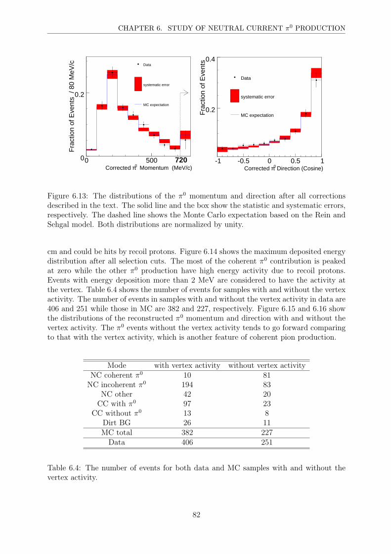
CHAPTER 6. STUDY OF NEUTRAL CURRENT π0 PRODUCTION
Momentum (MeV/c)0πCorrected 0 500
Fra
ctio
n of
Eve
nts
/ 80
MeV
/c
0
0.2
Data
systematic error
MC expectation
720 Direction (Cosine)0πCorrected
-1 -0.5 0 0.5 1
Fra
ctio
n of
Eve
nts
0.2
0.4
Data
systematic error
MC expectation
Figure 6.13: The distributions of the π0 momentum and direction after all correctionsdescribed in the text. The solid line and the box show the statistic and systematic errors,respectively. The dashed line shows the Monte Carlo expectation based on the Rein andSehgal model. Both distributions are normalized by unity.
cm and could be hits by recoil protons. Figure 6.14 shows the maximum deposited energydistribution after all selection cuts. The most of the coherent π0 contribution is peakedat zero while the other π0 production have high energy activity due to recoil protons.Events with energy deposition more than 2 MeV are considered to have the activity atthe vertex. Table 6.4 shows the number of events for samples with and without the vertexactivity. The number of events in samples with and without the vertex activity in data are406 and 251 while those in MC are 382 and 227, respectively. Figure 6.15 and 6.16 showthe distributions of the reconstructed π0 momentum and direction with and without thevertex activity. The π0 events without the vertex activity tends to go forward comparingto that with the vertex activity, which is another feature of coherent pion production.
Mode with vertex activity without vertex activityNC coherent π0 10 81
NC incoherent π0 194 83NC other 42 20
CC with π0 97 23CC without π0 13 8
Dirt BG 26 11MC total 382 227
Data 406 251
Table 6.4: The number of events for both data and MC samples with and without thevertex activity.
82
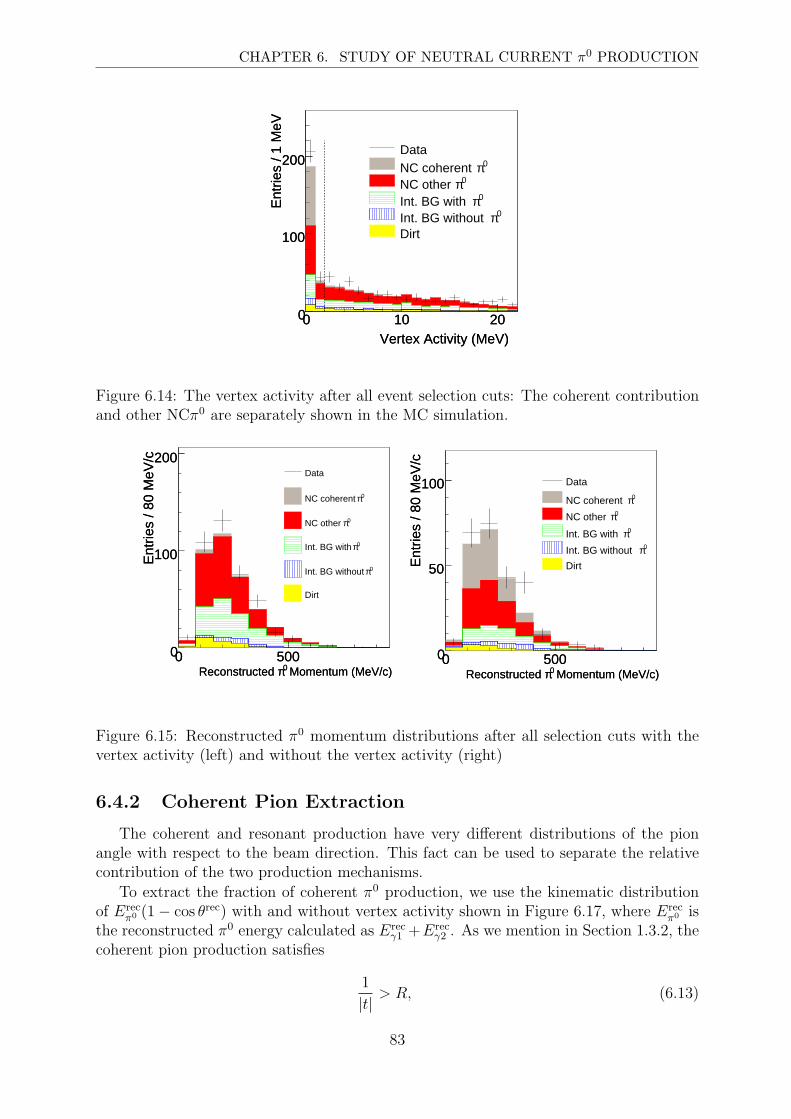
CHAPTER 6. STUDY OF NEUTRAL CURRENT π0 PRODUCTION
Vertex Activity (MeV)0 10 20
Ent
ries
/ 1 M
eV
0
100
200
Vertex Activity (MeV)0 10 20
Ent
ries
/ 1 M
eV
0
100
200Data
0πNC coherent 0πNC other
0πInt. BG with 0πInt. BG without
Dirt
Figure 6.14: The vertex activity after all event selection cuts: The coherent contributionand other NCπ0 are separately shown in the MC simulation.
Momentum (MeV/c)0πReconstructed 0 500
Ent
ries
/ 80
MeV
/c
0
100
200
Momentum (MeV/c)0πReconstructed 0 500
Ent
ries
/ 80
MeV
/c
0
100
200Data
0πNC coherent
0πNC other
0πInt. BG with
0πInt. BG without
Dirt
Momentum (MeV/c)0πReconstructed 0 500
Ent
ries
/ 80
MeV
/c
0
50
100
Momentum (MeV/c)0πReconstructed 0 500
Ent
ries
/ 80
MeV
/c
0
50
100 Data0πNC coherent
0πNC other 0πInt. BG with
0πInt. BG without
Dirt
Figure 6.15: Reconstructed π0 momentum distributions after all selection cuts with thevertex activity (left) and without the vertex activity (right)
6.4.2 Coherent Pion Extraction
The coherent and resonant production have very different distributions of the pionangle with respect to the beam direction. This fact can be used to separate the relativecontribution of the two production mechanisms.
To extract the fraction of coherent π0 production, we use the kinematic distributionof Erec
π0 (1 − cos θrec) with and without vertex activity shown in Figure 6.17, where Erecπ0 is
the reconstructed π0 energy calculated as Erecγ1 +Erec
γ2 . As we mention in Section 1.3.2, thecoherent pion production satisfies
1
|t|> R, (6.13)
83

CHAPTER 6. STUDY OF NEUTRAL CURRENT π0 PRODUCTION
direction (Cosine)0πReconstructed -1 0
Ent
ries
0
50
100
direction (Cosine)0πReconstructed -1 0
Ent
ries
0
50
100Data
0πNC coherent
0πNC other
0πInt. BG with
0πInt. BG without
Dirt
direction (Cosine)0πReconstructed -1 0
Ent
ries
0
50
direction (Cosine)0πReconstructed -1 0
Ent
ries
0
50
Data
0πNC coherent
0πNC other
0πInt. BG with
0πInt. BG without
Dirt
Figure 6.16: Reconstructed π0 direction distributions after all selection cuts with thevertex activity (left) and without the vertex activity (right)
where t and R are the four-momentum transfer to the target nucleus from the neutrinoand the radius of target nucleus, respectively. This means that the cross section decreaserapidly when 1/|t| become smaller than R. Then, the condition expressed as
1
t2> R2, (6.14)
is also satisfied for the coherent pion production. From Equation 6.14, one can deduce
Eπ0(1 − cos θπ0) <1
R(6.15)
as described in [99]. Here, the Eπ0 and θπ0 are the energy and direction of the emitted π0,respectively. This is why the Erec
π0 (1− cos θrec) is a good valuable to separate the coherentπ0 contribution from the resonant π0 production as well as t. We fit two Erec
π0 (1− cos θrec)distributions with and without the vertex activity by using three templates made bydividing the final MC sample into NC coherent π0, NC resonant π0 and backgroundsamples. Two parameters, Rcoh and Rres scale the NC coherent π0 and NC resonantπ0 templates independently. The background sample is fixed to the value of the MCprediction although the systematic errors on the background prediction are taken intoaccount. The expected number of events in the i-th bin in the Erec
π0 (1−cos θrec) distributionis expressed as:
N expi = Rcoh × N coh
i + Rres × N resi + NBG
i (6.16)
The fit minimizes the following χ2:
χ2 = −2 lnf(Nobs; N exp)
f(Nobs; Nobs), (6.17)
where Nobs(exp) represents the observed (expected) number of events in all bins
(Nobs(exp)1 , N
obs(exp)2 , . . ., N
obs(exp)N ) and f(Nobs; N exp) is the Poisson likelihood to find Nobs
84

CHAPTER 6. STUDY OF NEUTRAL CURRENT π0 PRODUCTION
) (MeV)0π recθ (1-cos 0π
recE
0 200 400
Ent
ries
/ 25
MeV
0
50
) (MeV)0π recθ (1-cos 0π
recE
0 200 400
Ent
ries
/ 25
MeV
0
50
Data
0πNC coherent
0πNC other
0πInt. BG with
0πInt. BG without
Dirt
) (MeV)0π recθ (1-cos 0π
recE0 200 400
Ent
ries
/ 25
MeV
0
50
) (MeV)0π recθ (1-cos 0π
recE0 200 400
Ent
ries
/ 25
MeV
0
50
Data
0πNC coherent
0πNC other
0πInt. BG with
0πInt. BG without
Dirt
Figure 6.17: The Erecπ0 (1 − cos θrec) distributions before fitting with (left) and without
(right) vertex activity
events when N exp events are expected. When the systematic errors for each bin and theircorrelation expressed with covariance matrix Vjk (j, k = 1, 2, . . . , N(= 39)) are given, thelikelihood is expressed as
f(Nobs; N exp; V ) = A
∫ [[ N∏i=1
dxixi
Nobsi e−xi
Nobsi !
]× exp
[−1
2
N∑j=1
N∑k=1
(xj − N expj )V −1
jk (xk − N expk )
]], (6.18)
where A is the normalizing constant. To calculate this integral, we generate 1000 MCexpectations with random variations drawn within the systematic uncertainties for eachbin. All systematic sources described in Section 6.2.4 are taken into account. Using xi,m
for the m-th expectation in the i-th bin, the likelihood is expressed as :
f(Nobs; N exp; V ) =1
M
∑m
∏i
xNobs
ii,m e−xi,m
Nobsi
, (6.19)
where M is the total number of random samples (1000). The result of the fit is:
Rcoh = 0.97 ± 0.19, (6.20)
Rres = 1.25 ± 0.13. (6.21)
The Erecπ0 (1− cos θrec) distribution after the fitting is shown in Figure 6.19. The χ2 per
degree of freedom (DOF), before the fit is 31.5/39 = 0.81, and it is 26.5/37 = 0.71 afterthe fit. Figure 6.18 shows three contours corresponding to one, two and three standarddeviations from the best fit point. The statistic error and all systematic errors are includedin the errors of Rcoh and Rres. Without the systematic errors, we obtain 0.98± 0.18(stat.)
85

CHAPTER 6. STUDY OF NEUTRAL CURRENT π0 PRODUCTION
resR0 1 2
coh
R
0
1
2
1 sigma
2 sigma
3 sigma
Figure 6.18: The contours corresponding to one, two and three standard deviations fromthe best fit point
and 1.19 ± 0.10(stat.) for Rcoh and Rres, respectively. Hence, the uncertainty of themeasurement are dominated by the statistic uncertainty. The dominant systematic sourceis the detector response. Figure 6.20 and 6.21 show the distributions of the reconstructionπ0 momentum and direction with or without the vertex activity after fitting.
)0π recθ(1-cos 0π
recE0 200 400
Ent
ries
/ 25
MeV
0
50
)0π recθ(1-cos 0π
recE0 200 400
Ent
ries
/ 25
MeV
0
50
Data
0πNC coherent
0πNC other
0πInt. BG with
0πInt. BG without
Dirt
)0π recθ(1-cos 0π
recE
0 200 400
Ent
ries
/ 25
MeV
0
50
)0π recθ(1-cos 0π
recE
0 200 400
Ent
ries
/ 25
MeV
0
50
Data
0πNC coherent
0πNC other
0πInt. BG with
0πInt. BG without
Dirt
Figure 6.19: The Erecπ0 (1−cos θrec) distributions after fitting with (left) and without (right)
vertex activity
The ratio of the NC coherent π0 production to the total CC cross sections from theMC prediction based on the Rein and Sehgal model is 1.21 × 10⁻². Hence, the cross
86

CHAPTER 6. STUDY OF NEUTRAL CURRENT π0 PRODUCTION
Momentum (MeV/c)0πReconstructed 0 500
Ent
ries
/ 80
MeV
/c
0
100
200
Momentum (MeV/c)0πReconstructed 0 500
Ent
ries
/ 80
MeV
/c
0
100
200Data
0πNC coherent
0πNC other
0πInt. BG with
0πInt. BG without
Dirt
Momentum (MeV/c)0πReconstructed 0 500
Ent
ries
/ 80
MeV
0
50
100
Momentum (MeV/c)0πReconstructed 0 500
Ent
ries
/ 80
MeV
0
50
100 Data
0πNC coherent
0πNC other
0πInt. BG with
0πInt. BG without
Dirt
Figure 6.20: Reconstructed π0 momentum distributions after fitting with the vertex ac-tivity (left) and without vertex activity (right)
Direction (Cosine)0πReconstructed -1 0
Ent
ries
0
50
100
Direction (Cosine)0πReconstructed -1 0
Ent
ries
0
50
100Data
0πNC coherent
0πNC other
0πInt. BG with
0πInt. BG without
Dirt
Direction (Cosine)0πReconstructed -1 0
Ent
ries
0
50
Direction (Cosine)0πReconstructed -1 0
Ent
ries
0
50
Data
0πNC coherent
0πNC other
0πInt. BG with
0πInt. BG without
Dirt
Figure 6.21: Reconstructed π0 direction distributions after fitting with the vertex activity(left) and without vertex activity (right)
section ratios are measured to be:
σ(NCcohπ0)
σ(CC)= Rcoh ×
σ(NCcohπ0)MC
σ(CC)MC
= Rcoh × 1.21 × 10−2
= (1.17 ± 0.23) × 10−2, (6.22)
where Rcoh is 0.97±0.19. The mean neutrino energy for NC coherent π0 events in thesample is estimated to be 1.0 GeV. This result is 5.8 standard deviations above the nocoherent production assumption. The measured cross section is also consistent with theMC prediction based on the Rein and Sehgal model [32]. The result is an evidence of
87

CHAPTER 6. STUDY OF NEUTRAL CURRENT π0 PRODUCTION
non-zero coherent pion production via neutral current interaction at the mean neutrinoenergy of 1.0 GeV.
6.5 Summary
The ratio of the NCπ0 production to total CC cross sections is measured to be [7.7±0.5(stat.)± 0.5(sys.)]× 10−2 at mean neutrino energy 1.1 GeV. The MC prediction basedon the Rein and Sehgal model [18] is 6.8 × 10⁻². We achieve less than 10 % uncertaintywhich is required for the νµ → νe oscillation measurement down to the sensitivity ofsin2 2θ13 ∼ 10−2.
The measured shapes of the π0 momentum and angular distributions, as shown inFigure 6.12, agree with the MC predictions within uncertainties. This means that theintra-nuclear interaction models implemented in NEUT well describe the kinematics ofNCπ0 production within the measured error (∼10 %).
The cross section ratio of NC coherent π0 production to the total CC interaction ismeasured to be (1.17 ± 0.23 ) × 10−2 based on the Rein and Sehgal model [32], whilethe MC prediction is 1.21 × 10⁻². This result is an evidence of non-zero coherent pionproduction via neutral current interaction at the mean neutrino energy of 1.0 GeV.
6.6 Discussion
We achieve three goals mentioned at the beginning: the measurement of the NCπ0
cross section ratio, the π0 kinematics distribution and the coherent π0 contribution.In this session, first, we discuss the impact of our results on the neutrino physics and
the future prospects for each topic. Then, we discuss the possibility of increasing theNCπ0 detection efficiency in future experiments.
6.6.1 Impact of our Results on Neutrino Physics and FutureProspects
NCπ0 Cross Section
We achieve less than 10 % uncertainty for the NCπ0 cross section ratio (σ(NCπ0)/σ(CC))so that we can predict the NCπ0 background events precise enough for the νµ → νe oscil-lation search at the sensitivity of sin2 2θ13 down to 10−2.
However, this is just requirement for the T2K phase I. If νµ → νe is not observed insin2 2θ13 ≥ 10−2, a further νµ → νe search down to sin2 2θ13 ∼ 10−3 may be conductedin the T2K phase II with the upgraded accelerator and Hyper-Kamiokande [14]. In thiscase, the 5 % uncertainty for the NCπ0 cross section is required to obtain the sensitivity ofsin2 2θ13 ∼ 10−3 [14]. For more precise measurements, at least, the statistical uncertaintyshould be decreased by increasing the detection efficiency as described in Section 6.6.2
After we find the νµ → νe mode, we will search for the CP violation (CP phase δ, asshown in Equation 1.2). To extract the CP phase, we compare the probability of νµ → νe
transition to that of νµ → νe transition. Therefore, we have to perform the measurementof νµ → νe. This requires that the NCπ0 production by antineutrinos should be measuredwith the similar uncertainty to NCπ0 by neutrinos. We also took antineutrino data in
88

CHAPTER 6. STUDY OF NEUTRAL CURRENT π0 PRODUCTION
the SciBooNE experiment. The analysis described in this chapter could be applied to theantineutrino data except that we need subtract the 30 % contamination of neutrinos.
π0 Kinematics
Validation of the nuclear model is important because we have to rely on the nuclearmodel to predict the NCπ0 cross section with different nuclear targets. For example, weneed to predict the NCπ0 cross section on water for T2K, which is using a water Cherenkovdetector as the far detector.
As described in Section 6.3.5, the good data/MC agreement of the π0 momentum andangular distributions confirms that the intra-nuclear interaction models implemented inNEUT well describe the kinematics of NCπ0 production within the measured error (∼10%). Hence we have a confidence in the nuclear model in NEUT.
However, the nuclear model in NEUT will be not enough to predict the more precisecross section in future. In this case, we need direct measurements with given nucleartargets. For T2K, the measurement with a water target at the neutrino energy below 1GeV is desired and plan. To obtain the cross section with various nuclear targets (carbon,iron and lead), the MINERνA experiment is now under construction [100].
Coherent Pion Production
Although our measurement of the cross section of NC coherent π0 production is consis-tent with the prediction by the Rein and Sehgal model, there are still unresolved questions.
As we describe in Section 4.2.1, the model predicts the relation between the neutral andcharged current coherent pion production cross sections as σ(CC) = 2×σ(NC). However,SciBooNE [49] reports no observation of CC coherent pion at the neutrino energy rangeof 1-2 GeV. Hence, the Rein and Sehgal model does not reproduce the SciBooNE data inthis sense. In addition, the MiniBooNE also observed NC coherent pion production, butwhich is 65 % of the Rein and Sehgal prediction, at mean neutrino energy of 1.2 GeV [29].So far our NC coherent π0 measurement is also consistent with the MiniBooNE resultwithin our statistical error. We need to increase the statistics to compare our result withMiniBooNE. This may be possible in future experiments as described in Section 6.6.2.
From these facts, the study of coherent pion production is still on going in SciBooNE.For the CC coherent pion production, we found the data excess comparing to the zerocoherent pion prediction in the forward pion sample (θπ < 35) both for neutrino andantineutrino data [101,102]. The short summary of these recent study of the CC coherentpion is described in Appendix D. Also for the NC coherent π0 production, the detailstudy of the kinematics of the emitted π0 is desired. This is also possible by increasingthe statistics as described in Section 6.6.2.
6.6.2 Increasing the Detection Efficiency
As described above, more precise measurements will be desired in future. In this thesis,for the coherent π0 fraction, the statistic uncertainty is dominant. For the cross sectionratio (σ(NCπ0)/σ(CC)) measurement, the statistic uncertainty is equal to the systematicuncertainty. Hence, increasing the statistics significantly reduces the uncertainties of ourmeasurements.
89

CHAPTER 6. STUDY OF NEUTRAL CURRENT π0 PRODUCTION
However, as described in Section 5.5.12, the detection efficiency of NCπ0 is 5.3 %, whichis small. In this section, we discuss the possibilities of increasing the detection efficiencyto reduce the statistical uncertainties. The main reason of the low detection efficiency issmall gamma conversion probability of SciBar. The second reason is mis-identification ofgamma rays.
Gamma Conversion Probability
The main reason of the small detection efficiency is the small probability of gammaconversion in SciBar. Since the length of SciBar in the beam direction is four radiationlengths, a significant fraction of gamma rays escape from SciBar without conversion. In30% of events with a π0 emitted in the SciBar fiducial volume, both gamma rays convertin SciBar; in 38%, only one gamma ray converts in SciBar; in 32%, neither gamma rayconverts in SciBar. Since we aim to reconstruct two gamma rays to identify the NCπ0
events, the maximum detection efficiency attainable is 30 %. Figure 6.22 and 6.23 showthe conversion probability of two gamma rays from π0 as a function of the π0 kinematics(momentum and direction) and vertices. The probability goes down for the π0 producedaround the edge of SciBar as expected while much less dependence of the π0 kinematicsexists. To increase the gamma conversion probability, we need a detector with longerradiation length. To obtain the longer radiation length, the T2K experiment develop adetector optimized for the π0 detection called “P0D” as one of the near detectors. Thebasic idea of P0D is inserting lead converters between scintillator planes.
momentum (MeV/c)0πTrue
0 500 1000
Pro
babi
lity
0
1
momentum (MeV/c)0πTrue
0 500 1000
Pro
babi
lity
0
1
convertsγ0
convertsγ1
convertγ2
direction (Cosine)0πTrue
-1 0 1
Pro
babi
lity
0
1
direction (Cosine)0πTrue
-1 0 1
Pro
babi
lity
0
1
convertsγ0
convertsγ1
convertγ2
Figure 6.22: The conversion probability of two gamma rays from π0 as a function of π0
momentum (left plot) and direction (right plot). The contribution from both gammarays conversion, one gamma ray conversion and no gamma ray conversion, are shownseparately.
Mis-identification of Gamma Ray
To select gamma rays, we reject the proton and muon candidate tracks. For example,the requirement of at least two extended tracks (Section 5.5.9) rejects about 140 NCπ0
signal events by identifying a gamma ray as a proton-like tracks. There are possibilities
90

CHAPTER 6. STUDY OF NEUTRAL CURRENT π0 PRODUCTION
vertex X (cm)0π -100 0 100
Pro
babi
lity
0
1
vertex X (cm)0π -100 0 100
Pro
babi
lity
0
1
convertsγ0
convertsγ1
convertγ2
vertex Y (cm)0π -100 0 100
Pro
babi
lity
0
1
vertex Y (cm)0π -100 0 100
Pro
babi
lity
0
1
convertsγ0
convertsγ1
convertγ2
vertex Z (cm)0π 0 100
Pro
babi
lity
0
1
vertex Z (cm)0π 0 100
Pro
babi
lity
0
1
convertsγ0
convertsγ1
convertγ2
Figure 6.23: The conversion probability of two gamma rays from π0 as a function of π0
vertex for each dimension (x, y, z from the left).
to distinguish gamma rays from proton-like tracks. One possible variable is track length.Figure 6.24 shows the track length of proton-like tracks rejected by the requirement of atleast two extended tracks. The track length of gamma rays tends to be shorter than thatof protons. Although using only the track length is still hard to distinguish gamma rays
0 50 1000
200
Length (cm)0 50 100
Ent
ries
0
200
Data
Gamma
Muon
Proton
Other
Figure 6.24: The track length of proton-like tracks rejected by requirement of at least twoextended tracks.
from protons, the combination with other valuables may make it possible. For example,protons deposit larger energy near the stopping point than at the beginning. On theother hand, the maximum energy deposit in gamma rays should be located around thecenter of whole track since the number of e−(e+) in the electromagnetic showers (gammarays) increases until their energies are not enough to produce another e+e− and decreasesafter that. Further study in this direction may enable us to distinguish gamma rays fromprotons.
In addition, the requirement of at least two extended tracks rejects about 90 NCπ0
signal events by identifying two back-to-back gamma rays as one gamma ray consisting oftwo co-linear tracks (one extended track). It may be possible to distinguish two back-to-back gamma rays from one gamma ray broken into to co-linear tracks by using the trackdirection. This is because the two back-to-back gamma rays have opposite directions whilethe two co-linear tracks made by a single gamma ray have same directions. The timing
91

CHAPTER 6. STUDY OF NEUTRAL CURRENT π0 PRODUCTION
difference between the track edges may be able to determine the track direction. Sincetypical gamma ray track length is roughly 30 cm corresponding to 1 ns transportationat speed of the light, the timing resolution better than 1 ns is desired. Using SciBar, weneed more precise timing calibration because the SciBar timing resolution evaluated withcosmic ray data is now 1.6 ns.
Since the current expected number of the NCπ0 signals and the detection efficiencyare 368 and 5.3 % after all event selections, respectively, the detection efficiency couldbe increased up to (90 + 140 + 368)/368 × 0.053 = 0.086 if the improvement describedabove is possible. Considering that we can increase the gamma conversion probability upto 100 % by inserting lead planes, the detection efficiency attainable in future is up to0.086 × (100/30) ∼ 30%.
92

Chapter 7
Conclusions
The SciBooNE experiment is designed for measuring neutrino-nucleus cross sectionsat the neutrino energy around 1 GeV. The measurement of the π0 production via NCinteraction is the primary motivation of the SciBooNE experiment. In this thesis, wepresent a study of NCπ0 production from muon neutrinos scattering on a polystyrene(C8H8) target in the SciBooNE experiments using SciBooNE’s full neutrino data set,corresponding to 0.99 × 10²⁰ protons on target.
Understanding the NCπ0 production at the neutrino energy of 1 GeV is essential for theneutrino oscillation experiments because the NCπ0 production is a dominant backgroundfor νµ → νe oscillation measurements. The νµ → νe oscillation is not yet discoveredand its corresponding mixing angle θ13 is constrained as sin2 2θ13 < 0.15 at the 90 %confidence level. The new neutrino oscillation experiments such as T2K and NOνA aimat the sensitivity of sin2 2θ13 below 10−2. To achieve this, the NCπ0 production must bemeasured within 10 % uncertainty. At the neutrino energy around 1 GeV, there are twomain π0 production mechanisms: resonant pion production and coherent pion production.Although several theoretical models exist to describe these π0 production mechanismsincluding the nuclear effects, there are discrepancies among these predictions. Hence,more experimental inputs are essential. However, the cross section of the neutral currentπ0 production was not measured within the 10 % uncertainty, especially in the neutrinoenergy below 1 GeV. Not only the total cross section but also the kinematic distribution ofthe emitted π0 must be measured. This is because the intra-nuclear interaction modifyingthe primary π0 via simple neutrino-nucleon scatterings is also poorly known.
The coherent pion production have drawn much attention also in the neutrino in-teraction physics. This is because the Rein and Sehgal model used widely in neutrinooscillation experiments can not explain recent experimental results such as K2K, Sci-BooNE and MiniBooNE at the mean neutrino energy around 1 GeV. Especially, the K2Kand SciBooNE experiment report null observation of the CC coherent pion production.Hence, it is important to measure the NC coherent pion production.
We have measured the cross section ratio of the NCπ0 production to the total CCinteraction and the π0 kinematic distribution such as momentum and direction. For thecross section ratio, we obtain
σ(NCπ0)
σ(CC)= (7.7 ± 0.5(stat.) ± 0.5(sys.)) × 10−2.
The mean energy of neutrinos producing detected π0s is 1.1 GeV. The MC prediction
93

CHAPTER 7. CONCLUSIONS
with the Rein-Sehgal model implemented in our neutrino interaction simulation programwith nuclear effects is 6.8 × 10⁻². Therefore, our result agrees with the MC prediction.We achieve less than 10 % uncertainty which is required for the νµ → νe oscillationmeasurement down to the sensitivity of sin2 2θ13 ∼ 10−2.
The measured shapes of the π0 momentum and angular distributions, as shown inFig. 6.12 agree with the MC prediction. This means that the intra-nuclear interactionmodels describe our data with our uncertainty level (∼10 %).
We also measure the cross section ratio of the NC coherent pion production to thetotal CC interactions. We obtain
σ(NCcoherentπ0)
σ(CC)= (1.17 ± 0.23) × 10−2.
The mean energy of neutrinos producing detected coherent π0s is 1.0 GeV. This result is5.8 standard deviations above the no coherent production assumption. This cross sectionratio is consistent with the prediction by the Rein and Sehgal model, which is 1.21×10⁻².The Rein and Sehgal model also predicts the relation between the CC and NC coherentpion production: σ(CC) = 2× σ(NC). However, SciBooNE reports no observation of theCC coherent pion production. Hence, the Rein and Sehgal model can not explain bothNC and CC coherent pion result of SciBooNE. This creates active controversies on themodel of coherent pion production, and understanding of coherent pion production is inprogress.
94

Appendix A
The Gamma and π0 Reconstruction
In this chapter, the details of γ and π0 reconstruction are described. First, we describethe method of the γ reconstruction; extended track and SciBar-EC matching. Then, wedescribe the performance of the γ and π0 reconstruction including angular resolution,momentum resolution and so on.
A.1 Extended Track
In order to improve the reconstruction of γs , we developed the new reconstructionalgorithm called extended track. Extended tracks are reconstructed based on the tracks.Since extended tracks are used after the EC cut, the event sample used for plots in thissection is after the EC cut described in Section 5.5.8.
A.1.1 Track Merge
Some of single γs are broken into two tracks in SciBar (Figure A.1).We should re-construct such events as a single γ events by merging tracks on a common straight line.To do this, we fit hits associated to two tracks in each view with a straight line and wemerge them if both reduced χ2s are less than 50. Figure A.2 shows the distribution ofthe reduced χ2. The red color shows the case where two tracks are made by same particle(correct pairing), while the blue color shows the case where two tracks are made by differ-ent particle (wrong pairing). The 2D plots between the reduced χ2s of top view and sideview are shown in Figure A.3. After all event selections, about 7 % of selected extendedtracks are made by merged tracks.
A.1.2 Energy Reconstruction
After merging tracks, hits around the merged tracks are collected for energy recon-struction. The region where hits are collected is illustrated in Figure A.4. The energy ofmerged tracks are calculated as a sum of energy deposit in this region. We consider twovariables to decide the size of this region (R in Figure A.4). One is “energy collectionefficiency” (εγ) and the other “gamma energy purity” (Pγ). These two variable are definedas
εγ =gamma energy in extended track
true gamma energy(A.1)
95

APPENDIX A. THE GAMMA AND π0 RECONSTRUCTION
Figure A.1: An example for 2γs from π0. Red dots show hits in SciBar and colored lineshows tracks. One γ is broken into two tracks in this events
(Top View)2χReduced 0 100 200
Ent
ries
0
200
(Top View)2χReduced 0 100 200
Ent
ries
0
200
correct paring
wrong pairing
(Side View)2χReduced 0 100 200
Ent
ries
0
200
(Side View)2χReduced 0 100 200
Ent
ries
0
200
correct paring
wrong pairing
Figure A.2: Distribution of reduced χ2 by fitting hits in two tracks for both view. The leftplot shows top view and the right shows side view. The red color shows correct pairing,while the blue color shows wrong pairing
(Top View)2χReduced
0 100 200
(S
ide
Vie
w)
2 χR
educ
ed
0
100
200
0
100
200
300
400
500
600
700
(Top View)2χReduced
0 100 200
(S
ide
Vie
w)
2 χR
educ
ed
0
100
200
0
10
20
30
40
50
Figure A.3: 2D distribution of reduced χ2 by fitting hits in two tracks for both view in theMC simulation. The left plot shows correct pairing and the right shows wrong pairing.
96

APPENDIX A. THE GAMMA AND π0 RECONSTRUCTION
Pγ =gamma energy in extended track
total energy in extended track(A.2)
The εγ become large with large R because we collect γ hits even far from tracks. But the
R = 20 cm R = 20 cm
The 2D projection of a 3D track
Hit collection rejion
Figure A.4: Hit collection region. Hits are collected in this region for both view
Pγ becomes small with large R because we collect hits associated with different particlesnear the γ ray. Figure A.5 shows εγ and Pγ dependence of “R”. Since the εγ begins tosaturate around R = 20 cm but the Pγ decreases linearly up to R = 30 cm, the R = 20 cmis chosen. The performance of the energy reconstruction will be discussed in Section A.3.
R (cm)0 20
Effi
cien
cy a
nd P
urity
0.6
0.8
1
Figure A.5: Pγ(filled circle) and εγ(empty circle) as a function of R shown in Figure A.4
97

APPENDIX A. THE GAMMA AND π0 RECONSTRUCTION
A.1.3 Direction Reconstruction
The reconstructed γ direction is used for the π0 vertex reconstruction, which is animportant quantity in this analysis. Figure A.6 shows the number of hits around tracksfor each R region without hits associated with tracks. (0cm < R < 5cm, 5cm < R <10cm, 10cm < R < 15cm, 15cm < R < 20cm). The discrepancy between data and MCsimulation become large for the large R. Therefore, we only use information of tracks forthe angle reconstruction, which means that hits newly associated in the way described inSection A.1.2 are not used for the direction reconstruction.
NHits0 5 10
Ent
ries
0
1000
NHits0 5 10
Ent
ries
0
1000
gamma
other
0 cm < R < 5 cm
NHits0 5 10
Ent
ries
0
1000
NHits0 5 10
Ent
ries
0
1000
gamma
other
5 cm < R < 10 cm
NHits0 5 10
Ent
ries
0
1000
NHits0 5 10
Ent
ries
0
1000
gamma
other
10 cm < R < 15 cm
NHits0 5 10
Ent
ries
0
1000
NHits0 5 10
Ent
ries
0
1000
gamma
other
15 cm < R < 20 cm
Figure A.6: The red (blue) histogram shows the distribution of the number of hitsaround gamma rays (other particles) for each R region (0cm < R < 5cm, 5cm < R <10cm, 10cm < R < 15cm, 15cm < R < 20cm).
98

APPENDIX A. THE GAMMA AND π0 RECONSTRUCTION
A.2 SciBar-EC Matching
Some of γs observed in SciBar have energy deposit in EC. After the event reconstruc-tion in SciBar we search for EC clusters pointed by tracks from SciBar. Since we use ECinformation at the EC cut, the sample used for plots shown in this section is before theEC cut. The procedure of finding matched EC cluster is described below.
1. Extrapolate a track for both view and getting x position at z = 178.4 (EC upstreamplane) ant y position at z = 184.61 cm (EC downstream).
2. Take EC clusters within 10 cm from x,y which are obtained above as a matched ECcluster (Figure A.7).
3. Repeat the procedure for all tracks.
Figure A.7 shows the distance between the extrapolated position and EC cluster positionfor gamma rays by the MC simulation and Figure A.8 are same plots for muons. The solidhistogram shows the case of correct matching where EC cluster and SciBar track comefrom the same particle, while the dashed histogram shows the case of wrong matchingwhere EC cluster and SciBar track made by different particle. There are peaks even forwrong matching of muons. This is the case that actual muon tracks are regarded as otherparticles by the algorithm matching reconstructed tracks and true particles. Matchingreconstructed tracks and true particles is sometimes difficult due to high track multiplicityor overlapped tracks. Since the EC cut is for rejecting muon rather than selecting γs,we regard the EC cluster within 10 cm from the extrapolated position as a matched ECcluster. After all event selections, about 17 % of selected extended tracks have matchedEC clusters.
(cm)EC-XextrapolateX-50 0 50
Arb
itrar
y U
nit
Correct Pairing
Wrong Pairing
(cm)EC-YextrapolateY-50 0 50
Arb
itrar
y U
nit
Correct Pairing
Wrong Pairing
Figure A.7: The distance between the extrapolated position and EC cluster position forgamma rays in the MC simulation. The left plots shows the upstream cluster and theright shows the downstream. (Solid line:correct matching, Dashed line:wrong matching)
A.3 Performance of Gamma Reconstruction
Here we discuss the performance of γ reconstruction. All plots in this section is after“π0mass cut”
99

APPENDIX A. THE GAMMA AND π0 RECONSTRUCTION
(cm)EC-XextrapolateX-50 0 50
Arb
itrar
y U
nit
Correct Pairing
Wrong Pairing
(cm)EC-YextrapolateY-50 0 50
Arb
itrar
y U
nit
Correct Pairing
Wrong Pairing
Figure A.8: The distance between the extrapolated position and EC cluster position formuons by the MC simulation. The left plots shows the upstream cluster and the rightshows the downstream. (Solid line:correct matching, Dashed line:wrong matching)
A.3.1 Gamma Angular Resolution
Figure A.9 shows angles between the reconstructed γ direction and the true γ direction.The sigma by guassian fitting of the distribution is about 6 degree while RMS is about14 degree. This difference comes from the long tail due to mis-reconstruction of γs.
Entries 113582
Mean 0.04558
RMS 13.7
/ ndf 2χ 74.4 / 7
Prob 1.898e-13
Constant 1.302e-10
Mean -0.2952
Sigma 5.536
(Degree)trueθ - recθ-90 -30 30 90
Arb
itrar
y U
nit
Entries 113582
Mean 0.04558
RMS 13.7
/ ndf 2χ 74.4 / 7
Prob 1.898e-13
Constant 1.302e-10
Mean -0.2952
Sigma 5.536
Figure A.9: The angles between reconstructed γ direction and true γ direction.
A.3.2 Gamma Energy Resolution
Figure A.10 shows the difference between reconstructed γ energy in extended trackand true energy deposit in SciBar. The sigma of the peak is 6.9 MeV and the mean of γenergy deposit in SciBar is 116 MeV in the MC simulation. The energy resolution of γ inSciBar is estimated to be 5.8 % at 116 MeV. There is a long tail in this distribution. This
100

APPENDIX A. THE GAMMA AND π0 RECONSTRUCTION
is due to mis-reconstruction. Figure A.11 shows the difference between the reconstructedenergy in the EC cluster and the true γ energy deposit in EC. The sigma of the peak is23 MeV and the mean of γ energy deposit in EC is estimated to be 72 MeV in the MCsimulation. Therefore the energy resolution of γ in EC is estimated to be 32 % at 72MeV.
Entries 113582
Mean -1.407
RMS 33.95
/ ndf 2χ 144 / 4
Prob 0
Constant 1.802e-10
Mean -2.795
Sigma 6.86
(MeV)true,SBγ - Erec,SB
γ E-200 0 200
Arb
itrar
y U
nit
Entries 113582
Mean -1.407
RMS 33.95
/ ndf 2χ 144 / 4
Prob 0
Constant 1.802e-10
Mean -2.795
Sigma 6.86
Figure A.10: The difference between thereconstructed energy in extended tracksand the true energy deposit by γ inSciBar.
Entries 15655
Mean -12.36
RMS 44.71
/ ndf 2χ 22.25 / 14
Prob 0.07372
Constant 9.054e-12
Mean -7.095
Sigma 23.48
(MeV)true,ECγ - Erec,EC
γ E-200 0 200
Arb
itrar
y U
nit
Entries 15655
Mean -12.36
RMS 44.71
/ ndf 2χ 22.25 / 14
Prob 0.07372
Constant 9.054e-12
Mean -7.095
Sigma 23.48
Figure A.11: The difference between thereconstructed energy in EC cluster andthe true energy deposit by γ in EC.
Not all gamma ray energy is deposited in, nor recorded by, the detector. Figure A.12shows the distribution of the actual energy collection efficiency defined as
Effact =gamma enengy in extended track
true gamma energy. (A.3)
Since the average of Effact is 76 %, the average lost energy is 24 %; 11% comes fromenergy loss in passive regions and gamma rays escaping from the detectors and 13 %comes from energy deposit in active regions but not assigned to the extended track. Thereconstructed energy could include energy deposited by other particles. Figure A.13 showsdistribution of the gamma purity defined as
Pγ =gamma energy in the extended track
all energy in the extended track. (A.4)
Since the average of the gamma purity is 85 %, 15% of the total energy in an extendedtrack comes from other particle on average. Due to this contamination, the effectiveenergy collection efficiency defined as:
Effeff =reconstructed energy of extended track
true gamma energy. (A.5)
is 85 % on average, which is larger than the average of Effact.Figure A.14 shows the distribution of the effective energy collection efficiency. Fig-
ure A.15 shows the 2D plot between the true gamma energy and the reconstructed energyof the extended track. The solid line on the plot shows the identity. The distribution isbelow the line since the effective energy collection efficiency is less than one.
101

APPENDIX A. THE GAMMA AND π0 RECONSTRUCTION
Entries 113582
Mean 0.7638
RMS 0.1524
Actual energy collection efficiency0 0.5 1
Arb
itary
Uni
t
Entries 113582
Mean 0.7638
RMS 0.1524
Figure A.12: Actual energy collection efficiency defined as gamma energy in extendedtrack divided by true gamma energy.
Entries 113582
Mean 0.8494
RMS 0.2001
purityγ0 0.5 1
Arb
itrar
y U
nit
Entries 113582
Mean 0.8494
RMS 0.2001
Figure A.13: Gamma purity defined as gamma energy in extended track divided byreconstructed energy of extended track.
102

APPENDIX A. THE GAMMA AND π0 RECONSTRUCTION
Entries 113582
Mean 0.8374
RMS 0.3082
Effective energy collection efficiency0 1 2
Arb
itrar
y U
nit
Entries 113582
Mean 0.8374
RMS 0.3082
Figure A.14: Effective energy collection efficiency defined as the reconstructed energy ofextended track divided by the true gamma energy.
Energy (MeV)γTrue 0 200 400
Ene
rgy
(MeV
)γ
Rec
onst
ruct
ed
0
200
400
0
0.1
0.2
0.3
0.4
0.5
0.6
0.7
0.8
0.9
1
Figure A.15: 2D plot between the true γ energy and the reconstructed energy of extendedtrack. The line shows identity.
103

APPENDIX A. THE GAMMA AND π0 RECONSTRUCTION
A.4 Performance of π0 Reconstruction
To check π0 reconstruction, we look at what kind of two particles are in the selectedpair of extended tracks in the NCπ0 mode after the π0 mass cut using the MC simulation.The result is shown in Table A.1. We use four types to categorize all the pairs. In the“correct 2γs” events, both γs from common π0 are correctly associated to two extendedtracks. In the “wrong 2γs” events, both extended tracks are associated to γs but thesetwo are coming from different π0s or just one single γ broken into isolated two extendedtracks. In the “1 γ + other” events, one extended track are associated to a γ but theother extended track is associated to other charged particle. In the “two other particles”events, both extended tracks are associated to other charged particles. Possible chargedparticles are protons,charged pions and muons. Among these four types, Only in first one“correct 2γs”, two extended tracks are correctly associated to π0 and the contaminationof this type is 87 % after the π0 mass cut. The plots shown in this section are using onlythe type “correct 2 γs” in the NCπ0 to see the π0 reconstruction performance.
pair type contamination (%)correct 2γs 87.3wrong 2γs 3.71γ + other 8.9
2 others particle 0.1
Table A.1: The type of the extended track pair after the π0 mass cut
A.4.1 π0 Vertex Resolution
Figure A.16 shows the difference of π0 vertex between the reconstructed vertex andthe MC true value after the π0 mass cut. The RMS is about 12 cm for all dimension.
A.4.2 π0 Angle Resolution
Figure A.17 shows the angle between the π0 reconstructed direction and the MC trueπ0 direction. RMS is about 15 degree and the sigma by gaussian fitting is about 6 degree.These values are close to the resolution of γ angle as we expected.
A.4.3 π0 Mass Resolution and Momentum Resolution
Figure A.18 shows the difference between the reconstructed π0 mass and MC true π0
mass (135 MeV/c2) before the π0 mass cut. The peak are negative because we do notcorrect the energy leakage of γs. The sigma by gaussian fitting is 28 MeV/c2 and the meanreconstructed mass is 119 MeV/c2. Therefore, the average reconstructed mass resolutionis about 23 %.
Figure A.19 shows the difference between the reconstructed π0 momentum and theMC true π0 momentum after the π0 mass cut. The peak are negative because of energyleakage of γs. The sigma by gaussian fitting is 37 MeV/c2 and the mean reconstructedmomentum is 223 MeV/c. Therefore, The average momentum resolution is about 17
104

APPENDIX A. THE GAMMA AND π0 RECONSTRUCTION
Entries 56791
Mean -0.1486
RMS 12.08
(cm)true - XrecX
-50 0 50
Arb
itrar
y U
nit
Entries 56791
Mean -0.1486
RMS 12.08
Entries 56791
Mean 0.04792
RMS 12.11
(cm)true - YrecY
-50 0 50
Arb
itrar
y U
nit
Entries 56791
Mean 0.04792
RMS 12.11
Entries 56791
Mean 0.7202
RMS 11.38
(cm)true - ZrecZ
-50 0 50
Arb
itrar
y U
nit
Entries 56791
Mean 0.7202
RMS 11.38
Figure A.16: The difference of π0 vertex between the reconstructed π0 vertex and thetrue value for each coordinates after the π0 mass cut. From the left, x,y and z verticesare shows, respectively.
Entries 56791
Mean -0.07074
RMS 14.99
/ ndf 2χ 85.6 / 8
Prob 3.622e-15
Constant 6.236e-11
Mean -0.6446
Sigma 5.557
(Degree)0π trueθ - 0π
recθ-90 -30 30 90
Arb
itrar
y U
nit
Entries 56791
Mean -0.07074
RMS 14.99
/ ndf 2χ 85.6 / 8
Prob 3.622e-15
Constant 6.236e-11
Mean -0.6446
Sigma 5.557
Figure A.17: The angle between the reconstructed π0 direction and the MC true π0
direction after the π0 mass cut
105

APPENDIX A. THE GAMMA AND π0 RECONSTRUCTION
Entries 65825
Mean -17.11
RMS 44.54
/ ndf 2χ 71.79 / 20
Prob 9.268e-08
Constant 3.141e-11
Mean -24.85
Sigma 27.57
)2 - 135 (MeV/cγ 2 recM
-200 0 200
Arb
itrar
y U
nit
Entries 65825
Mean -17.11
RMS 44.54
/ ndf 2χ 71.79 / 20
Prob 9.268e-08
Constant 3.141e-11
Mean -24.85
Sigma 27.57
Figure A.18: The difference between the reconstructed π0 mass and MC true π0 mass(135 MeV/c2) before the π0 mass cut
%. We already show the relation between the π0 true momentum and the reconstructedmomentum after the π0 mass cut in Figure 6.10. In the end, we put the summary tableof the π0 reconstruction performance in Table A.2.
Entries 56791
Mean -39.94
RMS 58.29
/ ndf 2χ 103.7 / 28
Prob 1.283e-10
Constant 1.879e-11
Mean -36.76
Sigma 36.81
(MeV/c)0π true - P0π
recP-200 0 200
Arb
itrar
y U
nit
Entries 56791
Mean -39.94
RMS 58.29
/ ndf 2χ 103.7 / 28
Prob 1.283e-10
Constant 1.879e-11
Mean -36.76
Sigma 36.81
Figure A.19: The difference between the reconstructed π0 momentum and the MC trueπ0 momentum after the π0 mass cut
106

APPENDIX A. THE GAMMA AND π0 RECONSTRUCTION
π0 angle resolution 6 degree (sigma)mean π0 reconstructed mass 119 MeV/c2
π0 mass resolution 23 % (sigma)mean π0 reconstructed momentum 223 MeV/c
π0 momentum resolution 17 % (sigma)
Table A.2: The performance the of π0 reconstruction
107

Appendix B
Neutrino Interaction In TheSurrounding Material
Neutrino interactions occur outside of the detector such as the wall of the detectorhall or dirt and produce secondary particles. The secondary particles by such interactionssometimes make hits in the SciBooNE detectors. We call these events “dirt backgroundevents”. For NC π0 measurement, neutrino induced π0 production outside of the detectorsuch as wall of the detector hall or dirt is a background. The estimate of the number ofdirt background events in the NC π0 sample by the MC simulation is important in thisanalysis.
B.1 Dirt material
We use concrete as material for both the wall and dirt in the MC simulation. Thecontamination of each element is shown in Tab. B.1 The density is 2.15 g/cm3. Thisestimation is very rough. Therefore we vary by ±20 % this density when we estimatesystematic uncertainty.
element contamination (%)H 1O 53Na 2Al 3Si 34K 1Ca 4Fe 1
Table B.1: The contamination of each element of our concrete
108

APPENDIX B. NEUTRINO INTERACTION IN THE SURROUNDING MATERIAL
B.2 The area of neutrino events
Figure B.1 shows the area where neutrino events are generated. For the neutrino crosssection, we use NEUT for C8H8, which is same for SciBar. About the coordination, X, yand z correspond to the horizontal, vertical and beam direction, respectively. The originof x and y is the center of SciBar and the origin of z is the upstream surface of SciBar.We generate neutrino events in the region, which is −5 m < x < 5 m, −5 m < y < 5 mand −5 m < z < 5 m for dirt MC simulation. Figure B.2 shows the vertex of neutrino
5 m
5 m
5 m
1.2 m
2.4 m
x (horizontal)
0.3m
z (beam axis)5 m5 m
5 m
5 m
z (beam axis)
y (vertical)
5 m
0.4 m
SciBar SciBarMRD MRD
TOP view Side view
The region where dirt events are generated
Figure B.1: The area where neutrino events are generated (green region)
interactions by the dirt MC simulation after all event selections. By Fig. B.2, the most ofneutrino interactions occur between ±2 m for all directions. Therefore, The region (±5 mfor x,y and z) is large enough.
X (cm)
-500 0 500
Arb
itrar
y U
nit
Y (cm)
-500 0 500
Arb
itrar
y U
nit
Z (cm)
-500 0 500
Arb
itrar
y U
nit
Figure B.2: The neutrino vertex of dirt MC after all event selections for NC π0
109

Appendix C
MC Expectation with SystematicUncertainty
Some of histograms are shown with systematic errors for each bin in this thesis. In thischapter, we describe how we calculate the size of systematic errors in such histograms.
To include the systematic uncertainty, we generate 1000 expectations within system-atic uncertainty and look at the variation of the value which we want to measure. Forsimplicity, we consider the case that we measure two value (N1, N2) with two independentsystematic source tagged as A,B. Since we have two sets of the systematic variationstagged as +,− (for example, MC sets with larger and smaller cross talk). we can get
NA+1 , NA−
1 , NB+1 , NB−
1
and
NA+2 , NA−
2 , NB+2 , NB−
2
for N1 and N2 (nominal MC expectations), respectively. Using them we define
σA+1 = NA+
1 − N1
σA−1 = NA−
1 − N1
σB+1 = NB+
1 − N1
σB−1 = NB−
1 − N1
σA+2 = NA+
2 − N2
σA−2 = NA−
2 − N2
σB+2 = NB+
2 − N2
σB−2 = NB−
2 − N2.
Then, we generate random numbers of ∆A1,i, ∆B
1,i, ∆A2,i and ∆B
2,i for i-th generation (0 <i < 1000). To obtain ∆A
1,i and ∆A2,i, we get xi using a gaussian random number generator
( Mean = 0, RMS = 1 ).If we get xi > 0
∆A1,i = σA+
1 ×xi (C.1)
∆A2,i = σA+
2 ×xi (C.2)
110

APPENDIX C. MC EXPECTATION WITH SYSTEMATIC UNCERTAINTY
otherwise,
∆A1,i = σA−
1 ×xi (C.3)
∆A2,i = σA−
2 ×xi. (C.4)
To obtain RB1,i and RB
2,i, we get yi using a gaussian random number generator ( Mean =0, RMS = 1 ). The yi must be obtained by the different random number generation forxi since the systematic sources of A and B are independent from each other. If we getyi > 0
∆B1,i = σB+
1 ×yi (C.5)
∆B2,i = σB+
2 ×yi (C.6)
otherwise,
∆B1,i = σB−
1 ×yi (C.7)
∆B2,i = σB−
2 ×yi. (C.8)
Finally we obtain i-the expectation for N1 and N2 expressed as
N1,i = N1 + ∆A1,i + ∆B
1,i (C.9)
N2,i = N2 + ∆A2,i + ∆B
2,i, (C.10)
respectively. When we obtain the RMS of F (N1, N2) (some function of N1 and N2), wecalculate
∆F (N1, N2) =
√√√√ 1
1000
1000∑i=1
(F (N1,i, N2,i) − F (N1, N2))2 (C.11)
respectively. We use ∆F (N1, N2) as the size of systematic error box.
111

Appendix D
Charged Current Coherent PionProduction
The SciBooNE collaboration reports no observation of CC coherent pion produc-tion [49]. However, as described in Section 6.6.1, further study reveals the data excesscomparing to the zero coherent pion prediction in the forward pion sample (θπ < 35) bothfor neutrino and antineutrino data. In this chapter, we present the summary of recentstudy of CC coherent pion production [101, 102]. For analyses presented in this chapter,NEUT is used for the neutrino interaction simulation. Hence, the Rein and Sehgal modelis employed for the coherent pion production.
D.1 Event Selection of CC Coherent Pion Produc-
tion
The same event selection cuts are applied for neutrino and antineutrino CC coherentpion search. Although the MC tuning is performed in the neutrino mode, it is not yetdone in the antineutrino mode.
We use the MRD-stopped event sample described in Section 5.4 as the CC eventsample. After the CC selection, we select events with one additional track originatingfrom the common vertex of the SciBar-MRD matched track. This additional track isrequired to be a pion-like track which means MuCL > 0.05 (Muon Confidence Level,Section 5.3.3). The recoil proton in the incoherent pion production can be identified byusing the energy deposit around the vertex (vertex activity). The CC coherent pion eventsdo not have the vertex activity. We also reduce the CC quasi-elastic events by using theangle (∆θp) between the expected proton track and the observed second track directions.In case of CC quasi-elastic events, the proton angle can be predicted by the muon angleand momentum, so that we expect ∆θp ∼ 0. In case of non-elastic events such as the pionproduction, we expect ∆θp 6= 0. Finally, we select events with the pion track candidatedirected forward, which is also the characteristic of coherent pion production. The detailsof the event selection cuts are described in [49,56].
112

APPENDIX D. CHARGED CURRENT COHERENT PION PRODUCTION
D.2 Study of CC Coherent Pion Production for Neu-
trino and Antineutrino
D.2.1 νµ CC Coherent Pion Production
2 (GeV/c)2Q0 0.1 0.2 0.3 0.4 0.5
2E
ntr
ies
/ 0.0
25 (
GeV
/c)
0
50
100
150
0 0.1 0.2 0.3 0.4 0.50
50
100
150
DATA
π CC coherent
π CC resonant
Other
CC QE
2 (GeV/c)2Q0 0.1 0.2 0.3 0.4 0.5
2E
ntr
ies
/ 0.0
25 (
GeV
/c)
0
10
20
30
40
0 0.1 0.2 0.3 0.4 0.50
10
20
30
40
DATA
π CC coherent
π CC resonant
Other
CC QE
Figure D.1: The Q2rec distribution for the MRD stopped CC coherent pion sample (left),
and the MRD penetrated CC coherent pion sample (right).
Figure D.1 (left) shows the Q2rec distribution for the selected events. The Q2
rec is calleda reconstructed Q2 calculated as
Q2rec = 2Erec
ν (Eµ − pµ cos θµ) − m2µ (D.1)
where Erecν is the reconstructed neutrino energy calculated by assuming CC quasi-elastic
kinematics,
Erecν =
1
2
(M2p − m2
µ) − (Mn − V )2 + 2Eµ(Mn − V )
(Mn − V ) − Eµ + pµ cos θµ
(D.2)
where Mp and Mn are the mass of proton and neutron, respectively, and V is the nuclearpotential, which is set to 27 MeV. In the signal region with Q2
rec less than 0.1 GeV/c2, 247CC coherent pion candidate events are observed, while the expected number of backgroundevents is 228±12. The selection efficiency for the signal is estimated to be 10.4%. Themean neutrino beam energy for true CC coherent pion events in the sample is estimatedto be 1.1 GeV after accounting for the effects of the selection efficiency.
We also use the MRD penetrated sample to search for CC coherent pion productionat higher energy. Events with the SciBar-MRD matched track not stopping in MRD butexiting from the downstream end of MRD are defined as the MRD penetrated sample.The same selection cuts are applied to the MRD penetrated sample to search for CCcoherent pion candidate events. Figure D.1 (right) shows the Q2
rec distribution for theMRD penetrated CC coherent pion sample. In the signal region, 57 CC coherent pioncandidates are observed, while the expected number of background events is 40±2.2. Theselection efficiency for the signal is estimated to be 3.1%. The mean neutrino beam energyfor true CC coherent pion events in the sample is estimated to be 2.2 GeV.
Since the data excess to the background level is small for both samples, we set 90 %confidence level upper limit on the cross section ratio of the CC coherent pion production
113

APPENDIX D. CHARGED CURRENT COHERENT PION PRODUCTION
to the total CC interaction at 0.67 × 10⁻² for a mean neutrino energy of 1.1 GeV and1.36×10−2 for that of 2.2 GeV. These limits correspond to 33 % and 67 % of the predictionby the Rein and Sehgal model at 1.1 GeV and 2.2 GeV, respectively. These limits arepublished in [49]. (GeV/c)µP
0 0.5 1 1.5
En
trie
s
0
20
40
60
80
0 0.5 1 1.50
20
40
60
80 DATA
π CC coherent ν
π CC resonant ν
BGν
NCν
CC otherν
CC QEν
µP
(degrees)µ
θ0 20 40 60 80
En
trie
s
0
50
100
0 20 40 60 800
50
100 DATA
π CC coherent ν
π CC resonant ν
BGν
NCν
CC otherν
CC QEν
µθ
(cm)πL0 50 100 150
En
trie
s
0
20
40
60
80
πL
0 50 100 1500
20
40
60
80 DATA
π CC coherent ν
π CC resonant ν
BGν
NCν
CC otherν
CC QEν
πL
(degrees)πθ0 50 100 150
En
trie
s
0
50
100
πθ
0 50 100 1500
50
100
DATA
π CC coherent ν
π CC resonant ν
BGν
NCν
CC otherν
CC QEν
πθ
Figure D.2: The pion angular distribution in CC coherent pion sample.
After we published the upper limits, further study is performed. Figure D.2 shows thedistribution of the pion angle with respect to the beam axis (θπ) for the MRD stoppedcoherent sample. There are data excess with respect to the background prediction at smallpion scattered angle. Motivated by this fact, both samples for neutrino and antineutrinois further divided into two sub-samples based on θπ: θπ < 30 and θπ > 30. In the case ofCC coherent pion production, muon and pion are expected to be emitted back-to-back inthe x-y plane because of the conservation of momentum. Therefore, the kinematic variablecalled ∆φ is defined as shown in Figure D.3. The coherent pion events are expected todistribute around ∆φ = 0. Figure D.4 shows ∆φ distributions in each sub-sample for
ν µ
π∆φ
X-Y plane
Figure D.3: Definition of the kinematic variable ∆φ.
114

APPENDIX D. CHARGED CURRENT COHERENT PION PRODUCTION
! µ
"#$
X-Y plane
FIGURE 5. Definition of the kinematic variable !" .
(degrees)!"-100 0 100
En
trie
s
0
10
20
30
40
<35 degrees)#
$ (!"
-100 0 1000
10
20
30
40 DATA
# CC coherent %
# CC resonant %
BG%
NC%
CC other%
CC QE%
<35 degrees)#
$ (!"
(degrees)!"-100 0 100
En
trie
s
0
10
20
30
40
>35 degrees)#
$ (!"
-100 0 1000
10
20
30
40 DATA
# CC coherent %
# CC resonant %
BG%
NC%
CC other%
CC QE%
>35 degrees)#
$ (!"
FIGURE 6. !" distributions for two different pion scattered angle regions in the MRD stopped coherent pion sample.
GeV and 2.2 GeV, respectively.
ACKNOWLEDGMENTS
The SciBooNE Collaboration gratefully acknowledge support from various grants, contracts and fellowships from the
MEXT (Japan), the INFN (Italy), the Ministry of Education and Science and CSIC (Spain), the STFC (UK), and the
DOE and NSF (USA). The author is grateful to the Japan Society for the Promotion of Science for support.
REFERENCES
1. D. Rein and L. M. Sehgal, Nucl. Phys. B 223, 29 (1983).2. M. Hasegawa et al. [K2K Collaboration], Phys. Rev. Lett. 95, 252301 (2005) [arXiv:hep-ex/0506008].3. A. A. Aguilar-Arevalo et al. [MiniBooNE Collaboration], Phys. Lett. B 664, 41 (2008) [arXiv:0803.3423 [hep-ex]].4. A. A. Aguilar-Arevalo et al. [SciBooNE Collaboration], arXiv:hep-ex/0601022.5. K. Hiraide et al. [SciBooNE Collaboration], Phys. Rev. D 78, 112004 (2008) [arXiv:0811.0369 [hep-ex]].6. D. Rein and L. M. Sehgal, Phys. Lett. B 657, 207 (2007) [arXiv:hep-ph/0606185].7. Y. Hayato, Nucl. Phys. Proc. Suppl. 112, 171 (2002).8. G. Mitsuka, AIP Conf. Proc. 981, 262 (2008).9. H. Tanaka, in these proceedings.
Figure D.4: ∆φ distributions for two different regions of the pion scattering angle in CCcoherent pion sample. The left plot is for θπ < 35 and the right plot is for θπ ≥ 35.
neutrino. In the large pion angle sample, the data and MC background prediction agreewell. However, a data excess is found around ∆φ = 0 in the small pion angle sample. Thisfact indicates the coherent pion signal in the region of the small pion scattering angle.
D.2.2 νµ CC Coherent Pion Production
Sat Aug 22 19:15:47 2009
(GeV/c)µP
0 0.2 0.4 0.6 0.8 1 1.2 1.40
10
20
30
40
50
60
70
, fwd, nQE nuCOMBO)!+µ (MRD stop 2trk, µ
P
0 0.2 0.4 0.6 0.8 1 1.2 1.40
10
20
30
40
50
60
70
(degree)µ"
0 10 20 30 40 50 60 70 80 900
10
20
30
40
50
60
70
, fwd, nQE, nuCOMBO)!+µ (MRD penet 2trk, µ
"
0 10 20 30 40 50 60 70 80 900
10
20
30
40
50
60
70
(GeV)rec.
#E0 0.2 0.4 0.6 0.8 1 1.2 1.4 1.6 1.8 2
0
10
20
30
40
50
60
, fwd, nQE, nuCOMBO)!+µ (MRD penet 2trk, #
E
0 0.2 0.4 0.6 0.8 1 1.2 1.4 1.6 1.8 20
10
20
30
40
50
60
2 (GeV/c)rec.
2Q0 0.05 0.1 0.15 0.2 0.25 0.3 0.35 0.4 0.45 0.5
0
10
20
30
40
50
60
70
80
90
, fwd, nQE, nuCOMBO)!+µ (MRD penet 2trk, 2
Q
0 0.05 0.1 0.15 0.2 0.25 0.3 0.35 0.4 0.45 0.50
10
20
30
40
50
60
70
80
90
(GeV/c)µP
0 0.2 0.4 0.6 0.8 1 1.2 1.4
DA
TA
/MC
0
0.2
0.4
0.6
0.8
1
1.2
1.4
1.6
1.8
2
(degree)µ"
0 10 20 30 40 50 60 70 80 90
DA
TA
/MC
0
0.2
0.4
0.6
0.8
1
1.2
1.4
1.6
1.8
2
(GeV)rec.
#E0 0.2 0.4 0.6 0.8 1 1.2 1.4 1.6 1.8 2
DA
TA
/MC
0
0.2
0.4
0.6
0.8
1
1.2
1.4
1.6
1.8
2
2 (GeV/c)rec.
2Q0 0.05 0.1 0.15 0.2 0.25 0.3 0.35 0.4 0.45 0.5
DA
TA
/MC
0
0.2
0.4
0.6
0.8
1
1.2
1.4
1.6
1.8
2
Sat Aug 22 19:15:59 2009
! CC coherent "
! CC coherent "
(wrong sign)"
CC other"
! CC resonant "
CC QE"
NC"
BG (EC/MRD events)
Figure D.5: The Q2rec distribution in antineutrino CC coherent pion sample.
Figure D.5 shows the Q2rec distribution in the antineutrino CC coherent pion sample.
As shown in Figure D.5, there is a data deficit in the low Q2rec region similar to Fig-
ure D.1. However, the data clearly lie above the MC predicted background level in thecoherent pion region below 0.1 (GeV/c)2, although the observed data excess is smallerthan the predicted coherent pion signal. Although the systematic uncertainties are notyet included, the statistical significance of the data excess is 4 σ above the backgroundprediction. The data excess above the predicted backgrounds are consistent with the K2K
115

APPENDIX D. CHARGED CURRENT COHERENT PION PRODUCTION
and SciBooNE upper limits observed in the neutrino mode within the statistical uncer-tainties considering the fact that the cross sections of coherent pion production are samefor neutrinos and antineutrinos while the cross section of the background processes suchas CC quasi-elastic interaction and resonant pion production for antineutrinos is smallerthan that for neutrinos. Sat Aug 22 19:15:53 2009
Track length (cm)
0 20 40 60 80 100 120 140 1600
10
20
30
40
50
60
70
, fwd, nQE nuCOMBO)!+µ (MRD stopt 2nd
L
0 20 40 60 80 100 120 140 1600
10
20
30
40
50
60
70
Track angle (deg.)
0 20 40 60 80 100 120 140 160 1800
10
20
30
40
50
60
70
80
90
, fwd, nQE nuCOMBO)!+µ (MRD stopt 2nd
"
0 20 40 60 80 100 120 140 160 1800
10
20
30
40
50
60
70
80
90
Opening angle (deg.)
0 20 40 60 80 100 120 140 160 1800
10
20
30
40
50
60
70
, fwd, nQE nuCOMBO)!+µ (MRD stopt /2ndµ
"
0 20 40 60 80 100 120 140 160 1800
10
20
30
40
50
60
70
Track length (cm)
0 20 40 60 80 100 120 140 160
DA
TA
/MC
0
0.2
0.4
0.6
0.8
1
1.2
1.4
1.6
1.8
2
Track angle (deg.)
0 20 40 60 80 100 120 140 160 180
DA
TA
/MC
0
0.2
0.4
0.6
0.8
1
1.2
1.4
1.6
1.8
2
Opening angle (deg.)
0 20 40 60 80 100 120 140 160 180
DA
TA
/MC
0
0.2
0.4
0.6
0.8
1
1.2
1.4
1.6
1.8
2
Sat Aug 22 19:15:59 2009
! CC coherent "
! CC coherent "
(wrong sign)"
CC other"
! CC resonant "
CC QE"
NC"
BG (EC/MRD events)
Figure D.6: The pion angular distribution in antineutrino CC coherent pion sample.
Mon May 11 11:02:58 2009
Entries 146
(deg.)p!"
0 20 40 60 80 100 120 140 160 1800
10
20
30
40
50Entries 146
< 35)#! sample, # (MRD stop coh-
p!"
0 20 40 60 80 100 120 140 160 1800
10
20
30
40
50Entries 146 Entries 146
(deg.)p$"
-150 -100 -50 0 50 100 1500
5
10
15
20
25
30
35
40Entries 146
< 35)#! sample, # (MRD stop coh-
p$"
-150 -100 -50 0 50 100 1500
5
10
15
20
25
30
35
40Entries 146
(deg.)p!"
0 20 40 60 80 100 120 140 160 180
DA
TA
/MC
0
0.2
0.4
0.6
0.8
1
1.2
1.4
1.6
1.8
2
(deg.)p$"
-150 -100 -50 0 50 100 150
DA
TA
/MC
0
0.2
0.4
0.6
0.8
1
1.2
1.4
1.6
1.8
2
Mon May 11 11:02:58 2009
Entries 99
(deg.)p!"
0 20 40 60 80 100 120 140 160 1800
5
10
15
20
25
30
35
40
45Entries 99
> 35)#! sample, # (MRD stop coh-
p!"
0 20 40 60 80 100 120 140 160 1800
5
10
15
20
25
30
35
40
45Entries 99 Entries 99
(deg.)p$"
-150 -100 -50 0 50 100 1500
5
10
15
20
25
Entries 99
> 35)#! sample, # (MRD stop coh-
p$"
-150 -100 -50 0 50 100 1500
5
10
15
20
25
Entries 99
(deg.)p!"
0 20 40 60 80 100 120 140 160 180
DA
TA
/MC
0
0.2
0.4
0.6
0.8
1
1.2
1.4
1.6
1.8
2
(deg.)p$"
-150 -100 -50 0 50 100 150
DA
TA
/MC
0
0.2
0.4
0.6
0.8
1
1.2
1.4
1.6
1.8
2
Figure D.7: ∆φ distributions for two different regions of the pion scattering angle regionsin SciBooNE’s antineutrino CC coherent pion sample. The left plot is for θπ < 35 andthe right plot is for θπ ≥ 35.
The same tests have been performed for antineutrino. Figure D.6 shows the distri-bution of the pion angle with respect to the beam axis (θπ) for the antineutrino MRDstopped coherent sample. There are data excess with respect to the background pre-diction at small pion scattered angle as seen in the neutrino sample. Figure D.7 showsthe ∆φ distribution for the antineutrino MRD stopped coherent sample. As seen in theneutrino sample, a data excess is found around ∆φ = 0 in the small pion angle sample
116

APPENDIX D. CHARGED CURRENT COHERENT PION PRODUCTION
while the data and MC background prediction agree well in the large pion angle sample.The coherent pion signal in the region of the small pion scattering angle is indicated alsofor the antineutrino data.
D.3 Summary
The further study of CC coherent pion production is performed both for neutrinoand antineutrino data. The antineutrino and neutrino data suggest that pions from CCcoherent pion events tend to be produced more forward than the Rein-Sehgal modelprediction. Thus, the kinematic predicted by the Rein-Sehgal model does not matchwith our observation. In addition, the cross section predicted by the Rein and Sehgalmodel is smaller than our measurements of the CC coherent pion. From these facts, it isimportant to measure the cross section and pion kinematic distribution of NC coherentpion production.
117

Bibliography
[1] Ziro Maki, Masami Nakagawa, and Shoichi Sakata. Remarks on the unified modelof elementary particles. Prog. Theor. Phys., Vol. 28, pp. 870–880, 1962.
[2] Y. Ashie, et al. A Measurement of Atmospheric Neutrino Oscillation Parametersby Super-Kamiokande I. Phys. Rev., Vol. D71, p. 112005, 2005.
[3] M. H. Ahn, et al. Measurement of Neutrino Oscillation by the K2K Experiment.Phys. Rev., Vol. D74, p. 072003, 2006.
[4] D. G. Michael, et al. Observation of muon neutrino disappearance with the MINOSdetectors and the NuMI neutrino beam. Phys. Rev. Lett., Vol. 97, p. 191801, 2006.
[5] Raymond Davis, Jr., Don S. Harmer, and Kenneth C. Hoffman. Search for neutrinosfrom the sun. Phys. Rev. Lett., Vol. 20, pp. 1205–1209, 1968.
[6] B. Aharmim, et al. Electron energy spectra, fluxes, and day-night asymmetries ofB-8 solar neutrinos from the 391-day salt phase SNO data set. Phys. Rev., Vol.C72, p. 055502, 2005.
[7] J. Hosaka, et al. Solar neutrino measurements in Super-Kamiokande-I. Phys. Rev.,Vol. D73, p. 112001, 2006.
[8] S. Abe, et al. Precision Measurement of Neutrino Oscillation Parameters withKamLAND. Phys. Rev. Lett., Vol. 100, p. 221803, 2008.
[9] M. Apollonio, et al. Search for neutrino oscillations on a long base-line at theCHOOZ nuclear power station. Eur. Phys. J., Vol. C27, pp. 331–374, 2003.
[10] F. Boehm, et al. Final results from the Palo Verde Neutrino Oscillation Experiment.Phys. Rev., Vol. D64, p. 112001, 2001.
[11] P. Adamson, et al. Measurement of Neutrino Oscillations with the MINOS Detectorsin the NuMI Beam. Phys. Rev. Lett., Vol. 101, p. 131802, 2008.
[12] S. Yamamoto, et al. An improved search for nu/mu –¿ nu/e oscillation in a long-baseline accelerator experiment. Phys. Rev. Lett., Vol. 96, p. 181801, 2006.
[13] P. Adamson, et al. Search for muon-neutrino to electron-neutrino transitions inMINOS. 2009.
[14] Y. Itow, et al. The JHF-Kamioka neutrino project. 2001.
118

BIBLIOGRAPHY
[15] D. S. Ayres, et al. NOvA proposal to build a 30-kiloton off-axis detector to studyneutrino oscillations in the Fermilab NuMI beamline. 2004.
[16] A. A. Aguilar-Arevalo, et al. Measurement of νµ and νµ induced neutral currentsingle π0 production cross sections on mineral oil at Eν ∼ O(1GeV ). 2009.
[17] Gian Luigi Fogli and G. Nardulli. A NEW APPROACH TO THE CHARGEDCURRENT INDUCED WEAK ONE PION PRODUCTION. Nucl. Phys., Vol.B160, p. 116, 1979.
[18] Dieter Rein and Lalit M. Sehgal. Neutrino Excitation of Baryon Resonances andSingle Pion Production. Ann. Phys., Vol. 133, p. 79, 1981.
[19] S. J. Barish, et al. Observation of single pion production by a weak neutral current.Phys. Rev. Lett., Vol. 33, p. 448, 1974.
[20] M. Derrick, et al. STUDY OF SINGLE PION PRODUCTION BY WEAK NEU-TRAL CURRENTS IN LOW-ENERGY neutrino d INTERACTIONS. Phys. Rev.,Vol. D23, p. 569, 1981.
[21] W. Krenz, et al. Experimental Study of Exclusive One Pion Production in AllNeutrino Induced Neutral Current Channels. Nucl. Phys., Vol. B135, p. 45, 1978.
[22] M. Sajjad Athar, Shakeb Ahmad, and S. K. Singh. Charged current anti-neutrinoreactions from C-12 at MiniBooNE energies. Phys. Rev., Vol. D75, p. 093003, 2007.
[23] C. Praet, O. Lalakulich, N. Jachowicz, and J. Ryckebusch. Neutrino-induced pionproduction from nuclei at medium energies. 2008.
[24] M. Martini, M. Ericson, G. Chanfray, and J. Marteau. A unified approach fornucleon knock-out, coherent and incoherent pion production in neutrino interactionswith nuclei. 2009.
[25] C. Andreopoulos, et al. The GENIE Neutrino Monte Carlo Generator. 2009.
[26] Artur M. Ankowski and Jan T. Sobczyk. Argon spectral function and neutrinointeractions. Phys. Rev., Vol. C74, p. 054316, 2006.
[27] Won-Yong Lee, et al. Single Pion Production in Neutrino and anti-neutrino Reac-tions. Phys. Rev. Lett., Vol. 38, p. 202, 1977.
[28] S. Nakayama, et al. Measurement of single pi0 production in neutral current neutrinointeractions with water by a 1.3-GeV wide band muon neutrino beam. Phys. Lett.,Vol. B619, pp. 255–262, 2005.
[29] A. A. Aguilar-Arevalo, et al. First Observation of Coherent π0 Production in Neu-trino Nucleus Interactions with Eν < 2 GeV. Phys. Lett., Vol. B664, pp. 41–46,2008.
[30] Stephen L. Adler. Tests of the Conserved Vector Current and Partially ConservedAxial-Vector Current Hypotheses in High-Energy Neutrino Reactions. Phys. Rev.,Vol. 135, pp. B963–B966, 1964.
119

BIBLIOGRAPHY
[31] S. S. Gershtein, Yu. Ya. Komachenko, and M. Yu. Khlopov. FAST PION PRODUC-TION IN EXCLUSIVE NEUTRINO PROCESSES. Sov. J. Nucl. Phys., Vol. 32, p.861, 1980.
[32] Dieter Rein and Lalit M. Sehgal. Coherent pi0 Production in Neutrino Reactions.Nucl. Phys., Vol. B223, p. 29, 1983.
[33] A. A. Belkov and B. Z. Kopeliovich. ADLER RELATION AND NEUTRINO PRO-DUCTION OF SINGLE HADRONS. Sov. J. Nucl. Phys., Vol. 46, p. 499, 1987.
[34] E. A. Paschos, A. Kartavtsev, and G. J. Gounaris. Coherent pion production byneutrinos on nuclei. Phys. Rev., Vol. D74, p. 054007, 2006.
[35] D. Rein and L. M. Sehgal. PCAC and the Deficit of Forward Muons in pi+ Produc-tion by Neutrinos. Phys. Lett., Vol. B657, pp. 207–209, 2007.
[36] S. K. Singh, M. Sajjad Athar, and S. Ahmad. Nuclear effects in neutrino inducedcoherent pion production at K2K and MiniBooNE. Phys. Rev. Lett., Vol. 96, p.241801, 2006.
[37] L. Alvarez-Ruso, L. S. Geng, S. Hirenzaki, and M. J. Vicente Vacas. Charged currentneutrino induced coherent pion production. Phys. Rev., Vol. C75, p. 055501, 2007.
[38] L. Alvarez-Ruso, L. S. Geng, and M. J. Vicente Vacas. Neutral current coherentpion production. Phys. Rev., Vol. C76, p. 068501, 2007.
[39] H. Faissner, et al. OBSERVATION OF NEUTRINO AND ANTI-NEUTRINO IN-DUCED COHERENT NEUTRAL PION PRODUCTION OFF Al-27. Phys. Lett.,Vol. B125, p. 230, 1983.
[40] E. Isiksal, D. Rein, and J. G. Morfin. EVIDENCE FOR NEUTRINO AND ANTI-NEUTRINOS INDUCED COHERENT PI0 PRODUCTION. Phys. Rev. Lett.,Vol. 52, pp. 1096–1099, 1984.
[41] H. J. Grabosch, et al. COHERENT PION PRODUCTION IN NEUTRINOAND ANTI-NEUTRINO INTERACTIONS ON NUCLEI OF HEAVY FREONMOLECULES. Zeit. Phys., Vol. C31, p. 203, 1986.
[42] F. Bergsma, et al. MEASUREMENT OF THE CROSS-SECTION OF COHERENTpi0 PRODUCTION BY MUON NEUTRINO AND ANTI-NEUTRINO NEUTRALCURRENT INTERACTIONS ON NUCLEI. Phys. Lett., Vol. B157, p. 469, 1985.
[43] P. Vilain, et al. Coherent single charged pion production by neutrinos. Phys. Lett.,Vol. B313, pp. 267–275, 1993.
[44] P. Marage, et al. COHERENT SINGLE PION PRODUCTION BY ANTI-NEUTRINO CHARGED CURRENT INTERACTIONS AND TEST OF PCAC.Z. Phys., Vol. C31, pp. 191–197, 1986.
[45] P. P. Allport, et al. COHERENT PRODUCTION OF pi+ MESONS IN neutrino -NEON INTERACTIONS. Z. Phys., Vol. C43, pp. 523–526, 1989.
120

BIBLIOGRAPHY
[46] M. Aderholz, et al. COHERENT PRODUCTION OF pi+ pi- MESONSBY CHARGED CURRENT INTERACTIONS OF NEUTRINOS AND ANTI-NEUTRINOS ON NEON NUCLEI AT THE TEVATRON. Phys. Rev. Lett., Vol. 63,p. 2349, 1989.
[47] Stephane Willocq, et al. Coherent production of single pions and rho mesons incharged current interactions of neutrinos and anti- neutrinos on neon nuclei at theFermilab tevatron. Phys. Rev., Vol. D47, pp. 2661–2674, 1993.
[48] M. Hasegawa, et al. Search for coherent charged pion production in neutrino carboninteractions. Phys. Rev. Lett., Vol. 95, p. 252301, 2005.
[49] K. Hiraide, et al. Search for Charged Current Coherent Pion Production on Carbonin a Few-GeV Neutrino Beam. Phys. Rev., Vol. D78, p. 112004, 2008.
[50] A. A. Aguilar-Arevalo, et al. Bringing the SciBar detector to the booster neutrinobeam. 2006.
[51] K. Nitta, et al. The K2K SciBar detector. Nucl. Instrum. Meth., Vol. A535, pp.147–151, 2004.
[52] M. Yoshida, et al. Development of the readout system for the K2K SciBar detector.IEEE Trans. Nucl. Sci., Vol. 51, pp. 3043–3046, 2004.
[53] Y. Arai, et al. Development of a new TDC LSI and a VME module. IEEE Trans.Nucl. Sci., Vol. 49, pp. 1164–1169, 2002.
[54] M. Hasegawa. Ph.d. thesis. 2006.
[55] S. Buontempo, et al. Construction and test of calorimeter modules for the CHORUSexperiment. Nucl. Instrum. Meth., Vol. A349, pp. 70–80, 1994.
[56] Katsuki Hiraide. A Study of Charged Current Single Charged Pion Productions onCarbon in a Few-GeV Neutrino Beam. FERMILAB-THESIS-2009-02.
[57] A. A. Aguilar-Arevalo, et al. The Neutrino Flux prediction at MiniBooNE. 2008.
[58] S. Agostinelli, et al. GEANT4: A simulation toolkit. Nucl. Instrum. Meth., Vol.A506, pp. 250–303, 2003.
[59] M. G. Catanesi, et al. Measurement of the production cross-section of positive pionsin the collision of 8.9 GeV/c protons on beryllium. Eur. Phys. J., Vol. C52, pp.29–53, 2007.
[60] I. Chemakin, et al. Pion Production by Protons on a Thin Beryllium Target at 6.4,12.3, and 17.5 GeV/c Incident Proton Momenta. Phys. Rev., Vol. C77, p. 015209,2008.
[61] J. R. Sanford and C. L. Wang. . BNL Note No. 11299, 1967.
[62] N. V. Mokhov, et al. MARS Code Developments. 1998.
[63] Y. Hayato. NEUT. Nucl. Phys. Proc. Suppl., Vol. 112, pp. 171–176, 2002.
121

BIBLIOGRAPHY
[64] Gaku Mitsuka. NEUT. AIP Conf. Proc., Vol. 981, pp. 262–264, 2008.
[65] C. H. Llewellyn Smith. Neutrino Reactions at Accelerator Energies. Phys. Rept.,Vol. 3, p. 261, 1972.
[66] R. Gran, et al. Measurement of the quasi-elastic axial vector mass in neutrinooxygen interactions. Phys. Rev., Vol. D74, p. 052002, 2006.
[67] A. A. Aguilar-Arevalo, et al. Measurement of muon neutrino quasi-elastic scatteringon carbon. Phys. Rev. Lett., Vol. 100, p. 032301, 2008.
[68] L. A. Ahrens, et al. PRECISE DETERMINATION OF SIN**2-theta-w FROMMEASUREMENTS OF THE DIFFERENTIAL CROSS-SECTIONS FOR muon-neutrino p → muon-neutrino p AND anti-muon-neutrino p → anti- muon-neutrinop. Phys. Rev. Lett., Vol. 56, p. 1107, 1986.
[69] Carl H. Albright, C. Quigg, R. E. Shrock, and J. Smith. Neutrino - Proton ElasticScattering: Implications for Weak Interaction Models. Phys. Rev., Vol. D14, p.1780, 1976.
[70] R. A. Smith and E. J. Moniz. NEUTRINO REACTIONS ON NUCLEAR TAR-GETS. Nucl. Phys., Vol. B43, p. 605, 1972.
[71] R. P. Feynman, M. Kislinger, and F. Ravndal. Current matrix elements from arelativistic quark model. Phys. Rev., Vol. D3, pp. 2706–2732, 1971.
[72] Ch. Berger and L. M. Sehgal. Lepton Mass Effects in Single Pion Production byNeutrinos. Phys. Rev., Vol. D76, p. 113004, 2007.
[73] Konstantin S. Kuzmin, Vladimir V. Lyubushkin, and Vadim A. Naumov. Leptonpolarization in neutrino nucleon interactions. Mod. Phys. Lett., Vol. A19, pp. 2815–2829, 2004.
[74] D. Rein. ANGULAR DISTRIBUTION IN NEUTRINO INDUCED SINGLE PIONPRODUCTION PROCESSES. Z. Phys., Vol. C35, pp. 43–64, 1987.
[75] T. Kitagaki, et al. CHARGED CURRENT EXCLUSIVE PION PRODUCTIONIN NEUTRINO DEUTERIUM INTERACTIONS. Phys. Rev., Vol. D34, pp. 2554–2565, 1986.
[76] S. K. Singh, M. J. Vicente-Vacas, and E. Oset. Nuclear effects in neutrinoproductionof Delta at intermediate energies. Phys. Lett., Vol. B416, pp. 23–28, 1998.
[77] M. Gluck, E. Reya, and A. Vogt. Dynamical parton distributions revisited. Eur.Phys. J., Vol. C5, pp. 461–470, 1998.
[78] A. Bodek and U. K. Yang. Modeling neutrino and electron scattering cross sectionsin the few GeV region with effective LO PDFs. 2003.
[79] Masayuki Nakahata, et al. ATMOSPHERIC NEUTRINO BACKGROUND ANDPION NUCLEAR EFFECT FOR KAMIOKA NUCLEON DECAY EXPERI-MENT. J. Phys. Soc. Jap., Vol. 55, p. 3786, 1986.
122
BIBLIOGRAPHY
[80] Torbjorn Sjostrand. High-energy physics event generation with PYTHIA 5.7 andJETSET 7.4. Comput. Phys. Commun., Vol. 82, pp. 74–90, 1994.
[81] P. Musset and J. P. Vialle. Neutrino Physics with GARGAMELLE. Phys. Rept.,Vol. 39, pp. 1–130, 1978.
[82] Jihn E. Kim, Paul Langacker, M. Levine, and H. H. Williams. A Theoretical and Ex-perimental Review of the Weak Neutral Current: A Determination of Its Structureand Limits on Deviations from the Minimal SU(2)-L x U(1) Electroweak Theory.Rev. Mod. Phys., Vol. 53, p. 211, 1981.
[83] C. W. De Jager, H. De Vries, and C. De Vries. Nuclear charge and magnetizationdensity distribution parameters from elastic electron scattering. Atom. Data Nucl.Data Tabl., Vol. 14, pp. 479–508, 1974.
[84] L. L. Salcedo, E. Oset, M. J. Vicente-Vacas, and C. Garcia-Recio. COMPUTERSIMULATION OF INCLUSIVE PION NUCLEAR REACTIONS. Nucl. Phys., Vol.A484, p. 557, 1988.
[85] D. Ashery, et al. TRUE ABSORPTION AND SCATTERING OF PIONS ONNUCLEI. Phys. Rev., Vol. C23, pp. 2173–2185, 1981.
[86] Glenn Rowe, Martin Salomon, and Rubin H. Landau. AN ENERGY DEPENDENTPHASE SHIFT ANALYSIS OF PION - NUCLEON SCATTERING BELOW 400-MeV. Phys. Rev., Vol. C18, pp. 584–589, 1978.
[87] H. W. Bertini. Nonelastic interactions of nucleons and pi mesons with complexnuclei at energies below 3 gev. Phys. Rev., Vol. C6, pp. 631–659, 1972.
[88] S. J. Lindenbaum and R. M. Sternheimer. Isobaric nucleon model for pion produc-tion in nucleon- nucleon collisions. Phys. Rev., Vol. 105, pp. 1874–1879, 1957.
[89] Aatos Heikkinen, Nikita Stepanov, and Johannes Peter Wellisch. Bertini intra-nuclear cascade implementation in Geant4. 2003.
[90] Colin Wilkin, et al. A comparison of pi+ and pi- total cross-sections of light nucleinear the 3-3 resonance. Nucl. Phys., Vol. B62, pp. 61–85, 1973.
[91] A. S. Clough, et al. Pion-Nucleus Total Cross-Sections from 88-MeV to 860- MeV.Nucl. Phys., Vol. B76, p. 15, 1974.
[92] A. S. Carroll, et al. Pion-Nucleus Total Cross-Sections in the (3,3) ResonanceRegion. Phys. Rev., Vol. C14, pp. 635–638, 1976.
[93] R. D. Ransome, et al. Pion absorption in heavy nuclei. Phys. Rev., Vol. C45, pp.509–513, 1992.
[94] M. K. Jones, et al. Pion absorption above the Delta (1232) resonance. Phys. Rev.,Vol. C48, pp. 2800–2817, 1993.
[95] H. Maesaka. Ph.d. thesis. 2005.
123

BIBLIOGRAPHY
[96] A. Rodriguez, et al. Measurement of single charged pion production in the charged-current interactions of neutrinos in a 1.3 GeV wide band beam. Phys. Rev., Vol.D78, p. 032003, 2008.
[97] Veronique Bernard, Latifa Elouadrhiri, and Ulf. G. Meissner. Axial structure of thenucleon. J. Phys., Vol. G28, pp. R1–R35, 2002.
[98] G. D’Agostini. A Multidimensional unfolding method based on Bayes’ theorem.Nucl. Instrum. Meth., Vol. A362, pp. 487–498, 1995.
[99] K. S. Lackner. COHERENT MESON PRODUCTION AS A TEST FOR NEU-TRAL WEAK CURRENTS OF EXOTIC SPACE-TIME STRUCTURE. Nucl.Phys., Vol. B153, p. 526, 1979.
[100] D. Drakoulakos, et al. Proposal to perform a high-statistics neutrino scatteringexperiment using a fine-grained detector in the NuMI beam. 2004.
[101] K. Hiraide. Search for neutrino charged current coherent pion production at Sci-BooNE. 2009.
[102] Hide-Kazu Tanaka. Search for Antineutrino Charged Current Coherent Pion Pro-duction at SciBooNE. 2009.
124