Measurement of Loss Components in two Induction Machines and

three types of Frequency Converters

Johan Åström

The Department of Electric Power Engineering Chalmers University of Technology Master thesis 2004-09-23

1

Abstract This report presents the results obtained from measurements on two induction machines (IMs) fed by three different types of frequency converters; the focus has been on determining the different loss components of the drive system and how these varies with the frequency at different operating points. The mechanical power output was measured with a torque transducer and for determining the electric power a six-channel power analyzer was used. The main conclusion is that the method used gave good results; it managed to explain nearly all the losses in the induction machine. The part of the losses not accounted for was 13% in the worst case, which can represet the stray losses. Furthermore, it was established how the different loss components varied with frequency and load; it was found that the overall losses decreased with increasing frequency for all load situations An investigation of three field measurement methods was also preformed; the slip method, the current method and the air gap torque method were considered. The two first methods gave unsatisfying result. The air gap torque method gave a result very close to the measured output power. The estimated efficiency of the two methods varied with a maximum of 3.7% and this variation became less than 0.5% at loads above 0.5 p.u output power.

2

Table of Contents ABSTRACT..................................................................................................................1

1.0 INTRODUCTION..................................................................................................4

2.0 ACKNOWLEDGEMENTS ..................................................................................5

3.0 BACKGROUND THEORY..................................................................................6

3.1 LOSSES IN THE IM .................................................................................................6 3.1.1 Determination of Mechanical and Core Losses in the IM............................7 3.1.2 Determination of Resistive Losses in the Stator and Rotor ..........................8 3.1.3 Determination of Harmonic Losses ..............................................................9 3.1.4 Determination of Stray Losses ......................................................................9

3.2 LOSSES IN THE FREQUENCY CONVERTER ..............................................................9 3.3 DIFFICULTIES IN MEASURING THE EFFICIENCY OF AN IM AND A CONVERTER ....10 3.4 METHODS FOR FIELD MEASUREMENTS ...............................................................11

3.4.1 The Slip Method ..........................................................................................11 3.4.2 The Current Method....................................................................................12 3.4.3 The Air-Gap Torque Method ......................................................................13

4.0 AVAILABLE DRIVE SYSTEMS AND LOADS..............................................14

4.1 DRIVE SYSTEMS ..................................................................................................14 4.2 LOADS.................................................................................................................15

5.0 MEASUREMENTS .............................................................................................17

5.1 EQUIPMENT .........................................................................................................17 5.2 PREPARATION OF THE MEASUREMENTS ..............................................................17

5.2.1 Temperature Changes in the Stator Resistance ..........................................17 5.2.2 Temperature Changes in the Rotor Resistance...........................................18 5.2.3 Investigation of the torque transducer........................................................21

5.3 CALCULATION OF THE SYSTEM QUANTITIES ........................................................23 5.4 THE COLD TEST ..................................................................................................24 5.5 THE WARM TEST ................................................................................................25 5.6 CONVERTER MEASUREMENTS.............................................................................25 5.7 THE SETUP OF THE MEASUREMENTS ...................................................................26

6.0 RESULTS IM 1....................................................................................................28

6.1 RESULTS FROM THE IM 1 FED BY THE CONVERTER OF TYPE ABB .....................28 6.1.1 The Cold Test ..............................................................................................28 6.1.2 The Warm Test ............................................................................................39

6.2 RESULTS FROM THE IM FED BY A CONVERTER OF TYPE NFO SINUS ..................43 6.2.1 The Cold Test ..............................................................................................43 6.2.2 Warm test ....................................................................................................46

6.3 IM 1 FED BY CONVERTER TYPE DANFOSS VLT 6000 ..........................................48 6.3.1 Cold test ......................................................................................................48 6.3.2 The Warm Test ............................................................................................52

6.4 THE NO LOAD TEST ............................................................................................53

7.0 RESULTS IM 2....................................................................................................55

7.1 THE COLD TEST...................................................................................................55

3

7.2 THE WARM TEST ................................................................................................57

8.0 RESULTS OF THE CONVERTER MEASUREMENTS ...............................58

8.1 THE ABB CONVERTER........................................................................................58 8.2 THE DANFOSS CONVERTER .................................................................................59 8.3 THE NFO CONVERTER ........................................................................................60

9.0 COMPARISON OF THE CONVERTERS.......................................................61

9.1 CONVERTERS FEEDING IM 1................................................................................61 9.2 CONVERTERS FEEDING IM 2................................................................................64

10.0 FIELD MEASUREMENTS ..............................................................................65

10.1 THE SLIP METHOD .............................................................................................65 10.2 THE CURRENT METHOD .....................................................................................65 10.3 THE AIR GAP TORQUE METHOD..........................................................................65 10.4 COMPARISON OF THE THREE METHODS ............................................................68

11.0 CONCLUSIONS ................................................................................................69

APPENDIX 1..............................................................................................................70

APPENDIX 2..............................................................................................................73

NFO COLD TEST........................................................................................................73 NFO WARM TEST ......................................................................................................76 DANFOSS COLD TEST ................................................................................................78 DANFOSS WARM TEST ...............................................................................................80

LIST OF SYMBOLS .................................................................................................70

DC MACHINE ............................................................................................................70 INDUCTION MACHINE ................................................................................................70 INDUCTION AND DC MACHINE ..................................................................................71 CONVERTER ..............................................................................................................71

REFERENCES...........................................................................................................84

4

1.0 Introduction Electrical motors are responsible for over half of the electrical consumption in our world. Throughout the years, the interest of energy savings has become large. Since the far most common motor is the induction machine, energy savings in the IM are of great importance [1]. The efficiency of an IM is relatively high at optimal load and speed. However, in many situations, the load is not optimal; then, energy saving techniques is of interest. Two common loads are pumps and fans, which are often controlled by a valve in pumps. This leads to lower efficiency of the drive system. A better approach is to let the pump determine the flow. This is done by connecting a frequency converter that adjust the voltage and the frequency of the motor to meet the demand of the load. This type of drive system has become more common throughout the years due to the energy savings that can be made, and it is this type of drive system that is used in the experiments described later. The purpose of this work is to investigate how IM drive systems with a fan or a pump, as load can be made more efficient. The different losses in the drive systems of IMs fed by a frequency converter are investigated at different load situations and at different frequencies. The goal is to measure the losses as accurately as possible with the available equipment, and to see how the different losses vary with frequency. Measurements of the energy losses of two IMs fed by a frequency converter are performed. Three different types of frequency converters are considered, and energy loss measurements on the frequency converters are carried out. Finally, a small investigation of three different field techniques is also presented and tested. The reader of this report is assumed to have a basic knowledge of IMs and frequency converters. Section 3 provides the background theory that the measurements are based on. This section is followed by a literature study on available drive systems and loads. Then, section 5 presents the preparation of the measurements that were performed, and, in section 6-8, the results of the measurements are considered. Section 9 discusses differences between the three different types of converters that were used to feed the IMs, based on the result obtained in section 6. In section 10, the three field methods mentioned above are evaluated. Finally, in section 11, some conclusions are presented.

5

2.0 Acknowledgements I would first like to thank Ångpanneföreningen and Evert Agneholm who have made this work possible. Furthermore, I would like to thank the staff on the Department of Electric Power Engineering and especially my supervisor Torbjörn Thiringer. Finally, I would like to thank Magnus Ellsén, at the same department, who has helped me with many practical things.

6

3.0 Background Theory This section presents the background theory that the later measurements are based on. Section 3.1 and 3.2 describes the energy losses in the IM and in the converter. Section 3.3 discusses the difficulty in determining the efficiency and the losses of an IM and a converter. Finally, three alternative methods for determining the efficiency of an IM are presented. 3.1 Losses in the IM This section will present the different losses in the IM and how they can be determined. The different losses that occur in an IM are the following:

• Resistive losses • Core losses • Mechanical losses • Harmonic losses • Stray losses

The determination of these loss components will be treated separately in the following four sections. The theory is based on based on [2]. Figure 3.1.1 shows the equivalent circuit for an IM at steady state operation. Rs and Rr/s represents the stator and rotor resistance where s is the slip, defined as:

s

s

nnn

s−

= ,where ns is the synchronous speed and n is the sped of the rotor.

Rr/s can be divided into two parts; one that represents the resistive losses and another part that represents the mechanical power:

rrr R

ss

Rs

R −+= 1 (3.1)

Ls and Lr represents the leakage inductance in the stator and the rotor, Lm represents the magnetizing inductance and Rc the core and the mechanical losses.

Figure 3.1.1. The per phase, equivalent circuit for steady state operation.

7

The stator and rotor losses are represented by the resistive losses in the stator and the rotor windings. These losses constitute 55-60% of the total losses, according to [3] (not including the losses due to harmonics). Rc represents the mechanical and the core losses. The mechanical losses produced in the IM are friction losses in the bearings and losses due to the fan that cools down the motor; these losses contribute with 5-10% of the total losses [3]. Furthermore, the hysteresis and eddy currents in the core of the stator and the rotor cause the core losses. This loss component contributes to approximately 20-25% of the total losses [3]. The harmonic losses are produced from the harmonics in the supply voltage and currents, which do not contribute to the mechanical output power. The amount of harmonics depends on the characteristics of the frequency converter. Finally, the stray losses are the losses that are not accounted for by the other losses discussed above. These losses constitute 10-15% of the total losses [3]. 3.1.1 Determination of Mechanical and Core Losses in the IM When the IM is running at no load, the sum of the core losses and the mechanical losses, Pcm, can be established. This can be seen in figure 3.1.1; at no load, the rotor part of the circuit is open; thus, s approximately equals zero, Rr / s = ∞, and the resistance and the inductance on the rotor side can be ignored. To separate the mechanical and the core losses a test named the no load test has to be preformed. The quantities required for the no load test are

• The no load input power P0 with a chosen supply frequency. P0 includes the stator loss (Pstator = 3I2Rs), the core loss, Pcore, and the mechanical loss, Pµ.

• The no load line current, I0, which is the average value of the three line currents Ia, Ib and Ic

• The phase voltage Uph. • The stator resistance Rs, which equals Rdc /2, where Rdc is the measured DC

resistance between two terminals. The mechanical losses and the core losses can now be obtained by subtracting the stator losses from the total losses. To separate the core losses from the mechanical losses, the sum of the two losses, sRIP 2

00 3− , can be plotted against the square of the phase voltage, Uph, since the core loss is proportional to Uph

2. The phase voltage ranges from 125% of its rated voltage down to the value where the current is increased. Linear regression is preformed on the measured values, which results in the best linear approximation. The mechanical loss Pµ can now be obtained from the plot where the voltage Uph

2 = 0 (since Pµ is independent of Uph). If the coupling between the DC machine, which is used to load the IM and the IM, is not removed, Pµ will also include the mechanical loss in the DC machine (which is not desirable). Hence, the mechanical loss for the IM is

8

PµIM= Pµ - PµDC. (3-1)

The core loss Pcore is obtained by subtracting Pµ and 3I2Rs from P0.

It worth mentioning, that it is not possible to separate the mechanical losses from the core losses when a frequency converter is feeding the motor. Therefore, the motor will be fed by a pure sinusoidal at the no load test. 3.1.2 Determination of Resistive Losses in the Stator and Rotor To establish the resistive loss in the stator windings, the following quantities need to be obtained [2].

• The fundamental line current I(1) • The dc resistance Rdc

The losses in the stator can now be calculated using equation (3-2):

2)1()1( 2

33 IRIRP dcsstator == (3-2)

The temperature should be taken into account to achieve a more accurate result. Hence, the DC resistance Rdc should be measured after each load situation since the stator resistance varies with the temperature. The resistive losses in the rotor can be calculated in two ways. The first alternative is a test called the locked rotor test. The second alternative is a method called the slip method. This method is recommended by [2], and it is derived as follows:

P� = Pin(1) - Pstator - Pcm where P� is the air gap power (3-3) Pin(1) is the fundamental component of the input power and Pcm is the

mechanical losses and the iron losses.

Tmec = P�/�s where �s is the synchronous speed [4] (3-4)

Pmec = Tmec � where � is the rotor speed (3-5)

s = (�s- �)/ �s where s is the slip (3-6) (3-4), (3-5) and (3-6) results in

)1()1()( sPsP

sTP ss

ssmecmec −=−=−= δδ ϖ

ϖϖϖ (3-7)

Since, the mechanical output power can be expressed as:

9

rotormec PPP −= δ (3-8) (3-3), (3- 7) and (3-8) gives

sPPPP

sPPsPPP

cmstatorinrotor

rotorrotor

)(

)1(

)1( −−=⇔

=⇔−=− δδδ

(3-9)

It can be noted that, when the slip method is used, it is possible to calculate the rotor loss directly from the measured parameters at a specific load. If the locked rotor test is used, the rotor parameters are established without taking the load situation into account, which will lead to less accurate results. However, if the slip method is used, the speed has to be measured with a relatively high accuracy, because a small speed measurement error results in a large slip error, especially at light loads. 3.1.3 Determination of Harmonic Losses The losses due to harmonics, Pharmonic, are calculated by subtracting the fundamental component of the input power from the total input power. The magnitude of the harmonic component depends on the supply, as mentioned in the introduction to this section. 3.1.4 Determination of Stray Losses Since the stray loss constitute a very small part of the overall losses, a correct value of the stray loss may be difficult to establish. However, it is still worth mentioning how it can be calculated. The stray loss includes all the remaining losses that are not included in the losses mentioned above. Hence, the stray loss can be calculated as:

Pstray = (Pin(1) –Pmec) - Pstator - Pcore - Protor - PµIM (3-10) To establish an accurate value of the stray loss, all the quantities in equation (3-10) must be accurately established. Such a determination requires caleometric measurements to be accureate, which is not prefored in this work. 3.2 Losses in the Frequency Converter Switching losses and resistive losses constitutes the losses in the frequency converter. The information in this section is taken from [5] Figure 3.2.1 shows a simplified characteristic of the voltage over and the current through one of the transistors in the converter when the transistor turns on. It is assumed that the voltage over one transistor is at most Udc/2; where Udc is the DC voltage of the converter.

10

Figure 3.2.1. The curret ranges form zero to the full load current while the voltage range from Udc/2 to zero. When the transistor is switched on, the current increases from zero to full load current while the voltage decreases from Udc/2 to zero, as figure 3.2.1 shows. This is of course not a linear transition since the IM is an inductive load; the linear relationship is used to illustrate the nature of the switching losses. Losses occur when the transistor turns on; the losses can be expresses as:

riseavgavgrise tIUW = (3-11) where Iavg and Uavg are the average values of the current and the voltage, respectively, and trise is the time required for the transistor to turn on. The same losses occur when the transistor turns off. Hence, if the switching frequency is known, the total amount of switching losses can be expressed as

[ ]swfallmedmedswrisemedmedsw ftIUftIUP +⋅= 3 (3-12) where the expression is multiplied by 3 (since a 3-phase converter is assumed) and fsw is the switching frequency. The resistive losses in the converter arise because the transistor has a small resistance when it is on. 3.3 Difficulties in Measuring the Efficiency of an IM and a Converter This section applies to all objects with high efficiency, not only to converters and IMs.

11

The maximum relative error of the total loss component of an object, Ploss , can be written as [6]:

���

����

� ∆+

∆−

<∆

in

in

out

out

loss

loss

PP

PP

PP

η11

(3-13)

Where � is the efficiency of the object, Pout is the output power and Pin is the input power. The derivation of this expression can be found in appendix 1. Consider an IM with 85% efficiency. Assume that the measured input power is 1 pu and the measured output is 0.85 pu. If the input and output power are measured with an inaccuracy of one percent, the error in the loss component can be up to 13%. The error can be as high as 40% if the efficiency is 0.95 p.u, which can be the case for a converter. 3.4 Methods for Field Measurements The measurements described later in this report use a torque transducer to determine the output power of an IM. This procedure for measuring the motor efficiency is not suitable for field measurements. For example, it is not possible to mount a torque transducer on the shaft of a motor that is mounted in a production system, since the process then has to be stopped. Owing to this, other approaches need to be considered. In this report, the following methods are discussed (these methods, and several other methods, are described in [7]):

• The slip method • The current method • The air gap torque method

These methods have different advantages and disadvantages, and this will be discussed in the following three subsections. 3.4.1 The Slip Method This method assumes that the mechanical output power of an IM, Pmec, can be written as

ratedrated

mec Ps

sP = (3-14)

where Prated and srated are the rated output power and the rated slip, respectively, and s is the slip.

The slip can easily be measured, e.g. with an optical tachometer, and the rated power and the rated slip can be read from the nameplate of the IM. In order to be able to calculate the efficiency, also the input power has to be measured. One drawback, according to [7], is that the rated nameplate speed can vary up to 20% depending on the standard used; hence, the rated slip, srated, can be inaccurate. The load of the motor

12

should also be taken into account, since equation (3-14) is more accurate at light loads than at heavy loads. The reason for this is that equation (3-14) assumes a linear relationship between the torque and the speed, which is more accurate at light loads. Furthermore, equation (3-14) does not take the change in speed into account. To achieve a more accurate result, equation (3-18) can be used. It assumes a linear relationship between the torque and the speed, and it is derived as follows.

rateds

srated nn

nnTT

−−

= (3-15)

rated

ratedrated n

PT

⋅⋅⋅

=π2

60 (3-16)

ωTPmec = (3-17)

Inserting (3-15) and (3-16) into (3-17) gives:

=mecPratedrated

ratedrateds

s

rated

rated

ss

nn

Pn

nnnn

nP

⋅=⋅⋅⋅

−−

⋅⋅⋅

⋅ππ 260

260

(3-18)

The difference between equation (3-14) and (3-18) is the term n/nrated which is approximately equal to one at heavy loads, where n � nrated. Hence, it is reasonable to neglect this term at heavy loads, but at light loads, it has a larger influence and could be taken into account.

3.4.2 The Current Method This method uses the following relationship for the mechanical output power of an IM:

Pmec= Iline/Irated Prated where Irated is the rated current (3-19) according to the nameplate of the IM.

This assumption is more accurate at heavy loads than at light loads, which is opposite to the slip method. To achieve a more accurate result, the following expression can be used:

Pmec= (Iline-I0)/(Irated -I0)Prated (3-20)

where I0 is the no load current. This means that both the input power and the no load current have to be measured, but unfortunately, it might be difficult to measure the no load current in the field. One drawback is that, depending on the standard used, the nameplate rated current can vary 10%.

13

3.4.3 The Air-Gap Torque Method The air gap torque method uses the line voltages and the line currents as inputs. The air gap torque, T�, is calculated as follows:

[ ]dtiiRviidtiiRviip

T basabacacscaba ))(()())(()(32 �� −−−−−−−=δ (3-21)

Where p is the number of poles; ia, ib and ic are the instantaneous phase current; vca and vab are the voltage between phase c and a, and a and b, respectively; finally, Rs represents the stator resistance. The derivation of equation 3-21 can be found in [8]. The components not accounted for in the air gap torque are the mechanical losses, the core losses and the rotor losses; these quantities need to be estimated or measured. The air gap torque method is the most accurate method of the three methods considered in this report. However, the intrusion level is higher since it demands the stator resistance to be measured. It is also preferable that measurements are done at no load, so the no load electrical power can be measured.

14

4.0 Available drive systems and loads This section presents different type of drive systems and load types, where the drive systems are presented in section 4.1 followed by the different load types in section 4.2. 4.1 Drive systems There are several types of drive systems available on the market. This section will describe some of the most common drive systems, their applications, advantages and disadvantages. 4.1.1 The Induction Machine The IM is the most common machine used today, as mentioned in the introduction to the report, and it is used in numerous applications. The main advantages with the IM are its low costs and its rugged construction [9] . Furthermore, it is possible to run the IM directly from a grid. The main disadvantage with the IM is that it is relatively hard to control its speed. The reason for this is that the rotor speed is less than the synchronous speed under load, which makes it hard to control the motor. However, the improvement in power electronics and control strategy has increased the accuracy in the control of the motor [9]. 4.1.2 The Synchronous Machine Synchronous machines (SMs) can be divided into permanent magnet SMs (PMSMs), also called “brushless dc machines”, and wound rotor field machines. PMSMs are more common in the low power range while the rotor field machines are used in large power applications [9]. The advantages with an SM are its high dynamic performance and high efficiency. Hence, the SM is mainly used in servo applications, e.g. robotics. One drawback with the SMs is that the basic SMs are not self-started when they are connected to a grid. Hence, alternative methods for producing the start-up torque are needed [10]. Furthermore, the manufacturing costs of a PMSM are larger than for an IM and rotor wound field machines, since PMSMs use rare earth magnets [11]. 4.1.3 The Reluctance Motor The reluctance motor (RM) is not used in the same extension as the SM and IM, except for some special applications such as textile machinery [10]. The main advantage of the RM is its relative simple construction compared to other electrical machines, which results in low manufacturing costs. Furthermore, the motor is not very sensitive to temperature rises compared to other machines. The reason for

15

this is that the RM does not contain any magnetic material that can be demagnetized and has not the problem with the rotor temperature, which, for example, the induction machine has [12]. There are of course some drawbacks with the RM. It cannot be started direct on-line; it needs a small air-gap and it is also sensitive to changes in the air-gap. Furthermore, the RM produces a relative high noise and torque ripple compared to other electrical machines [12]. 4.2 Loads This section gives a short description of the four most common load types. Figure 4.2.1 shows the typical characteristics for those load types. The information in this section is taken from [13]

1. Constant torque The power is proportional to the angular speed since the torque is constant:

ϖTP = where ϖ is the angular speed (4-1) Some examples of applications for this type of loads are screw compressors, feeders and conveyors.

2. Quadratic torque This is the most common load type. It arises in for example fans and pumps. The power varies with the cube of the torque since the torque is proportional to square of the speed.

3. Constant power The torque is inversely proportional to the speed, since the power is constant. Examples of applications where the output power is constant are drilling machines, milling machines and centre driven winders.

4. Starting torque demand Some applications require a high torque at low speed. Two examples are extruders and screw pumps.

16

Figure 4.2.1. Typical torque/ power characteristics. There are of course several other types of loads, unsymmetrical loads and combinations of the above mentioned loads. However, these load types are difficult to describe in a general manner.

17

5.0 Measurements This section describes the measurement procedure. In Section 5.1, the equipment that was used is presented, and Section 5.2 describes how the measurements were prepared Section 5.3 presents how the system quantities were calculated. Section 5.4 and 5.5 presents two tests that measure the energy loss in an IM, namely the cold test and the warm test. Finally, the no load test is described. The same notation as in Section 3 is used. 5.1 Equipment The equipment that was used is presented in table 5.1.1. Table 5.1.1 Equipment Type Model Torque transducer T30 Fn Power analyzer Norma 61D2

Power analyzer

Yokogawa WT 1600

Lecroy digital Oscilloscope

9304 CM

Ohmmeter CM 1703

Current probe

LEM LA50-S/SP1

Voltage measurement equipment

Manufactured by Chalmers

Data aquision card PC - MIO – 16E -1 Stroboscope 1531 AB 5.2 Preparation of the Measurements This section presents preparations that were made for the IM energy loss measurements. Section 5.2.1 and 5.2.2 describe the temperature dependence of the stator and of the rotor. Other preparations were also done, but those preparations are not discussed here since they are of minor interest. However, the temperature dependence of an IM is of great importance since it has a big influence on the losses in the IM. 5.2.1 Temperature Changes in the Stator Resistance The losses in an IM depend on the temperature of the machine. It is therefore important to establish how the temperature changes in the motor before the measurements starts. To start with, an investigation of the stator resistance was

18

preformed, at full load and at rated frequency. Every five minutes the motor was stopped and the stator resistance was measured. The measurements showed that the stator resistance stabilizes after 10 minutes. Further measurements showed that after four minutes cooling of the motor, with the DC machine running at 1500 rpm and the induction machine disconnected from the supply, the resistance was back to its initial value. The setup can be seen in figure 5.2.1.1.

Figure 5.2.1.1. The figure shows the IM and the DC machine with a torque transducer mounted on the shaft of the motors. 5.2.2 Temperature Changes in the Rotor Resistance It is reasonable to assume that the rotor cools down slower than the stator, since the fan on the induction machine cools down the laminations; hence, an investigation of temperature changes in the rotor is necessary. To establish how fast the rotor cools down, the slip was measured at rated frequency and rated output power; the result is presented in figure 5.2.2.1.

19

Figure 5.2.2.1. The slip of the IM during the first 45 minutes after startup. The slip is measured at rated frequency and load, and it stabilizes after approximately 30 minutes. Figure 5.2.2.1 shows that the slip has almost settled after 30-35 minutes, which is three times longer than the time the stator resistance requires to stabilize. Furthermore, an investigation of the cooling of the rotor was preformed. First the motor was kept running for one minute, (one minute is approximately the time needed for measuring the slip), at constant output power and frequency. During this time, the slip was measured; then the IM was disconnected from the power supply in order to cool the IM down while the DC machine was still running. The time required for the motor to cool down was measured under two different situations; first for two minutes and then for four minutes. Figure 5.2.2.2 shows how the slip changes for the first situation at 50% load and 50Hz; the slip was measured in the beginning of each running period

20

Figure 5.2.2.2. The IM was running for 1 minute at 50Hz and 50% load. Then it was stopped and cooled down for 2 minutes. Figure 5.2.2.2 shows that a cooling time of 2 minutes is not enough for loads of 50% or higher, since the slip is still increasing when two minutes have elapsed. The second test, in which the rotor was cooled for four minutes, is presented in figure 5.2.2.3 . The slip was measures as in the previous test.

21

Figure 5.2.2.3. The IM was running for1 minute and cooled down for 4 minute. The slip was measured at the beginning of each start up. As can be seen in figure 5.2.2.3 4 minutes was enough for the rotor to cool down for 50% load. The deviation of the slip from the mean value was found to be 0.5-3%. Finally, a similar test was preformed at full load and it showed that six minutes is enough for the rotor to cool down. 5.2.3 Investigation of the torque transducer A torque transducer was used to measure the shaft torque of the IM. This section considers how accurately the torque transducer measures the torque. The armature current, the field current and the armature voltage of the DC machine were measured together with the speed and the torque. The data was sampled in the data aquision program Lab View. The data was further processed in Lab View to obtain a calculated value of the torque. Figure 5.2.3.1 shows the calculated torque together with the measured torque.

22

Figure 5.2.3.1. The red line shows the torque calculated using the measured DC machine parameters, and the blue line shows the measured torque. The difference between them is 1-2% when the Pmec is above 0.1p.u. Figure 5.2.3.1 shows that the calculated torque is very accurate; when Pmec is above 0.1 p.u, the relative difference between the measured torque and the calculated torque is at most 1-2%, and the difference decreases as Pmec increases. The torque transducer also had a DC offset that changed during the measurements. This change was at most ±5mV. Which represents 0.08-0.8% deviations in the measured value; where 0.8% represents the inaccuracy at 0.6V and 0.08% represents 6V, which was the range of the measured torque, (where 1V represents 5 Nm). This means that the measured torque fluctuated somewhat. For example, at 0.6V the measured torque deviated with 0.8%, and at 6V, it deviated with 0.08%. 0.6V to 6V is the range for which the torque was measured (1 V corresponds to a torque of 5 Nm).

23

5.3 Calculation of the system quantities This section uses the notations from section 3 and describes how the different quantities of the IM were calculated. The calculations are presented in table 5.3.1. A more detailed description of the different losses can be found in section 3. Table 5.3.1 Quantities Calculation

Stator loss 2

)1(23

IRP dcstator =

Rotor loss sPPPP corestatorinrotor )( )1( −−=

Mechanical +core loss DCdccm PIRPP µ−−= 2

)1(00 23

Core losses IMcmcore PPP µ−=

Harmonic loss 1PPPharmonic −=

Stray loss harmoniccmrotorstatorstray PPPPPP −−−−=

Converter loss infconverter PPP −=

Output power ϖ⋅= TPmec Angular speed

n60

2 πϖ ⋅=

Slip

s

s

nnn

s−=

Efficiency IM P

PmecIM =η

Converter efficiency

fcon P

P=η

Efficiency of the drive system

f

mecdrive P

P=η

24

5.4 The Cold Test The goal was to be able to perform measurements on frequencies ranging from 10-60Hz at different load situations. Due to the limited time period a cold test had to be preformed and measurement points were selected according to figure 5.4.1 where the line represents full load at the specific frequency.

Figure 5.4.1. The points represent the different load situations at which measurements were done. The red and blue points represent ten and five minutes respectively. The line shows the rated power as a function of the frequency. After each loading situation the IM was cooled down, for five minutes for the red dots and ten minutes for the blue ones. The cooling time was chosen according to the results obtained in Section 5.2.1 and 5.2.2. It is worth noting that the full load at the specific frequencies was measured by adjusting the line current to its rated value. However, this was not done for the frequencies 20 Hz and 10 Hz, where 90% and 80% of the line current was used, respectively. The reason this was not done is that the IM cools slower at lower speed. The following quantities were measured, at each point shown in figure 5.4.1, and the results were used in the calculations described in Section 5.3 above: n the motor speed T the shaft torque Pf the total input power to the converter (Yokogawa) Pe1 the Total input power to the IM (Yokogawa) Pe2 the Total input power to the IM measured with Norma power analyser Pe1 the Fundamental input power to the IM (Norma)

25

I(1) the Fundamental line current (Norma) f the fundamental frequency (Norma) Rdc the Terminal resistance Furthermore, a computer sampled the voltages, currents, the shaft torque and the motor speed before and after the converter. LabView was used to process the different quantities and to calculate the output power in order to enable a simple adjustment of the output power. This was done in order to keep the output power as constant as possible for the different frequencies. 5.5 The Warm Test To achive a more realistic result, a warm test was preformed. In this test only one output power was chosen, i.e 3.2kW, which results in the rated power at 40Hz. The measurements started at 55Hz and the frequency was decreased in steps of 2.5Hz down to 40Hz. The reason 55 Hz was chosen is that the measuring points had to be limited due to the lack of time and since the DC machine had a rated speed at 1445 rpm (which was exceeded even at 55Hz). Each measurement was made at approximately steady state. The test was preformed as follows:

1. The frequency was adjusted to a desired value 2. The IM was started and the load was adjusted to 3.2kW 3. The speed and the frequency were measured every 3rd minute and the slip was

calculated. When the change of the slip was less than 1% over an interval of three minutes the measurements were preformed.

4. The IM was cooled down for 10 minutes 5. Back to 1

The slip settled after approximately 20 minutes, which has been confirmed from the result presented in section 4.2. The reason for cooling the IM down was that this makes it easier to notice the change in the slip. 5.6 Converter Measurements The following parameters are needed for calculations of the switching losses in the converter: trise the rise time tfall the fall time fsw the switching frequency Udc the dc voltage Iline the load current The oscilloscope LeCroy 9304CM was used and measurement were made on one of the phase voltages. These measurements could establish all quantities except for the load current, which had to be established at each loading situation.

26

To be able to establish the resistive losses, several parameters that are not possible to measure must be known, which not the case were. Hence, this part of the converter losses is left out of this report. 5.7 The Setup of the Measurements The warm and cold test presented in section 5.4 and 5.5 were preformed for two IMs and three different converters. The machines and the converters used are presented in table 5.7.1 and 5.7.2. Table 1: Induction machines Type EFF Rated Power Poles IM 1 ABB * 4 kW 4 IM 2 ABB 2 4 kW 4 *IM1 where not calssefied into one of the three efficency classes. The reason for this was that EU (European Union) and CEMP (the European Committee of Manufactures of electrical Machines and Powerelectronics) indtoduced three efficiency classes for electrical machines in October 1998 (after IM1 where manufactured) [14]. Table 2: Converters Type Rated Power Converter 1 ABB 6000 4 kW Converter 2 NFO sinus 4 kW Converter 3 Danfoss VLT 6000 4 kW The measurement setup is presented in figure 5.6.1.

Figure 5.7.1. The Yokogawa power analyser has six channels and measured the voltages and currents before and after the frequency converter. A Norma power analyzer was connected in series with the Yokogawa analyzer on the IM side of the converter. All voltage and current waveforms were sampled with a computer, which also sampled the torque and the speed.

27

The two-power analyzers were connected in series after the converter, as can be seen in figure 5.7.1. The power analyzers measured the voltages and currents before and after the converter. The results from the analyzers were stored in their memory and were transferred to the computer afterwards. Furthermore, the voltage and currents before and after the converter was fed to the computer, together with the speed and the torque.

28

6.0 Results IM 1 This section presents the result of the measurements described in section 5.0. Section 6.1, 6.2 and 6.3 present the results obtained from the ABB-, NFO-, and the Danfoss converters (that were used in the cold test and in the warm test), respectively. The two-power analysers were connected in series after the converter and it was shown that the difference in the measured power between the analyzers was less than 0.5%. In the warm test this deviation was almost constant at 0.4 % while in the cold test it varied a bit more. 6.1 Results from the IM 1 Fed by the Converter of Type ABB The cold test took approximately five to six hours, which was somewhat longer than expected. This was due to the fact that, the time for changing between the measuring points was underestimated. The data was processed in Matlab after the measurements. 6.1.1 The Cold Test When the cold test was completed, the data obtained was processed in Matlab and the quantities described in Section 5.3 were calculated. This section presents the results. Figure 6.1.1.1 shows the input power to the IM at constant output power.

Figure 6.1.1.1. Each curve represents a constant output power, which varied approximately 1%.

29

The adjustment of the output power was preformed manually by adjusting the armature current to the DC machine. Hence, an exact value of the power could not be obtained for this comparison. The variation was computed to ±1%, which is quite a lot for this comparison (e.g. 1% of 0.6 p.u output power is 32W); furthermore, the difference in input power at this specific load and between 40 and 60Hz is 100W. Consequently, a relatively large error is introduced in this comparison. A more useful result is shown in figure 6.1.1, which shows the efficiency of the drive system at constant output power. The mechanical output power of course still varies 1%, but this has no big influence, since the efficiency at 3.2kW does not differ much from the efficiency at 3.23kW.

Figure 6.1.1.2. The efficiency of the drive system, where each curve represents a constant output power. As can be seen in figure 6.1.1.2, the efficiency increases with increasing frequency. The only exception is at 0.14p.u where the efficiency is highest at 20Hz. The highest efficiency is achieved at 60Hz and 0.8 p.u output. The various loss components in the drive system are, as mentioned in to section 5.3, stator, rotor, core, friction, harmonic losses and losses in the converter. The losses in the stator and rotor are presented in figure 6.1.1.3 and 6.1.1.4, respectively.

30

Figure 6.1.1.3. Each curve represents a constant output power and it can be noted that the losses are decreasing with increasing frequency. Figure 6.1.1.3 clearly shows that the losses decrease with increasing frequency. The reason for this is that the torque needed for producing a certain output power decreases when the speed is increased. Hence, the current decreases at higher frequencies, which results in a decrease of the stator loss. Another factor contributing to the decrement of the stator loss is that the cooling of the IM is reduced at lower speed, but this had no influence in this test since the measurements were preformed when the IM was cold.

31

Figure 6.1.1.4. The rotor losses are decreased at increasing frequency except at full load. Figure 6.1.1.4 shows the losses in the rotor at constant output power. It can clearly be seen that the rotor loss decreases as the frequency is increased. It is worth noting that this is not the case for Pmec=1p.u where the rotor loss is increased, because the voltage has reached its maximum after 50Hz (as can be seen in figure 6.1.1.6), which results in a decrease of the magnetic flux. Hence, the T-n characteristic changes, (the linear slope decreases), and the slip becomes larger which results in a higher rotor current. The mechanical and the core losses were measured at no load and they are shown in figure 6.1.1.5. The core losses have been separated by considering the result obtained in the no load test presented in section 6.4.

32

Figure 6.1.1.5 The mechanical and core losses for no load is plotted together with the core losses It is worth noting, form figure 6.1.1.5, that the sum of the mechanical and iron losses decreases above 50Hz. This is due to the fact that the line voltage is not increased further and, hence, the core losses decrease as also can be seen in figure 6.1.1.5. Figure 6.1.1.6 shows the line voltage for frequencies ranging from 10-70Hz.

Figure 6.1.1.6. The line voltage is constant at the maximum level above 50Hz which results in a decrease of the iron losses.

33

Figure 6.1.1.6 shows that the voltage settles after 50Hz, which results in a decrease of the core losses since the U/f relationship decreases. The harmonic losses were calculated from measurements done with the Norma Power analyser and are presented in figure 6.1.1.7 for constant out put power.

Figure 6.1.1.7. The harmonic losses has its maximum at 30 Hz Figure 6.1.1.7 shows that the losses increase somewhat at 55Hz and then decrease again at 60Hz. The test at 55Hz was preformed twice and resulted in the same deviation wich ocuured for an unknown reason. It can also be noted that the losses have its maximum at 30 Hz. Figure 6.1.1.8 below shows the efficiency of the IM

34

Figure 6.1.1.8. The efficiency of the IM does not increase much when the output power is increased above 0.6p.u Figure 6.1.1.8 shows that the efficiency hardy increases when Pmec is incremented above 0.6p.u. It can also be noted that the efficiency is not zero at zero p.u output power, because there is a small output power due to the friction in the DC machine The efficiency is 80-86% above 0.6 p.u output power; the maximum efficiency was obtained at 0.8p.u at 60Hz. The losses in the converter were calculated using equation stated in section 5.3. The parameters were measured by the Yokogawa power analyzer. The results are presented in figure 6.1.1.9 and 6.1.1.10.

35

Figure 6.1.1.9 the losses in the converter decreases at increasing frequency. Figure 6.1.1.9 shows that the losses in the converter decreases as the frequency are increased. The reason for this is that the electric power needed for producing the output power increases when the frequency is increased, as shown before, and because the losses increase with increasing load.

Figure 6.1.1.10. The efficiency of the converter is almost constant above 0.6 p.u; here, the efficiency is about 96.5%.

36

Figure 6.1.1.10 shows the efficiency of the converter. As can be seen, the frequency does not have a big influence on the efficiency. Furthermore, the efficiency is almost constant after 0.6p.u, which also was the case for the IM. The maximum efficiency was found to be approximately 97% at 60Hz and 1 p.u output power. An investigation of how the losses depend on the load was performed at 60Hz and the results are presented in figure 6.1.1.11.

Figure 6.1.1.11. The upper diagram plots the input power, the mechanical power and the mechanical input power plus the losses against the output power. The curves are almost identical at low loads but the difference becomes larger at higher loads. The lower part of the figure shows the diffrent losses and it can be noted that the resistive losses increase while the other remains relatively constant. Figure 6.1.1.11 shows the input and output power and losses in the IM at constant frequency with varying load. The lower part of figure 6.1.1.11 shows the magnitude of the different losses in the IM, and the upper part plots the sum of the calculated losses and the mechanical output power together with the total input power to the motor. The losses that are not accounted for are presented in table 6.1.1.1 below, together with the other loss components. A part of these losses are constituted by stray losses. However, due to the inaccuracy of the measurements, this value of the stray losses has a relative high error. The percentage, of the stray losses, shown in table 6.1.1.1 can be compared to other documented measurements. [15] states that the stray losses represent 1.8% of the mechanical output power. This part of the mechanical output is presented, for 50Hz, in table 6.1.1.1 for comparison. It can be noted that the result from these measurements, of the stray losses, differ approximately 50% from the assumed value presented by [15]. The main factor for this deviation is the inaccuracy in the torque measurement.

37

Table 6.1.1 f (Hz)\ Pmec p.u

0 0.14 0.35 0.6 0.8 1.0 1.1

Assumed value according to [15]

50 0 3.0% 6.8% 9.3% 9.9% 10.0% --------

)/()((%) mecinlossmecinstray PPPPPP −−−= 60 0.0% -1.2% 1.92% 5.0% 7.0% 9.9% 9.5% 55 0.0% -0.8 0.2 3.2% 6.1% 8.4% ---------- 50 0.0% -1.7% 2.4% 5.7% 6.2% 5.4% ---------- 45 0.0% 0.8% 2.7% 4.2% 6.5% ---------- ---------- 40 0.0% -0.2% 2.4% 1.5% 6.1% ---------- ---------- 35 0.0% 2.6% 1.5% 4.8% ---------- ---------- ---------- 30 0.0% -2.2% 1.6% 3.7% ---------- ---------- ---------- 25 0.0% -1.4% 2.1% ---------- ---------- ---------- ---------- 20 0.0% 0.6% 3.1% ---------- ---------- ---------- ---------- 15 0.0% 1.0% ---------- ---------- ---------- ---------- ---------- 10 0.0% 1.2% ---------- ---------- ---------- ---------- ----------

Stator losses 60 22.22% 23.1% 26.2% 31.6% 36.1% 37,7% 37,62% 55 28.4% 28.2% 30.7% 34.2% 37.7% 39.3% -------- 50 36.2% 37.9% 37.4% 39.1% 41.0% 43.9% -------- 45 38.9% 39.5% 39.7% 42.4% 44.6% -------- --------- 40 40.3% 40.6% 41.3% 47.5% 45.4% -------- -------- 35 42.9% 43.9% 44.6% 45.9% -------- -------- -------- 30 46.6% 46.9% 46.5% 48.8% -------- -------- -------- 25 51.3% 49.3% 49.1% -------- -------- -------- -------- 20 56.2% 56.8% 50.9% -------- -------- -------- -------- 15 63.4% 49.1% -------- -------- -------- -------- -------- 10 74.1% 72.4% -------- -------- -------- -------- --------

Rotor losses

60 0.0% 0.9% 5.8% 11.7% 15.7% 22.2% 22.1% 55 0.0% 0.6% 4.8% 12.5% 16.2% 21.5% --------- 50 0.0% 1.3% 3.9% 9.9% 15.5% 20.5% --------- 45 0.0% 0.8% 5.1% 11.5% 15.9% --------- --------- 40 0.0% 1.4% 7.3% 15.5% 22.3% --------- --------- 35 0.0% 2.0% 9.0% 15.5% --------- --------- --------- 30 0.0% 2.1% 12.9% 25.5% --------- --------- --------- 25 0.0% 5.5% 17.9% --------- --------- --------- --------- 20 0.0% 6.2% 25.3% --------- --------- --------- --------- 15 0.0% 10.7% --------- --------- --------- --------- --------- 10 0.0% 31.0% --------- --------- --------- ---------

38

f (Hz)\ Pmec p.u

0 0.14 0.35 0.6 0.8 1.0 1.1

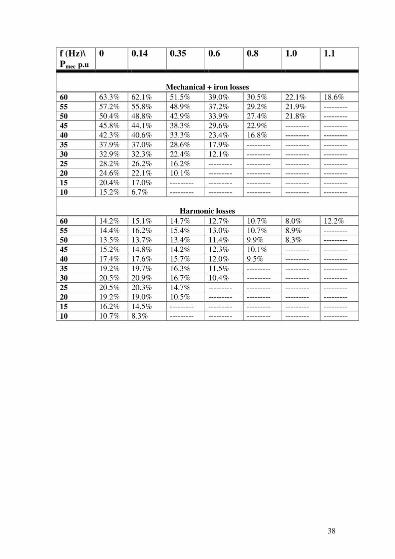
Mechanical + iron losses

60 63.3% 62.1% 51.5% 39.0% 30.5% 22.1% 18.6% 55 57.2% 55.8% 48.9% 37.2% 29.2% 21.9% --------- 50 50.4% 48.8% 42.9% 33.9% 27.4% 21.8% --------- 45 45.8% 44.1% 38.3% 29.6% 22.9% --------- --------- 40 42.3% 40.6% 33.3% 23.4% 16.8% --------- --------- 35 37.9% 37.0% 28.6% 17.9% --------- --------- --------- 30 32.9% 32.3% 22.4% 12.1% --------- --------- --------- 25 28.2% 26.2% 16.2% --------- --------- --------- --------- 20 24.6% 22.1% 10.1% --------- --------- --------- --------- 15 20.4% 17.0% --------- --------- --------- --------- --------- 10 15.2% 6.7% --------- --------- --------- --------- ---------

Harmonic losses

60 14.2% 15.1% 14.7% 12.7% 10.7% 8.0% 12.2% 55 14.4% 16.2% 15.4% 13.0% 10.7% 8.9% --------- 50 13.5% 13.7% 13.4% 11.4% 9.9% 8.3% --------- 45 15.2% 14.8% 14.2% 12.3% 10.1% --------- --------- 40 17.4% 17.6% 15.7% 12.0% 9.5% --------- --------- 35 19.2% 19.7% 16.3% 11.5% --------- --------- --------- 30 20.5% 20.9% 16.7% 10.4% --------- --------- --------- 25 20.5% 20.3% 14.7% --------- --------- --------- --------- 20 19.2% 19.0% 10.5% --------- --------- --------- --------- 15 16.2% 14.5% --------- --------- --------- --------- --------- 10 10.7% 8.3% --------- --------- --------- --------- ---------

39

6.1.2 The Warm Test This section presents the results from the measurements described in Section 5.5. The results from the cold test are also shown, so the results can be compared. All experiments described in this section were carried out with a constant output power of 3.2kW. Figure 6.1.2.1 shows the losses in the converter for the warm and cold.

Figure 6.1.2.1. The losses in the converter are almost the same for the cold and the warm test. The fact that the curves in figure 6.1.2.1 are approximately equal implies that the converter reaches its steady state temperature almost instantaneously. Figure 6.1.2.2 shows the efficiency of the IM. Obviously, the efficiency is lower when the motor is warm; the reason for this is that the losses in the rotor and stator are larger when the motor is warm, as is discussed below.

40

Figure 6.1.2.2. The efficiency of the motor is slightly lower for the warm tests. As in figure 6.1.1.8, a drop of the efficiency occurs at 50Hz. The difference between the two curves is approximately at 1.5-2%. The figure is a bit misleading at the points 42.5, 47.5 and 52.5 Hz since measurements at these points were only done in the warm test, not in the cold test. The stator and rotor losses are shown in figure 6.1.2.3 and 6.1.2.4 for the warm and for the cold IM.

41

Figure 6.1.2.3. The losses in the stator are higher in the warm test since the stator resistance has increased. As can be seen in figure 6.1.2.3, the stator losses are larger for the warm motor at steady state due to the temperature rise that has occurred. The resistance between two terminals was 2.8�-2.9� at steady state; the higher value occurred at the lower part of the frequency range. This can be compared with the terminal resistance when the motor is cold, which is 2.6 �. For example, at 40Hz the losses in the stator had increased 12% and the terminal resistance had increased 11.54%.

42

Figure 6.1.2.4. The losses in the rotor are higher in the warm test due to the increase of the rotor resistance. Figure 6.1.2.4 shows the losses in the rotor, which are higher for the IM at steady state for the same reason as the stator losses. The rotor losses increases after 52.5 Hz in a similar way as it did for the full load earlier. Figure 6.1.2.5 shows the harmonic losses in the IM. It can be noted that the losses in the warm test vary a lot. Why the variations arise has not been investigated.

Figure 6.1.2.5 The harmonic losses varies for an unknown reason. Figure 6.1.2.6 below shows the efficiency of the drive system.

43

Figure 6.1.2.6. The efficiency of the drive system is smaller in the warm test 6.2 Results from the IM Fed by a Converter of Type NFO Sinus This section presents the result from the tests, that where preformed in the same way as the measurements with the ABB converter in Section 6.1, with IM 1 and the converter of type NFO sinus. Measurements that gave similar results are left out in this section and can be found in Appendix 2. 6.2.1 The Cold Test The different losses in the IM have the same characteristic as for the ABB converter and are left out in this section. A comparison between the different setups is found in Section 9. The harmonic losses in the motor was found to be negligible, (their magnitude was approximately 1-2W), due to the fact that the NFO converter has a filter at its output, which reduces the harmonics. This results in higher losses in the converter; the losses are shown in figure 6.2.1.1 for different loads. It can be seen that the losses in the converter decrease as the frequency is increased; the reason for this was considered in Section 6.1.1. It can be noted that the losses are higher than before, which results in a lower efficiency, as can be seen in figure 6.2.1.2 below.

44

Figure 6.2.1.1 The losses in the converter decreases with increasing frequency

Figure 6.2.1.2 The efficiency of the converter is almost constant with regard to the output power when the output power is above 0.6 p.u. The efficiency reaches its maximum, 95%, at 60Hz and an output power of 0.8 p.u.

45

Figure 6.2.1.2 shows that the efficiency is almost constant after 0.6p.u and is increasing with increasing frequency. Figure 6.2.1.3 shows the efficiency of the IM at various output power. The efficiency is approximately 85-86% for loads over 0.35p.u and it has its maximum at an output power of 60Hz and 0.6p.u; this quite high value may be a bit misleading since the converter has a low efficiency due to its output filter.

Figure 6.2.1.3. The efficiency of the IM which has the maximum value at 60Hz and0.6 p.u output power where the efficiency is 87%.

46

Figure 6.2.1.4 The efficiency of the drive system is almost constant above an output power of 0.6p.u. Figure 6.2.1.4 shows the efficiency of the drive system and it can be noted that it does not increase much if the output power is increased beyond 0.6 p.u. The difference between the different loads above 0.6 p.u is approximately 3% of efficiency. It can also be concluded that the efficiency was a few percent better with the ABB converter; this will be discussed in in Section 9.1. 6.2.2 Warm test The same measurements that were performed with the ABB converter at steady state were also preformed with the NFO converter. The measurements with the NFO converter gave similar results as the measurements with the ABB converter described in Section 6.1.2. The results are found in appendix 2. The losses in the converter were found to be the same as for the cold test. The efficiency of the drive system is presented in figure 6.2.2.1. It can be seen that the efficiency is lower in the warm test; the reason for this is that the losses are higher.

47

Figure 6.2.2.1. The efficiency of the drive system is approximately 1-2% lower for the warm test

48

6.3 IM 1 fed by converter type Danfoss VLT 6000 This test was preformed in almost the same way as the test described in Section 6.1, and the results are presented in the following two sections. The difference was that no measurements were carried out at 10, 20, 30 and 40 Hz at full load, because a too high current was required for such measurements. The reason for this is that the Danfoss Converter does not operate at a constant voltage to frequency ratio (U/f) as the other two converters; therefore, the breaking point for the torque is not constant for different frequencies as it is when the voltage to frequency ratio is constant. The converter was connected after a transformer to overcome the problem with the circuit breaker releasing at high current leakage to ground. Results from the cold test and the warm test with the IM fed by a converter of type Danfoss will now be considered. 6.3.1 Cold test The results that gave results similar to those in Section 6.1.1 and 6.2.1 are left out in this section and can be found in appendix 2. Figure 6.3.1 shows the total input power to the IM at constant output power.

Figure 6.3.1.1. The output power deviation is 0.3%; it can be noted that the total input power decreases with increasing frequency. The mean deviation of the output was 0.3%, which for example, results in 9.6W at 3.2kW output power, which could be compared with 32W for the test with the ABB

49

converter. It can be noted that the input power decreases with increasing frequency due to the fact that the total loss component is decreased at higher frequency. Furthermore, the stator and rotor loss showed the same characteristic as before (see Section 6.1.1); the results from the stator and rotor loss measurements are therefore left out in this section. However, the iron losses differ a lot from the previous measurements, as can be seen in the figure 6. 3.1.2.

Figure 6.3.1.2. The mechanical and core losses at no load. The reason the core losses are relatively low in figure 6.3.1.2 compared to the core losses described in Section 6.1.1 is that the voltage is much lower with this converter, at no load. For example, at 50Hz and no load, the phase voltage was measured to 110.4V, and at full load to 225.5V. This change in the voltage leads to a large difference in the core losses since the core losses are proportional to the square of the voltage. The sum of the mechanical losses and the core losses at constant output power is shown in figure 6.3.1.3.

50

Figure 6.3.1.3. The core losses increases as the load increases and also with increasing frequency It can be seen that the core losses increases as the load increases, as expected since the voltage increases with increased load. The three curves are almost identical for the frequencies 55Hz and 60Hz at 0.8 p.u and 1.0 p.u. The reason for this is that the change in the voltage is almost negligible. Figure 6.3.1.4 and 6.2.1.5 show the efficiency of the IM and for the converter, respectively.

51

Figure 6.3.1.4. The efficiency of the IM where the efficiency is almost constant after 0.35p.u. As can be seen in figure 6.3.1.4, the efficiency does not increase much if the output power is increased above 0.35p.u, and the efficiency has its maximum at 60Hz and 0.8 p.u, where it is 87%.

Figure 6.3.1.5. The efficiency is almost constant after 0.35 p.u and has its higest efficiency of 97% at 60Hz and 1p.u output power. .

52

Figure 6.3.1.5 shows that the efficiency does not increase much if the output power is increased above 0.35 p.u, The maximum efficiency, 97%, is obtained at 60Hz and 1p.u output power. Table 6.3.1 shows the part of losses that were not accounted for in the measurements i.e the stray losses. However, as mentioned in Section 6.1, this is not an accurate value of the sray losses. Table 6.3.1 f\ Pmec p.u 0 0.14 0.35 0.6 0.8 1.0

)/()( mecinlossmecin PPPPP −−−

60 0.0% 1.2% 1.9% 5.0% 7.0% 9.9% 55 0.1% 0.8% 0.2% 3.2% 6.1% 8.4% 50 0.0% 1.7% 2.4% 5.7% 6.2% 5.4% 45 0.0% 0.8% 2.7% 4.2% 6.5% ---------- 40 0.0% 0.2% 2.4% 1.5% ---------- ---------- 35 0.0% 2.6% 1.5% 4.8% ---------- ---------- 30 0.0% 2.2% 1.6% ---------- ---------- ---------- 25 0.0% 1.4% 2.1% ---------- ---------- ---------- 20 0.0% 0.6% ---------- ---------- ---------- ---------- 15 0.0% 1.0% ---------- ---------- ---------- ---------- 6.3.2 The Warm Test This test was performed for the frequencies ranging from 44Hz to 56Hz in steps of 2Hz. The output power was at a constant level of 3.2kW, as in the warm test described in Section 6.1.2 above. The reason for the change in the frequency range compared to Section 6.1.2 was that the current became too large for lower frequencies. The result from this test was that the different types of losses showed the same characteristic as the losses found in the warm test described in Section 6.1.2. Graphs illustrating the results from the warm test described in this section are found in Appendix 2.

53

6.4 The No Load Test A no load test was preformed for the frequencies between 20 and 60Hz in steps of 5Hz, starting at 60Hz. The voltage was decreased to the point where the current increased. The blue curve in Figure 6.4.1 sows the no load power at 50Hz at varying phase voltage. The red curve shows the linear regression of the measured values

Figure 6.4.1 The measured value is almost identical as the liner regression. By using linear regression, the mechanical losses were calculated to 67.9 W. The mechanical losses in the IM1 were then calculated by subtracting the friction losses in the DC machine. The results are plotted in figure 6.4.2 below.

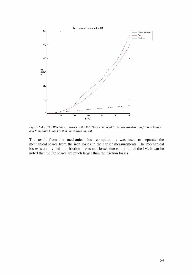
54

Figure 6.4.2. The mechanical losses in the IM. The mechanical losses are divided into friction losses and losses due to the fan that cools down the IM. The result from the mechanical loss computations was used to separate the mechanical losses from the iron losses in the earlier measurements. The mechanical losses were divided into friction losses and losses due to the fan of the IM. It can be noted that the fan losses are much larger than the friction losses.

55

7.0 Results IM 2 The measurements on IM2 were preformed in the same way as the measurements on IM 1. The results presented in this section also include the result from the measurements on IM 1 for comparison. Most of the measurement results are left out since they show the same characteristics as the characteristics presented in section 6; only results that show how IM1 and IM2 differs from each other are discussed. 7.1 The Cold test As mentioned above, this section focuses on the differences between IM 1 and IM 2 / between the two IMs. The stator losses and the rotor losses are presented in table 7.1.1 for an output power of 0.35 p.u. The difference between the two IMs is calculated as:

121 )( IMIMIM PPPdifference −= ,where PIMx refers to the loss component of IM number x.

Table7.1.1 Stator and Rotor losses in IM1 and IM2 Stator losses Rotor losses

f IM1 IM2 Difference IM1 IM2 Difference

25 246 263 6.9% 146 134 -8.2% 30 164 173 4.9% 86 77 -9.6% 35 125 128 2.4% 52 49 -5.2% 40 107 107 0.4% 46 39 -13.9% 45 93 95 1.7% 40 34 -13.5% 50 82 85 3.2% 35 30 -15.9% 55 74.8 78 3.7% 32 27 -15.6% 60 68 71 5.2% 28 26 -9.5% It can be noted that the total difference of the stator and rotor losses are negligible. It is also worth mentioning that the inaccuracy in the adjustment of the output power between the two machines was less than 0.1%, which means 1.4W at an output power of 0.35 p.u. Hence, the difference in the output power can be neglected. The mechanical losses and the core losses for IM 2 at 0.35 p.u are presented in table 7.1.2, together with the sum of the total losses in IM1 and IM2.

56

Table7.1.2 The mechanical, the core losses and the total losses in IM1 and IM2 Mechanical and core

losses Total losses, Pin-Pmec

f IM1 IM2 Difference IM1 IM2 Difference

25 46 51 14.1% 482 501 3.9% 30 56 61 11.1% 341 362 6.1% 35 60 76 10.1% 279 298 6.7% 40 73 87 19.0% 263 280 6.8% 45 79 94 19.3% 251 270 7.6% 50 88 103 16.7% 237 263 11.3% 55 92 109 18.7% 238 267 12.5% 60 105 123 17.4% 219 264 20.8% It can be noted that the difference in the losses between the two machines is due to the mechanical losses and the core losses (there were no significant difference for the harmonic losses). The difference in the mechanical and core losses is due to the fact that the friction in IM 2 is larger than the friction in IM 1. Figure 7.1.1 shows the efficiency of IM1 and IM2 for 0.35p.u and 0.8p.u.

Figure 7.1.1. The efficiency of IM1 andIm2 for 0.35 p.u and 0.8 p.u output power. Figure 7.1.1 shows that IM1 has higher efficiency than IM2. The reason for this is that the mechanical losses are larger for IM 2, as can be seen in table 7.1.2.

57

7.2 The Warm Test The warm test was preformed in the same way for IM2 as for IM1 and the results showed the same characteristic for IM 2 as for IM 1; therefore, the results are left out from this report.

58

8.0 Results of the converter measurements This section presents results from measurements that were performed on an ABB converter, an NFO converter and a Danfoss converter. Section 8.1 presents results from measurements on the ABB converter; the following two sections present results from measurements on the NFO converter and on the Danfoss converter. 8.1 The ABB Converter The measurements on the ABB converter were preformed as described in section 5.5 above. Figure 8.1.1 shows the phase voltage of the output from the converter for the IM running at 50Hz and 0.5p.u output power.

Figure 8.1.1. The phase voltage of the converter at 50Hz with the IM running at 50Hz and an output power of 0.5p.u. The rise time, the fall time and the switching frequency were measured, and they were found to be. trise=0.3µs tfall =0.1µs fsw =1kHz The calculation of the switching losses is left out due to the difficulties in establishing the DC voltage in the converter.

59

8.2 The Danfoss Converter The measurements on the Danfoss converter were preformed in the same way as with the ABB converter. Figure 8.2.1 shows the phase voltage at 50Hz and an output power of 0.5p.u.

Figure 8.2.1. The phase voltage of the Danfoss converter with the IM running at 50Hz and an output power of 0.5p.u. The rise time, the fall time and the switching frequency were: trise = 940 ns tfall = 925ns fsw = 4.5kHz As can be seen in figure 8.2.1, the switching characteristic changes at the voltage peaks. This is due to the fact that the converter stops switching at the peaks. This results in lower switching losses, which is desirable, but also in a larger harmonic content. However, since the phase voltage characteristics only changes for a relatively short period at the peaks, the increase of the harmonics is not large. The calculation of the switching losses will be left out because of the same reason mentioned in section 8.2.

60

8.3 The NFO Converter The measurement procedure described in Section 8.2 above was not applicable to the NFO converter, since the converter has a filter at its output. The phase voltage of the NFO converter used in the measurements is shown in figure 8.3.1. The IM was running at 50Hz and 0.5 p.u output power. It can be noted that the waveform is almost sinusoidal.

Figure 8.3.1. The phase voltage when the IM is running at 50Hz and 0.5p.u output power.

61

9.0 Comparison of the Converters This section will present a comparison of the three types of converters discussed above. Comparisons were made both when the converters were feeding IM 1 and when they were feeding IM 2. The results from the comparisons using IM 1 are presented in Section 9.1 below, and the results from IM 2 are presented in Section 9.2. 9.1 Converters feeding IM 1 A comparison between the three converters was preformed in order to establish the different loss components. Figure 9.1.1 shows the stator losses in the IM for two different loads. The curves with the higher value belong to 0.6p.u output. The figure indicates that the difference between the three converters decreases as the output power increases. The figure also shows that the ABB converter generally produces the highest losses and the Danfoss converter the lowest losses.

Figure 9.1.1. The three curves in the upper right part of the figure shows the stator losses for an output power of 0.6p.u; the three curves in the lower left par of the figure shows thelosses for 0.14 p.u. The stator losses are generally higher in the ABB converter and lower in the Danfoss converter. Figure 9.1.2 shows the losses in the rotor for the same situation as above. The figure shows that the ABB converter, which has the highest stator losses, produces the lowest rotor losses while the Danfoss converter, which produces the lowest stator losses, produces the highest. However, the sum of the resistive losses is higher for the ABB converter.

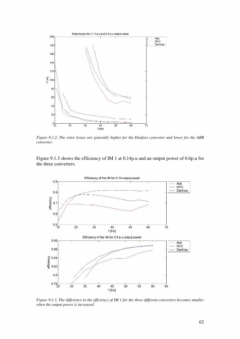
62

Figure 9.1.2. The rotor losses are generally higher for the Danfoss converter and lower for the ABB converter. Figure 9.1.3 shows the efficiency of IM 1 at 0.14p.u and an output power of 0.6p.u for the three converters.

Figure 9.1.3. The difference in the efficiency of IM 1 for the three different converters becomes smaller when the output power is increased.

63

It can be seen that the difference in the efficiency decreases as the load increases and that the ABB converter has the lowest efficiency while Danfoss has the highest. The efficiency of the IM for the NFO converter is a bit miss-leading since, as noted in section 6, the NFO converter has a relatively low efficiency. Figure 9.1.4 and 9.1.5 show the efficiency of the converters and the drive system, respectively.

Figure 9.1.4. The ABB converter has the highest efficiency while the NFO converter has the lowest…. As can be seen in figure 9.1.4, the NFO converter has the lowest efficiency, which was expected since it has a filter on its output. It can also be noted that the ABB converter has the heighest efficiency, but it also has the highest harmonic content, according to the result presented in section 6.1.1.

64

Figure 9.1.5. The efficiency of the drive system for 0.14 p.u and 0.6 p.u output power. The difference decreases as the load increases and the Danfoss converter produces the highest efficiency. Figure 9.1.5 shows that the Danfoss converter has the highest efficiency and that the differences between the converters are larger at light loads. This was an expected result since the Danfoss converter optimizes the power consumption, which has a greater influence at light loads. 9.2 Converters feeding IM 2 The results from the measurements on IM 2 are similar to the results from the measurements on IM 1, and they are therefore left out from this repport.

65

10.0 Field measurements This section will present the accuracy of measurements done with the slip method, the current method and the air gap torque method. The tests were preformed at 50Hz and with IM 2 connected to the line supply. The output torque was measured for comparison with different methods. The load was varied from 1kW to 4kW in steps of 0.5kW. 10.1 The slip method The rated speed was 1435 rpm and the rated output power of 4kW. From this data the output torque could be estimated. However, the results obtained from the slip method (equation 3-14) were quite inaccurate; the difference in the efficiency was 10-20%. For example, the most accurate result from the slip method was that the efficiency at full load should be 77%, but in fact it was 84% (according to the measured value). However, this method was not expected to be very accurate, as mentioned in section 3.4.1. The measured speed at full load was 1441, which results in a difference of 9% from the rated slip. Using this value in the calculations resulted in no significant improvement. 10.2 The current method According to the IM nameplate, the rated current was 8.9A and the rated output power 4kW. With the rated current and the rated output power known, the current method (equation 3-19) could be used to estimate the efficiency. The difference between the actual efficiency and the efficiency according to the current method was 4% at full load, which was the most accurate estimate obtained from the current method. One reason for the inaccuracy in the measurements is that the measured rated current was 8.72A, not 8.9A (as the nameplate of the IM indicated) that is a difference of 2%. However, the current method was not expected to be very accurate, as explained in section 3.4.2. 10.3 The air gap torque method The phase voltages, the line currents and the stator resistance were measured after each load situation. The data was processed in Matlab, as described in section 3.4.3, to establish the air gap torque. Figure 10.3.1 shows the air gap torque and the measured torque.

66

Figure 10.3.1. The output power varies from 0.25 p.u to 1 p.u in steps of 0.125p.u. Figure 10.3.1 shows an almost constant difference between the measured torque and the calculated air gap torque. The reason for the difference is that the mechanical, the core and the rotor losses are not accounted for in the air gap torque method. In order to take those losses into account, the no load power was measured, and the mechanical losses and the core losses were calculated according to Section 5.3 and subtracted from the air gap torque. Furthermore, the rotor losses were calculated using equation 3-9. The result showed a difference between the measured and calculated torque of approximately 0.5% The estimated efficiency and the measured efficiency are presented in figure 10.3.2.

67

Figure 10.3.2. The blue line shows the air gap torque efficiency with the mechanical losses, the core losses and the rotor losses subtracted from the air gap power. The red line shows the measured efficiency. The table next to the plot shows the relative difference between the calculated and the measured efficiency (�meas /�airgap) Figure 10.3.2 shows that the difference between the calculated efficiency according to the air gap torque method (with the mechanical, core and rotor losses taken into account) and the measured efficiency is relatively small. The table on the right in figure 10.3.2 shows the relative difference between the estimated value and the measured value (�meas /�air gap). It may not be possible to run the no load test in the industry. If this is the case the mechanical, core and rotor losses have to be estimated, which results in a more inaccurate result [7].

68

10.4 Comparison of the Three Methods The measurements show that the air gap torque method is the most accurate method for estimating the efficiency. Unfortunately, it is also the method with the largest intrusion level, since the IM has to be running at no load if the mechanical, core and rotor losses are to be measured. However, these quantities can be estimated. The slip method and the current method are more accurate at high loads; at low loads, they are quite inaccurate compared to the air gap torque method. However, these methods are not recommended to use even at high loads due to their inaccuracy.

69

11.0 Conclusions This report has considered the different losses in a drive system consisting of an IM fed by a frequency converter and how the different loss component varies with the frequency at different loads. The measurements where performed on two different IMs fed by three different types of converters. It was concluded that the different loss components in the system could be determined fairly accurrately. However, the stray loss measurement resulted in a relatively high inaccuracy and it was concluded that the value differed approximately 50% from other documentation on the stray losses. Furthermore, the loss components showed the same characteristic between the different types of converters. However, the core losses in the Danfoss converter were lower due to the decrease in the voltage at light loads. It has also been shown that the Danfoss converter generally provides the best efficiency of the drivesystem where the diffrence became higher at light loads. However, the highest efficiency was found when the IM was fed with the ABB converter. The highest efficiency of the drive system occures at 60Hz and 0.8 p.u where values of 83.8%, 81.5% and 83.7% was establiched for the ABB, the NFO and the Danfoss converter, respectively. The result from the measurements on IM2 showed the same caracteristic as the results from the measurements made on IM1 and the different losses was almost identical. However, IM2 showed a slightly lower efficiency due to the higher value of the mechanical loss as mentionend in section 7.1. It can also be concluded that the field method with the highest accuracy is the air gap torque method. This method resulted in a 0.5% difference from the measured torque. The test is intrusive if measurements of the mechanical and core losses are done on an IM at no load, but, as mentioned in section 10.3, these queantities can be estimated at the cost of decreased accuracy [7].

70

List of symbols DC machine Ua armature voltage [V] Ia armature current [A] If field current [A] Pµdc mechanical losses in the DC machine [W] TL load torque [Nm] Induction machine ULL line-to-line voltage [V] Uph phase voltage [V] Ia,Ib Ic line currents in phase a, b and c [A] I line mean value of the line current [A] I rated rated line current [A] I(1) fundamental line current [A] I0 mean value of the no load line currents [A] Rs stator resistance [�] Rdc dc resistance between two terminals [�] Rr rotor resistance [�] Rc representation of mechanical and core losses [�] Lm magnetizing inductance [H] Ls stator leakage inductance [H] Lr rotor leakage inductance [H] f supply frequency [Hz] Pin total input electrical power [W] Pin(1) fundamental component input power [W] Pmec mechanical output power [W] Prated rated mechanical output power [W] P� airgap power [W] P0 no load power [W] Pstator resistive losses in the stator [W] Protor resistive losses in the rotor [W] Pcm mechanical +core losses [W] Pcore core losses [W] PµIM mechanical losses [W] Pharmonic harmonic losses [W] Pstray stray loss [W] Tmec output torque [Nm] T� air gap torque [Nm] n rotor speed [rpm] ns synchronous speed [rpm] � rotor speed [rad/s] �s synchronous speed [rad/s] s slip [] p numer of poles

71

Induction and DC machine Pµ the total mechanical losses [W]

Converter Pf electric input power [W] Pe1 electric output power measured with [W]

Yokogawa power analyser Pe2 electric output power measured with [W]

Norma power analyser Udc the DC voltage in the converter [V] trise rise time [s] tfall fall time [s] fsw switching frequency [Hz] Psw switching losses [W]

72

Appendix 1 Equation 11 in section 3.3 can be derived as follows: �∆−−∆+=∆+ outoutininlossloss PPPPPP (A1-1)

�∆−∆=∆�−−+∆−∆=∆

outsinloss

lossoutinoutsinloss

PPP

PPPPPP (A1-2)

�∆+∆≤∆−∆=∆ outinoutinloss PPPPP (A1-3)

�

�

��

�

=

=�

−∆+∆

=∆+∆

≤∆

η

ηout

in

inout

outin

outin

loss

outin

loss

loss PP

PP

PP

PP

P

PP

P

P (A1-4)

�−

∆+

−∆

≤∆

)11

()1(η

ηout

out

in

in

loss

loss

P

PP

PPP

(A1-5)

)1(,1

11

1 <���

����

� ∆+

∆−

<���

����

� ∆+

∆−

≤∆

ηηη in

in

out

out

in

in

out

out

loss

loss

PP

PP

PP

PP

P

P (A1-6)

73

Appendix 2 The results left out in section 6 are presented in the following sections. NFO cold test Figure A2-1 shows the total input power to the IM at constant output power.

Figure A2- 1. The electrical input power at constant output power Figure A2-2 and A2-3 shows the stator and rotor losses.

74

Figure A2-2. The losses in the stator decrease with increasing frequency.

Figure A2-3. The rotor losses decrease with increasing frequency except at 1 p.u.output power.

75

As mentioned above, figure A2-3 shows the rotor losses at constant output power. It can be noted that the losses increase with the frequency when Pmec =1p.u. The same result was obtained in the measurements with the ABB converter. Figure A2-4 shows the mechanical losses and the core losses at no load.

Figure A2-4. The core losses decreases after 50Hz since the voltage settles. The reason the losses cease to increase at 50Hz is the same reason as the one mentioned in section 6.1.1, namely that the voltage does not increase further and, hence, the iron losses decrease, since the voltage to frequency ratio decreases. The input and the output power at 60Hz are shown in the upper part of figure A2-5. The sum of the output power and the calculated losses is also plotted for comparison. In the lower part of the figure the losses in the IM are plotted.

76

Figure A2-5. The part of the losses that are not accounted for is approximately 5-10%. The part of the losses that is not accounted for in this figure is approximately 5-10% where 10% is the value for the highest load. NFO warm test The same measurements that was preformed for the ABB converter at steady state was also preformed with the NFO converter. The results are presented below. The stator and the rotor losses are presented in figure A2-6 and A2-7 respectively.

77

Figure A2-6. The losses in the stator are higher in the warm test since the stator resistance has increased.

Figure A2-7. The losses in the rotor are larger in the warm test due to the temperature rise in the IM.

78

Figure A2-7 shows the losses in the rotor. It can be noted that the rotor losses increases after 52.5Hz as for the test with the ABB converter discussed in section 6.1.2. Danfoss Cold test Figure A2-8 and A2-9 shows the losses in the stator and rotor, respectively.

Figure A2- 8. The stator losses decrease with increasing frequency.

79

Figure A2-9. The losses in the rotor decrease with increasing frequency, except for an output power of 1 p.u. Figure A2-9 shows the rotor losses at constant output power. It can be noted that the losses increase for 1p.u output power for the frequencies 55 Hz and 60Hz, as was noted in in Section 6.1.1. The upper part of figure A2-10 below shows the input and output power at 60Hz, and the sum of the output power and the losses. The difference between the input power and the sum of the output power and the calculated losses at full load is 12.5%; this difference decreases with decreasing frequency and load.

80

Figure A2-10. The upper part shows the mechanical output power, the input power and the sum of the input power and the calculated losses. The lower part shows the different loss components in the IM. Danfoss warm test This test was preformed for the frequencies ranging from 44Hz to 56Hz in steps of 2Hz. The output power was 3.2kW throughout the test. Figure A2-11 presents the losses in the converter for the cold and the warm test. It can be seen that the difference between the losses for the warm and cold test are neglectable.

81

Figure A2-11. The losses in the converter are approximately the same for the cold and the warm test. Figure A2-12 and A2-13 below show the losses in the stator and the rotor, respectively. It can be seen that the resistive losses are larger in the warm test. This is due to the fact that resistance in the stator and the rotor increases with increasing temperature.

82

Figure A2-12 The losses in the stator has decreased in the warm test due to the increase of the stator resistance.

Figure A2-14 shows the efficiency of the IM. It can be noted that the efficiency is lower in the warm test. The reason for this is the increase in the resistive losses that were presented in figure A2-12 and A2-13.

83

Figure A2-14. It can be noted that the efficiency of the IM is lower for in the warm test.

84

References [1] Cao-Minh and Yoichi Hori , ”Convergence Improvement of efficiency-Optimization control of induction motor drives” IEEE Transactions on Industry Applications vol.37 NO 6 Nov/Dec 2001 [2] “IEEE Standard test Procedure for Polyphase Induction Motors and generators”, March 10 1991 [3] Ned Mohan “Electric Drives an integrative approach” 2003 pp 15-1 to 15-12 [4] “Elteknik” department of Electric Power Engineering p 102 [5] http://www.national.com/appinfo/power/files/LM5030_Push-Pull-12V-60W.pdf, 2004-09-01 [6] Joachim Lindström,”Development of an experimental permanent magnet motor drive” 1999, p162. [7] John S. Hsu, John D Kueck, Mitchell Olszewski, Don A Casada, Pedro J. Otaduy and Leon M. Tolbert “Comparation of Induction Motor Field Efficiency Evaluation Methods” IEEE Transactions on Industry Applications vol.34 NO 1 Jan/Feb 1998 [8] J. S.Hsu , H. H. Woodson and W. F. Weldon, “Possible errors in measurement of air-gap torque pulsations of induction motors” IEEE trans. Energy Conversion, vol. 7 no 1 pp 202-208 Mars 1992 [9] Ned Mohan, Tore M. Underland and William P. Robbins “Power electronics” third edition, 2003, pp-399-431, ISBN 0-471-22693-9 [10] Austin Hughes, “Electric motors and drives fundamentals, types and applications” second edition, 1993, p-297, ISBN 0-7506-1741-1 [11] Paolo Bertoldi, Anibal de Almedia and Hugh Falkner, “Energy efficiency improvements in electric motors and drives”, 2000, p82, ISBN 3-540-67489-6 [12] Esam Hamdi, “Permanent magnet and variable reluctance systems” 2003 pp 64-76, ISBN 91-974614-0-7 [13] http://www.nema.org/engineering/icsstandards/acadjustable.pdf 2004-09-10 [14] http://138.227.174.121/GLOBAL/SCOT/scot259.nsf/0/98c7337232271ef6c1256 bab00668ba4/$FILE/ATT4XBB6/The%20Motor%20Guide%20GB.pdf ,2004-09-22 [15] B. Reiner, K. Hameyer, and R. Belmans, “Comparison of standards for determining efficiency of three phase induction motors”, IEEE Transactions on Energy Conversion Vol. 14 No. 3, September 1999.