Measurement of DRAM Prices: Technology and Market · PDF file5 Measurement of DRAM Prices:...
51
This PDF is a selection from an out-of-print volume from the National Bureau of Economic Research Volume Title: Price Measurements and Their Uses Volume Author/Editor: Murry Foss, Marylin Manser, and Allan Young, editors Volume Publisher: University of Chicago Press Volume ISBN: 0-226-25730-4 Volume URL: http://www.nber.org/books/foss93-1 Conference Date: March 22-23, 1990 Publication Date: January 1993 Chapter Title: Measurement of DRAM Prices: Technology and Market Structure Chapter Author: Kenneth Flamm Chapter URL: http://www.nber.org/chapters/c7802 Chapter pages in book: (p. 157 - 206)
Transcript of Measurement of DRAM Prices: Technology and Market · PDF file5 Measurement of DRAM Prices:...
This PDF is a selection from an out-of-print volume from the National Bureauof Economic Research
Volume Title: Price Measurements and Their Uses
Volume Author/Editor: Murry Foss, Marylin Manser, and Allan Young, editors
Volume Publisher: University of Chicago Press
Volume ISBN: 0-226-25730-4
Volume URL: http://www.nber.org/books/foss93-1
Conference Date: March 22-23, 1990
Publication Date: January 1993
Chapter Title: Measurement of DRAM Prices: Technology and Market Structure
Chapter Author: Kenneth Flamm
Chapter URL: http://www.nber.org/chapters/c7802
Chapter pages in book: (p. 157 - 206)

5 Measurement of DRAM Prices: Technology and Market Structure Kenneth Flamm
Semiconductor memory is an example of a good undergoing continuing, rapid technological change, with historical price declines even more dramatic than in the (now well-documented) case of computers. Indeed, declines in the cost of memory are most likely a major cause underlying the striking behavior of computer prices.
A twenty-year downward spiral in memory prices came to an abrupt halt in 1987. For the first time in the recorded history of the chip industry, substantial and sustained increases in memory costs were noted in 1987 and 1988. Al- though the reason for these increases is not the focus of this paper, it is reason- able to suspect that the negotiation of the Semiconductor Trade Arrangement (STA) between the United States and Japan, which became operational in late 1986, may have catalyzed this abrupt reversal of historical trends (see Flamm 1989, 1990, 1993).
This paper was motivated by my difficulties in determining exactly what happened to memory prices in 1987 and 1988 and what the probable effect of these price increases was on computer systems prices. It is concerned primar- ily with the task of analyzing price indexes for the computer memory chip type that accounts for the vast bulk of the market, the so-called dynamic ran- dom access memory (DRAM). Existing data on DRAM prices suffer from many deficiencies, most of which are detailed below (although not all are remedied). Producer price indexes prepared by the Bureau of Labor Statistics
Kenneth Flamm is a senior fellow at the Brookings Institution, Washington, D.C. Without implicating them in his errors, the author thanks Marilyn Manser, Jack Triplett, Ellen
Dulberger, Philip Webre, Doug Andrey, and Mark Giudice for their useful comments and sugges- tions and Yuko Iida Frost for very helpful research assistance. The views expressed in this paper are the author’s alone and in no way represent those of the officers, trustees, or staff of the Brook- ings Institution.
1. For a comprehensive survey and synthesis of studies of computer prices, see Triplett (1989a).
157

158 Kenneth Flamm
(BLS) suffer from critical problems described below and in Dulberger (chap. 3 in this volume). By default, estimates prepared by the market consulting firm Dataquest are the most commonly used source of price data in this indus- try (they are used by Dulberger and even published in the official Statistical Abstract of the United States).
For this reason, I examine the methodology underlying the Dataquest price estimates in some detail in this paper. Rather than rely on the Dataquest fig- ures, this paper develops new time-series data on DRAM prices from data on individual transactions and presents an econometric analysis of pricing prac- tices within the market that enables us to control for relevant characteristics of the product and the transaction. Approximate Fisher Ideal DRAM price in- dexes using this new data are also constructed; these research price indexes may be of use in future work on this important industry.
I begin with a discussion of the nature of the product, its technology, and the industrial organization of the DRAM market. Then follows an examina- tion of existing data on DRAM pricing and the strengths and weaknesses of different statistical sources. This is followed by an econometric analysis of a sample of actual DRAM contracts, from which both a price index and some suggestive analysis are then extracted.
5.1 The Product and Its Technology
Memory chips are the largest single segment in the U.S. semiconductor market, accounting for 28 percent of sales in 1989; they accounted for 34 percent of integrated circuit (IC) consumption.2 The dominant product (with almost two-thirds of memory sales) was the DRAM, which by itself ac- counted for 20 percent of American IC consumption in 1989.
The first widely used commercial DRAM was the 1K memory (K means 1,024 bits of information), introduced in 1970 by American semiconductor companies. A new generation chip (with four times the capacity of the last generation) has been introduced approximately every three years since the mid- 1970s.
At center stage in the continuing saga of technological improvement in DRAMs sits continuing advance in semiconductor manufacturing processes. Improvements in fabrication technology have steadily reduced the size of electronic circuit elements and stimulated development of fabrication pro- cesses for novel types of physical microstructures implementing standard electronic functions.
The principal and overwhelmingly important characteristic of a DRAM from the point of view of its consumers is its bit capacity, the amount of infor-
2. These figures are based on U.S. market estimates from Electronics, January 1990, 83. Note that only a small fraction of DRAMs consumed are manufactured within the United States; DRAMs account for a much smaller share of the value of U.S. production.

159 Measurement of DRAM Prices: Technology and Market Structure
mation it can hold. The effect of technical improvement is typically measured in cost per bit. Greater density would be more desirable even in the absence of reduction in bit cost, however, because fewer chips must be interconnected within a system, lowering system manufacturing costs.
Faster access speed is also of importance to users but, like manufacturing cost per bit, is highly correlated with circuit density over the long run. Higher density parts are generally considerably faster than older parts; the shorter lengths of connections between circuit elements improve speed.
DRAMs are generally designed with some “standard,” average speed spec- ification in mind. Typically, the result of the fabrication process is a bell- shaped distribution around the specified speed, at which the chips perform adequately. The chips residing in the left tail of the distribution are identified through testing; those not meeting the design specifications have their speed ratings reduced and are sold at a discount.
As fabrication technology continuously improves, chip size is shrunk. Three or more such “die shrinks” may typically occur over the life cycle of a given capacity DRAM within a single company. A desirable side effect of incrementally smaller chips is gradually improved speed. Thus, the speed of the “standard” 256K DRAM produced by most manufacturers went from 150 to 120 nanosecond (ns) access time over the period 1987-88, the result of die shrinks. Even improvements in manufacturing processes for an existing de- sign have often been associated with changes in product specifications large enough to lead to reclassification as new product types.
Chips also use power, and lower power consumption is desirable. It means less costly power supplies, and costs for heat dissipation, within systems that use chips. Beginning with the 64K generation, a lower-power chip technology known as CMOS (complementary metal-oxide semiconductor) gradually be- gan to displace an older technology (known as NMOS [n-channel metal-oxide semiconductor]) in DRAM manufacture. The introduction of the 1M (for megabit, 1,024K) DRAM marked the almost complete displacement of NMOS by CMOS technology in DRAM manufacture, so power consumption is rarely an important factor in selection among current generation chips.
Because improvements in virtually all the desirable characteristics of DRAMs have been positively correlated with lower bit cost, cost per bit can probably be regarded as an upper bound on a suitably defined index of quality- adjusted chip cost. Data presented later in this paper show that, over at least some time periods, changes in simple cost per bit, for chips of given memory capacity, have not diverged greatly from a superlative DRAM price index ac- counting for technical improvements in speed and organization as well.
A crucial point to make is that virtually all technological improvement in DRAMs has been embodied in the introduction of distinct and identifiable new products, as opposed to more subtle qualitative improvement in existing chips. Because of this, construction of a price index that properly identifies and accounts for the introduction of new, improved products will also cor-

160 Kenneth Flamm
rectly capture the effect of technological advance (and other factors) on the cost of that input.
5.1.1 Product Differentiation DRAMS-and other memory chips-have a reputation as the “commod-
ity” product par excellence within the semiconductor industry: a high- volume, standardized good, with almost perfect substitution among different manufacturers’ offerings the norm. Chips from different manufacturers use the same array of package types, pins, and have many common minimal technical specifications. They mainly use the same speed classifications (rated in nano- seconds average access time to a bit). Products with appropriate specifications from different manufacturers may be substituted within a given piece of equip- ment. Although DRAMs are in this sense a “commodity” product, the actual physical design of the chip’s internal structures and many subtle aspects of its performance vary by manufacturer.
Because of subtle but important variation across producers in DRAM elec- trical and physical performance parameters, large manufacturers typically put a device through an extensive and expensive qualification p r o ~ e s s . ~ Some re- testing is required every time the manufacturing process for a chip is changed. These costs provide an important economic incentive for systems manufactur- ers to limit the number of qualified suppliers for a particular application. Quality standards maintained by a manufacturer reduce the need to test com- ponents after purchase, and DRAMs are generally shipped to large customers in boxes with quality seals to guarantee factory-set standards (physical han- dling of chips is a major cause of failure or degradation). Purchasing chips from a new supplier, or outside manufacturer-controlled sales channel^,^ will generally lead to expensive additional testing.
Until recent years, DRAM manufacturers did not differentiate their prod- ucts much in any dimensions other than speed and quality/reliability. This began to change in a significant way with the 64K generation of DRAMs, first shipped in 1979 (see Flaherty and Huang 1988, 12). The organization of chips (the way in which memory is accessed) began to diversify: a 1M DRAM, for example, may now be purchased in 1M X 1 or 256K X 4 con- figurations. New, specialized addressing structures were increasingly ~ f f e r e d . ~ And specialized, proprietary DRAM designs with application-specific fea- tures became increasingly common: line buffers for television and video use,
3. Merely qualifying and testing a second source for a part already in use was estimated by one industry source to cost $120,000. Qualification costs were large enough to prompt at least one group of relatively large computer manufacturers to form a cooperative chip qualification joint venture, in order to pool these costs. Within the electronics purchasing community, talk of the economic pressure to reduce the number of suppliers is a staple of everyday conversation.
4. Unless, as sometimes happens, the chips can be purchased in boxes with the original factory quality seals intact.
5 . Manufacturers of DRAMs now typically offer products with “page,” “fast page,” “nibble,” and “static column” addressing modes.
161 Measurement of DRAM Prices: Technology and Market Structure
multiple-ported buffers for computer graphics applications, bidirectional data buffers. Finally, a bewildering alphabet soup of package types is now used to encase a finished DRAM. There are many types of single-chip plastic casing for DRAMs,~ ceramic cases, and various kinds of multichip memory module packages.
Organization, addressing structures, and application-specific designs mark off substantially different products. Although they may be created on the same production line, different tooling, fabrication steps, and manufacturing prob- lems characterize these products. Packaging, on the other hand, can probably be regarded as a nonessential difference among chips. At a relatively late stage in the fabrication process, decisions can be made to change the mix of pack- ages used for the product. Indeed, competition among manufacturers works to drive costs for a DRAM toward the market price for that DRAM in the standard plastic case, plus some incremental add-on reflecting the cost to the producer of additional packaging options. If demand for a single specific package type exceeds supply, pushing price up, manufacturers can easily switch output to that package type quite late in the production process.
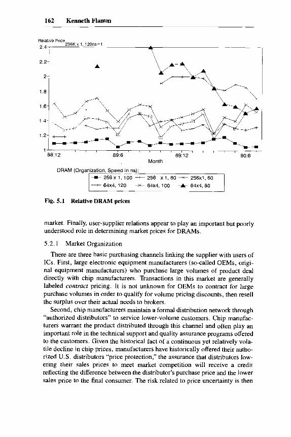
Note that the relative prices of DRAMs of varying sizes and organizations are quite volatile and do not seem to be linked by a particularly stable relation, even within the course of a single year. In particular, faster parts are typically introduced at a substantial premium relative to lower-speed components; this premium rapidly erodes over time, however, as the mix of output shifts toward faster chips, for reasons discussed next. Figure 5.1 shows the retail prices of various DRAMs relative to a garden variety 265K x 1, 120 ns part, as re- ported in advertisements by one Los Angeles-area mail-order vendor over the course of a year.’ Relative prices fluctuated quite a lot (note the rapid erosion in fast 60 ns 256K X 1 and 80 ns 64K X 4 chip prices relative to more ma- ture products).
5.2 Industrial Organization of the DRAM Market
Different classes of consumers purchase DRAMs through different sets of marketing channels. The distinctions are important: over the last half decade, price movements in each of these distinct market segments have varied greatly. Government policies seem to have accentuated these differences and created sharp regional (i.e., the United States, Europe, Japan, Asia, etc.) price differentials in what seems to have been a previously well-integrated
6. The most common was the familiar dual in-line pin (DIP), but there is also the single in-line pin package (SIPP), the zig-zag-in-line pin (ZIP), the small outline J-leaded (SOJ) case, and the plastic-leaded chip carrier (PLCC).
7. The vendor is L.A. Trade, and the source for these prices is the publication Computer Shop- per. Scrutiny of dated advertisements elsewhere in this publication suggests a two-month lag between submission of advertising copy and the month of publication for the magazine. The prices shown here are assigned to their inferred submission dates.
162 Kenneth Flamm
Relative Price
2,4 256Kx 1, 120ns=1
7
2.2- A
2-
1 8 -
Month
DRAM (Organization, Speed in ns): +256x1,100 +256 xl ,80+256x1,60 I
1 -if 64x4, 120 x 64x4, 100 t 64x4, 80 I
Fig. 5.1 Relative DRAM prices
market. Finally, user-supplier relations appear to play an important but poorly understood role in determining market prices for DRAMS.
5.2.1 Market Organization There are three basic purchasing channels linking the supplier with users of
ICs. First, large electronic equipment manufacturers (so-called OEMs, origi- nal equipment manufacturers) who purchase large volumes of product deal directly with chip manufacturers. Transactions in this market are generally labeled contruct pricing. It is not unknown for OEMs to contract for large purchase volumes in order to qualify for volume pricing discounts, then resell the surplus over their actual needs to brokers.
Second, chip manufacturers maintain a formal distribution network through “authorized distributors” to service lower-volume customers. Chip manufac- turers warrant the product distributed through this channel and often play an important role in the technical support and quality assurance programs offered to the customers. Given the historical fact of a continuous yet relatively vola- tile decline in chip prices, manufacturers have historically offered their autho- rized U.S. distributors “price protection,” the assurance that distributors low- ering their sales prices to meet market competition will receive a credit reflecting the difference between the distributor’s purchase price and the lower sales price to the final consumer. The risk related to price uncertainty is then

163 Measurement of DRAM Prices: Technology and Market Structure
assumed by the chip manufacturer. Pricing generally seems to be on a spot basis, although there can be a substantial lead time between orders and deliv- eries in times of buoyant demand, and distributor prices take on a “contract” aspect.
Finally, there is the so-called grey, or spot, market. Independent distribu- tors, brokers, and speculators buy and sell lots of chips for immediate deliv- ery. There is also a significant retail market selling directly to computer resell- ers and users wishing to upgrade computer systems or replace defective parts. Supplies of chips on the American grey market come from chip manufactur- ers, OEMs, and authorized distributors selling their excess inventories and also from Japanese trading companies and wholesalers purchasing directly from Japanese DRAM manufacturers (see, e.g., USITC 1986, A-12). Grey market product is not warranted by the manufacturer and has frequently been subjected to unknown handling and quality assurance procedures.
In 1985, U.S. industry sources estimated that authorized distributors ac- counted for about 30 percent of chip manufacturers’ DRAM sales (USITC 1985, A10-A1 1). Since grey market sales are often resales of product origi- nally sold through OEM contracts or authorized distributors and double count chips flowing into the grey channel from sources other than chip manufactur- ers, one must be careful in calculating the share of these different channels in sales to final users. One 1985 estimate held that 20 percent of “the mar- ket” (presumably, end users) is accounted for by the grey channel in times of shortage.
This is roughly in sync with more recent estimates. In early 1989, one in- dustry source estimated that perhaps 70 percent of DRAM sales were “con- tract” sales made directly by producers to large users, 15 percent went to final users through authorized distributors, and an additional 15 percent went through the grey market.8
5.2.2 Government Policy and Regional Segmentation of the Market A final factor complicating discussion of DRAM prices was the appearance
of significant regional price differentials in 1987 and 1988, after the signing of the STA. In response to the STA, the U.S. and Japanese governments began to set floor prices for export sales of DRAMS by Japanese companies. Initially, different standards were set for sales to the U.S. market and other (“third- country”) export markets; after U. s. protests, the systems were later unified. (In response to European protests, the pricing guidelines were separated again in 1989.)
Regulation of Japanese export sales ultimately involved four elements. First, an export licensing system was adopted. This system required de facto government approval of the export price, which was to be set above minimum
8 . The estimate is that of Don Bell, of Bell Microproducts Inc., whom I thank for spending the morning of 16 February 1989 attempting to educate me in the intricacies of the DRAM market.

164 Kenneth Flamm
norms established by Japan’s Ministry of International Trade and Industry (MITI). Second, foreign purchasers of Japanese chips were required to regis- ter with MITI. Third, all export transactions required a certificate provided by the original chip manufacturer attesting to the fact that the chips in question were actually manufactured by that producer. Fourth, MITI established infor- mal regional allocation guidelines to ensure that supplies were not diverted from one export market to favor another.
By most accounts, MITI’s guidance was quite effective in setting minimum pricing standards for Japanese DRAM manufacturers’ direct export sales. (Because Japanese manufacturers were by this time responsible for between 80 and 90 percent of world DRAM sales, this effectively worked as a floor on price in the global market.) The intent of the second and third elements was clearly to reduce access by foreign purchasers to Japanese grey market chan- nels not under the direct supervision and control of Japanese chip manufactur- ers. Predictably, prices in the unregulated Japanese market soon dropped be- low foreign export prices. In 1988, articles in the Japanese business press (see the references to them in Flamm [ 19931) suggested that the differential be- tween domestic and export pricing was quite large.
5.3 Historical Data on DRAM Prices: A Review and Comparison
At a relatively aggregate level of detail, BLS publishes matched-model pro- ducer price indexes for integrated circuits, including an estimated index for MOS memory. It is obvious to all those familiar with pricing behavior in the industry, however, that the BLS price indexes grossly underestimate price de- clines in entire classes of semiconductor products subject to rapid technologi- cal change, such as memory chips. (For example, the BLS producer price index for MOS memory ICs declines by about 50 percent over the five-year period from June 1981 to June 1986, implying an annual rate of price decline of only 13 percent .)
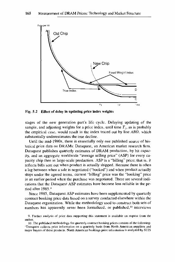
The most significant reason for this bias is probably the infrequent updating of the sample of products covered and recalibration of their relative weights. (Also, in recent years, fierce competition had led many U.S. producers to withdraw from producing certain of the products with the steepest price de- clines, so the slow decline of the BLS IC price indexes may also reflect in part a shift in the product mix of U.S. producers toward chips undergoing less rapid price declines.) Figure 5.2 sketches out a stylized view of the typical price trajectory over time for a new generation of memory chip-very steep initial declines, followed by much less rapid decline. Assume, for simplicity, that the mix of shipments quickly shifts to the new generation of chip when its cost per bit declines below that of the older generation chip, at time T , , but that very small quantities of the older generation chip are shipped for long periods afterward. An approximation to an exact price index would then look something like line ABC and would catch most of the rapid fall in the initial
165 Measurement of DRAM Prices: Technology and Market Structure
F per bit
C
\ idex
C
T i T2 Time
Fig. 5.2 Effect of delay in updating price index weights
stages of the new generation part’s life cycle. Delaying updating of the sample, and adjusting weights for a price index, until time T2, as is probably the empirical case, would result in the index traced out by line ABD, which substantially underestimates the true decline.
Until the mid-l980s, there is essentially only one published source of his- torical price data on DRAMS: Dataquest, an American market research firm. Dataquest publishes quarterly estimates of DRAM production, by bit capac- ity, and an aggregate worldwide “average selling price” (ASP) for every ca- pacity chip then in large-scale production. ASP is a “billing” price; that is, it reflects bills sent out when product is actually shipped. Because there is often a lag between when a sale is negotiated (“booked”) and when product actually ships under the agreed terms, current “billing” price was the “booking” price in an earlier period when the purchase was negotiated. There are several indi- cations that the Dataquest ASP estimates have become less reliable in the pe- riod after 1985.9
Since 1985, Dataquest ASP estimates have been supplemented by quarterly contract booking price data based on a survey conducted elsewhere within the Dataquest organization. While the methodology used to construct both sets of numbers has apparently never been formalized, or published,I0 interviews
9. Further analysis of price data supporting this statement is available on request from the author.
10. The published methodology for quarterly contract booking prices consists of the following: “Dataquest collects price information on a quarterly basis from North American suppliers and major buyers of these products. North American bookings price information is analyzed by SUIS

166 Kenneth Flamm
with various Dataquest staff members in 1989-90 provided some basic idea of the general procedures used at that time to construct these two series.
Prior to 1985, the Dataquest ASPS were apparently based exclusively on “informal inquiries” and “ongoing dialogue” on pricing trends with both pro- ducers and users of semiconductors. After 1985, when Dataquest began its quarterly survey of U. S. booking prices for semiconductor purchasing con- tracts, these quarterly U.S. booking prices have been the starting point for a more systematic estimation procedure for average selling (billing) prices worldwide. In essence, the estimation procedure applies considerable judg- mental input to survey data on U.S. booking (or order) price for a few standard parts, in order to derive a very much more detailed worldwide billing (or ship- ping) price matrix for a much larger number of products, which is then used to produce estimates of aggregate revenues, in turn the basis for the ASP esti- mates.” If the numbers fail consistency checks, or if customer feedback sug- gests that the numbers are inaccurate, or if significant doubts are otherwise raised, either the original booking price estimate based on survey data or the various pricing structure assumptions used to construct the ASPs, or both, is adjusted until “reconciliation” is accomplished. Thus, published Dataquest ASPS are a complex hybrid of limited survey data, analyst judgments, and informal dialogue with Dataquest’s customers.
The feedback from manufacturers and users may very well serve to improve these estimates of average quarterly billing prices. Comparable numbers are readily available within most chip producers’ sales and chip consumers’ pur- chasing departments. For this reason, the aggregate billing price estimates are probably more accurate than the quarterly booking price data, despite the fact that the latter, not the former, are what is actually measured in Dataquest sur- veys.
The quarterly price survey (of U.S. booking prices), apparently the only semiformal survey instrument used by Dataquest analysts in constructing their worldwide ASPs, is sent to approximately eighty to ninety U.S.-based com- panies, of which approximately 60 percent are manufacturers and 40 percent users. It covered 140 different types of parts in 1989 (of which a very small
[Semiconductor User Information Service] analysts for consistency and reconciliation. The infor- mation finally is rationalized with worldwide billings price data in association with product ana- lysts, resulting in the current forecast” (I thank Mark Giudice, of Dataquest, for providing me with this on 11 July 1990).
11. Conversation with Fred Jones, Dataquest Semiconductor Industry Service, 20 July 1990. The bookings price reported by the quarterly survey is “adjusted” to an equivalent billings price on the basis of an analyst’s estimate of the lag between bookings and billings, the effects of ongoing renegotiation of current (and write-downs of backlogged) orders under older contracts, and sales to the spot market. Estimates of product mix price differentials are then applied to a “base” billing price to get a price structure for a much larger number of products (other speeds, other organizations, other packaging) than is covered by the survey. Still more analyst estimates and judgments of regional price differentials are combined with detailed estimates of quantities shipped by region, then aggregated over regions, to arrive at a worldwide estimate of revenues and (after dividing by worldwide shipments) ASPs.

167 Measurement of DRAM Prices: Technology and Market Structure
number were DRAMS).’* Respondents are asked to provide estimates of their average booking price, for given products and volumes. The quarterly book- ing price estimate is then constructed as a weighted average of these re- sponses, with weights based on annual aggregate semiconductor production by responding producers and the estimated annual aggregate semiconductor procurement of surveyed consumers. Conceptually, therefore, it is neither an input, nor an output, nor a consumer price index. The survey covers only U.S .-based suppliers and purchasers.
Apparently in response to the creation of the “monitoring” system asso- ciated with the STA in 1986, price floors, and significant regional price differ- entials, Dataquest began a new program reporting regional contract pricing for a sample of twenty-five semiconductor components, on a biweekly basis. These data (the “Dataquest Monday Report”) are based on a survey of six to ten respondents, primarily chip manufacturers, in each of six geographic re- gions.I3 For DRAMs, the survey asks for the current contract price negotiated in three different volumes: 1,000, 10,000, and volume (over 100,000).14 If producers have not concluded any contracts for a particular volume, they are asked to estimate the price that would have been negotiated on a contract of that size. Japanese producers do not report a contract price, and Japanese price data refer to “large volume wholesale” prices.
The data discussed thus far have largely ignored DRAMs sold by distribu- tors and in the spot market. This misses an important dimension of the change in market conditions after the signing of the STA. To remedy this situation, I have constructed time series showing retail spot prices for memory chips, be- ginning in the spring of 1985. To do so, I collected weekly data on sales prices by one of the largest retail vendors of memory chips in the United States.15 The advertised prices are dated (an important point since there is typically a substantial lag between the submission of advertising copy and its publica- tion). Contacts with this vendor have also made it clear to me that these are real prices; that is, in-stock product is actually available at these prices. The contrast with contract prices is striking: spot retail prices for 256K DRAMs quadrupled between early 1987 and early 1988, while U.S. contract prices (as measured by the Dataquest Monday series) merely increased by 60 percent!
The conclusion that emerges from a comparison of the bits and pieces of information available on DRAM pricing is that, prior to 1985, various avail- able price series are roughly consistent and tend to move relatively closely together. Significant regional differentials were not important. All this changed after 1987; it became much more important to disaggregate by sales
12. By the spring of 1990, the survey had been expanded to cover 21 1 types of parts. 13. I thank Mark Giudice, of Dataquest, who, in various conversations in 1989 and 1990,
provided the description of the Dataquest Monday Report Survey given here. 14. In some published Dataquest reports, it is stated that “volume” prices mean greater than
20,000 parts, not 100,ooO; the definition of volume for DRAMs is apparently an exception to this rule.
15. A detailed analysis of these data may be found in Flamm ( 1993).
168 Kenneth Flamm
channel and region in tracking DRAM prices actually faced by users. For example, assume that the grey market accounted for 15 percent of consump- tion by volume and 25 percent of consumption by value in some base year. If grey market sales prices quadruple (to construct a not-so-hypothetical ex- ample) while prices in other sales channels merely double, the increased cost to chip consumers will be about 25 percent greater than what is shown by a price index based solely on sales through non-grey market channels!
5.4 The Economic Role of Contract Pricing
Given that perhaps 70 percent of DRAM sales are initially made as direct “contract” sales to large users, it is useful to examine the nature of these con- tracts in detail. An econometric analysis of contract prices will permit one to control for detailed characteristics of DRAMs and DRAM contracts and more accurately measure a “quality-adjusted” price for DRAMs. The analysis will be applied in constructing Fisher Ideal price indexes in the next section of this paper.
Typically, “contract” sales are commitments to supply some quantity of parts, at some specified price, beginning at one future date, and ending at another future date. However, they rarely seem to be legally binding commit- ments. The prices specified in these long-term contracts generally appear to hold when shipments under the contract begin but often do not persist over the life of the contract. Many contracts contain explicit provisions for renegotia- tion of price downward, at the purchaser’s option, in response to changing market conditions; purchasers also successfully demand downward price ad- justments even when no such provision is explicitly made.16
Furthermore, because the system of price floors for DRAMs put into place by the U.S. Commerce Department in 1986 specified that the prevailing floor price at the time a legally binding contract was drawn up and signed remained in force throughout the life of the contract, despite expected future declines in DRAM prices, there was an additional disincentive to producing a formal, legally binding document. On the other hand, suppliers generally seem to respect contract prices as a de facto ceiling on prices charged their customers (although, during the unprecedented increase in memory chip prices of 1987- 88, some purchasers apparently did face cancellation or reduction of pre- scribed contract volumes at the negotiated price).
If contract prices are generally not legally or practically binding much be- yond the original beginning date for the contract, what then is the purpose of entering into one of these informal, “handshake” commitments? Interviews with OEM purchasing managers suggest that assuring the quantity of DRAMs
16. An interesting compendium of DRAM contract “horror” stones-users and producers re- pudiating oral and written price commitments in response to changing market conditions-may be found in USITC (1986, A-75-A-82).
169 Measurement of DRAM Prices: Technology and Market Structure
to be purchased from suppliers is the major objective of these arrangements. In fact, purchasers frequently suggest that the critical issue in times of extreme shortage is not necessarily pricing but getting adequate supplies. Spot market purchases may create other significant costs for the chip consumer that extend beyond the purchase price. Additional qualification costs or extensive addi- tional testing may be required for purchases from new sources or grey market suppliers.
Producers of DRAMs face a different logic. Significant “learning-curve’’ effects lead to a sharp increase in the output of any given initial investment in DRAM production capacity over the product life cycle of that generation of DRAM. Producers must be concerned about volatility in demand for the in- creasing quantities of DRAMs that will be flowing off of existing fabrication lines in future periods. Quantity commitments lock purchasers into deliveries of a given producer’s output and reduce the odds that large volumes of chips emerging from ever more productive factories will have to be liquidated in the grey market.
My working hypothesis, then, is that long-term chip contracts represent the marriage of quantity commitments to a forward price in force at the beginning of the contract. Over the remaining life of the contract, however, contract buyers seem to enjoy something like the “price protection” offered to distrib- utors.
5.4.1 Econometric Analysis of Contract Pricing I collected confidential data on OEM DRAM contracts covering the period
1985-89 from industry sources. The data are drawn from contracts negotiated by a small number of European and North American electronic equipment OEMs; the bulk of the reported contracts refer to purchases by European users. Characteristics of the contracts that were collected include negotiation date, start date for shipments, period over which shipments are to be deliv- ered, total quantity commitments over this period, contract price, nationalities of chip vendors (American, European, Korean, and Japanese) and purchasers, chip organization and packaging, and chip speed (access time). After discard- ing contracts for which speed measures were unavailable (or covering parts with a mixture of speeds), parts that used packages other than plastic dual in- line pin (DIP), plastic-leaded chip carrier (PLCC, in the case of 256K DRAMs only) and small outline cases (SO, in the case of 1M DRAMs only),” and chips with relatively uncommon organization,I8 a sample of 83 agree- ments for 64K DRAMs, 174 for 256K DRAMs, and 128 for 1M DRAMs remained. A growing variety of chip organizations and packaging in this
17. These involved a small number of observations divided among a relatively large group of other packages. Only 256K DRAMs with access times of 120 ns, or faster, were packaged in PLCC cases in the contracts in this sample.
18. Chip organizations other than 64K X 1, 256K X 1, 1M X 1, or 256K X 4 (the latter two are 1M DRAM types) appeared only in a relatively small number of contracts in my sample.

170 Kenneth Flarnrn
sample, with each new generation of DRAM, confirms my earlier observa- tions about increasing product differentiation in the DRAM market.
I examined the distribution of these contracts by lead time (months from negotiation date to start date) and length (duration of contract, months from start date to end date). It was readily apparent that the vast bulk of these con- tracts begin with a very short period after their negotiation. The contract lengths cluster around three-, six-, and twelve-months’ duration. More than 40 percent of the contracts for 64K and 256K DRAMS and 29 percent of those for 1M DRAMs could be considered “spot”: shipments were scheduled to begin in the month they were negotiated. A large but smaller fraction (38 percent of the lM, 28 percent of the 256K, 14 percent of the 64K) were to begin in the month following the contract’s negotiation. All remaining con- tracts began within two to six months for 64K parts; 2 percent of 256K DRAM and 7 percent of 1M DRAM contracts began more than six months later.
The distributions for 64K and 256K DRAM agreements before and after September 1986 suggest that contracts negotiated after that date tended to have longer lead times and to last longer. A formal chi-square test comparing pre- and post-STA distributions generally confirmed these casual impres- sions.I9 (But note that the period prior to the signing of the STA was one in which markets saw abundant supplies and generally declining prices, while 1987 and 1988 were generally marked by firm or rising prices and tightening supplies.)
My analysis treats observed prices as being derived from some “base” mar- ket price for a standard DRAM in a plastic DIP case, corrected for the incre- mental costs of more complex packaging (recall the discussion of “packaging arbitrage” above). Discussions with electronics purchasing personnel suggest that this is, indeed, how price is conceptualized when contracts are negotiated (i.e., projections of the prevailing prices for the “base” product are added to the cost of specialized packaging). Quantity discounts (presumably reflecting fixed selling costs) and vendor nationality effects (which may reflect percep- tions of quality by chip consumers or distinctive sales strategies by groups of firms) will also be considered as possible reasons for deviation from prevail- ing “base” DRAM prices. Prices paid by European and American customers will also be permitted to differ in the statistical analysis, in order to test for the apparently increasing regional segmentation of DRAM markets after 1986. Specification of the determinants of this “base” price is the subject to which I next turn.
5.4.2 An Econometric Model of Forward Pricing in DRAMs My starting point is the notion that these “contract” prices are forward
prices, reflecting expectations at the negotiation date for spot DRAM prices at
19. Rejecting a null hypothesis of no change at the 5 percent level, 1 conclude that both lead times and lengths of contracts signed for the newer 256K DRAMs seem to have increased after the STA was signed, while lead times increased for more mature 64K chips (but I did not reject the hypothesis of no change in the distribution of lengths).

171 Measurement of DRAM Prices: Technology and Market Structure
the start date for the contract. The 40 percent of contracts that start immedi- ately are true “spot” prices. If these contract prices were truly binding over the life of the contract, then one would further expect this price to decline with contract length, in a regime of falling DRAM prices, since the fixed price would have to be adjusted down to leave a purchaser indifferent between a longer contract and a sequence of shorter-term forward contracts. (The oppo- site, of course, would occur in a regime of rising DRAM prices.) Length of contract has been included as an explanatory variable in order to test the null hypothesis that contract length plays no significant role in price determina- tion, in accordance with the a priori perception that initial contract price is generally renegotiated as soon as there are significant reductions in DRAM prices.
My approach is borrowed from the literature on futures prices.*O The basic identity is
wheref: is forward price at time r for period s, Er[PS] is the expectation- conditional on information available at time r-of spot price in period s, and 5: is defined as bias, the difference between forward price and expected spot price.
If the forward price is “unbiased,” then the 5 term will be zero. On the other hand, a risk-averse speculator requires a positive return to buy forward con- tracts and accept the risk associated with uncertainty about future prices, so the 5 term may be negative. The latter situation was described by Keynes as his theory of “normal backwardation.” Whether future prices generally are unbiased, or exhibit normal backwardation, or possibly even a positive bias, is the subject of heated debate and will be treated as an empirical question in what follows.2’
At a minimum, I shall assume that, for any generation of chip, market par- ticipants’ expectations about supply and demand fluctuations are generated by some “model” that remains constant over the product life cycle of that chip and that a fixed stationary term structure of forward contract prices prevails, that is, that the bias term in equation (1) is given by a function of delivery lead time, s - r (aside from random, mean zero disturbances). This means that we can rewrite ( 1 ) as
Deviations of forward prices from expected spot price at delivery are given by a set of constants, with exactly one corresponding to each possible value of lead time to delivery.
20. The primary distinction between a futures price and a forward price is that the futures market is relatively large and well organized, with a high degree of standardization of contracts and commodities, well-refined tools and procedures to make contracts legally enforceable, and government regulation of trading behavior.
21. For a spectrum of different approaches to this issue, see Chari and Jagannathan (1990), Stein (1987, chaps. 1, 2), Newbery (1987), Houthakker (1987). and Williams (1986).

172 Kenneth Flamm
As an alternative approach to specification, we start with Stein’s model of futures markets (see Stein 1987, chap. 2). Bias is proportional to the condi- tional (at time r ) variance of spot price at delivery time s, V,[P,]:
(3 )
with h representing net hedging pressure (the excess supply of forward con- tracts were forward price set equal to the expected future spot price), and u a function of such market characteristics as degree of risk aversion and relative numbers and types of different classes of market participants.** The latter can reasonably be taken as relatively constant; the behavior of net hedging (as measured empirically in traditional commodities future markets) has also not been particularly volatile (Stein 1987, 63). In what follows, I assume that, over the relatively short time periods examined in this paper, the hedging pres- sure h can be taken as randomly varying around some fixed mean H , that is,
(4) h, = H + q,, with the q, i.i.d., mean zero random disturbances.
If we then take the additional step of assuming that conditional variance V,[P,] is approximately proportionalz3 to s - r, lead time (with constant of proportionality a*), we then have
with b = - H u ~ / u . ~ ~ If forward prices are unbiased, b is zero; if they exhibit normal backwarda-
tion, b is negative. This specification effectively imposes a series of linear constraints on the less restrictive specification of a fixed, stationary term structure of forward contract prices set out in equation (2), that is, that <(s - r ) = b(s - r ) , and can therefore be tested.25
To actually estimate (3, we may add on a mean zero random disturbance term, vr, and (incorporating [4]) rewrite it as
22. Other approaches to modeling futures prices can also yield a bias in forward price propor- tional to the conditional variance of price (see Newbery and Stiglitz 1981, chap. 13; and Newbery 1987,445).
23. Because V,[P,] must equal zero, I have constrained the intercept of a linear approximation to equal zero.
24. Or, with a deterministic supply and price given by adding permanent random shocks onto a deterministic inverse demand function, a conditional variance V,[P,] proportional to s - r can be explicitly derived.
25. That is, if the coefficient of the lead time dummy variable for a contract with a two-month lead time is constrained to equal two times the coefficient of the dummy variable for a contract with a one-month lead time, the coefficient of the dummy variable for a three-month lead time is constrained to equal three times the coefficient of the dummy variable for a contract with a one- month lead time, etc., we produce specification (5).

173 Measurement of DRAM Prices: Technology and Market Structure
Assuming rational expectations, the expression in braces will on average equal zero, and we might wish to incorporate it, and all terms to its right, into a random disturbance term and not explicitly model the formation of expec- tations. However, the difference between conditional expectations and their future realization (the expression in braces in [6]), which becomes part of the error term in a regression equation, will generally be correlated with P, and therefore calls for more complex estimation strategies. My approach will be to use instrumental variables. Note as well that the random disturbance term in (6) is explicitly heteroskedastic.
I do not actually have data on spot prices for large user contracts; however, I did construct the time-series data on spot retail prices in the United States described earlier. Large-volume U.S. spot contract prices were assumed to be related to U. S, retail spot prices by the relation
(7) Ps = c + dRs,
where R, is retail spot price at time s. The presumed constancy of this relation in the U.S. market can be used to identify changes in price differentials be- tween U.S. and European markets, with the use of appropriate dummy vari- ables (i.e., shifts in parameter c), even if no U.S. contract data are actually available, in a sample composed exclusively of European contracts. If any U.S. contracts are available in the sample, actual differentials (distinct levels for the United States and Europe), as well as changes over time, are identified when (7) is substituted into (6) . Thus, even if data on U.S. contract data are unavailable over periods when price differentials between the United States and Europe are believed to have changed, we can still check for such changes by regressing European contract prices on U. S. retail spot prices.
Finally, note that the semiconductor industry habitually analyzes its prices on diagrams with logarithmic scales. I shall regard contract prices, and mod- els of pricing, as being set and analyzed in the logs of prices and will under- take the econometric analysis of chip prices using logarithmic functional forms. In equations (1)-(7), then,f, and R should be read as the logarithms of the respective prices; the analysis is otherwise unchanged.
5.4.3 Estimation The model to be estimated, which relates forward prices, by delivery date,
to actual spot prices on that delivery date, assumes DRAM base price is de- scribed by (7) and (6) , modified to take into account possible economies of scale in purchasing, costs of special packaging, and possible price differen- tials specific to producer and consumer geographic region. This specification is given by

174 Kenneth Flamm
with u a statistical disturbance term, and Q purchase volume in thousand units. “Package” is a dummy variable for specialty packaging (PLCC for 256K DRAMs, small outline for 1M DRAMs); “ven” are dummy variables that denote Korean, European, and American vendors (expressing price dif- ferentials as deviations from the price quoted by a Japanese vendor); and “eurt” are dummy variables introduced to measure differentials in prices paid by European consumers (relative to the North American market) over discrete periods of time. Retail spot prices lagged n periods and earlier were used to instrument Rs, with n chosen to exceed the maximum lead time (s - r ) before a contract began in the actual sample (to ensure that all instruments precede Rr and can reasonably be regarded as predetermined).
Because the retail spot price series were constructed for only a single speed of DRAM for each density of chip, and because earlier analysis suggested that price changes over time varied substantially by speed of chip for any given density, analysis was restricted to those contracts for which U.S. retail spot price data relating to the appropriate speed had been constructed. Results are organized and discussed by chip density.
256K DRAMs
Because time-series data were constructed only for retail spot prices for 120 ns, 256K x 1 DRAMs (extended back to 1984 by linking to the International Trade Commission spot 256K DRAM price data), a subset of eighty-seven contracts covering 120 ns DRAMs, in DIP and PLCC packages, was used to estimate equation (8). The limited availability of historical time-series data on monthly spot prices meant that sample size was maximized by further restrict- ing the exercise to contracts with lead times of up to four months (two obser- vations with seven-month lead times were eliminated from the sample as a result), leaving eighty-five observations in the sample. Seventy-nine of the contracts were with European customers and six with American chip consum- ers. Six contracts were with Korean vendors, six with European producers, twenty-two with American firms, and the balance with Japanese companies.
Coefficient estimates and asymptotic standard errors are shown in table 5.1. Only instrumental variable estimates are shown, but OLS parameter estimates were in all cases quite close to the instrumental variables estimates. Available data permitted the use of prices lagged from five to eight months prior to the contract start date (since the maximum contract lead time was four months) as instruments.
Examination of the Dataquest regional contract price estimates led me to use four dummy variables to capture European price differentials prevailing at different contract start dates: EUR, a base Europe-U.S. differential dummy

175 Measurement of DRAM Prices: Technology and Market Structure
Table 5.1 Econometric Analysis of 256K DRAM Contracts (two-stage least squares regression)
With Contract Length Without Contract Length Variable Variable
Dependent variable Mean of dep. var. SE of regression No. of observations SD of dep. var. Sum of sqrd. residuals
LogPRICE 1.047 0.205 85 0.326 3.575
LogPRICE 1.047 0.205 85 0.326 3.575
Constant LogQUAN LENGTH LEAD PLCC LogSPOT Vendor dummies:
EURVEN KORVEN USVEN
EUR ETA ETB ETC
Time-period dummies:
~~~
Results Corrected for Heteroskedasticity
Coeff. SE CWff. SE
0.917 0.208* 0.921 0.204* -0.0376 0.0237 - 0.0374 0.0235
0.000470 0.00624 . . . . . . -0.0364 0.0210*** - 0.0363 0.0207***
0.103 0.0409** 0.104 0.0390* 0.282 0.0737* 0.282 0.0717*
- 0.0732 0.0514 -0.0738 0.0525 0.0791 0.0561 0.0791 0.0559 0.0139 0.0806 0.0138 0.0804
- 0.147 0.121 - 0.148 0.118 -0.118 0.0704*** -0.116 0.0721
0.001 16 0.0783 0.00268 0.0815 0.170 0.135 0.171 0.135
HO: No Europe4J.S. price differentials: Wald statistic,
x2(4) = .2208
*Reject hypothesis of equality with zero, two-tailed test, I percent significance level. **Reject hypothesis of equality with zero, two-tailed test, 5 percent significance level.
***Reject hypothesis of equality with zero, two-tailed test, 10 percent significance level.
variable with a value of one for European contracts throughout the sample period (August 1985-January 1989), zero elsewhere; ETA, a dummy variable with a value of one for European customers during period A (September 1986-February 1987, the beginning of the STA through the end of a period when Dataquest shows European prices somewhat lower than U.S. prices), zero in all other cases; ETB, equal to one for European contracts starting over March 1987-June 1988 (where the Dataquest data show European and Amer- ican prices moving more or less together), zero elsewhere; and ETC, equal to one when European customers’ contracts started during period C (July 1988-

176 Kenneth Flamm
April 1989, when Dataquest showed European prices significantly higher than U.S. prices), zero elsewhere.
An initial specification test did not lead me to reject the null hypothesis of linearity in lead time (although not shown, a version of the model correspond- ing to equation [2]-with an unrestricted term structure, using individual monthly lead time dummies-was first estimated).26 Because heteroskedastic disturbance terms are a distinct possibility (individual contract sizes ranged from five thousand to 8.9 million chips), heteroskedasticity-consistent stan- dard errors were calculated.
The coefficient of contract length was quite small and statistically indistin- guishable from zero at any reasonable significance level. (Two-tailed tests of significance were used for all coefficients.) The second half of table 5.1 shows the resulting estimates when this hypothesis is maintained; the coefficient es- timates show virtually no change.
The coefficient of lead time was negative (suggesting bias in the forward price) and statistically significant at the 10 percent level but not at the 5 per- cent level, with forward price declining 3.6 percent with every additional month of lead time before delivery. None of the European price differential dummies were statistically distinguishable from zero at these significance lev- els. Indeed, the point estimates of European price differentials were generally negative, except in period C, and most negative in period A, right after the signing of the STA. The grossly higher European 256K DRAM prices shown by Dataquest data from July 1988 through early 1989 contrast with a much smaller estimate of this differential (about 2 percent higher in Europe) within my sample of contracts. A Wald test for the hypothesis that there were no price differentials between the United States and Europe, before and after the STA, does not permit us to reject this c ~ n j e c t u r e . ~ ~
Quantity discounts do not seem to be a significant factor. The statistically insignificant coefficient for units to be shipped suggests that increasing con- tract volume tenfold produces a roughly 8 percent decline in unit price, a modest discount. I interpret this to mean, not that purchase volume is irrele- vant to pricing, but that the relatively large companies in my sample get the benefit of the largest volume discounts based on their overall status as a vol- ume account, not on the details of individual contract transactions. Plastic- leaded chip carrier (PLCC) packaging is associated with a statistically signif- icant premium.
My point estimates indicate that Korean producers seem to have charged 8 percent more for their 256K DRAMS than Japanese vendors over the entire period, but the estimated standard error is quite large, and the hypothesis of
26. The Wald statistic was .0654, with three degrees of freedom; the null hypothesis cannot be
27. The Wald statistic, with four degrees of freedom, was .221; the null hypothesis cannot be rejected at any reasonable significance level.
rejected at any reasonable significance level.
177 Measurement of DRAM Prices: Technology and Market Structure
no difference in pricing cannot be rejected at the 5 percent level. American and European producers also show pricing differences with Japanese compet- itors that are statistically insignificant at this level.
1M DRAMs
For 1M DRAMs, the retail spot price time series that I have constructed covers 1M X 1 chips with 100 ns access times, in DIP packages, and extends back to June 1986. Available contract data for these chips in either DIP or small outline (SO) packages covered sixty-two observations, with the first two beginning in July 1986 and another eight negotiated before June 1987. Sample size was maximized by dropping these ten observations and including only the subset of fifty-two contracts with lead times under eight months; the first con- tract in this reduced sample started in June 1987, after the STA had been signed.
Results appear in table 5.2 and are basically similar to those for 256K parts; heteroskedasticity-consistent standard errors were again calculated.28 Exami- nation of the Dataquest regional contract price estimates led me again to con- struct four dummy variables to capture European price differentials for 1M DRAMs at different contract start dates. First, a base Europe-U.S. dummy variable for the entire sample period (June 1987-January 1989) was con- structed. Over most of this post-STA epoch, Dataquest showed European and American 1M DRAM prices moving more or less together. Other periods, when regional price differentials seem to show up in the Dataquest data, were accounted for by constructing additional dummy variables: these included pe- riod A, June 1987-July 1987 (fragmentary Dataquest data show European prices somewhat lower than U.S. prices at the beginning of this period); pe- riod B, November 1987-January 1988 (where the Dataquest data again show European prices falling below American prices); and period C, April 1988- October 1988 (when Dataquest showed European prices significantly higher than U. S. prices).
The European price differential dummies for the entire sample period and period A were relatively large, negative, and statistically significant at both the 5 and the I percent levels, while the dummy for period B was small and statistically insignificant. The dummy for period C was positive and statisti- cally significant (at the 5 or 1 percent levels) but would imply that European prices were slightly lower over this period. Thus, if one were to accept the notion of regional price differentials, European 1M prices generally appear to
28. As before, only instrumental variable estimates are shown; OLS parameter estimates were in all cases relatively close to the instrumental variables estimates. Available data permitted the use of prices lagged from eight to eleven months prior to the contract start date as instruments. Eleven of the contracts were with American customers, forty-one with European customers. Four of the contracts were with Korean chip producers, three with American companies, three with European vendors, and the balance were Japanese. Once more, an initial specification did not lead to rejection of the null hypothesis of linearity in lead time, at the 5 percent significance level. The Wald statistic was .100, with six degrees of freedom.

178 Kenneth Flamm
Table 5.2 Econometric Analysis of 1M DRAM Contracts (two-stage least squares regression)
With Contract Length Without Contract Length Variable Variable
Dependent variable LogPRICE LogPRICE Mean of dep. var. 2.861 2.861 SE of regression 0.0838 0.0860 No. of observations 52 52 SD of dep. var. 0.144 0.144 Sum of sqrd. residuals 0.365 0.385
Results Corrected for Heteroskedasticity
Coeff. SE CWff. SE
Constant 2.378 0.377* 2.431 0.343* LogQUAN -0.0209 0.0165 - 0.0213 0.0165 LENGTH -0.00724 0.00353** . . . . . . LEAD - 0.01 10 0.00609*** -0.0110 0.00584** * SOJ 0.0270 0.0324 0.0345 0.0325 LogSPOT 0.219 0.109** 0.188 0.0997*** Vendor dummies:
EURVEN -0.0127 0.0366 -0.0162 0.0385 KORVEN 0.108 0.0521** 0.106 0.0507** USVEN 0.0363 0.0243 0.0512 0.0258**
ESTA -0.156 0.0482* - 0.145 0.0485* ETA -0.187 0.0545* -0.219 0.0506* ETB 0.00532 0.0375 -0.0133 0.0404 ETC 0.0946 0.0359* 0.103 0.0325*
Time-period dummies:
HO: No Europe-U.S. price dif- ferentials: Wald statistic,
x2(4) = ,3036
*Reject hypothesis of equality with zero, two-tailed test, 1 percent significance level. **Reject hypothesis of equality with zero, two-tailed test, 5 percent significance level.
***Reject hypothesis of equality with zero, two-tailed test, 10 percent significance level.
have been somewhat lower than those in the United States and very much lower in the summer of 1987. Using a joint test statistic, however, the hypoth- esis that there were no price differentials throughout the sample period could not be rejected.29
64K DRAMS
For 64K DRAMs, the retail spot price time series that I created covers 64 x 1 chips with 150 ns access times, in DIP packages, goes back to May
29. The Wald statistic (four degrees of freedom) was ,304; one cannot reject at any reasonable significance level.
179 Measurement of DRAM Prices: Technology and Market Structure
1985, and ends in mid-1987. This series was extended back to February 1982 by linking to data tabulated by the International Trade Commission (ITC) in the course of an antidumping investigation; it was extended forward to 1989 by linking to a wholesale price series based on data found in Nihon Keizai Shimbun, converted into dollars at prevailing exchange rates.3o (I judge this composite index to be a significantly less accurate indicator of movements in the U.S. retail spot market than the series used for 1M and 256K DRAMs, and this caveat should be borne in mind when interpreting my results.) Avail- able data for these chips in DIP packages covered fifty-one contracts, with the first one beginning in April 1985 and the last in February 1989. Maximum lead time was six months, so I was able to use all observations in this sample. Forty-four of the purchasers were European companies, the balance Ameri- can. Two of the contracts involved vendors who were Korean, three were with European producers, eleven dealt with American firms, and the balance were with Japanese companies.
Results are displayed in table 5.3 and again, are basically similar to those for 256K DRAMS.~] Available data permitted the use of prices lagged from seven to ten months prior to the contract start date as instruments. Since no Dataquest regional contract price estimates are available for 64K DRAMs, the same four dummy variables used to capture European price differentials for 256K DRAMs at different contract start dates were used for 64K DRAMs.
All four European price differential dummies were statistically significant at the 10 percent level, and two were statistically significant at the 1 percent level. The pattern of differentials associated with these estimates is of Euro- pean 64K DRAM prices falling almost 20 percent lower than U.S. prices prior to the signing of the STA, then gradually rising to a level almost 20 percent greater by early 1989.
Summary
An econometric analysis of DRAM contract price data for three successive generations of memory chips has supported several general propositions. First, the simple model of the term structure of forward prices that I am using seems quite consistent with these data: formal statistical tests did not reject it, and estimated coefficients were largely unaffected by imposition of this set of constraints. Second, my a priori suggestion that, beyond the initial purchase at the contracted price, these contracts mainly represent quantity commit- ments is supported by the generally small magnitudes and statistical insig-
30. Quarterly ITC data for spot-market sales of 64K DRAMs in quantities of under 10,OOO chips were imputed to the middle month of every quarter, and data for the remaining months of each quarter were produced by interpolation between these mid-quarter observations. Because my retail spot price series began in May 1985, only a small number of observations relied on these interpolated ITC data.
3 1. As before, an initial specification test leads one not to reject the null hypothesis of linearity in lead time, at any reasonable significance level. The Wald statistic was ,389, with five degrees of freedom, Heteroskedasticity-consistent standard errors were again calculated.

180 Kenneth Flamm
Table 5.3 Econometric Analysis of 64K DRAM Contracts (two-stage least squares regression)
With Contract Length Without Contract Length Variable Variable
Dependent variable Mean of dep. var. SE of regression No. of observations SD of dep. var. Sum of sqrd. residuals
LogPRICE -0.0191
0.177 51 0.368 1.604
LogPRICE -0.0191
0.178
0.368 1.610
51
Results Corrected for Heteroskedasticity
COeff. SE Coeff. SE
Constant LogQUAN LENGTH LEAD LogSPOT Vendor dummies:
EURVEN KORVEN USVEN
EUR ETA ETB ETC
Time-period dummies:
-0.241 -0.0156
0.00669 - 0.0644
1.248
0.0343 0.313
-0.0196
-0.205 0.245 0.307 0.449
0.153 0.0221 0.00827 0.0185* 0.449*
0.104 0.136** 0.0722
0.0868** 0.0698* 0.0954* 0.225* *
0.232 0.152 -0.0113 0.0206
- 0.067 1 0.0183* 1.359 0.398*
0.0466 0.106 0.332 0.134**
- 0.0293 0.0688
-0.201 0.0868** 0.256 0.067 1 * 0.294 0.095 1 * 0.390 0.208***
HO: No Europe-U.S. price differentials: Wald statistic,
~ ~ ( 4 ) = .5392
*Reject hypothesis of equality with zero, two-tailed test, 1 percent significance level. **Reject hypothesis of equality with zero, two-tailed test, 5 percent significance level.
***Reject hypothesis of equality with zero, two-tailed test, 10 percent significance level.
nificance of the coefficients of contract length as a determinant of contract pricing.
Analysis of price differentials faced by American and European purchasers of DRAMS suggested much smaller differentials than had been indicated by the Dataquest Monday contract price data, and, overall, I could not reject the null hypothesis of no regional differences. The sign of point estimates of these differentials was generally consistent with the pattern suggested by Data- quest’s numbers, however.
The general pattern that emerged of Korean vendors, selling their product at somewhat higher prices is consistent with anecdotal observations by market

181 Measurement of DRAM Prices: Technology and Market Structure
participant^.^^ It suggests that Korean producers were following an opportun- istic pricing strategy focused on short-run rent extraction in marginal demand not covered by long-term contracts with other producers, rather than the es- tablishment of long-term relationships with a stable set of customers. In ef- fect, in a period of scarcity, the Korean producers may have charged a higher price than the long-term contract price, approaching the spot grey market price, while, in a period of glut, the Koreans would charge a lower price, again approaching the spot grey market price. Since Korean product in my sample was shipped only during periods of relatively tight markets (i.e., after 1986, through early 1989), this would explain the positive differential on con- tracts for Korean product. This analysis is also consistent with the reports in the trade press on Korean producer Samsung’s dealing with its American dis- tributors. B3
In my model, the coefficient of lead time measures the “bias” in forward prices. My empirical results supported the presence of “normal backwarda- tion” in forward contract prices for DRAMs. My point of departure was a model in which bias in forward prices serves to compensate purchasers for the transfer of risk to them by producers. The rather dramatic decline of the bias term from the 64K generation of DRAMs, to the 256K generation, to the 1M generation, suggests that the market viewed prices for current generation chips as considerably less volatile than previous generations of chips. This, of course, was precisely what the administrative pricing guidelines and mecha- nisms imposed on the DRAM market with the advent of the STA would have been expected to accomplish.
5.5 Improved Price Indexes for DRAMs
The econometric results presented above can be used to address several of the many problems in existing data on DRAM prices surveyed earlier. Leav- ing aside data and sampling issues, those problems can be grouped into two distinct categories: problems related to product heterogeneity and problems related to the aggregation of prices over time.
This first problem is the variety of products and distribution channels. While at one time DRAMs of given density were a relatively homogeneous product, the proliferation of organizations, packaging, and speeds has meant
32. One Korean producer-Samsung-was responsible for the vast majority of Korean DRAM sales over the period covered in this sample.
33. At the peak of the DRAM shortage, in the summer of 1988, Samsung attempted to hike its prices to levels that its American distributors protested left them uncompetitive and temporarily ended price protection for distributors (see Elecfronic News, 15 August 1988, 47; 27 February 1989, 27; 3 April 1989, 35). When prices turned down sharply in early 1990, Samsung shocked its American distributors by doing away with the customary “price protection” altogether. Ameri- can distributors complained bitterly about Samsung’s “broker mentality” (see Elecrronic News, 22 January 1990,34; 5 February 1990,38; 2 July 1990,32).

182 Kenneth Flamm
that the volume-weighted averages published by industry sources now aggre- gate over a large variety of different parts, so that changes in product mix within a sample-as well as transaction size if there are quantity discounts- may produce significant changes in average prices. The existence of multiple distribution channels-larger user volume contracts, authorized distributors, and grey market brokers-means that shifts among distribution channels may also affect average prices in unpredictable ways.
The second complication stems from the fact that chip sales are often embedded in forward contracts, so we can associate a chip sales price with both negotiation and delivery dates. From the standpoint of measuring com- pany revenues or a producer price index, for example, one might choose to measure average sales or billing prices, the actual average price received per chip shipped in a given period. These are essentially shipment-weighted av- erages of prices on contracts booked both in the past (subject to some revision) and in the current period.
However, for an economist interested in the cost of chips as an input to the production of other products, it may be useful to have some notion of current market cost, at the margin, of additional supplies of that input. The current “average” booking price will not do; it is actually a weighted average of the current market price for spot contract deliveries and expected market prices in future periods when deliveries on contracts with future delivery dates will begin, further complicated by the possible existence of discounts in pricing for future delivery due to “normal backwardation.” An ideal measure of cur- rent input cost arguably would measure the price of the input for immediate delivery only (with booking price equal to billing price) since this is the true opportunity cost relevant to a consumer of the product at the moment of use.
I turn next to the construction of price indexes that address both sets of concerns, using the empirical results of the preceding section. Since virtually all the technological improvements in DRAMS-in the form of greater den- sity, novel organizations, smaller power consumption, and faster speeds- have been embodied in the introduction of distinctive new product types, deal- ing in a satisfactory way with the effect of product differentiation is equivalent to constructing a quality-adjusted price index for DRAMs.
5.5.1 The first step was to calculate the average sales price for as many distinct
types of DRAMs as possible, for which contract data were available in relative abundance (so a reasonable approximation to a time series could be con- structed). For 1M and 256K DRAMs, this meant using data for ‘‘x 1” orga- nized chip types of two speeds and “ x 4” organized chip types of one speed, in DIP, SO, and PLCC packages. For 64K DRAMs, this meant using data on “ X 1” organized DRAMs of two distinct speeds, in DIP packages. Alto- gether, 116 contracts for 1M chips, 196 contracts for 256K chips, and 71
Construction of Average Billing Prices

183 Measurement of DRAM Prices: Technology and Market Structure
contracts for 64K chips were used to construct quarterly price indexes span- ning the period from the second quarter of 1985 to the first quarter of 1989.34
In constructing my price indexes, two adjustments were made to the origi- nal data, to control for variance in price attributable to quantity and packag- ing. All prices were adjusted to a quantity 100,000 basis, using the estimated coefficients reported in the empirical results above. (Although the estimated coefficients for quantity discounts were small and had relatively large standard errors, a priori knowledge suggests the existence of some discount.) These coefficients were assumed to apply to all chips of the same density, including those with speeds and organizations different from those used for the econo- metric analysis. (A 256K X 4, 100 ns 1M DRAM, e.g., was assumed to face the same quantity discount structure as a 1M X I , 120 ns DRAM.) Also, chips packaged in PLCC and SO cases were adjusted to a DIP package basis using the coefficients estimated
It was further assumed that product shipped under a contract was delivered at the start of the contract at the negotiated price. (Renegotiation of price was assumed to affect only deliveries after this initial delivery.) Thus, for every contract, the negotiated price was attributed to the quarter in which product was first shipped. Individual contract prices were weighted using total con- tract quantity divided by the length of the contract (an estimate of average monthly delivery volume under the contract), to produce a weighted average quarterly shipment price for each type of chip.36 The products of these average prices (after “adjustment” to a quantity 100,000, DIP package basis) and their quantity weights were then used to produce estimates of total (adjusted) ex- penditure shares on chips of various types within this sample.
Table 5.4 shows how rapidly the distribution of (adjusted) expenditure shifted historically within the sample, as new types of chips were brought to market. The extraordinary speed with which these expenditure shares shift
34. For 1M DRAMs in DIP or SO packages, 62 observations on 100 ns 1M x 1 parts (52 of which had been used in the econometric analysis of the last section), 26 observations on 120 ns 1M x 1 parts, and 28 observations on 120 ns 256K x 4 chips were used. For 256K DRAMs in DIP or PLCC packages, there were 87 observations on 120 ns 256K X 1 chips (85 of these observations had been used in our econometric sample), 75 contracts for 150 ns 256K x 1 chips, and 34 observations for 120 ns 64K X 4 parts. For 64K DRAMs in DIP packages only, there were 51 observations on 150 ns 64K x 1 chips and 21 contracts for 120 ns 64K X 1 chips. One extreme outlier for 120 ns 64K DRAMs was discarded in the belief that package type had been incorrectly reported, resulting in a total of 71 contracts used to construct price indexes for 64K DRAMs.
35. Obviously, this assumes a fixed price differential between DIP and these other packaging types.
36. Note that, because the coefficient estimates are derived from a model linear in logarirhrns, I am actually adjusting the log of price, then taking the antilog, in deriving an estimate of price. As an experiment, price indexes were also calculated using total volume over the entire length of the contract as the quantity weight for a contract price associated with the quarter in which first ship- ments occurred; these alternative weights had only a slight effect on the actual indexes.

184 Kenneth Flamm
Table 5.4 Estimated Distribution of (Adjusted) Expenditure: Percentage of Sample Total, by Chip Density
Period Entire 4 Years,
85:2-86: 1 86~2-87~1 87:2-88:1 88:2-89: 1 85:2-89:1
1M DRAMs: 256K x 4,12011s 1024K x 1,120ns 1024K x 1,100ns
256K x 1,150 ns 256K x 1,120 ns 64K x 4,12011s
64K X 1,150ns 64K X 1,12011s
256K DRAMs:
64K DRAMs:
N.A. 0.19 0.81
0.79 0.41 0.21 0.59 N.A. N.A.
0.80 0.71 0.20 0.29
0.11 0.22 0.03 0.08 0.87 0.71
0.15 0.05 0.81 0.62 0.04 0.33
0.76 0.55 0.24 0.45
0.20 0.07 0.72
0.22 0.58 0.20
0.71 0.29
Note: N.A. = not available. Chip prices adjusted to lOOK quantity, DIP package basis, and are weighted using average monthly contract volume, to calculate adjusted expenditure. Contract prices are assumed to be in effect in the month in which contract deliveries start. No adjustment for regional price differentials or lead time has been made.
suggests that very frequent updating of products sampled is essential in con- structing accurate price indexes for semiconductors.
The weighted average quarterly prices produced by the procedure outlined above are averages for the entire sample of contracts. Implicitly, their con- struction maintains the hypothesis of no regional price differentials between European and American DRAM consumers. As we have seen, however, the econometric evidence suggests that significant regional differentials may very well have existed.
An alternative average price for every type of chip may be calculated by further “adjusting” all prices in the sample to either an American or a Euro- pean basis. This was accomplished by using the regionalltime-period dummy variables’ estimated coefficients from the econometric analysis described ear- lier, either to adjust all prices reported by European buyers to an American equivalent to produce a U.S .-basis price or, conversely, to convert American contract prices to a European eq~ivalent.~’ The three sets of volume-weighted,
37. This procedure was slightly more complicated in the case of 1M DRAMs because the econometric sample began after the start of the STA. Rather than assume that the initial post-STA U.S.-Europe differential was identical to that of the pre-STA period, only prices reported by American customers were used to construct the US.-basis series for quarters prior to the beginning of the sample used in the econometric analysis. Similarly, only actual European contract prices were used to construct the European-based indexes for quarters prior to the start of the statistical analysis. For this reason, the U.S.- and European-basis price indexes for 1M DRAMs are avail- able for differing time periods prior to June 1987.

185 Measurement of DRAM Prices: Technology and Market Structure
adjusted average contract prices so produced will be referred to as being on a “sample basis,” “U. S. basis,” or “European basis.”
A final issue to be addressed was how to weight average billing prices for different types of chips of a given density to produce a single price index for that given density. The question was complicated by the sporadic absence of data for some particular types of DRAMs in a particular quarter, which made some sort of imputation procedure to deal with missing data necessary.
The solution adopted in addressing this problem was to divide the overall sample into four periods of four quarters, with each period ending in the first quarter of one of the years 1986-89 (these are the same periods shown in table 5.4). In the final quarter of each of these subperiods (i.e., in 1986: 1, 1987: 1, 1988: 1, and 1989: l) , data were fortuitously available for all chip types actu- ally consumed over the four-quarter period. The final quarter of each of these four periods was therefore taken to be a “base” period. The share of cumula- tive expenditure on different types of DRAMs (reported in table 5.4) over the four adjacent quarters ending in this “base” quarter was judged to be an ac- ceptable estimate of the actual expenditure shares in the general population of DRAM contracts for chips of that density in the final “base” quarter. Thus, average prices and estimates of expenditure shares on each type of DRAM sold in significant numbers, for 64K, 256K, and 1M DRAMs, respectively, were constructed for four quarters spaced one year apart, from 1986:l to 1989:l.
This is precisely the information needed to calculate a Fisher Ideal price index, which Diewert (1978) has shown to be a “superlative index”-a second-order approximation to a true, exact price comparison between two periods derived from microeconomic theory. Because virtually all technical innovation in DRAMs has been embodied in the introduction of distinctive new products, a Fisher Ideal price comparison between two periods, if avail- able, will provide a good approximation to the economic effects of technolog- ical change. That is, technological advance in DRAMs has mainly been re- flected in the rapid cheapening of newer, more advanced products relative to older products, and a Fisher Ideal index will capture the economic effects of this technical improvement (as well as whatever other factors may affect prices) on DRAM producers or consumers. The Fisher Ideal price index giv- ing price in period 1 relative to period 0 is
I
I thus calculated Fisher Ideal price indexes for DRAMs of varying organi- zations and speeds, for any given density, in order to produce a quality- adjusted measure of DRAM cost. The rates of change for DRAM cost asso- ciated with the Fisher Ideal index are in table 5.5, contrasted with an index

186 Kenneth Flamm
Table 5.5 Annual DRAM Price Changes: Fisher Ideal Comparisons versus Volume-Weighted Averages (percentage rate of change, average- selling-price basis estimates of first shipment contract price)
DRAM 1986-87 1987-88 1988-89
1M: E basis:
Vol. weighted Average Fisher ideal
Vol. weighted Average Fisher ideal
Vol. weighted Average Fisher ideal
U basis:
S basis:
256K: E basis:
Vol. weighted Average Fisher ideal
Vol. weighted Average Fisher ideal
Vol. weighted Average Fisher ideal
U basis:
S basis:
64K: E basis:
Vol. weighted Average Fisher ideal
Vol. weighted Average Fisher ideal
Vol. weighted Average Fisher ideal
U basis:
S basis:
NA NA
8.70" 8.8la
5.31 3.91
NA NA
NA NA
0.83 -0.57
NA NA
15.37a 18.19"
2.42 1.50
8.72 21.61
25.20" 29.60"
56.18 54.84
11.29 16.60
18.63' 15.17"
38.32 38.39
3.28 11.69
29 .W 29.93"
59.87 59.18
35.17 33.61
24.44 24.53
75.40 67.72
4.64 3.51
19.80 20.17
59.35 52.57
34.64 33.04
24.49 24.68
58.98 54.99
Nore: All year-to-year changes are from first quarter of the first year to first quarter of the second year. All reported contract prices have been adjusted to a quantity lOo,OOO, DIP package basis using the econometric results described above. "Average-selling-price basis first shipment con- tract price" means the volume-weighted average (using average quarterly contract volume, for given chip characteristics) of contract prices for contracts with first shipments scheduled for a given quarter, with no adjustment for variation of lead time from contract negotiation date to first shipment date. Volume-weighted average price is an average for all chips of a given density, including chips of varying speeds and organizations. Fisher Ideal indexes are calculated with the Fisher ideal price index formula, using separate volume-weighted average prices for chips of differing densities, speeds, and organizations. Expenditure share weights have been approximated as the cumulative four-quarter sum (through a given first quarter) of adjusted (for quantity and packaging variation) contract price times average quarterly contract volume, for contracts with first shipments beginning over that four-quarter period. E, U basis: Reported prices adjusted using timelregion dummy variables to European and U.S. customer basis. S basis: No adjustment made to reported price in sample other than to lOo,OOO quantity, DIP package basis. NA = not available. =Not a true Fisher Ideal because of missing price for products introduced over this period. Missing prices are implicitly assumed to change exactly as a subindex based only on chips with available price data changes. As discussed in the text, this probably adds a positive bias to the estimated rate of change.

187 Measurement of DRAM Prices: Technology and Market Structure
of price per bit, a simple volume-weighted index often reported within the in- dustry.38
Although table 5.5 correctly computes a Fisher Ideal price comparison be- tween 1988:l and 1989:l and between 1986:l and 1987:1, the numbers shown for 1988:l relative to 1987:l are likely to be biased upward in the case of both 256K and 1M DRAMs. This is because new products were introduced in my samples after 1987: 1 and a price for these products was not reported in 1987:l and earlier.39 The unobserved price (the product was most likely avail- able, but only in small or sample quantities) was therefore assumed to move as the weighted average of the observed prices (using end-period expenditure weights). Because prices for new products may generally be expected to fall more rapidly (or increase less quickly) than prices for more mature products within this industry, the denominator in the expression for the Fisher Ideal index (a Paasche index comparing period 0 with period 1) would in this case be biased downward and the resulting index number therefore biased upward.
Since a price index based simply on price per bit, or per chip, for given density effectively ignores quality change associated with improvements in chip speed and organization, table 5.5 also shows what sort of price is paid in terms of bias when these additional quality adjustments are not made. The answer, over the rather unusual historical period portrayed in table 5.5 (with prices generally rising), is that unadjusted price per chip behaved very much like the Fisher Ideal price index, subject to occasional large errors. Remark- ably, the rate of change of simple, current volume-weighted price per chip was within 5 or 10 percent of the quality-adjusted Fisher Ideal comparison for DRAMs of that density, most of the time.40 Occasional large divergences are apparent, however, suggesting that chained price indexes based on simple av- erage sales price would generally be less reliable shortcut approximations to Fisher Ideal indexes than straight comparisons between pairs of periods.
5.5.2 Construction of Spot-Basis Contract Prices Earlier, I noted that the billing price in a chip contract can be interpreted as
an estimate at the time a contract was negotiated of the spot price of the chip
38. Note that, for chips of any given density, average cost per bit is a scalar multiple of average cost per chip. Thus, a price index giving price in period I relative to price in period 0, based on cost per either bit or chip, amounts to
39. As Diewert (1987) notes, the theoretically correct procedure is to use the imputed (but unobserved) price that would have just reduced consumption to zero, if consumption is truly nil. 40. One exception is a comparison of 1986: I to 1987:l. for 256K DRAMs, where there is a
substantial difference. Further examination suggests this was due to an unusual mix of chip types purchased in 1986: 1 within my sample, one that differed substantially from the mix in the other quarters within this period.
188 Kenneth Flamm
at its shipping date, less a possible discount reflecting the transfer of risk from seller to buyer (normal backwardation). It is the spot price at shipment that determines the true current opportunity cost of an input to a consumer, how- ever, and this may be a more useful measure of price for studies of input use.
One way to estimate what contract price applied to spot transactions is to restrict the sample of contracts to those in which shipments began in the same month as the negotiations concluded. Recall that 44 percent of the contracts for 64K parts, 41 percent of the contracts for 265K DRAMs, and 29 percent of the 1M contracts were to begin in the month negotiated. Because such “spot” contracts accounted for well under half the contracts in this sample, however, an index calculated from such a subset of the data would have many “holes” and require much ad hoc linking to other quarters using subsets of the products in the index.
The model of contract pricing used in the econometric work suggests an alternative procedure that makes more complete use of available data. Sup- pose we were able to estimate the risk premium embedded in a particular contract (based on the lead time to first delivery for that contract), which in turn is subtracted from a reported contract price in order to produce an esti- mate of the forecast future spot price implicit within the contract price. The assumed rationality of price expectations implies that a weighted average of forecasts of future spot price derived from contracts for some given shipment date will be an unbiased predictor of the actual spot price at the shipment date.4’ Inspired by this logic, the econometric results were used to calculate “zero lead time” equivalents of observed contract prices. These adjusted “spot-basis’’ contract prices for first shipments of DRAMs in any given quar- ter were combined with actual “spot” contract prices in price index numbers constructed using the procedures described above; rates of change are shown on a sample, American, and European basis in table 5.6.
Because both table 5.5 and table 5.6 are based only on data for shipments on contracts beginning in a given quarter, they may be expected to show less
41. More formally, let <, be an “implicit” forecast of spot price at time s derived from obser- vation i on forward contract price negotiated at time r, and an adjustment for normal backwarda- tion. Assuming rational expectations, E,[c, - P,] = 0. The estimator that I am constructing for Pr is ZJ,w,F:,, the quantity-weighted average of these adjusted forward prices, with w,, = Q,,/ ZJ, Q,, < 1, ZJ, w,, = 1, and Q , quantity associated with contract i negotiated at time r (for adjusted, “spot-basis” period-s price F;,). A substantial number of these contracts involve r = s;
i.e., I assume that actual “spot” prices reported contracts vary randomly around some unobserved “market” price. The bias of this estimator of P, is
“,C, w,P:,) - P,I = ZJ, w,F(F:, - P,) = 2,Zr w , ( W , ( F : , - P$l = 27, wJ(0) = 0.
Thus, a weighted average of conditionally unbiased estimates of spot price at time s will produce an unbiased estimate of P,.
Since the econometric model that I have actually used is specified in the logs of prices, not actual prices, and my coefficient estimates are consistent but not unbiased, I am limited to claim- ing asymptotic virtues for my procedure, i.e., that plim 27, WJ;, - E(PJ = 0.

189 Measurement of DRAM Prices: Technology and Market Structure
Table 5.6 Annual DRAM Price Changes: Fisher Ideal Comparisons versus Volume-Weighted Averages (percentage rate of change, spot-basis estimates of first shipment contract price)
DRAM 1986-87 1987-88 1988-89
1M: E basis:
Vol. weighted Average Fisher ideal
Vol. weighted Average Fisher ideal
Vol. weighted Average Fisher ideal
U basis:
S basis:
256K: E basis:
Vol. weighted Average Fisher ideal
Vol. weighted Average Fisher ideal
Vol. weighted Average Fisher ideal
U basis:
S basis:
64K: E basis:
Vol. weighted Average Fisher ideal
Vol. weighted Average Fisher ideal
Vol. weighted Average Fisher ideal
U basis:
S basis:
NA NA
9.42 9.62
5.75 4.45
NA NA
NA NA
1.19 - .10
NA NA
16.17 19.10
2.83 2.01
9.57 20.04
27.48 33.28
57.57 56.20
12.48 15.39
20.29 17.91
39.89 39.86
4.25 10.39
31.92 33.32
61.47 60.73
50.33 46.65
16.93 17.97
84.07 74.94
16.38 13.55
12.57 14.00
67.22 59.11
49.78 46.08
16.97 18.14
66.63 62.05
Nore: As in table 5.5, with the following exception. “Spot-basis first shipment contract price” means the volume-weighted average of contract prices for contracts with first shipments sched- uled for a given quarter, with an additional adjustment for variation of lead time from contract negotiation date to first shipment date. A discount for future delivery at later dates, reflecting “normal backwardation,” is used to “gross up” actual contract price. The resulting average may be interpreted as the average expected spot price for all contracts written with some given future first delivery date.
“inertia” than a producer price index derived from shipments on all contracts, including any older contracts from previous quarters whose terms have not been revised during the current quarter. Table 5.6 further “grosses up” those prices negotiated in advance of actual shipments to include the implicit dis- count due to “normal backwardation,” in order to estimate the spot market price.
Time-series data on DRAM prices would also be quite useful for empirical

190 Kenneth Flamm
research, and to construct these I implemented a procedure suggested recently by Triplett (1989b), to calculate what he terms “Times-series Generalized Fisher Ideal” (TGFI) price indexes. Fixed expenditure weight price indexes for “spot-basis” contract prices were calculated using each of the base quarters within our four periods as the base for a price index. Over the four quarters from one base quarter to another, the index calculated using the initial quarter as the base (and source of data for expenditure weights) is the Las- peyres price index, the index using the end quarter as the base is a (rebased) Paasche price index, and the geometric mean of these two indexes is Triplett’s TGFI index. Base quarter to base quarter TGFI price indexes were then linked at base quarters to form a single price index over all sixteen quarters. The indexes so constructed are shown in table 5.7, on an unadjusted (sample) ba- sis, along with adjustments made to reflect regional price differentials in Eu- ropean or American markets.
For base quarter to base quarter comparisons, the TGFI is identical to a Fisher Ideal index and therefore is a superlative price index. For the quarters in between, the TGFI is not a second-order approximation to an exact price index, however, and is merely the geometric mean of fixed-weight price in- dexes bounding the true price comparison. Rates of change between the first- quarter (base-period) index numbers shown in table 5.7 produce the Fisher Ideal comparisons given in table 5.6.
The TGFI that I have calculated is “approximate,” in at least three senses. First, I have already noted that newly introduced chips were assumed to de- cline at the same rate as a weighted average of older products, before their entry into the sample, a procedure that, as argued, probably induces some positive bias in estimated rates of change in such periods. Second, cumulative expenditure by type of chip over the four-quarter period ending in the base quarter is being used as an estimate of the true expenditure weights for the base quarter. Finally (and inevitably, given the relatively small size of the sample), price and quantity data on particular products were sometimes lack- ing even after they had first been introduced within the sample. In these cases, the Laspeyres or Paasche price indexes were chained to an adjacent quarter, using a subset of prices available in both adjoining quarters and the corre- sponding expenditure weights for this subset of prices.42
The same set of procedures could also be applied without any correction for lead time to delivery, producing an estimated TGFI price index for average selling prices (or billing prices) of first shipments from sample contracts, by quarter of first delivery. The TGFI indexes on an “average-selling-price basis” are compared with the “spot-basis” indexes in figure 5.3, for 256K and 1M DRAMS. The differences are small in most quarters. This probably reflects the relatively short lead times in most contracts, the generally small estimated
42. This is noted in table 5 .8 below. When chaining to an adjacent quarter, I adopted the con- vention of chaining in the direction of the base quarter for the index being chained.
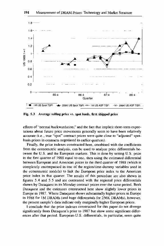
191 Measurement of DRAM Prices: Technology and Market Structure
O J , I , I I I I I , I I I , I I I I
854 86:4 87:4 88:4 Quarter
1 + 1 M US Spot TGFl t 256K US Spot TGFl -jy- 1 M US ASP TGFl * 256K US ASP TGFl 1 Fig. 5.3 Average selling price vs. spot basis, first shipped price
effects of “normal backwardation,” and the fact that implicit short-term expec- tations about future price movements generally seem to have been relatively accurate (i.e., true “spot” contract prices were quite close to “adjusted” spot- basis prices in contracts negotiated in earlier quarters).
Finally, the price indexes constructed here, combined with the coefficients from the econometric analysis, can be used to analyze price differentials be- tween the U.S. and the European markets. This is done by setting U.S. price in the first quarter of 1988 equal to one, then using the estimated differential between European and American prices in the third quarter of 1988 (which is completely encompassed in one of the regiodtime-dummy variables used in the econometric models) to link the European price index to the American price index in that quarter. The results of this procedure are also shown in figures 5.4 and 5.5 and are contrasted with the regional price differentials shown by Dataquest in its Monday contract prices over the same period. Both Dataquest and the estimates constructed here show slightly lower prices in Europe in 1987. Where Dataquest shows substantially higher prices in Europe in 1988 for 1M DRAMs (and huge differentials for 256K DRAMs), however, the present sample’s data indicate only marginally higher European prices.
I conclude that the price indexes constructed for this paper do not diverge significantly from Dataquest’s prior to 1987 but show some significant differ- ences after that period. European-U.S. differentials, in particular, seem quite

Table 5.7 Approximate Time-Series Generalized Fisher Ideal DRAM Price Indices, 1988:l = 1, ("spot-basis'' first shipment contract prices)
1M DRAM 256K DRAM 64 K DRAM
E Basis U Basis S Basis E Basis U Basis S Basis E Basis U Basis S Basis
VWCP TFGI VWCP TGFI VWCP TGFI VWCP TGFl VWCP TGFI VWCP TGFI VWCP TGFI VWCP TGFI VWCP TGFI
19852 19853 1985:4 1986: 1 19862 1986:3 1986:4 1987: 1 1987:2 1987:3 1987:4 1988: 1 1988:2 1988:3 1988:4 1989: 1
NA NA NA NA NA NA NA
0.91 0.78 0.77 0.71 1 .OO 1.06 1.17 1.13 1.06
NA NA NA NA NA NA NA
0.91" 0.80" 0.78'' 0.72'' 1 .OO 1.01c 1.17 1.14* 1.04
NA NA NA NA NA
0.68 NA NA NA
0.86 0.70 1 .OO 1.02 1.04 1.01 1.01
NA NA NA NA NA
0.71a NA NA NA
0.87b 0.71b 1 .OO 1.02c 1.04 1.02d 1 .OO
NA NA NA NA NA
0.75 NA
0.86 0.74 0.73 0.67 1 .OO 1.02 1.11 1.10 1.03
NA 0.89 O.9le NA 1.05 1.05 NA NA NA NA 0.72 0.63 NA 0.86 0.78'
0.71" 0.86 0.74 NA NA NA
0.840 0.78 0.75" 0.74" 0.96 0.89" 0.73b 0.85 0.85" 0.67b NA 0.818 1.00 1.00 1.00 0.97' 1.17 1.15'' 1.10 1.24 1.35 1.1W 1.29 1.17h 1.02 1.58 1.56
0.91 1.0s" 1.06 1.22 NA NA
0.74 0.73 0.70 0.72' 0.88 0.87
NA NA 0.83 0.85" 0.86 0.90" 0.87 0.91"
NA 0.838 1.00 1.00 1.21 1.21h 1.26 1.27 1.18 1.07h 1.40 1.40
0.90 0.99' 1.05 1.13 NA NA
0.73 0.68 0.77 0.75' 0.87 0.81
NA NA 0.76 0.75" 0.89 0.89" 0.86 0.88'
NA 0.828 1.00 1.00 1.19 1.17'' 1.26 1.37 1.35 1.21" 1.61 1.61
0.50 0.49
NA NA 0.57 0.58 0.72 0.74 0.79 0.77
NA NA 0.86 0.85 0.80 0.80 0.60 0.4gk 1.23 1.32' 1.00 1.00 1.54 1.52 NA NA NA NA
1.84 1.75
0.50 0.471 0.67 0.67
NA 0.76 0.97 1.05 NA
0.89 0.81 0.60 1.23 1 .OO 1.54 NA NA
1.67
0.66' 0.631 NA
0.77 0.99 1.03 NA
0.88 0.81 0.4gk 1.32' 1 .OO 1.52 NA NA
1.59
0.50 0.49
NA NA 0.57 0.58 0.75 0.76 0.79 0.77
NA NA 0.85 0.85 0.79 0.79 0.60 0.4gk 1.12 1.20' 1.00 1.00 1.53 1.48 NA NA NA NA
1.67 1.62
0.50 0.471

Table 5.7 (continued)
Note: See the text. The Time-series Generalized Fisher Ideal price index uses the first quarter of each year as a benchmark quarter, then takes the geometric mean of quarterly Paasche and Laspeyres indexes between adjoining benchmark quarters. Four-quarter sequences of TGFI indexes are then linked at benchmark quarters; comparisons between adjoining pairs of benchmark quarters are true Fisher Ideal comparisons. Underlying Paasche and Laspeyres index numbers cannot be calculated when some needed price data are missing or unavailable; available data has been used to impute unobserved price changes and chain to adjacent quarters when possible. Unless otherwise noted, the Laspeyres (starting-quarter weights) index is chained back to the previous quarter; the Paasche (ending-quarter weights) index is chained forward to the following quarter. This procedure imputes a rate of change for missing prices equal to the weighted average of available prices, and has been applied as follows: Chained to 1988:l using 120 ns, 1M X 1; bChained using 100 ns, 1M X 1; Chained using 100 and 120 ns, 1M X I ; Thained using 100 ns, IM X 1; 'Chained to 1985:3 using 150 ns, 256K X 1; 'Chained using 150 ns, 256K X 1; Chained to 1987:3 using 100 ns, 256K X 1; "Chained using 120 and 150 ns, 256K X I ; 'Chained to 1986:l using 150 and 120 ns, 64K X 1; Chained to 1986:l using 150 ns, 64K X 1; kLaspeyres chained to 1987:2, Paasche to 1988:1, using 120 ns, 64K X 1; 'Laspeyres chained to 1987:2, Paasche to 1988:l using 150 ns, 64K X 1. In 1987, the Paasche index cannot be calculated for some quarters in which new products introduced that year were not purchased by firms in the sample. In this case, a subindex for products excluding the newly introduced item was calculated and used (as discussed in the text, this probably creates some positive bias). The following two products were excluded in these cases: m120 ns, 256K X 4 excluded; '120 ns, 64K X 4 excluded. VWCP = Volume weighted contract price, all chip types; TGFI = approximate Time-series Generalized Fisher Ideal price index; E = European customer basis; U = United States customer basis; S = sample basis.

194 Kenneth Flamm
2-
- 1 5 - II
OD co v) 3
v
0 5-
L256K DRAMs 1
I - - -
-’“ I \
0“ I , I I I I I , , , I , I I I , 85:4 8614 87:4 88:4
Quarter
f US Spot TGFl t Europe Spot TGFl + DQ Monday US Book ++ DQ Monday Eur Book +- U.S. Retail Spot
-x- Dataquest Wwide ASP
Fig. 5.4 256K DRAMs: US.-Europe price indexes and differentials
exaggerated in the Dataquest figures, and the timing of 1988 increases in 1M DRAM contract prices seems to lag the present estimates somewhat. Table 5.8 displays two variants of annual price indexes based on Dataquest’s esti- mated average selling prices for 256K DRAMs with another consulting firm’s average-selling-price estimates and a “spot-basis’’ booking price series devel- oped in this paper. As can be seen, the billing price estimates from Integrated Circuit Engineering (ICE) and my price index generally track each other better than either price index based on Dataquest estimates.43
5.6 Conclusion
Semiconductor memory is thought to have experienced one of the most rapid rates of decline in quality-adjusted price yet measured by economists, exceeding even that of computers. Examination of this question is compli- cated by the extraordinary rate of introduction of new products embodying technical change and by the complexity of the sales channels and contractual
43. Note that the (unweighted quarterly average) Dataquest price for 256K DRAMs used by Dulberger, and reproduced in this table for direct comparison with my price index, behaves very differently from Dulberger’s “MOS memory” price index as reproduced in Triplett’s comparison table in this volume.
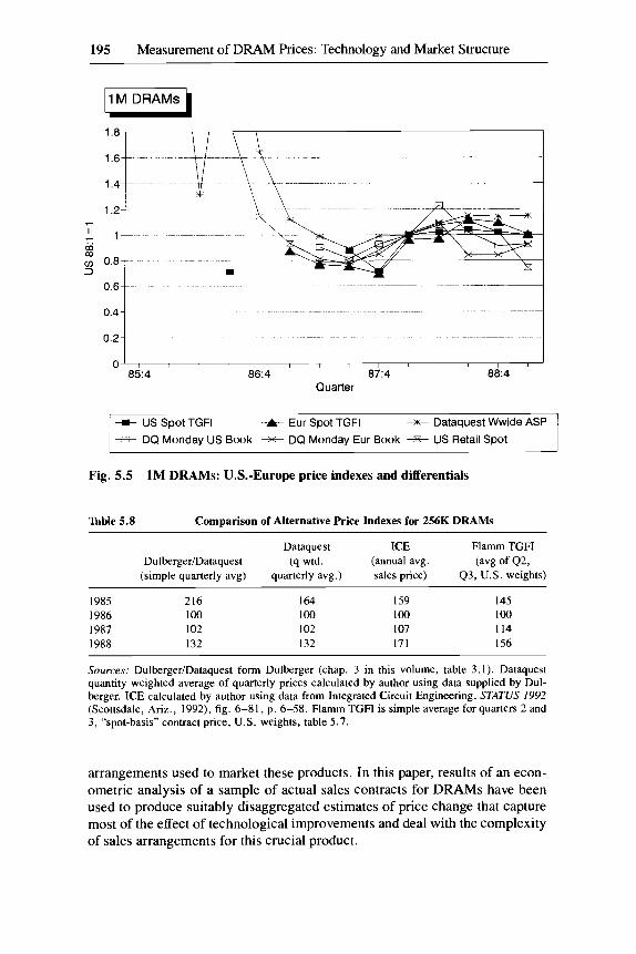
195 Measurement of DRAM Prices: Technology and Market Structure
0 ‘ I 1 I , I I I , I I 1 I
8514 86:4 87:4 88:4 Quarter
f US Spot TGFl -t Eur Spot TGFl ++ DQ Monday US Book + DQ Monday Eur Book + US Retail Spot
s Dataquest Wwide ASP
Fig. 5.5 1M DRAMs: U.S.-Europe price indexes and differentials
Table 5.8 Comparison of Alternative Price Indexes for 256K DRAMs
Dataquest ICE Flamm TGFI Dulberger/Dataquest (q wtd. (annual avg. (avg of 4 2 ,
(simple quarterly avg) quarterly avg.) sales price) 4 3 , U.S. weights)
1985 216 1986 100 1987 102 1988 132
164 100 102 132
159 100 107 171
145 100 I14 156
Sources: DulbergeriDataquest form Dulberger (chap. 3 in this volume, table 3.1). Dataquest quantity weighted average of quarterly prices calculated by author using data supplied by Dul- berger. ICE calculated by author using data from Integrated Circuit Engineering, STATUS 1992 (Scottsdale, Ariz., 1992), fig. 6-81, p. 6-58. Flamm TGFI is simple average for quarters 2 and 3, “spot-basis” contract price, U.S. weights, table 5.7.
arrangements used to market these products. In this paper, results of an econ- ometric analysis of a sample of actual sales contracts for DRAMs have been used to produce suitably disaggregated estimates of price change that capture most of the effect of technological improvements and deal with the complexity of sales arrangements for this crucial product.

196 Kenneth Flamm
The empirical results for the period 1985-89 suggested that using simple, volume-weighted average cost per chip, aggregated across chip speeds and organizations, may be a tolerable shortcut in producing an estimate of quality- adjusted cost for some given DRAM density, if long-run trends, rather than particular quarter-to-quarter changes, are the object of interest. The price se- ries constructed here differ in some important respects from the widely used Dataquest estimates, in the timing of some significant changes in price and the magnitude of regional price differentials. Given the straightforward, well- defined description of my sample and procedures, these estimates, or ones like them, are probably preferable for economic research purposes.
A relatively low-cost data collection effort-possibly including the use of advertised prices as well as contract data provided by large consumers-could be used to improve price index construction. Timely and frequent updating of sampling procedures is clearly crucial in producing any accurate price index for a good like DRAMS, where frequent and massive shifts in consumption patterns, toward innovative new products, regularly occur. The proliferation of government policies affecting the semiconductor market means that accu- rate information that would permit one to track the effects of economic policy should now be a high priority on the statistical agenda.
References
Chari, V. V., and Ravi Jagannathan. 1990. The simple analytics of commodity futures markets: Do they stabilize prices? Do they raise welfare? Federal Reserve Bank of Minneapolis Quarterly Review (3): 12-24.
Diewert, W. Erwin. 1978. Superlative index numbers and consistency in aggression. Econometrica 46: 883-900.
. 1987. Index numbers. In The new Palgrave: A dictionary of economics, ed. John Eatwell, Murray Milgate, and Peter Newman. London: Macmillan.
Flaherty, M. Therese, and Kathryn S. H. Huang. 1988. The myth of the shortening product life cycle. Harvard Business School. Typescript.
Flamm, Kenneth. 1989. Policy and politics in the international semiconductor indus- try. In Information services seminar 1989. Mountain View, Calif.: Semiconductor Equipment and Materials Institute.
. 1990. Semiconductors. In Europe 1992: An American perspective, ed. Gary C . Hufbauer. Washington, D.C.: Brookings.
. 1993. Mismanaged trade? Strategic policy in semiconductors. Washington, D.C.: Brookings.
Houthakker, H. S. 1987. Futures trading. In The new Palgrave: A dictionary of eco- nomics, ed. John Eatwell, Murray Milgate, and Peter Newman. London: Macmil- Ian.
Newbery, D. M. G. 1987. Futures markets, hedging, and speculation. In The new Palgrave: A dictionary of economics, ed. John Eatwell, Murray Milgate, and Peter Newman. London: Macmillan.

197 Comment (chaps. 3, 4, and 5 )
Newbery, D. M. G . , and J. E. Stiglitz. 1981. The theory of commodity price stabili-
Stein, Jerome L. 1987. The economics of futures markets. London: Blackwell. Triplett, Jack E. 1989a. Price and technological change in a capital good: A survey of
research on computers. In Technology and capital formation, ed. Dale W. Jorgenson and Ralph Landau. Cambridge, Mass.: MIT Press.
. 1989b. Superlative and quasi-superlative indexes of price and output for in- vestment goods: Office, computing, and accounting machinery. Discussion Paper no. 40. Washington, D.C.: Bureau of Economic Analysis.
U.S. International Trade Commission (USITC). 1985. 64K dynamic random access memory components from Japan. Publication no. 1735. Washington, D.C.
. 1986. 64K dynamic random access memory components from Japan. Publi- cation no. 1862. Washington, D.C.
Williams, Jeffrey. 1986. The economic function of futures markets. Cambridge: Cam- bridge University Press.
zation. Oxford: Clarendon.
Comment Jack E. Triplett
This session contains three studies of a single product. Estimating the trend of semiconductor prices is of interest in itself, owing to the role of semiconduc- tors as carriers of much of the high-tech electronic revolution of the last thirty years.
The session also provides evidence on a major puzzle of government price statistics-the contradictory and anomalous behavior of the Bureau of Eco- nomic Analysis (BEA) computer price index and producer price index (PPI) semiconductor price indexes. The PPI for semiconductors declines at a mod- est rate that is clearly inconsistent with the dramatic decline of computer prices (see the left-hand columns of table C.2). Semiconductors are major inputs to the computer industry. They are also important technological con- tributors to the advances in computer capability. To paraphrase Denison (1989), how can computer prices fall so fast if the prices of semiconductor inputs to the computer industry do not? Are the computer price indexes in error, as Denison suggests, or are there problems in the semiconductor price indexes?
Alternatively, we might ask this question another way. If the PPI semicon- ductor price measures are right, an enormous increase in productivity in the computer industry is implied by the computer price indexes that are prepared by the BEA; is this plausible? The first section that follows discusses the price index issues; the second turns to the productivity questions.
Jack E. Triplett is chief economist of the Bureau of Economic Analysis, U.S. Department of
Copyright is not claimed for this comment. Commerce.

198 Jack E. Piplett
Table C.2 Comparison of Price Indexes for U.S. Computers and Semiconductors (1982 = 100 unless specified)
Flamm
(1988:l = 100)
PriceIndex 3674 3674P MOS MOS Memory and Jang 256P 1 M
Year (1) (2) (3) (4) ( 5 ) (6) (7) (8)
1974 789 110 287 8,251 5,739
PPI Semiconductors (DRAM)
NIPA Computer Dulberger, Norsworthy
1975 704 113 NA 2,601 3,265 1976 665 107 212 1,592 1,852 1977 474 101 210 998 1,087 1978 242 95 187 584 64 1 1979 205 94 169 496 395 1980 147 101 NA 353 259 1981 119 101 NA NA I66 163 1982 100 99 96 101 100 I00 1983 94 101 96 NA 71 68 1984 77 107 101 101 55 49 1985 51 107 95 73 21 32 108 NA 1986 47 108 94 62 14 23 72 71b 1987 40 108 92 63 12 NA 90 87b 1988 38 108 93 75 13 NA 121 102 1989 36 108 92 . . . NA NA 140' 100'
Sources: Column 1 : Bureau of Economic Analysis, unpublished price index for computer processors (mainframes). Column 2: Producer price index, Bureau of Labor Statistics, LABSTAT series PCU 3674# (includes secondary products and miscellaneous receipts). Column 3: Producer price index, Bu- reau of Labor Statistics, LABSTAT series PCU 3674#P (primary products only). Column 4: Producer price index, MOS memory (taken from Dulberger, chap. 3 in this volume, table 3.7). Column 5: Dul- berger (chap. 3 in this volume, table 3.7; Fisher Ideal chain index). Column 6: Norsworthy and Jang (chap. 4 in this volume, table 4A.7 [price index for semiconductors used in SIC 3575, computer manu- facturing], rebased to 1982 = 100). Column 7: Flamm (chap. 5 in this volume, table 5.7), Time-series Generalized Fisher Ideal indexes for U.S. DRAM customers. Note: NA = not available. 'Second quarter of the year, unless otherwise specified. bThird quarter. cFirst quarter.
Price Index Issues
Is the Semiconductor PPI Right?
All three studies present evidence suggesting that the PPI for semiconduc- tors is not right, that correctly measured price indexes for semiconductors would fall rapidly, perhaps as fast as computer prices (see table C . 2 ) . Two of the three studies (Dulberger; Norsworthy and Jang) present price indexes for semiconductors for fairly long time series. Both studies show enormous drops in semiconductor prices; these drops contrast sharply with the modest declines that are recorded in the PPI.
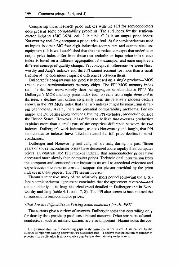
199 Comment (chaps. 3, 4, and 5)
Comparing these research price indexes with the PPI for semiconductors does present some comparability problems. The PPI index for the semicon- ductor industry (SIC 3674, col. 2 in table C.2) is an output price index; Norsworthy and Jang compute a price index (col. 6) for semiconductors used as inputs in other SIC four-digit industries (computers and communications equipment). It is well established that the theoretical concepts that underlie an output price index differ from those that underlie an input price index: each index is based on a different aggregation, for example, and each employs a different concept of quality change. Yet conceptual differences between Nors- worthy and Jang’s indexes and the PPI cannot account for more than a small fraction of the enormous empirical differences between them.
Dulberger’s comparisons are precisely focused on a single product-MOS (metal oxide semiconductor) memory chips. The PPI MOS memory index (col. 4) declines more rapidly than the aggregate semiconductor PPI.’ Yet Dulberger’s MOS memory price index (col. 5) falls from eight thousand to thirteen, a decline that differs so greatly from the relatively modest decline shown in the PPI MOS index that the two indexes might be measuring differ- ent phenomena. Again, there are potential comparability problems. For ex- ample, the Dulberger index includes, but the PPI excludes, production outside the United States. However, it is difficult to believe that overseas production explains more than a small part of the empirical difference between the two indexes. Dulberger’s work indicates, as does Norsworthy and Jang’s, that PPI semiconductor indexes have failed to record the full price decline in semi- conductors.
Dulberger and Norsworthy and Jang tell us that, during the past fifteen years or so, semiconductor prices have decreased more rapidly than computer prices. In contrast, the PPI indexes indicate that semiconductor prices have decreased more slowly than computer prices. Technological information from the computer and semiconductor industries as well as anecdotal evidence and experiences of computer users all support the picture provided by the price indexes in these papers. The PPI seems in error.
Flamm’s intensive study of the relatively short period following the U.S.- Japan semiconductor agreement concludes that the agreement reversed-and quite suddenly-the long historical trend detailed in Dulberger and in Nors- worthy and Jang (table 4.1, cols. 7, 8). The PPI also seems to have missed the turnaround in semiconductor prices.
What Are the DiBculties in Pricing Semiconductors for the PPI?
The authors give a variety of answers. Dulberger notes that controlling only for density (bits per chip) produces a biased measure. Other attributes of semi- conductors, such as miniaturization, are also important. Flamm notes the cor-
1 . I presume that the disconcerting gaps in the historical series in col. 4 are caused by the number of reporters falling below the PPI disclosure rule-I believe that the minimum number of reporters for publication is three-rather than by true discontinuity in the series.
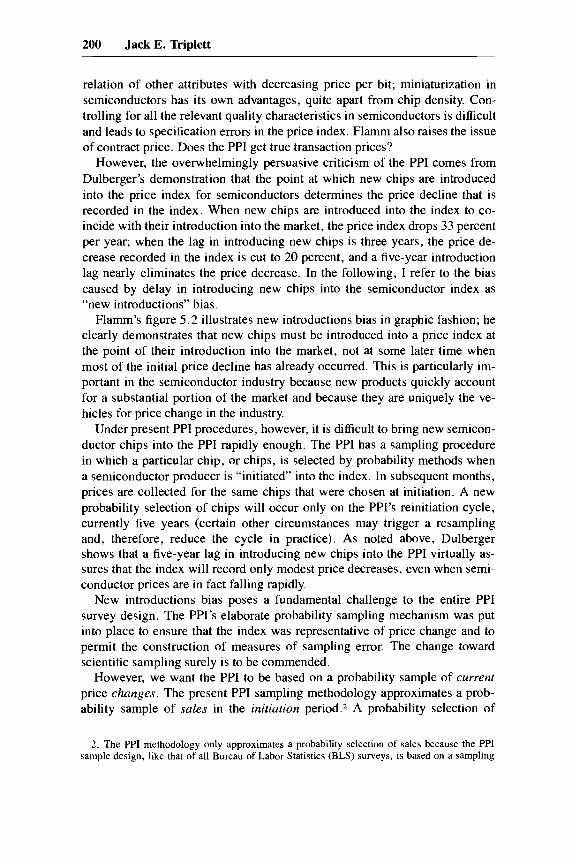
200 Jack E. Tkiplett
relation of other attributes with decreasing price per bit; miniaturization in semiconductors has its own advantages, quite apart from chip density. Con- trolling for all the relevant quality characteristics in semiconductors is difficult and leads to specification errors in the price index. Flamm also raises the issue of contract price. Does the PPI get true transaction prices?
However, the overwhelmingly persuasive criticism of the PPI comes from Dulberger’s demonstration that the point at which new chips are introduced into the price index for semiconductors determines the price decline that is recorded in the index. When new chips are introduced into the index to co- incide with their introduction into the market, the price index drops 33 percent per year; when the lag in introducing new chips is three years, the price de- crease recorded in the index is cut to 20 percent, and a five-year introduction lag nearly eliminates the price decrease. In the following, I refer to the bias caused by delay in introducing new chips into the semiconductor index as “new introductions” bias.
Flamm’s figure 5.2 illustrates new introductions bias in graphic fashion; he clearly demonstrates that new chips must be introduced into a price index at the point of their introduction into the market, not at some later time when most of the initial price decline has already occurred. This is particularly im- portant in the semiconductor industry because new products quickly account for a substantial portion of the market and because they are uniquely the ve- hicles for price change in the industry.
Under present PPI procedures, however, it is difficult to bring new semicon- ductor chips into the PPI rapidly enough. The PPI has a sampling procedure in which a particular chip, or chips, is selected by probability methods when a semiconductor producer is “initiated” into the index. In subsequent months, prices are collected for the same chips that were chosen at initiation. A new probability selection of chips will occur only on the PPI’s reinitiation cycle, currently five years (certain other circumstances may trigger a resampling and, therefore, reduce the cycle in practice). As noted above, Dulberger shows that a five-year lag in introducing new chips into the PPI virtually as- sures that the index will record only modest price decreases, even when semi- conductor prices are in fact falling rapidly.
New introductions bias poses a fundamental challenge to the entire PPI survey design. The PPI’s elaborate probability sampling mechanism was put into place to ensure that the index was representative of price change and to permit the construction of measures of sampling error. The change toward scientific sampling surely is to be commended.
However, we want the PPI to be based on a probability sample of current price changes. The present PPI sampling methodology approximates a prob- ability sample of sales in the initiation period.2 A probability selection of
2. The PPI methodology only approximates a probability selection of sales because the PPI sample design, like that of all Bureau of Labor Statistics (BLS) surveys, is based on a sampling

201 Comment (chaps. 3 , 4 , and 5)
initiation-period sales may be adequate when little change occurs in the range of products that are for sale, when yesterday’s products are pretty much the same as today’s. Or the PPI sampling procedure may work fairly well when the prices of any new products that are introduced move more or less consist- ently with those of established products. Otherwise, however, the elaborate and expensive PPI probability sampling methodology does not work and may in fact give severely biased measures of price change.
Empirically, these three papers indicate that the PPI sampling mechanism does not work in the PPI semiconductors indexes. The sampling mechanism is also problematic for pricing computers, and it is inadequate in the PPI for prescription drugs, where new introductions show price movements that differ substantially from those for established drugs (Bemdt, Griliches, and Rosett 1992). Although there is no PPI for CT scanners, the hedonic index that is presented in a paper by Trajtenberg (1990) resembles hedonic price indexes for computers far more than it resembles the PPI for medical equipment, which shows only modest declines.
All these cases are ones of technologically dynamic industries that are char- acterized by aggressive product competition. In semiconductors and comput- ers, and possibly in the other two as well, the technology gives us new prod- ucts at a cost so far below the cost implied by the old technology that the new products simply take over the market from the established ones. The prices of the established products never fall sufficiently to make them competitive with the new products. A price index that records only price movements in estab- lished products misses much of the price change that occurs in the industry.
The new introductions bias can be thought of as a “quality problem” in the price index, but it is not a quality adjustment problem. New introductions bias has nothing to do with the adequacy of the methods that are used for quality adjustment when new products are encountered in the normal production of the index, although inadequate quality adjustment methods can exacerbate the problem. It also has nothing directly to do with Laspeyres or Paasche (or even superlative index number) weighing schemes, although aspects of weighing problems may be present, may also exacerbate the problem, and may inappro- priately influence the sample design process. New introductions bias is a sam- pling problem, a case where rapid technological change creates a sample that is not representative of current price change in the industry.
The present PPI sampling methodology forces the BLS to measure techno- logically dynamic industries with a sample of old products. Reducing the in- terval between reinitiations may produce somewhat better numbers (the mag- nitude of the improvement is suggested by Dulberger’s table 3.8); however, more frequent initiations will never eliminate the problem and may not reduce
frame that contains only the establishment’s employment, not its sales. The data on the sales of the establishment are in the Census Bureau’s records, which illustrates one of the deficiencies of the irrationally organized U.S. “decentralized” statistical system.

202 Jack E. Riplett
new introductions bias to an acceptable level. What is needed is a complete rethinking of the PPI sampling methodology and possibly as well some re- thinking of the purposes of the PPI and the objectives of the PPI ~ r o g r a m . ~
Traditional PPI Methods and Hedonic Methods
Hedonic methods provide an alternative to traditional PPI methods. It is quite well established that hedonic methods can be used to develop price (and output) indexes for technologically dynamic industries, and, despite some problems, they are better than conventional methods for measuring technolog- ically dynamic products. For a review of hedonic methods from the practical vantage of a statistical agency environment, see Triplett (1990). For a review of their application to a particular high-tech industry, see Triplett (1989).
Hedonic methods can be used to construct price and output indexes for the computer industry, and for some other technological industries, because data are available annually on all the product varieties that the industry produces; hedonic indexes thus incorporate all the new products in the period in which they are introduced into the market. New introductions bias is, accordingly, absent. Hedonic methods can also be used to analyze the effects of the various ways of introducing new products into the index (see Dulberger 1989; Berndt et al. 1992).
However, hedonic price indexes are often quality-adjusted list price indexes because the most readily available cross-sectional price information usually consists of published list prices. Some transaction price errors are inevitable in hedonic indexes when discounts from list prices ~ h a n g e . ~
As noted above, the PPI sampling methodology can, in principle, get the transactions prices right, but using this methodology incurs a substantial new introductions bias. Hedonic price indexes using list prices eliminate the new introductions bias but may result in a transactions price error.
The obvious solution is to use a combination of both approaches. If the PPI sampling methodology were reoriented to collect the average discount by class of product, then these discounts could be employed to correct the he-
3. For example, in a monthly index that serves as contract escalator, it may be difficult to introduce new information that may be available only annually, or with a lag, into the measure. If the purpose of the index is analytic, gathering information on new products and the date when they were introduced leads naturally to revising the index when additional information becomes available. The present PPI is designed as if its objectives were solely of the first type; analytic objectives always, or usually, give way when conflict arises.
4. However, the error introduced by missing discounts must be small relative to new introduc- tions bias and quality-change errors in the long-term trend, at least for high-tech goods such as computers. When rebased to 1982 = 100, the computer processor index in Triplett (1989) begins at over 76,000 in 1953, falls to 856 in 1972, and winds up at 77 in 1984-i.e., the quality- adjusted (list) price index indicates that computer prices in 1984 were one-tenrh of 1 percent of their level thirty years before. No conceivable change in discounts will perceptibly affect one's views of the price change in computers over this period. Changes in list prices and transactions prices may be more important in measures of quarterly or monthly price change.

203 Comment (chaps. 3 ,4 , and 5 )
donic indexes for movements in the ratio of list prices to transactions prices. The French statistical agency is proposing to use this combined method to estimate computer prices (INSEE 1991). A similar reorientation of the tradi- tional PPI approach to price index numbers might also be fruitful in the United States.
Productivity and Technical Change Questions
What Have We Learned about the Allocation of Productivity Change?
The introduction to this comment asked whether the enormous productivity increase recorded in the computer industry was overstated. These three papers suggest that it is. The new price indexes for semiconductors that are produced by these three studies will reallocate some of the measured multifactor pro- ductivity change from the computer industry to the semiconductor i n d ~ s t r y . ~ The faster semiconductor prices decline, the greater will be the growth in the deflated (quantity) measure of semiconductor inputs used in the production of computers, and thus the slower the growth in computer industry multifactor productivity. Some of the computer industry’s reduced productivity will be transferred, in turn, to the semiconductor industry because its deflated output measure will grow more rapidly when the new price indexes for semiconduc- tors replace the PPI. These new price indexes for semiconductors will more accurately allocate the total productivity contribution of these two technolog- ically dynamic industries.
There is a corollary question that is often discussed. Why is the productiv- ity increase (price decrease) for computers so much greater than the productiv- ity increase (price decrease) for other semiconductor-using industries, partic- ularly communications equipment?
Dulberger emphasizes differences in the technology of the processes that are used by each industry. Innovations are observed in the characteristics of semiconductors (e.g., density) and also in their manufacturing processes. A second stage of technical innovation concerns the packaging of semiconduc- tors on computer cards and boards (her table 3.4 shows the relative contribu- tions of chips and packaging to the reduction in delay time). She also empha- sizes the great differences between logic chips and memory chips. The computer and communications equipment industries use different semicon- ductors, or use these chips in differing proportions, and will, therefore, bene- fit differentially.
5 . Provided that multifactor productivity studies employ ourpur in the numerator of the produc- tivity ratio (the left-hand side of the production, or cost, function), rather than computing “value- added” productivity. Output, not value-added, is the appropriate variable for production analysis. To paraphrase a remark that Evsey Domar made thirty years ago, one wants a measure of the productivity of the computer industry, not the productivity of making computers without semicon- ductors.

204 Jack E. Rkiplett
Norsworthy and Jang also conclude that the use of different semiconductors accounts for the differences in the productivity increases of these two using industries. They estimate cost functions for the two using industries and find that the quality-adjusted semiconductor prices paid by the two industries dif- fer. They give as an explanation that computers and communications equip- ment in fact use different semiconductors.
Flamm has addressed this issue elsewhere (Flamm 1989). He rejects the analogy that says that computers and communications equipment both simply move information from one place to another. In fact, the technology that each one uses is different, and the computer industry has been able to take advan- tage of technological changes in electronics more quickly than the communi- cations equipment industry. This, of course, might change in the future.
Aggregation Issues in Studying Quality Change
The semiconductors that are used in computers differ from those used in communications equipment, as Dulberger and Norsworthy and Jang con- clude, and it is plausible that these different semiconductors have different price movements. Those facts, however, transparently constitute an argument against aggregating the output of the semiconductor industry, as Norsworthy and Jang have done. Norsworthy and Jang form an aggregate semiconductor industry output measure (SIC 3674). They then employ this aggregate semi- conductor industry output measure as an input in the computer industry and in the communications equipment industry.
If computers and communications equipment use different semiconductors that have different price movements, or if they use them in differing propor- tions, one should disaggregate semiconductors into components. Then the semiconductors that are actually used in, say, communications equipment can be employed in the using-industry cost function for that industry; working with an output price index for the SIC 3679 industry-wide aggregation intro- duces misspecification. I suspect that the authors might agree and that, in a “second round,” they might pursue a more disaggregate approach.
A similar point can be made about their treatment of semiconductor char- acteristics. Norsworthy and Jang’s equation (18) suggests that the two semi- conductor characteristics (density for DRAM chips and band width for micro- processor chips) should be combined with weights that are obtained from the using industry’s cost function in order to get an aggregate measure (a) that they call “quality change.”
To understand this “quality change” measure, suppose that communications (z) and computers (c) each use only one type of semiconductor (S, and S,, respectively). Assuming that only these two types of semiconductors exist, the volume of the output of the semiconductor industry is the quantity P J , + PS, ) where Pz and Pc designate the prices for the two semiconductors.
Norsworthy and Jang seek a “quality-adjusted’’ price ( P * ) so that the output of the semiconductor industry (PJz + PJ,) can be used as an input to the
205 Comment (chaps. 3, 4, and 5 )
communications industry or the computer industry. The quality-adjusted price P* for communications semiconductors is thus defined by
(1)
In words, the quality-adjusted price P* is the “deflator” that reduces the value of the semiconductor industry’s output to make it an appropriate measure of the communication equipment industry’s input. Since in this example the communications industry uses only S,, this “deflator” must eliminate entirely the part of the semiconductor industry’s output that is not used in communi- cations equipment (i.e., P J J . A similar statement applies to computer indus- try semiconductor inputs.
In addition, as Norsworthy and Jang assume, and as Dulberger and Flamm show, if the prices of the two types of semiconductors ( P , and P,) are mismea- sured, the computation of the price P* must also correct for any measurement errors in the output of the semiconductor industry. Norsworthy and Jang’s estimating procedure, however, is as much an adjustment for the differing compositions of industry output and of using-industry input as it is as an ad- justment for what we usually term quality change.
This point indirectly brings up an important, but often neglected, point about the PPI. The revised PPI is based on the idea of output price indexes- it produces measures that are aggregated for the output of SIC four-digit in- dustries, such as the semiconductor industry. Yet many of the uses of price indexes require input aggregations-for example, semiconductors as inputs to computers, or inputs to communications equipment, and so forth. As equa- tion (1) and the previous discussion suggests, the price index for industry output may be inappropriate for input uses of price indexes. The PPIs for SIC four-digit industries may not meet the requirements of analytic data users who need alternative aggregations.
Worse, data users cannot form their own aggregations of product-code PPI indexes because the detailed indexes are not always available or because there are gaps in them (see table C.21, because aggregations other than the SIC four-digit PPIs are not produced (lower-level semiconductor aggregations might ameliorate some of the discontinuity problem shown in table C.2), and because the PPI product codes often do not match the detailed Census Bureau seven-digit product codes with which the detailed PPIs would be used. Users must, therefore, use econometric procedures (such as those of Norsworthy and Jang) that would not be necessary if the PPI program were more oriented than it is now to the needs of analytic data users.
Estimating cost functions for high-tech industries is a valuable approach for determining the relative contributions to productivity of various stages of pro- duction. I am convinced, however, that extension of the direct, tool-making approach of Dulberger and of Flamm has more potential for price index esti- mation than econometric models to correct the inadequate presentation of data from government statistical agencies.
(PJZ + PCS,)lP* = s,.

206 Jack E. Riplett
Conclusion
These are three valuable papers. Dulberger, Flamm, and Norsworthy and Jang have presented results that add to an emerging body of research on tech- nological change and on price change in high-tech industries. Most of this research shows very large price reductions for technologically dynamic indus- tries. Like some of the other studies, these three suggest that there are substan- tial deficiencies in the methodology that has traditionally been used in the PPI, certainly when it is employed on technologically dynamic products. At some point, it will be necessary to reconsider PPI methodology and to search for other methodologies that better match the economics, the technology, and the marketing practices of technologically dynamic industries.
References
Berndt, Ernst R., Zvi Griliches, and Joshua Rosett. 1992. Auditing the producer price index: Micro evidence from prescription pharmaceutical preparations. NBER Work- ing Paper no. 4009. Cambridge, Mass.: National Bureau of Economic Research, March.
Denison, Edward F. 1989. Estimates of productivity change by industry: An evaluation and an alternative. Washington, D.C.: Brookings.
Dulberger, Ellen R. 1989. The application of an hedonic model to a quality-adjusted price index for computer processors. In Technology and capital formation, ed. Dale W. Jorgenson and Ralph Landau. Cambridge, Mass.: MIT Press.
Flamm, Kenneth. 1989. Technological advance and costs: Computers versus commu- nications. In Changing the rules: Technological change, international competition, and regulation in communications, ed. Robert W. Crandall and Kenneth Flamm. Washington, D.C.: Brookings.
Institut National de la Statistique et des Etudes Economiques (INSEE). 1991. Hedonic price indexes for microcomputers in France. Paris: Division Prix de Vente Industri- als, May.
Trajtenberg, Manuel. 1990. Product innovations, price indexes and the (mis)- measurement of economic performance. NBER Working Paper no. 3261. Cam- bridge, Mass.: National Bureau of Economic Research, February.
Triplett, Jack E. 1989. Price and technological change in a capital good: A survey of research on computers. In Technology and capital formation, ed. Dale W. Jorgenson and Ralph Landau. Cambridge, Mass.: MIT Press.
. 1990. Hedonic methods in statistical agency environments: An intellectual biopsy. In Fifty years of economic measurement: The jubilee of the Conference on Research in Income and Wealth, ed. Ernst R. Berndt and Jack E. Triplett. Studies in Income and Wealth, vol. 54. Chicago: University of Chicago Press (for the National Bureau of Economic Research).