MEASUREMENT OF ATMOSPHERIC COMPOSITION · Web viewThe GAW Programme Implementation Plan builds...
52
SECTION: Table_of_Contents_Chapter Chapter title in running head: CHAPTER 16. MEASUREMENT OF ATMOSPHERIC … Chapter_ID: 8_I_16_en Part title in running head: PART I. MEASUREMENT OF METEOROLOGICAL VARI… SECTION: Chapter_book Chapter title in running head: CHAPTER 16. MEASUREMENT OF ATMOSPHERIC … Chapter_ID: 8_I_16_en Part title in running head: PART I. MEASUREMENT OF METEOROLOGICAL VARI… CHAPTER 16. MEASUREMENT OF ATMOSPHERIC COMPOSITION 16.1 GENERAL The main purpose of this chapter is to introduce readers (particularly those who are new to these measurements) to methods and specific techniques used for measuring various components of atmospheric composition and a number of related physical parameters. This is often accompanied by measurements of basic meteorological variables, as introduced in the preceding chapters. Within WMO, the Global Atmosphere Watch (GAW) Programme was established to in response to the growing concerns related to human impacts on atmospheric composition and the connection of atmospheric composition to weather and climate. GAW’s mission is focused on the systematic global observations of the chemical composition and related physical characteristics of the atmosphere, integrated analysis of these observations and development of predictive capacity to forecast future atmospheric composition changes (WMO, 2017 a ) . coordinate atmospheric composition and related physical parameter measurements taken by WMO Member countries. For further practical details on measurement activities, see the GAW reports and other references listed at the end of the chapter. The observations and analyses of the atmospheric chemical composition are needed to advance the scientific understanding of the effects of the increasing influence of human activity on the global atmosphere as illustrated by pressing societal problems such as: changes in the weather and climate related to human influence on atmospheric composition, particularly, on greenhouse gases; ozone and aerosols; impacts of air pollution on human and ecosystem health and issues involving long- range transport and deposition of air pollution; changes in UV radiation as consequences of changes in atmospheric ozone amounts and climate, and the subsequent impact of these changes on human health and ecosystems. The need to understand and identify scientifically sound measures to control the increasing influence of human activity on the global atmosphere forms the rationale of the GAW Programme (WMO, 2007 b ). The grand challenges addressed by GAW include: (a) Stratospheric ozone depletion and the increase of ultraviolet (UV) radiation at the Earth’s surface; (b) Changes in the weather and climate related to human influence on atmospheric composition, particularly greenhouse gases, and the impact on ozone and aerosols, due also to natural processes; (c) Risk reduction of air pollution on human health and issues involving long-range transport and deposition of air pollution.
Transcript of MEASUREMENT OF ATMOSPHERIC COMPOSITION · Web viewThe GAW Programme Implementation Plan builds...

SECTION: Table_of_Contents_Chapter
Chapter title in running head: CHAPTER 16. MEASUREMENT OF ATMOSPHERIC …
Chapter_ID: 8_I_16_en
Part title in running head: PART I. MEASUREMENT OF METEOROLOGICAL VARI…
SECTION: Chapter_book
Chapter title in running head: CHAPTER 16. MEASUREMENT OF ATMOSPHERIC …
Chapter_ID: 8_I_16_en
Part title in running head: PART I. MEASUREMENT OF METEOROLOGICAL VARI…
CHAPTER 16. MEASUREMENT OF ATMOSPHERIC COMPOSITION
16.1 GENERAL
The main purpose of this chapter is to introduce readers (particularly those who are new to these measurements) to methods and specific techniques used for measuring various components of atmospheric composition and a number of related physical parameters. This is often accompanied by measurements of basic meteorological variables, as introduced in the preceding chapters. Within WMO, the Global Atmosphere Watch (GAW) Programme was established to in response to the growing concerns related to human impacts on atmospheric composition and the connection of atmospheric composition to weather and climate. GAW’s mission is focused on the systematic global observations of the chemical composition and related physical characteristics of the atmo-sphere, integrated analysis of these observations and development of predictive capacity to fore-cast future atmospheric composition changes (WMO, 2017a). coordinate atmospheric composition and related physical parameter measurements taken by WMO Member countries. For further prac-tical details on measurement activities, see the GAW reports and other references listed at the end of the chapter.
The observations and analyses of the atmospheric chemical composition are needed to advance the scientific understanding of the effects of the increasing influence of human activity on the global atmosphere as illustrated by pressing societal problems such as: changes in the weather and climate related to human influence on atmospheric composition, particularly, on greenhouse gases; ozone and aerosols; impacts of air pollution on human and ecosystem health and issues involving long-range transport and deposition of air pollution; changes in UV radiation as con-sequences of changes in atmospheric ozone amounts and climate, and the subsequent impact of these changes on human health and ecosystems. The need to understand and identify scientific-ally sound measures to control the increasing influence of human activity on the global atmo-sphere forms the rationale of the GAW Programme (WMO, 2007b). The grand challenges ad-dressed by GAW include:
(a) Stratospheric ozone depletion and the increase of ultraviolet (UV) radiation at the Earth’s surface;
(b) Changes in the weather and climate related to human influence on atmospheric composition, particularly greenhouse gases, and the impact on ozone and aerosols, due also to natural processes;
(c) Risk reduction of air pollution on human health and issues involving long-range transport and deposition of air pollution.
In addition, measurements of atmospheric composition are essential for understanding the radiation budget of the atmosphere and improving numerical weather prediction.
The GAW observations monitoring system focuses on six classes of variables:

2 PART I. MEASUREMENT OF METEOROLOGICAL VARIABLES
(a) Ozone: column (total) ozone and ozone vertical profiles with a focus on the stratosphere and upper troposphere;
(b) Greenhouse gases: carbon dioxide CO2 (including Δ14C, δ13C and δ18O in CO2, and oxygen/nitrogen (O2/N2) ratios), methane CH4 (including δ13C and δD in CH4), nitrous oxide (N2O) and halogenated compounds (SF6);
(c) Reactive gases: surface and tropospheric ozone (O3), carbon monoxide (CO), volatile organic compounds (VOCs), nitrogen oxides (NOx), sulphur dioxide (SO2) and molecular hydrogen (H2), ammonia (NH3)1;
(d) Atmospheric wet total2 deposition (focused largely on major ions in the wet deposition group);
(e) Ultraviolet radiation;
(f) Aerosols (including physical properties, size distribution and chemical composition).
A number of ancillary parameters are recommended for measurement at GAW stations:
(a) Solar radiation;
(b) Major meteorological parameters;
(c) Natural radioactivity including krypton-85, radon and some other radionuclides.
Atmospheric Water Vapour was tentatively included in GAW in 2015 by the decision of the Environmental Pollution and Atmospheric Chemistry Scientific Steering Committee (WMO, 2015) but the infrastructure has not been defined yet.
Due to the low mixing ratios of atmospheric trace constituents, the instruments and methods used for the quantitative and qualitative determination of atmospheric constituents are complex and sometimes difficult to operate. Small errors, for example in spectral signatures, or cross-sensitivit-ies to other compounds can easily confound the accuracy of atmospheric composition measure-ments. Therefore, besides correct operation, regular calibration of the equipment, participation in intercomparison exercises, station audits and personnel training are essential for accurate and reliable measurements. Obtaining reliable and high-quality results for most of the measurements described here is not feasible without the close involvement of specialist staff at a professional level. The main principles of the quality assurance of atmospheric composition observations within GAW are described in section 16.1.4.
The GAW Programme Implementation Plan builds around the concept of “science for services” and addresses multiple applications that utilize atmospheric chemical composition observations. The need to support air quality assessments brought new measurement techniques into the com-munity, namely low-cost environmental sensors. Low-cost air pollution sensors are a promising technology for research in atmospheric composition, monitoring local air quality and tracking hu-man exposure to air pollution (when used as a personal tracking device). The ongoing broader as-sessment reviews different sensor technologies and application-specific requirements for data quality and calibration. As this is a fast changing field continuous re-evaluation including new de-velopments and changes in performance may be required. Commission for Atmospheric Sciences plans to produce a comprehensive statement on the use of low-cost sensor technology by EC-70. These recommendations cover areas from sensor use for purely indicative measurements of air quality to their utilization as measurement instrument for improved understanding of atmospheric
1 Ammonia was identifies as one of the key substances required to address nitrogen cycle but the recommendations con-cerning measurement guidelines were not made yet.
2 Measurement techniques for the dry deposition has not been recommended yet.

CHAPTER 16. MEASUREMENT OF ATMOSPHERIC COMPOSITION 3
chemical transformations , temporal and spatial variability or long-term trends of different gases and aerosols.
16.1.1 Definitions/descriptions
Depending on the measurement principle and instrument platform, three types of measurements are routinely performed and reported, namely:
(a) Near-surface atmospheric content (from monitoring stations or mobile platforms such as ships, cars or trains);
(b) Total atmospheric column content (from surface- or space-based remote-sensing);
(c) Vertical concentration profiles (from aircraft, balloons, rockets, surface-based remote-sensing or satellite instruments).
Near-surface atmospheric content refers to the results of (continuous or discrete) measure-ments of a particular component’s quantity in an atmospheric layer of a few tens of metres above the surface at a particular location on the Earth’s surface. Results of sur-face measurements are commonly given in units of partial pressure, concentration, mixing ratio or mole fraction. The use of units that are not part of the International System of Units (SI) is strongly discouraged.
Total atmospheric column refers to the total amount of a particular substance contained in a vertical column extending from the Earth’s surface to the upper edge of the atmo-sphere. Commonly used units of total ozone are (i) column thickness of a layer of pure ozone at standard temperature and pressure conditions of 273.15 K and 101.325 kPa, respectively, and (ii) vertical column density (total number of molecules per unit area in an atmospheric column). For the other atmospheric constituents, vertical column density or column-averaged abundances are used. It is also common to report the par-tial column content of a substance, for example the tropospheric column content of NOx. Here, the vertical column that is integrated extends from the Earth’s surface to the tropopause.
The vertical concentration profile expresses the variation of the content of a trace com-pound in the atmosphere (given in the same units as near-surface content, namely par-tial pressure, concentration, number density, mixing ratio or mole fraction) as a func-tion of height or ambient pressure.
Depending on the measurement principle and instrument platform, two types of measurements are routinely performed and reported, namely:
1) point measurements and;
2) integrated measurements.
Point measurements refers to the results of (continuous or discrete) measurements of a particular component’s quantity in a specific place in space (either in an atmospheric layer of a few tens of metres above the surface at a particular location on the Earth’s surface or anywhere in the tropo-sphere, the stratosphere or any other atmospheric layer). The consequence of the vertical point measurements constitute vertical profile measurement (e.g. measurements from the aircraft or balloons/sondes, rockets, etc.). The point measurements can be performed along the specific hori-zontal routes as well e.g. using mobile (ship, train, car etc.) platforms. Results of point measure-ments are commonly given in units of partial pressure, concentration, mixing ratio or mole frac-tion. The use of units that are not part of the International System of Units (SI) is strongly discour-aged.
Oksana Tarasova, 22/01/18,
See alternative definitions

4 PART I. MEASUREMENT OF METEOROLOGICAL VARIABLES
Integrated measurements refers to the integrated or averages amount of a particular substance contained in a atmosphere along the observational path. This could be a vertical total column ex-tending from the Earth’s surface to the upper edge of the atmosphere. Commonly used units of total ozone are (i) column thickness of a layer of pure ozone at standard temperature and pressure conditions of 273.15 K and 101.325 kPa, respectively, and (ii) vertical column density (total num-ber of molecules per unit area in an atmospheric column). For the other atmospheric constituents, vertical column density or column-averaged abundances are used. It is also common to report the partial column content of a substance, for example the tropospheric column content of NOx. Here, the vertical column that is integrated extends from the Earth’s surface to the tropopause. DOAS instruments allow for the measurements of average amount of substance along horizontal path-ways as well.
Observations of atmospheric composition include gaseous composition, aerosol and precipitation total atmospheric depositionchemistry. The characteristics of the precipitation chemical composi-tion (wet deposition) are given in section 16.5. The variables describing aerosols (physical and chemical properties) are listed in section 16.6.
16.1.2 Units and scales
The following units are used to express the results of atmospheric trace compound observations:
Number of molecules per unit area: represents the column abundance of atmospheric trace com-pounds. Still widely used is the Dobson unit (DU), which corresponds to the number of molecules of ozone required to create a layer of pure ozone 10–5 m thick at standard temperature and pressure (STP). Expressed another way, 1 DU represents a column of air containing about 2.686 8 ∙ 1016 ozone molecules for every square centimetre of area at the base of the column.
Mass concentration mkg/m3
Milliatmosphere centimetre (m-atm-cm): A measure of total ozone equal to a thickness of 10–3 cm of pure ozone at STP (1 m-atm-cm is equivalent to 1 DU).
Mole fractions of substances in dry air (dry air includes all gaseous species except water vapour (H2O):
µmol/mol = 10–6 mole of trace substance per mole of dry airnmol/mol = 10–9 mole of trace substance per mole of dry airpmol/mol = 10–12 mole of trace substance per mole of dry air
Dry mole fraction requires either drying of air samples prior to measurement or correcting the measurement for water vapour abundance. When drying is impossible or the correction would add substantial uncertainty to the measurement, wet mole fractions can be reported instead. This must be clearly indicated in the metadata of the observational record.
The appropriate unit for expressing amount of substance is dry-air mole fraction, reported as ppm (parts per million, i.e. µmol/mol), ppb (parts per billion, i.e. nmol/mol) or ppt (parts per trillion, i.e. pmol/mol). A “v” has often been appended to these units to indicate mixing ratio by volume. When reporting mole fractions as volume mixing ratios, one assumes the atmosphere to be an ideal gas. Deviations from the ideal under GAW conditions can be large (such as for CO2), so the use of mole fraction is strongly preferred because it does not require an implicit assumption of ideality of the gases and, more importantly, because it is also applicable to condensed-phase species. In general, the use of SI units is highly recommended.
Isotope or molecular ratios:
CHAPTER 16. MEASUREMENT OF ATMOSPHERIC COMPOSITION 5
Atmospheric molecules can be present in different isotopic configurations.3 Isotope ratio data are expressed as deviations from an agreed upon reference standard using the delta notation:
(16.1)
δ-Values are expressed in multiples of 1 000 (‰ or per mil).
The international reference scale (i.e. the primary scale) for δ13C is Vienna Pee Dee Belemnite (VPDB). NBS 19 and LSVEC (Coplen et al., 2006) are the primary international reference materials defining the VPDB scale. For δ18O, multiple scales are in use (VPDB, Vienna Standard Mean Ocean Water (VSMOW), air-O2).
The delta notation is also used to express relative abundance variations of O2/N2 (and argon/nitro-gen (Ar/N2)) ratios in air:
(16.2)
The respective international air standard is not yet established. The Scripps Institution of Oceano-graphy (SIO) local O2/N2 scale, based on a set of cylinders filled at the Scripps Pier, is the most widely used scale.
δ(O2/N2) values are expressed in multiples of 106 or per meg.
Precipitation chemistry (wet deposition) observations include measurements of several parameters which are described in more detail in section 16.5. The following units are used:
(a) pH measurements are expressed in units of acidity defined as: pH = –log10 [H+], where [H+] is expressed in mole L–1 ;
(b) Conductivity is expressed in µS cm–1 (microsiemens per centimetre), a unit commonly used for measuring electric conductivity;
(c) Acidity/alkalinity is expressed in µmole L–1 (micromole per litre);
(d) Major ions content is expressed in mg L–1 (milligram per litre).
Aerosol observations of volumetric quantities, i.e. the amount of substance in a volume of air, are reported for STP. These may refer to a particle number concentration (cm–3), an area concentration (m2 m–3, or m–1) or a mass concentration (µg m–3). Aerosol optical depth is a dimensionless quant-ity. Absorption coefficient is expressed in m–1 .
16.1.3 Measurement principles and techniques
The existing techniques for atmospheric chemical composition measurements can be separated into three main groups: passive sampling, active sampling and remote-sensing techniques. Essen-tially, active techniques draw the air sample through the detector or sampling device by a pump, whereas passive techniques use the diffusion of air to the sampling device. In remote-sensing techniques, the analysed air volume and the detector are at different locations. Total or partial column measurements are possible only with remote-sensing techniques.
3 CO2, for example, mostly consists of 12C16O16O, while the smaller abundance higher-mass isotopologues from mass 45 up to mass 49 (13C16O16O, 14C16O16O, or 12C18O16O, the corresponding 17O siblings and the mixed-isotope species) are also found in the atmosphere.

6 PART I. MEASUREMENT OF METEOROLOGICAL VARIABLES
In the case of active sampling, measurements can either be done continuously (or at least quasi-continuously with short integration times)4 or samples can be collected or specially prepared (in glass or stainless steel cylinders, on sorbent substrates or filters) and analysed offline in special-ized laboratories. The collection of discrete samples entails the storage of samples. During this time, flask properties may influence the composition of the sample due to chemical or surface ef-fects or permeation through sealing polymers. This demands careful tests of the sampling contain-ers.
The analytical techniques most commonly used (and recommended in the GAW Programme) for detecting and quantifying atmospheric trace constituents can be summarized as follows:
(a) Spectroscopic methods refer to the measurement of changes in radiation intensity due to absorption, emission, photoconductivity or Raman scattering of a molecule or aerosol particle as a function of wavelength. Spectral measurement devices are referred to as spectrometers, spectrophotometers, spectrographs or spectral analysers. Spectral measurements can be performed in different parts of a spectrum depending on the component to be measured, or on several individual wavelengths. As absorption lines are different for molecules with different isotopic composition, and line shapes depend on the bulk composition of the gas, care should be taken to ensure that reference gases have similar properties to the analysed atmospheric air.
(b) Gas chromatography (GC) is a physical method of separation that distributes components to separate between two phases, one stationary (stationary phase), the other (the mobile phase) moving in a definite direction. There are numerous chromatographic techniques and corresponding instruments. To be suitable for GC analysis, a compound must have sufficient volatility and thermal stability. Gas chromatography involves a sample being vapourized and injected onto the head of the chromatographic column. The sample is transported through the column by the flow of inert, gaseous mobile phase. The column itself contains a liquid stationary phase which is adsorbed onto the surface of an inert solid. A chromatography detector is a device used to visualize components of the mixture being eluted off the chromatography column. There are two general types of detectors: destructive and non-destructive. The destructive detectors, such as a flame ionization detector (FID), perform continuous transformation of the column effluent (burning, evaporation or mixing with reagents) with subsequent measurement of some physical property of the resulting material (plasma, aerosol or reaction mixture). The non-destructive detectors, such as an electron capture detector (ECD), are directly measuring some property of the column effluent (for example UV absorption) and thus allow for the further analyte recovery.
(c) Mass spectrometry (MS) is an analytical technique that produces spectra of the masses of the molecules comprising a sample of material. The spectra are used to determine the elemental composition of a sample, the masses of particles and of molecules, and to elucidate the chemical structures of molecules. Mass spectrometry works by ionizing chemical compounds to generate charged molecules or molecule fragments and measuring their mass-to-charge ratios. In a number of instruments mass spectrometry can be used as a detector method for gas chromatography.
Detection methods of gases and aerosols can be different and based on different physical phenom-ena. Details on the detection methods applicable to different gases and aerosol properties are summarized in the sections below.
The measurement techniques forof the main compounds observed under the GAW Programme are briefly described in this chapter, while comprehensive measurement guidelines can be found in the specialized GAW reports, cited in individual sections. In the cases where GAW measurement guidelines or standard operating procedures are not available, links are provided to the informa-tion necessary to carry out the respective measurements. The background for the measurements of individual components can be found in the WMO Global Atmosphere Watch (GAW) Strategic Plan: 200815–201523 (WMO, 200717ab) and its addendum (WMO, 2011b). 4 This is, for example, common practice in gas chromatography measurements.
CHAPTER 16. MEASUREMENT OF ATMOSPHERIC COMPOSITION 7
Satellite remote-sensing of the atmospheric species mentioned below is treated separately in Part III, Chapter 5.
16.1.4 Quality assurance
The objectives of the GAW quality assurance (QA) system are to ensure that data reported by sta-tions are consistent, of known and adequate quality, supported by comprehensive metadata, and regionally or globally representative with respect to spatial and temporal distribution.
The principles of the GAW QA system apply to each measured variable and include:
(a) Defined data quality objectives (including tolerable levels of uncertainty in the data, completeness, compatibility requirements, etc.);
(b) Establishment of harmonized recommendations on measurement techniques and quality control (QC) procedures to reach data quality objectives (measurement guidelines and standard operating procedures);
(c) Network-wide use of only one reference standard or scale (primary standard). In consequence, there is only one institution that is responsible for this standard;
(d) Traceability to the primary standard of all measurements made by GAW stations;
(e) Use of detailed logbooks for each parameter containing comprehensive meta information related to the measurements, maintenance, and quality control actions;
(f) Regular independent assessments (including audits and comparison campaigns);
(g) Timely submission of data and associated metadata to the responsible World Data Centre as a means of permitting independent review of data by a wider community.
8 PART I. MEASUREMENT OF METEOROLOGICAL VARIABLES
The following Global Climate Observing System (GCOS) monitoring principles apply also to the GAW observations:
(a) The impact of new systems or changes to existing systems should be assessed prior to implementation;
(b) A suitable period of overlap for new and old observing systems should be required;
(c) Uninterrupted station operations and observing systems should be maintained.
The GAW QA system further recommends the adoption and use of internationally accepted meth-ods and vocabulary to describe uncertainty in measurements.
Five types of central facilities (see the annex) dedicated to the six groups of measurement vari-ables (see section 16.1) are operated by WMO Members and form the basis of the quality assur-ance and data archiving system. These include:
(a) Central Calibration Laboratories (CCLs), which host primary standards and scales;
(b) World/Regional Calibration Centres (WCCs/RCCs), which coordinate intercomparison campaigns, help with instrument calibration and perform station/lab audits;
(c) Quality Assurance/Science Activity Centres (QA/SACs), which provide technical and scientific support and coordinate cooperation between the central facilities and GAW stations;
(d) World Data Centres (WDCs), which mainly ensure dissemination and easy access of GAW data and secure the data through appropriate data archiving.
The work of the central facilities on the quality assurance of the GAW observations is supported by respective scientific advisory groups, whose tasks include assisting in the development of meas-urement procedures and guidelines, data quality objectives and, when applicable, standard operat-ing procedures, reviewing new measurement techniques and making recommendations about their applicability for the GAW observations.
16.2 (STRATOSPHERIC) OZONE MEASUREMENTS
16.2.1 Ozone total column
Measurements of total ozone are possible using remote-sensing techniques only. The most precise information on total ozone and its changes at individual sites can be obtained by measurements from the ground, for example by solar spectroscopy in the wavelength region of 300–340 nm. Within the GAW Programme, Dobson spectrophotometers (designed for manual operation) and Brewer spectrophotometers (designed for automatic operation) are used as the instruments for routine total ozone observations, thus providing two independent networks.
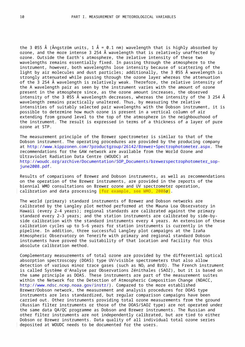
Details of the total ozone measurements with the Dobson spectrometer and their quality assur-ance are provided in WMO (2008c). Total ozone observations are made with this instrument by measuring the relative intensities of selected pairs of ultraviolet wavelengths, called the A, B*, C, C', and D wavelength pairs, emanating from the sun, moon or zenith sky. The A wavelength pair, for example, consists of the 3 055 Å (Ångström units, 1 Å = 0.1 nm) wavelength that is highly ab-sorbed by ozone, and the more intense 3 254 Å wavelength that is relatively unaffected by ozone. Outside the Earth's atmosphere, the relative intensity of these two wavelengths remains essen-tially fixed. In passing through the atmosphere to the instrument, however, both wavelengths lose intensity because of scattering of the light by air molecules and dust particles; additionally, the 3 055 Å wavelength is strongly attenuated while passing through the ozone layer whereas the at-tenuation of the 3 254 Å wavelength is relatively weak. Therefore, the relative intensity of the A wavelength pair as seen by the instrument varies with the amount of ozone present in the atmo-

CHAPTER 16. MEASUREMENT OF ATMOSPHERIC COMPOSITION 9
sphere since, as the ozone amount increases, the observed intensity of the 3 055 Å wavelength decreases, whereas the intensity of the 3 254 Å wavelength remains practically unaltered. Thus, by measuring the relative intensities of suitably selected pair wavelengths with the Dobson instru-ment, it is possible to determine how much ozone is present in a vertical column of air extending from ground level to the top of the atmosphere in the neighbourhood of the instrument. The result is expressed in terms of a thickness of a layer of pure ozone at STP.
The measurement principle of the Brewer spectrometer is similar to that of the Dobson instrument. The operating procedures are provided by the producing company at http://www.kippzonen.com/?productgroup/26142/Brewer+Spectrophotometer.aspx. The recommendations for the GAW net-work are available from the World Ozone and Ultraviolet Radiation Data Centre (WOUDC) at http://woudc.org/archive/Documentation/SOP_Documents/brewerspectrophotometer_sop-june2008.pdf.
Results of comparisons of Brewer and Dobson instruments, as well as recommendations on the operation of the Brewer instruments, are provided in the reports of the biennial WMO consultations on Brewer ozone and UV spectrometer operation, calibration and data processing (for example, see WMO, 2008a).
The world (primary) standard instruments of Brewer and Dobson networks are calibrated by the Langley plot method performed at the Mauna Loa Observatory in Hawaii (every 2–4 years); re-gional standards are calibrated against the primary standard every 2–3 years; and the station in-struments are calibrated by side-by-side calibration with the standard instruments every 4 years. An extension of these calibration cycles up to 5–6 years for station instruments is currently in the pipeline. In addition, three successful Langley plot campaigns at the Izaña Atmospheric Observat-ory on Tenerife with primary and regional standard Dobson instruments have proved the suitability of that location and facility for this absolute calibration method.
Complementary measurements of total ozone are provided by the differential optical absorption spectroscopy (DOAS) type UV/visible spectrometers that also allow detection of various minor trace gases (such as NO2 and BrO). The French instrument is called Système d'Analyse par Obser-vations Zénithales (SAOZ), but it is based on the same principle as DOAS. These instruments are part of the measurement suites within the Network for the Detection of Atmospheric Composition Change (NDACC, http://www.ndsc.ncep.noaa.gov/instr/). Compared to the more established Brewer/Dobson network, the measurement and analysis procedures for DOAS type instruments are less standardized, but regular comparison campaigns have been carried out. Other instruments providing total ozone measurements from the ground (Russian filter instruments or those of the DOAS/SAOZ type) are not operated under the same data QA/QC programme as Dobson and Brewer instruments. The Russian and other filter instruments are not independently calibrated, but are tied to either Dobson or Brewer instruments. Data quality of all individual total ozone series deposited at WOUDC needs to be documented for the users.
Care should be taken with the use of the cross sections and the most recent data should be used (WMO, 2015c).
16.2.2 Ozone profile measurements
Measurements of the vertical ozone distribution are possible by both active and remote-sensing methods.
16.2.2.1 Umkehr method
Dobson and Brewer spectrometers can be used for the measurement of vertical ozone distribution utilizing the Umkehr method (WMO, 2008c). The reduction of the Umkehr measurement to an ozone profile requires a complex algorithm that includes knowledge of the radiative properties of the real atmosphere. As this knowledge changes, the algorithm will change. A standard Umkehr observation consists of a series of C-pair wavelength measurements made on a clear zenith sky during morning or afternoon. The measurements are commenced a few minutes before sunrise
Oksana Tarasova, 22/01/18,
Need to check if the updated recommendations are available
10 PART I. MEASUREMENT OF METEOROLOGICAL VARIABLES
and continued until the sun is at an elevation of not less than about 20 degrees, or commenced in the afternoon when the sun is at an elevation of not less than about 20 degrees and continued until shortly after sunset. The zenith sky must be free from clouds for a period of 30 min to 1 h near sunrise or sunset. This is especially true at low latitude stations where the sun rises or sets rapidly. At other times, it is desirable that the zenith sky be cloudless, but permissible that clouds cross it periodically when measurements are not made. Umkehr observations cannot be made at a polar station or at high latitude stations during summertime when the sun does not sink below the horizon.
To be able to compute the vertical distribution of ozone, it is necessary to know the total amount of ozone present at the time of observation. Several total ozone measurements must, therefore, be made during the morning or afternoon, particularly if the ozone amount is changing fairly rap-idly.
The resulting ozone profile derived from reduction of these measurements is quite dependent on the algorithm used. The method of Umkehr data analysis was originally developed by Götz et al. (1934). Later the method was refined by Ramanathan and Dave (1957), Mateer and Dütsch (1964), and Mateer and DeLuisi (1992). The Umkehr algorithm is described by Petropavlovskikh et al. (2005), and updated information is available from http://www.esrl.noaa.gov/gmd/ozwv/umkehr/.
16.2.2.2 Ozonesonde measurements
Ozone measurement from light balloons (ozonesondes) is an active method for measuring the ozone vertical distribution in the atmosphere. Other active methods for ozone mole fraction meas-urements (that are used on aircraft platforms) are described in the section on reactive gases (see section 16.4.1).
Ozonesondes are small, lightweight and compact balloon-borne instruments, developed for meas-uring the vertical distribution of atmospheric ozone up to an altitude of about 30–35 km. The sens-ing device is interfaced to a standard meteorological radiosonde for data transmission to the ground station and can be flown on a small rubber balloon. Three major types of ozonesondes – the Brewer-Mast sonde, the electrochemical concentration cell and the carbon iodine cell – are nowadays in use. Each sonde type has its own specific design.
The flight package typically weighs about 1 kg in total and can be flown on small weather balloons. Normally data are taken during ascent, at a rise rate of about 5 m/s, to a balloon burst altitude of 30–35 km. The inherent response time of the ozonesonde is 20–30 s such that the effective height resolution of the measured vertical ozone profile is typically 100–150 m.
The principles of ozonesonde operations and an overview of the different aspects of quality assur-ance and quality control for ozonesonde measurements in GAW are given in detail in WMO (2014).
16.2.2.3 Other measurement techniques
Ozone profile measurements can also be obtained by other instruments operated under the um-brella of NDACC. Lidar and microwave measurements are part of the NDACC suite of measure-ments and are valuable for assessing ozone trends in the upper stratosphere and for validating satellite measurements in the upper atmosphere. The disadvantage of microwave ozone measure-ments is the rather poor vertical resolution, but they have a potential to measure up to the meso-pause region. The combination of sonde, Umkehr, lidar and microwave data from the ground is important for assessing the quality of the ozone profile measurements from space.
16.2.3 Aircraft and satellite observations
Ozone in the atmosphere is also measured by instruments located on board aircraft and space satellites. The airborne observations are usually made by in situ photometers sampling the air in the troposphere and lower stratosphere during a flight. The measurements are used mostly in re-search campaigns on atmospheric chemistry, but there have also been long-term projects using
CHAPTER 16. MEASUREMENT OF ATMOSPHERIC COMPOSITION 11
commercial aircraft, such as MOZAIC (measurement of ozone, water vapour, carbon monoxide and nitrogen oxides aboard airbus in-service aircraft), CARIBIC (Civil Aircraft for the Regular Investiga-tion of the Atmosphere Based on an Instrument Container, http://www.caribic-atmospheric.com/), and recently IAGOS (In-service Aircraft for a Global Observing System).
Large-scale monitoring of atmospheric ozone is performed by remote-sensing instruments from satellites. These programmes can be divided according to lifetime: the long-term operational mon-itoring systems that generate large (global) datasets used for trend analyses and for operational mapping of ozone, and the temporary experimental missions.
Satellite observations can be grouped according to the radiation-detection technology used for the instruments and the retrieval schemes applied for the derivation of ozone column density or con-centration from the measured radiances. While nadir-viewing instruments are primarily used for column observations and coarse vertical profiling, limb sounding instruments are able to measure vertical profiles of ozone at high vertical resolution by solar, lunar or stellar occultation or by ob-serving limb scatter and emission through the atmospheric limb (Tegtmeier et al., 2013; Sofieva et al., 2013).
16.3 GREENHOUSE GASES
All greenhouse gases are reported in dry mole fractions on the most recent scales summarized in WMO (20126cb) (status as of 20135) and reviewed every two years at the WMO/IAEA Meetings on Carbon Dioxide, Other Greenhouse Gases and Related Measurement Techniques (GGMT). The primary reference for greenhouse gases is a set of cylinders of natural air with known mole frac-tions of the studied gases. The primary scale is transferred to station working standards through secondary and tertiary gas standards in cylinders.
16.3.1 Carbon dioxide (including Δ14C, δ13C and δ18O in CO2, and O2/N2 ratios)
Carbon dioxide is usually measured by active methods in the atmospheric boundary layer.
Most of historical background atmospheric CO2 measurements are made with non-dispersive in-frared (NDIR) gas analysers, but a few programmes use a gas chromatographic method. The GC method requires separation of CO2 from other gases in the air sample, reduction of this CO2 over a catalyst with H2 to CH4, and detection of the CO2-derived CH4 using a flame ionization detector. Chromatographic peak responses from samples are compared to those from standards with known CO2 mole fractions to calculate the CO2 mole fraction in the sample. Gas chromatography tech-niques are limited to a measurement frequency of one sample every few minutes. Non-dispersive infrared instruments are based on the same principle that makes CO2 a greenhouse gas: its ability to absorb infrared radiation. They measure the intensity of infrared radiation passing through a sample cell relative to radiation passing through a reference cell. It is not necessary to know the CO2 mole fraction of the reference cell gas. Sample air, pumped from inlets mounted well away from the measurement building, and standard gas flow alternately through the sample cell. A dif-ference in CO2 concentration between sample and reference gases (or standard and reference gases) contained in the two cells results in a voltage that is recorded by the data acquisition sys-tem.
Most of the new instalments are performing the measurements of CO2 with laser-based optical spectroscopic methods, like Fourier transform infrared (FTIR) absorption spectroscopy or high-fin-esse cavity absorption spectroscopy, which includes cavity ring-down spectroscopy (CRDS) and off-axis integrated cavity output spectroscopy (ICOS). Advantageous properties of these tech-niques are reduced calibration demands due to better linearity and detector response stability.
Carbon dioxide abundances are reported in dry-air mole fraction, µmol mol–1, abbreviated ppm, on the WMO CO2 Mole Fraction Scale (WMO CO2 X2007 scale, status as of 20138). Water vapour affects the measurement of CO2 in two ways: (i) H2O also absorbs infrared radiation and can inter-fere with the measurement of CO2; (ii) H2O occupies volume in the sample cell, while standards are

12 PART I. MEASUREMENT OF METEOROLOGICAL VARIABLES
dry. At warm, humid sites, 3% of the total volume of air can be H2O vapour. The impact of water vapour on the CO2 measurement must therefore be considered. Drying to a dewpoint of –50 °C is sufficient to eliminate interferences. The novel optical spectroscopic methods often allow simultan-eous determination of the H2O vapour content, making it, in principle, possible to correct for dilu-tion due to H2O and spectroscopic effects. However, current best practice (see WMO, 20126cb) still recommends sample drying while the determination of dry-air mole fractions without sample dry-ing and the subsequent correction are under review.
An alternative method of CO2 measurement that is generally applicable to many other trace gases is the collection of discrete air samples in vacuum-tight flasks. These flasks are returned to a cent-ral laboratory where CO2 is determined by a NDIR, GC or other instrument. This method is used where low-frequency sampling (for example, once a week) is adequate to define CO2 spatial and temporal gradients, and for comparison with in situ measurements as a quality-control step. This sampling strategy has the advantage that many species can be determined from the same sample.
Measurements of O2/N2 ratios and stable isotopes of CO2 (δ13C and δ18O) help to partition carbon sources and sinks between the ocean and biosphere. Isotopic measurements are often made from the same discrete samples used for CO2 mole fraction measurements. Isotopic standards are main-tained by the International Atomic Energy Agency (IAEA), but measurement sites are part of the GAW CO2 network.
A measurement method for stable isotope determination is isotope ratio mass spectro-metry (IRMS), a specialization of mass spectrometry in which mass spectrometric methods are used to measure the relative abundance of isotopes in a given sample. The measurement set-up is described by the GAW Central Calibration Laboratory for stable isotopes at the Max Planck Institute for Biogeochemistry in Jena, Germany (http://www.bgc-jena.mpg.de/service/iso_gas_lab/pmwiki/pmwiki.php/IsoLab/Co2InAir). In recent years, optical analysers that report mole fractions of indi-vidual isotopologues have become increasingly available and are now in routine use. Many of these instruments can provide isotopic ratios with a repeatability of about 0.05‰ for δ13C of atmo-spheric CO2 and are valuable for continuous measurements. Unlike with mass spectrometric tech-niques, δ values from such instruments are often calculated from the ratio of individual measured mole fractions using tabulated absorption line strengths and are not from direct measurements of a standard material. The reference isotopic abundance is normally taken from a spectral para-meter database (typically the high-resolution transmission molecular absorption database, HITRAN) that is used in the analysis, and this does not provide a common scale such as VPDB or the Jena Reference Air Set (JRAS). Some corrections applicable to mass spectrometric methods, such as those for 17O and N2O, are not required, but other corrections, such as for interference from other atmospheric components and instrument fluctuations, may be required depending on the method used to calculate the isotopic δ values from individual mole fractions. It is important to realize compatibility between the techniques before measurement results are made public.
Measurements of the changes in atmospheric O2/N2 ratio are useful for constraining sources and sinks of CO2 and testing land and ocean biogeochemical models. The relative variations in O2/N2 ratio are very small but can now be observed by at least six analytical techniques. These tech-niques can be grouped into two categories: (i) those which measure O2/N2 ratios directly (mass spectrometry and gas chromatography), and (ii) those which effectively measure the O2 mole frac-tion in dry air (interferometric, paramagnetic, fuel cell, vacuum-ultraviolet photometric). A conven-tion has emerged to convert the raw measurement signals, regardless of technique, into equival-ent changes in mole ratio of O2 to N2. For mole-fraction type measurements, this requires account-ing for dilution due to variations in CO2 and possibly other gases. If synthetic air is used as a refer-ence material, corrections may also be needed for differences in Ar/N2 ratio. There are currently about 10 laboratories measuring O2/N2 ratios. The O2/N2 reference is typically tied to natural air delivered from high-pressure gas cylinders. As there is no common source of reference material, each laboratory has employed its own reference. There is currently no CCL for O2/N2. Hence it has not been straightforward to report measurements on a common scale, but several laboratories report results on a local implementation of the Scripps scale. There are no named versions yet.
CHAPTER 16. MEASUREMENT OF ATMOSPHERIC COMPOSITION 13
The practice of basing O2/N2 measurements on natural air stored in high-pressure cylinders ap-pears acceptable for measuring changes in background air, provided the cylinders are handled according to certain best practices, including orienting cylinders horizontally to minimize thermal and gravitational fractionation. Nevertheless, improved understanding of the source of variability of measured O2/N2 ratios delivered from high-pressure cylinders is an important need of the com-munity. An independent need is the development of absolute standards for O2/N2 calibration scales to the level of 5 per meg or better.
Atmospheric 14CO2 measurements are usually reported in Δ14C notation, the per mil deviation from the absolute radiocarbon reference standard, corrected for isotopic fractionation and for radioact-ive decay since the time of collection. For atmospheric measurements of Δ14C in CO2, two main sampling techniques are used: high-volume CO2 absorption in basic solution or by molecular sieve, and whole-air flask sampling (typically 1.5–5 L flasks). Two methods of analysis are used: conven-tional radioactive counting and accelerator mass spectrometry. The current level of measurement uncertainty for Δ14C in CO2 is 2‰–5‰, with a few laboratories at slightly better than 2‰. Recom-mendations on calibration are provided in WMO (2012b6c).
Recommendations on quality assurance of CO2 measurements (including Δ14C, δ13C and δ18O in CO2, and O2/N2 ratios) are reviewed every two years at the WMO/IAEA Meeting on Carbon Dioxide, Other Greenhouse Gases and Related Measurement Techniques. The report (WMO, 2012b6c) can be used as the most recent reference regarding calibration and measurement quality control.
16.3.2 Methane
Methane is usually measured quasi-continuously or from discrete samples by active methods in the atmosphere. Recommendations for CH4 measurements are provided in WMO (2009a).
For CH4 measurements at GAW stations, GC-FID is typically used. The analytical set-up can vary greatly depending on details such as type (manufacturer) of GC, chromatographic separation scheme used, carrier gas (such as N2 or helium (He)), data acquisition, system control hardware and software, and peak integration system. Consequently, operating procedures for the individual systems will vary.
New analysers for atmospheric measurements of CH4 based on optical methods give better repeat-ability than GC methods, but their long-term reliability is still being assessed. They are also difficult to repair in the field, and they often need to be returned to the factory for repairs. Although these instruments, which also measure water vapour, often come advertised as not needing calibration or sample drying, attendees at the 13th meeting of CO2 experts (WMO, 2006) strongly recommend that the analysers be calibrated routinely and that air samples be dried to a dewpoint of ≤ –40 °C.
16.3.3 Nitrous oxide
Nitrous oxide is usually measured by active methods in the atmospheric boundary layer. Recom-mendations for N2O measurements are provided in WMO (2009a).
A gas chromatograph equipped with an electron capture detector (GC-ECD) is widely used to sep-arate and detect N2O in ambient air. This technique offers good repeatability, but it can be difficult to implement. Because the N2O lifetime is long and its fluxes small, spatial gradients are small; therefore, their quantification requires very precise measurements. The digitized ECD signal is re-corded and integrated to quantify peak heights and areas. Collecting discrete samples of air in flasks is an alternative method of monitoring N2O. Flasks should be returned to a central laboratory for analysis by GC. Typical sampling frequencies are weekly or bi-weekly.
Updated recommendations on the measurement calibration and quality control are provided in WMO (2012b6c).
Very recently, optical analysers including high-finesse cavity absorption spectrometers with near-infrared laser sources, FTIR analysers and off-axis ICOS analysers with mid-
Oksana Tarasova, 22/01/18,
Reference should be made to the most recent 18th meeting 2016c if the statement is still correct
14 PART I. MEASUREMENT OF METEOROLOGICAL VARIABLES
infrared laser sources became commercially available for N2O. These exceed the preci-sion of gas chromatography and should allow the data quality objectives to be reached. First experiments typically show excellent performance; however, no recommendations can be made since the assessment of their long-term applicability is still in progress.
16.3.4 Halocarbons and SF6
Halocarbons and SF6 are usually measured quasi-continuously or from discrete air samples by act-ive methods in the atmospheric boundary layer. Measurement guidelines for these species are not formalized yet in the GAW Programme.
SF6 is typically measured using GC-ECD techniques on the same channel as N2O. Analytical meth-ods are described in WMO 2015d).
Global measurements of halocarbons are currently performed by the National Oceanic and Atmo-spheric Administration (NOAA) and Advanced Global Atmospheric Gases Experiment (AGAGE). The measurement histories for both NOAA and AGAGE extend back to the late 1970s. Both groups measure halocarbons using GC-ECD and gas chromatography with mass spectrometry (GC-MS) techniques. Halocarbons measured include chlorofluorocarbons (CFCs), hydrochlorofluorocarbons (HCFCs), chlorinated solvents such as CCl4 and CH3CCl3, halons, hydrofluorocarbons (HFCs), methyl halides and SF6. For many halocarbons, measurement of mole fractions in the background tropo-sphere requires sample pre-concentration. The AGAGE group operates a network of in situ sys-tems, while the NOAA group operates in situ systems (for a limited number of gases) and a flask-based programme. For more information on instrumentation and sampling sites, see: http://agage.eas.gatech.edu, http://www.esrl.noaa.gov/gmd/hats/.
16.3.5 Remote-sensing of greenhouse gases
There are several techniques used for remote-sensing of greenhouse gases. The Total Carbon Column Observing Network (TCCON, https://tccon-wiki.caltech.edu/) is a network of surface-based Fourier transform spectrometers recording direct solar spectra in the near-infrared spectral region. From these spectra, column-averaged abundances of CO2, CH4, N2O, HF, CO, H2O and HDO are re-trieved. Observations in the mid-infrared (in the NDACC network, http://www.acom.ucar.edu/irwg/) allow for accurate measurements of column-averaged abundances of CH4, N2O and CO.
16.4 REACTIVE GASES
The reactive gases considered in the GAW Programme include surface and tropospheric ozone, carbon monoxide, volatile organic compounds, oxidized nitrogen compounds and sulphur dioxide. All of these compounds play a major role in the chemistry of the atmosphere and, as such, are heavily involved in interrelations between atmospheric chemistry and climate, either through con-trol of ozone and the oxidizing capacity of the atmosphere, or through the formation of aerosols. The global measurement base for most of them is entirely unsatisfactory, the only exceptions be-ing surface ozone and carbon monoxide.
Different reference standards and methods are used in the group of reactive gases. For more stable gases, the reference material can be prepared as a cylinder filled with the air/other matrix with known gas mole fraction (for example, for CO, non-methane hydrocarbons and terpenes), while for others (such as ozone or oxidized nitrogen compounds) only reference methods/instru-ments are possible.
16.4.1 Tropospheric (surface) ozone
The detailed measurement guidelines for measuring tropospheric ozone (surface ozone is a part of tropospheric ozone measured at the Earth’s surface) are provided in WMO (2013).

CHAPTER 16. MEASUREMENT OF ATMOSPHERIC COMPOSITION 15
The mole fraction most appropriate to the chemical and physical interpretation of ozone measure-ments is the mole fraction of ozone in dry air. However, ozone measurements are usually made without sample drying, because an efficient system for drying air and leaving the ozone content of the air unchanged has not been developed. It is recommended that ozone measurements be ac-companied by measurements of water vapour mole fraction of sufficient precision that the ozone measurements could be converted to mole fractions with respect to dry air without loss of preci-sion.
A number of techniques are used for measurements of ozone in the background atmosphere. These include:
Ultraviolet absorption techniquesChemiluminescence techniquesElectrochemical techniquesCavity ring-down spectroscopy (CRDS) with NO titration Differential optical absorption spectroscopy (DOAS)Multi-axis differential optical absorption spectroscopy (MAxDOAS)Tropospheric ozone lidar
A review of each of these techniques, along with information on their applicability for use at GAW stations, is provided in WMO (2013). Note that only the first four of these techniques (those con-ducted in situ) can be traceable via a chain of calibrations to the primary standard as recommen-ded by GAW.
16.4.1.1 In situ techniques
The main principle of the UV method is based on the absorption of light in the UV region by the ozone molecule. The broad UV spectrum of ozone shows its maximum around 254 nm. This wavelength represents exactly the strongest emission line of an Hg lamp and the highest spectral sensitivity of a UV detector, which is a caesium-telluride vacuum UV diode or UV-sensitive pho-tomultiplier tube (PMT). The instrument measures the relative light attenuation between an air sample which remains unchanged (i.e. containing ozone) and one in which ozone has been re-moved. The ozone mole fraction is calculated via the Lambert-Beer law. Though UV absorption is an absolute measuring method, calibration is necessary, at least to determine the scrubber effi-ciency. Details of this measurement technique are given in WMO (2013).
Because of its high accuracy and precision, low detection limit, long-term stability, sufficient time resolution and ease of operation (almost no consumables), the UV absorption technique is recom-mended for use for routine surface ozone measurements at all GAW stations.
The advantages of the chemiluminescence methods (or chemiluminescence detection – CLD) for ozone measurements are their fast response times and high sensitivity relative to the UV method. This makes the chemiluminescence suitable for ambient air measurements which require high time resolution (such as airborne measurements). Since CLD is not an absolute method, calibra-tions are necessary. Due to its relative complexity, chemiluminescence is not recommended for routine surface ozone measurements at GAW stations. However, the chemiluminescence method is appropriate for experimental studies of ozone at GAW stations with extended programmes, as backup or for QA/QC reasons, since both instruments produce different artefacts.
All electrochemical techniques use the oxidation of iodide to iodine by O3:
Depending on the approach, the formed iodine is stabilized by former reactions or reduced at the surface of a cathode where the electrical current is measured. Like UV absorption, it is an absolute measuring method in principle. However, due to some sources of error, such as overvoltage or zero current, calibration is necessary.
16 PART I. MEASUREMENT OF METEOROLOGICAL VARIABLES
The cavity ring-down spectroscopy with NO titration is an experimental method with promise for future observations and should be incorporated into experimental studies of ozone measurements at selected GAW stations where appropriate.
16.4.1.2 Remote-sensing techniques
Remote-sensing techniques (DOAS, MAxDOAS, lidar) would require a similar traceability chain as in situ measurements, which is theoretically possible via the knowledge of the ozone cross-sections at the particular wavelengths used in the instruments. This issue is currently under consideration by the Absorption Cross Sections of Ozone (ACSO) committee.
Differential optical absorption spectroscopy is a surface-based remote-sensing method suitable for observations of several trace substances. The instrument consists of a light source, a long ambient air open optical path generally between 100 m and several km, a retro-reflector and a spectro-meter with a telescope, housed with the light source. The spectrometer observes the light source via the retro-reflector. The DOAS system uses Beer’s law to determine the ozone concentration (averaged over the light path). In principle, DOAS should be a sensitive technique, but this is con-founded by the inability of the system to regularly measure a definitive zero and determine the contribution of other UV absorbing gases and aerosols to the observed signal. The DOAS may be used as an experimental technique.
Multi-axis differential optical absorption spectroscopy is a surface-based remote-sensing method for observations of several trace substances. While this method is suitable for stratospheric monit-oring, it is also possible to apply it for trace gas profile measurements in the upper and lower tro-posphere. However, since the retrieval procedures, as well as possible tropospheric interferences, are more complicated in the lower troposphere, it needs highly experienced personnel for extract-ing and calculating the mole fractions for the respective trace gases out of the various spectra. MAxDOAS measurements of ozone, nitrogen dioxide, formaldehyde, bromine monoxide (BrO) and other species are recommended especially for providing a link between surface-based and satellite measurements at selected GAW stations with extended research programmes.
Lidar (light detection and ranging) is a surface-based remote-sensing method for observations of several trace substances. For tropospheric ozone measurements, a lidar typically uses two or more wavelengths between 266 nm and 295 nm. The chosen wavelengths are shorter than the ones used for stratospheric ozone detection (typically between 308 and 353 nm). Compared to in the stratosphere, higher ozone absorption efficiency is necessary in the troposphere in order to get enough sensitivity because of the lower ozone mixing ratios in the troposphere. Too much absorp-tion means that most light is extinguished at lower elevations, making it difficult to collect meas-urement signals from higher elevations. The extreme dynamic range of the backscattering signal over the troposphere (some decades over a few kilometres of height) is a major technical problem. Lidar tropospheric ozone measurements are recommended especially for providing a link between surface-based and satellite measurements at selected GAW stations with extended research pro-grammes.
16.4.2 Carbon monoxide
The detailed measurement guidelines for carbon monoxide measurements are provided in WMO (2010). The carbon monoxide scale is evaluated every two years together with the scales of the major greenhouse gases. For the most recent scale, please consult WMO (2012b6c).
Measurements of CO are possible both in situ and by flask collection with subsequent analysis in the laboratory. In situ continuous observations provide information about CO variability on a times-cale ranging from seconds to one hour depending on the measurement technique. In contrast to flask sampling, continuous measurements allow for near-real-time data delivery.
In situ observations can be made using a broad variety of analytical techniques. Non-dispersive infrared radiometry is based on spectral absorption at 4.7 µm. It is frequently used for continuous measurements at remote locations; however, instrument drift, limited precision and long aver-
CHAPTER 16. MEASUREMENT OF ATMOSPHERIC COMPOSITION 17
aging times are factors limiting the achievable data quality. Gas chromatography, when coupled with a number of different detectors (such as flame ionization (GC-FID) or hot mercuric oxide re-duction/UV absorption (GC-HgO)) can provide high-precision and adequate detection limits. The HgO-reduction detector tends to have a non-linear response over the range of atmospheric CO, and requires careful, repeated multipoint characterization of the detector response. The GC-FID technique requires catalytic conversion of CO to CH4. For confidence in the results, the catalytic conversion efficiency must be determined on a regular basis. This type of issue complicates efforts to properly maintain instrument calibration and provide accurate measurements. Gas chromato-graphy measurements are quasi-continuous in nature and therefore may not detect fast changes of mole fractions that can be captured by high-frequency measurements.
Several new measurement techniques have recently become available. The most established tech-nique is based on resonance fluorescence of CO (induced by a high-frequency discharge) in the vacuum ultraviolet (VURF). This method provides low detection limits with excellent precision in the range of atmospheric mixing ratios. A commercially available instrument based on VURF is used in several research laboratories, field sites and on other platforms, for example in the CARIBIC project.
Spectroscopic techniques based on CRDS and cavity-enhanced quantum cascade laser (QCL) spec-troscopy have become available. The CRDS technique operates using lasers in the near-infrared and was previously mainly used for measurements of carbon dioxide, methane and ammonia. The QCL technique measures in the mid-infrared, and commercial instruments are available that can determine both CO and N2O with a single laser. Both CRDS and QCL techniques provide CO meas-urements with low detection limits and excellent reproducibility. Tests of their long-term applicabil-ity for routine measurements at the GAW stations are still ongoing. An additional alternative with similar performance that has recently been commercialized is Fourier transform infrared absorp-tion spectroscopy.
Remote-sensing of CO column from the ground is done in the TCCON network using surface-based Fourier transform spectrometers in the near-infrared spectral region.
16.4.3 Volatile organic compounds
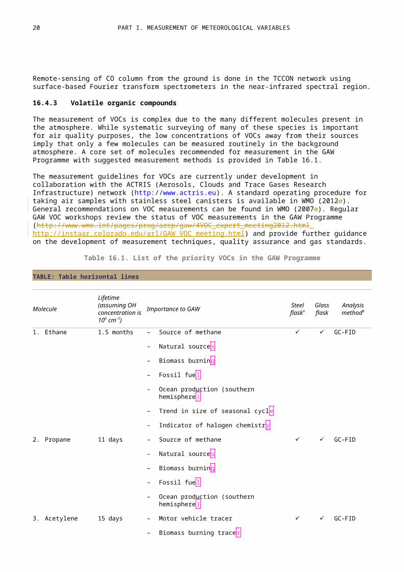
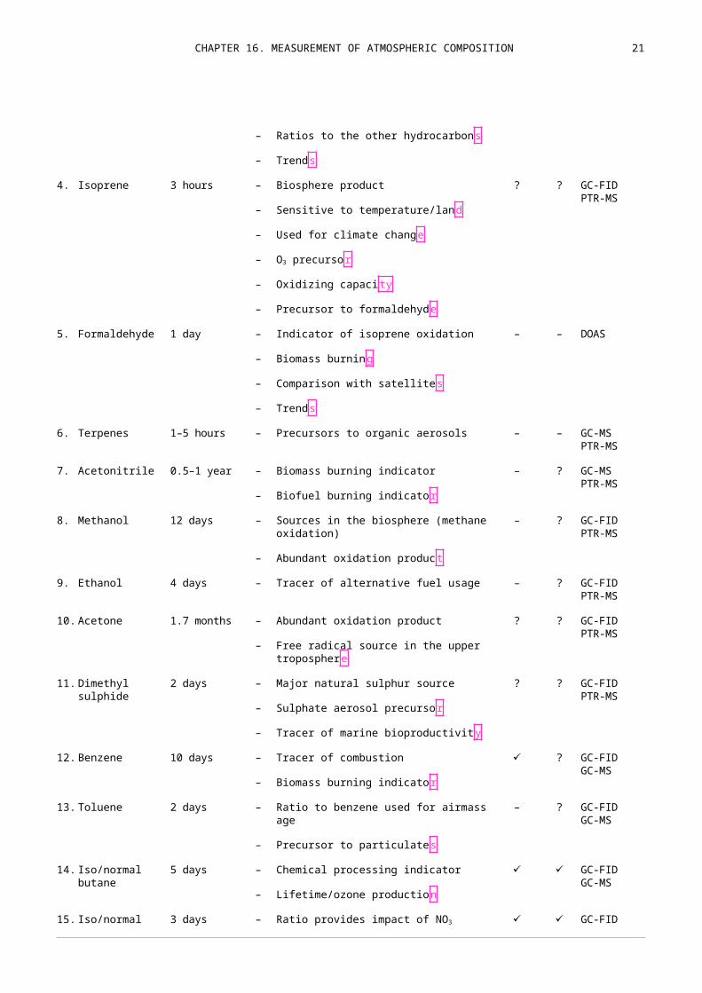
The measurement of VOCs is complex due to the many different molecules present in the atmo-sphere. While systematic surveying of many of these species is important for air quality purposes, the low concentrations of VOCs away from their sources imply that only a few molecules can be measured routinely in the background atmosphere. A core set of molecules recommended for measurement in the GAW Programme with suggested measurement methods is provided in Table 16.1.
The measurement guidelines for VOCs are currently under development in collaboration with the ACTRIS (Aerosols, Clouds and Trace Gases Research Infrastructure) network (http://www.actris.eu). A standard operating procedure for taking air samples with stainless steel canisters is available in WMO (2012a). General recommendations on VOC measurements can be found in WMO (2007a). Regular GAW VOC workshops review the status of VOC measurements in the GAW Programme (http://www.wmo.int/pages/prog/arep/gaw/4VOC_expert_meeting2012.html http://instaar.color-ado.edu/arl/GAW_VOC_meeting.html) and provide further guidance on the development of meas-urement techniques, quality assurance and gas standards.
Table 16.1. List of the priority VOCs in the GAW Programme
TABLE: Table horizontal lines
Molecule
Lifetime (as-suming OH concentration is 106 cm–3)
Importance to GAW Steel flaska
Glass flask
Analysis methodb
18 PART I. MEASUREMENT OF METEOROLOGICAL VARIABLES
1. Ethane 1.5 months – Source of methane
– Natural sources
– Biomass burning
– Fossil fuel
– Ocean production (southern hemi-sphere)
– Trend in size of seasonal cycle
– Indicator of halogen chemistry
✓ ✓ GC-FID
2. Propane 11 days – Source of methane
– Natural sources
– Biomass burning
– Fossil fuel
– Ocean production (southern hemi-sphere)
✓ ✓ GC-FID
3. Acetylene 15 days – Motor vehicle tracer
– Biomass burning tracer
– Ratios to the other hydrocarbons
– Trends
✓ ✓ GC-FID
4. Isoprene 3 hours – Biosphere product
– Sensitive to temperature/land
– Used for climate change
– O3 precursor
– Oxidizing capacity
– Precursor to formaldehyde
? ? GC-FIDPTR-MS
5. Formaldehyde 1 day – Indicator of isoprene oxidation
– Biomass burning
– Comparison with satellites
– Trends
– – DOAS
6. Terpenes 1–5 hours – Precursors to organic aerosols – – GC-MSPTR-MS
7. Acetonitrile 0.5–1 year – Biomass burning indicator
– Biofuel burning indicator
– ? GC-MSPTR-MS
8. Methanol 12 days – Sources in the biosphere (methane oxid-ation)
– Abundant oxidation product
– ? GC-FIDPTR-MS
CHAPTER 16. MEASUREMENT OF ATMOSPHERIC COMPOSITION 19
9. Ethanol 4 days – Tracer of alternative fuel usage – ? GC-FIDPTR-MS
10. Acetone 1.7 months – Abundant oxidation product
– Free radical source in the upper tropo-sphere
? ? GC-FIDPTR-MS
11. Dimethyl sulph-ide
2 days – Major natural sulphur source
– Sulphate aerosol precursor
– Tracer of marine bioproductivity
? ? GC-FIDPTR-MS
12. Benzene 10 days – Tracer of combustion
– Biomass burning indicator
✓ ? GC-FIDGC-MS
13. Toluene 2 days – Ratio to benzene used for airmass age
– Precursor to particulates
– ? GC-FIDGC-MS
14. Iso/normal bu-tane
5 days – Chemical processing indicator
– Lifetime/ozone production
✓ ✓ GC-FIDGC-MS
15. Iso/normal pentane
3 days – Ratio provides impact of NO3 chemistry ✓ ✓ GC-FIDGC-MS
Notes:
a ✓ indicates state of current practice
b GC-FID = gas chromatography flame ionization detection; GC-MS = gas chromatography mass spectrometry; DOAS = differential optical absorption spectroscopy; PTR-MS = proton transfer reaction mass spectrometry
Measurements of low molecular weight aliphatic and aromatic hydrocarbons (C2–C9) have been made successfully for many years, predominantly in short-term regional experiments. The pre-ferred analytical method for these compounds, which include the molecules 1–4 and 12–15 of Table 16.1, is GC-FID. Air samples, from flasks or in situ, are normally pre-concentrated using cryo-genic methods or solid adsorbents. An alternative technique is GC-MS. Although GC-MS is poten-tially the more sensitive method, it is typically subject to greater analytical uncertainties (changes in instrument response over time, detection of common, low-mass fragments). However, GC-MS may be valuable for the detection of certain hydrocarbons in very remote locations where ambient levels may be below the detection limit of a typical GC-FID.
The recommended analytical technique for monoterpenes is GC-MS. Although it is possible to measure some terpenes using an FID, the complexity of the chromatographic analysis (co-eluting peaks, particularly with aromatics) makes peak identification and quantification difficult. The GC-MS method gives better sensitivity.
Oxygenated hydrocarbons, including the target compounds 8–10 (Table 16.1), can also be meas-ured using GC-FID or GC-MS. Particular care should be taken with sample preparation (including water removal), and inlet systems must be designed to minimize artefacts and component losses commonly encountered with oxygenate analysis. Acetone and methanol can also be measured using proton transfer reaction mass spectrometry (PTR-MS). An advantage of PTR-MS is that it is an online method that does not require the pre-concentration of samples. However, it is less sens-itive than GC methods, and there are potential interferences from isobaric compounds, such as O2H+ and methanol. As the stability of oxygenated VOCs in grab samples (stainless steel or glass flasks) remains highly uncertain, it is suggested that these species be measured primarily by on-line methods at a selection of surface-based measurement stations. The successful storage of acetone in certain flasks has been reported, so the possibility of analysing this compound in the glass or stainless steel flask network should be investigated.
20 PART I. MEASUREMENT OF METEOROLOGICAL VARIABLES
Formaldehyde (HCHO) is not stable in flasks and has to be measured in situ. Methods of analysis include the Hantzsch fluorometric (wet chemical) method or DOAS. Both are relatively complex and would require specialist training for potential operators. It is unlikely, therefore, to be able to make measurements at more than a few ground stations. Formaldehyde is routinely detected by satellites. Satellite retrievals yield total vertical column amount, and an important objective of the GAW Programme would be to provide periodic surface-based measurements at selected sites for comparison/calibration purposes (ground truthing).
The feasibility of HCHO measurements with PTR-MS (Wisthaler et al., 2008; Warneke et al., 2011) and QCL (Herndon et al., 2007) was shown during limited measurement campaigns. Their applic-ability for long-term routine HCHO measurements has not yet been tested.
Acetonitrile is preferably measured with GC-MS, because this compound is relatively insensitive to FID detection. Measurements of acetonitrile have also been reported using various reduced gas and nitrogen-specific detectors. Many recently reported atmospheric measurements of acetonitrile have been made using PTR-MS or atmospheric pressure chemical ionization mass spectrometry (AP-CIMS). The stability of acetonitrile in grab samples is highly uncertain, so grab sampling is not acceptable in the framework of GAW and measurements may be limited to a few selected compre-hensive measurement sites.
Dimethyl sulphide (DMS) can be measured by GC-FID, gas chromatography using a flame photo-metric detector (GC-FPD), GC-MS and PTR-MS. However, as DMS concentrations can be measured routinely as part of a standard non-methane hydrocarbon (NMHC) analysis, GC-FID analysis of the whole air samples would be the simplest choice of measurement strategy. There is evidence in the literature that DMS is stable in some flasks, so its measurement as a component of a flask network is quite feasible. It is also desirable to make in situ measurements of DMS at least in the early stage of operation of the flask network to ensure method compatibility.
16.4.4 Nitrogen oxide
The sum of nitric oxide (NO) and nitrogen dioxide (NO2) has traditionally been called NOx. The sum of all nitrogen oxides with an oxidation number greater than 1 is called NOy. Their measurement in the global atmosphere is very important since NO has a large influence on both ozone and the hy-droxyl radical (OH). NO2 is now being measured globally from satellites, and these measurements suggest that substantial concentrations of this gas are present over most of the continents. A large reservoir of fixed nitrogen is present in the atmosphere as NOy. The influence of the deposition of this reservoir on the biosphere is not well known at present but could be substantial. There are efficient in situ measurement techniques for NO and NO2, whereas the reliability of NOy measure-ment techniques still needs to be improved. The widely used CLD technique with molybdenum (Mo) converters gives a signal between NO2 and NOy and should be named NO2(Mo) or NO2+ (see below).
Detailed measurement guidelines for reactive nitrogen measurements are currently being de-veloped in collaboration with the ACTRIS network. The focus here is mostly on NO and NO2 be-cause their measurements are presently more extensive and robust and allow for implementation of a complete quality assurance system. Recommendations on NO and NO2 measurements can be found in WMO (2011a7b).
Nitrogen oxide (NO and NO2) measurements can be done by passive, active and remote-sensing techniques. The active techniques can be divided into integrating and in situ techniques: integrat-ing techniques consist of a sampling step usually involving liquid-phase sample collection and off-line analysis, whereas in situ (continuous) measurements directly analyse the sample air. Passive methods are always integrating. Active integrating methods comprise the Saltzman method and related methods like the Griess or sodium iodide method. The latter is being used, for example, in the Cooperative Programme for Monitoring and Evaluation of the Long-range Transmission of Air Pollutants in Europe (EMEP, http://www.emep.int) network. Due to the high reactivity of NOx, flask sampling is impossible.
CHAPTER 16. MEASUREMENT OF ATMOSPHERIC COMPOSITION 21
Ozone-induced chemiluminescence detection is the most widely used among the in situ tech-niques. These instruments are typically very sensitive to NO; however, they cannot measure NO2. Thus, NO2 must be converted to NO before detection. The instrument makes measurements in an NO mode and then an NO + NO2 mode. The difference, when conversion efficiency is determined carefully, gives the NO2 mixing ratio. Thus, a high time resolution (< 10 min) is recommended to ensure sampling of the same airmass during subsequent NO and NOx measurements. The conver-sion of NO2 to NO is achieved by photolysis of NO2 at wavelengths 320 < < 420 nm using a pho-tolytic converter (PLC) with an arc lamp or a blue-light converter (BLC) with light-emitting diodes (LEDs). Advantages of LEDs are the substantially longer lifetime and nearly constant conversion efficiencies, the mechanical simplicity and the simple on/off characteristic of the LED (no additional valves/dead volumes). The disadvantage is the small conversion efficiency. However, new LED-based converters provide efficiencies equal to or even greater than traditional arc-lamp systems. The use of UV-LED converters is thus recommended for GAW NO2 measurements.
The use of molybdenum converters for NO2 to NO conversion is strictly discouraged, as this con-version technique is not selective of NO2 but also converts other oxidized nitrogen species in differ-ent quantities. Already existing measurements with Mo converters should be marked as NO2(Mo) or NO2+.
The luminol-CLD method measures NO2 directly and NO indirectly after oxidation. Since the sensit-ivity depends strongly on the quality of the luminol solution, which decreases during use due to ageing, frequent re-calibration is needed.
In addition to these methods, optical absorption techniques for NO2 detection have been de-veloped, including tunable diode laser absorption spectroscopy (TDLAS), differential optical ab-sorption spectroscopy, laser-induced fluorescence (LIF), Fourier transform infrared absorption spectroscopy and cavity ring-down spectroscopy. They all measure NO2 directly. Recent develop-ments in CRDS for the measurement of NO2 and of NO as NO2 after oxidation by ozone show some promise, but the measurements still suffer from uncertainties in the zero level.
Recently, the suitability of research-type quantum cascade laser instrumentation for continuous and direct measurements of NO and NO2 was shown (Tuzson et al., 2013). This technique may be-come an alternative standard method in the future.
Also recently, a cavity attenuated phase shift (CAPS) monitor has become commercially available. A side-by-side intercomparison experiment at ACTRIS showed excellent results. However, the lower detection limit (LDL) is some 50 ppt. Therefore, the instrument is very good for rural or an-thropogenic-influenced sites but not suitable for remote ones with typical NO2 mole fractions below 50 ppt.
At present, there is no mature technique that can compete with the ozone-induced chemilumines-cence detection measurement of NO at remote locations. Passive and active integrating methods are not accepted in the GAW Programme due to their poor selectivity and time resolution.
16.4.5 Sulphur dioxide
Measurement guidelines for SO2 observations are so far not available in the GAW Programme. Gen-eral recommendations are given in WMO (2001). However, the GAW Scientific Advisory Group for Reactive Gases is planning to establish the same quality assurance system for SO2 (including measurement guidelines and central facilities) as it is doing at present for nitrogen oxides after that item is solved.
There are various measurement techniques for determining atmospheric SO2. EMEP is using integ-rating techniques, such as an alkaline-impregnated filter (pack) or coated annular denuder, both followed by ion chromatography in a central laboratory. These methods yield potentially more ac-curate results, but with a lower time resolution of usually one sample per day, as is typical for in-tegrative techniques. Additionally, they require frequent attention, and personnel costs for filter analysis are high.

22 PART I. MEASUREMENT OF METEOROLOGICAL VARIABLES
In the group of in situ measurements, the TCM (photometry after reaction of SO2 with tetra-chloromercurate) and the pulse fluorescence methods are widely used. The first one has a high accuracy but high LDL, and the handling of mercury in the laboratory could be harmful. Even though the response of the pulsed-fluorescence sensor is slower, its ease of calibration, dependab-ility, accuracy and SO2 specificity make it preferable. More sensitive gas chromatographic tech-niques are also available. However, they require significant technical expertise and regular atten-tion. In order to enhance the sensitivity, some fluorescence analysers are equipped with more se-lective excitation filters. For example, two mirror assemblies are connected in series and specially selected PMTs are employed. Numerical corrections of interfering substances could be done; how-ever, this is not necessary in rural or remote areas. The typical LDL which can be reached with these provisions is some 50 ppt. A further enhancement of sensitivity may be possible by means of a second channel in which only SO2 is removed, leading to a highly specific read-out after subtrac-tion of both channels.
CHAPTER 16. MEASUREMENT OF ATMOSPHERIC COMPOSITION 23
Since SO2 has a short atmospheric lifetime, understanding the sulphur cycle requires knowledge of the source and sink terms. This is best accomplished with sampling frequencies of less than 1 h. Therefore, the best technique for long-term monitoring of SO2 today is a combination of the pulsed-fluorescence analyser and filter sampling. Filter samples should be exposed at intervals, but often enough to act as a quality control for the continuous analyser.
More detailed recommendations can be found in EMEP (2014), available at http://www.nilu.no/pro-jects/ccc/manual/index.html.
16.4.6 Molecular hydrogen
The detailed measurement guidelines for molecular hydrogen are currently not available in the GAW Programme.
Molecular hydrogen is reported as dry mole fraction on the most recent scale (WMO, 2012b). Measurements of H2 are possible both in situ and by flask collection with subsequent analysis in the laboratory. An example of the measurement system set up at the GAW global stations is given in Grant et al. (2010).
Molecular hydrogen measurements are performed with gas chromatography followed by hot mer-curic oxide reduction/UV absorption detection. An alternative GC set-up with pulsed-discharge de-tectors (PDD) has a more linear detector response and provides better repeatability for molecular hydrogen measurements.
Problems with instability of H2 in reference gases have frequently been experienced. Therefore, recommendations on calibration and quality assurance of H2 measurements available in WMO (2012b6c) should be consulted.
16.5 ATMOSPHERIC WET DEPOSITION
Atmospheric wet deposition refers to the gases and particles deposited by precipitation on the Earth’s surface. These gases and particles have a wide variety of sources and compositions and generally are present in trace amounts in the atmosphere and in precipitation. These trace materi-als are captured by precipitation as it forms in the atmosphere and falls to the Earth. The depos-ited materials constitute an important contribution to the mass balance of pollutants associated with long-range transport. These materials not only affect the chemistry of precipitation but also can affect the chemistry of the terrestrial and aquatic surfaces on which they are deposited. The effects can be harmful or beneficial, and they can be direct or indirect. For example, acidic wet deposition is an environmental problem that results from combustion of fossil fuels. It occurs when oxides of sulphur and nitrogen, emitted during combustion, are transformed in the atmosphere and become acidic sulphate and nitrate in precipitation. Other trace materials that occur in wet deposition include sea salt, nutrients, chemicals found in soil particles, toxic organic and inorganic chemicals, organic acids, etc. Research has shown that some wet-deposited chemicals can stimu-late marine biotic production, potentially linking atmospheric wet deposition to the carbon cycle and climate change.
Measuring the chemistry of precipitation tells us what trace materials are present in wet deposition and in what amounts. This information can be used to evaluate air quality and to identify and track changes in gaseous and particulate emissions to the atmosphere. In short, precipitation chemistry measurements provide information on the exchange of trace materials between the atmosphere and the land/oceans, and hence are important in furthering our understanding of the chemical cycles of these materials, especially those that can result in damage to terrestrial and aquatic sys-tems or affect our climate.
Special care is required when planning precipitation chemistry measurements to ensure that they are representative. Though the measurements are made at a particular location, on average they should represent measurements in the surrounding region. In general, the sample collection site
24 PART I. MEASUREMENT OF METEOROLOGICAL VARIABLES
should be characteristic of the land use in the region. For example, the site in an area dominated by agricultural activities should have an agricultural setting. This quality of spatial representative-ness should extend across seasons and even over years. Ideally, a site would be both spatially and temporally representative. Contamination of localized nature from agricultural, industrial or other human activities must be avoided, as must the local impact of natural sources, such as oceanic shores, volcanoes or fumaroles. Sample collection should not be impacted by trees or other veget-ation, and the on-site topography should be level and the exposure relatively unaffected by wind patterns that may result in an unrepresentative catch of rain and snow. Human contact with the sample or contact with anything that might change the sample chemistry must be avoided as well. Ensuring representative precipitation chemistry measurements entails strict adherence to require-ments for site location, site conditions, equipment installation and site operational protocols and maintenance. These requirements are documented in WMO (2004b).
Precipitation chemistry monitoring can be divided into sample collection activities and chemical analysis activities.
16.5.1 Sample collection
The primary goal of the GAW Precipitation Chemistry Programme is to collect wet-only deposition samples. This means that the samplers are exposed only during precipitation and trace materials in the samples are deposited only by precipitation. The trace materials from dust or fine particles or gases deposited during dry weather are excluded. This makes it possible to study precipitation chemistry without contamination from dry deposition. More importantly, the equipment and meth-ods for collecting a representative wet deposition sample are inappropriate for collecting a repres-entative dry deposition sample. The physical and chemical processes affecting wet and dry depos-ition are distinctly different.
The best way to ensure collection of a wet-only sample is to employ an automated sampler that is open only during precipitation. A typical automated, wet-only deposition sampler has the following components: a precipitation sample container (funnel-and-bottle, bucket, etc.), a lid that opens and closes over the sample container orifice, a precipitation sensor, a motorized drive mechanism with associated electronic controls and a support structure to house the components. The contain-ers should have sufficient volume to hold all precipitation collected during the sampling period. A system that can be activated manually for testing, cleaning and routine maintenance is recom-mended. A modular design that allows removal of individual components, such as the sensor, facil-itates rapid repair with a minimum of tools and expertise. An alternative to using an automated sampler is to collect samples by manually exposing a sample container at the very onset of precip-itation and closing it as soon as precipitation ceases. This requires diligent round-the-clock observ-ers alert to weather conditions; as a consequence, manual sample collection is very labour-intens-ive.
To complement the collection of wet-only deposition samples, the GAW Precipitation Chemistry Programme requires every site to measure precipitation depths using the standard precipitation gauge designated by National Meteorological and Hydrological Services or its equivalent (see Part I, Chapter 6 of this Guide). Manual gauges are preferred. Precipitation depths are used to cal-culate the mass of a chemical deposited by precipitation on an area of the Earth’s surface (called the wet deposition flux or loading). Standard precipitation gauges are designed to be the most accurate and representative means of measuring precipitation depths. Thus, each site must oper-ate a precipitation gauge in parallel with its precipitation chemistry sampler. Precipitation chem-istry sampler volumes are used to calculate wet deposition fluxes only when the standard gauge fails or is temporarily out of service. The data record should document such cases.
The highest priority of the GAW Precipitation Chemistry Programme is to collect a wet-only sample on a daily (24 h) basis with sample removal set at a fixed time each day, preferably 0900 local time. Should the resources be inadequate to collect and analyse daily samples, multi-day sampling periods up to one week is the next highest priority. Alternative sampling protocols are described in WMO (2004b). Collecting samples daily reduces the potential for the degradation of labile chemical species and for other physical and chemical changes in the sample while it is held in the field

CHAPTER 16. MEASUREMENT OF ATMOSPHERIC COMPOSITION 25
sampler. Not only is the sample integrity less likely to be compromised by a daily sampling pro-tocol but the data have greater value as well. Storm trajectory analyses and source-receptor mod-els are much less complicated when precipitation is more likely to have come from a single event or storm. Multi-day and one-week samples are much more likely to contain precipitation from sev-eral storms, each occurring under different meteorological settings. Further, daily data can be in-tegrated mathematically to determine weekly or longer-term averages, but weekly data cannot be differentiated into daily components without making substantial assumptions.
Containers used to collect, store and ship samples should be unbreakable and sealable against leakage of liquids or gases. High-density polyethylene containers are recommended. All sample containers must be cleaned with deionized water of known and assured quality. The report (WMO, 2004b) contains detailed descriptions of the procedures for cleaning containers and ensuring that cleanliness standards are maintained throughout the collection, storage and shipment of samples.
16.5.2 Chemical analysis
The following chemical parameters are recommended for analysis in GAW precipitation samples: pH, conductivity, sulphate, nitrate, chloride, ammonium, sodium, potassium, magnesium and cal-cium. Analyses for formate and acetate are recommended for areas suspected of having high or-ganic acid concentrations. Nitrite, phosphate and fluoride concentrations also may be important in certain areas, although their analyses are not required by GAW at this time. Preferred analytical methods are given in Table 16.2.
1ELEMENT : Floating object (Bottom)
Table 16.2. Chemical parameters required for analysis in the GAW Precipitation Chem-istry Programme with recommended analytical methods
TABLE: Table horizontal lines
Analyte Status Preferred methodsa
pH Required Glass electrode
Conductivity Required Conductivity cell
Alkalinity Optional Titration
Cl–, NO3–, SO4
2– Required IC
NH4+ Required IC, AC
Na+, K+, Ca2+, Mg2+ Required IC, ICP, AAS/AES
Organic acidsb Optional IEC, IC
NO2–, F– Optional IC
PO43– Optional IC, AC
Notes:
a IC = ion chromatography; AC = automated colorimetry; ICP = inductively coupled plasma spectrometry; IEC = ion exclusion chromatography; AAS = atomic absorption spectrometry; AES = atomic emission spectrometry
b For areas with high organic acid concentrations, formate and acetate analyses are recommended.
END ELEMENT
26 PART I. MEASUREMENT OF METEOROLOGICAL VARIABLES
Past experience from regional networks and laboratory intercomparisons has shown that measur-ing pH in precipitation is difficult due mainly to the low ionic strength of the samples. Samples may also degrade due to biological activities and should therefore be kept refrigerated until the time of analysis, when they are brought to room temperature. The pH measurements should be carried out within two days of sample arrival in the laboratory.
Commercial pH meters are available with different specifications and options. A pH meter should have both an intercept and slope adjustment and should be capable of measuring to within ±0.01 pH unit. Combination electrodes containing both measuring and reference functions are often preferred since they require smaller amounts of a sample, but a set of two electrodes may also be used with the pH meter. The measuring glass electrode is sensitive to hydrogen ions and the reference electrode can be calomel, or silver/silver chloride. Low ionic strength electrodes are now available commercially. Other reference electrodes can also be used as long as they have a constant potential. When selecting any electrode, confirm its ability to measure low ionic strength solutions by measuring a certified reference material. Response time should be less than 1 min and the addition of potassium chloride (KCl) should not be needed.
The conductivity of a solution is the reciprocal value of its specific resistance and can be directly measured using a conductivity bridge with a measuring cell. Conductivity varies with the temper-ature of the solution and is proportional to the concentration and the species of free ions present in the solution. Since the conductivity also depends on the electrode area and its spacing, the measuring apparatus has to be calibrated to obtain the cell constant or to adjust the meter. A KCl solution of known concentration and conductivity is used for calibration. Conductivity is measured and expressed in units of microsiemens per centimetre (µS cm–1), corrected to 25 °C. The conduct-ivity range of precipitation samples is 5 to 1 000 µS cm–1. In case of small sample volumes, the aliquot that is used for conductivity measurement can be used for pH determination. If this is done, the conductivity should be measured first to avoid any possible error due to salt contamina-tion from the pH electrode.
The apparatus for conductivity measurements consists of:
(a) A conductivity meter (with operating range of 0.1 to 1 000 µS cm–1; or, better, 0.01 to 1 000 µS cm–1). Precision has to be within 0.5% of the range and accuracy at 1% of the range;
(b) A conductivity cell (if the values in precipitation samples are expected to be mainly very low (<20 µS cm–1), use special conductivity cells, with a low cell constant);
(c) A thermometer (0 °C to 40 °C / 0.1 °C);
(d) A water bath at 25 °C;
(e) A polyethylene or glass vessel corresponding to the diameter of the cell used.
Ion chromatography (IC) has been widely used in recent years to analyse major anions and cations in precipitation, mainly in combination with electrochemical detection.
Sulphate, nitrate, chloride as well as other anions in precipitation are separated on an ion ex-change column because of their different affinities for the exchange material. The material com-monly used for anion separation is a polymer coated with quaternary ammonium active sites. After separation, the anions pass through a suppressor that exchanges all cations for H+ ions. Instead of strong acid cation exchange columns, today micro membrane and self-regenerating suppressors with chemical or electrochemical regeneration are used. As a result of the suppression reaction, corresponding acids of the eluent ions and of chloride, nitrate and sulphate will reach the conduct-ivity detector. A decreased basic conductivity and higher analytical signals now allow the detection of anions also in the lower µg L–1 range.
CHAPTER 16. MEASUREMENT OF ATMOSPHERIC COMPOSITION 27
There are several anion exchangers with different properties available on the market. The time for one analysis and the quality of separation of single signals are dependent on the type of column and eluent, and on the concentration and flow rate of the eluent.
Any anions with a retention time similar to that of the main anions in the solution can cause an interference. For example, when NO2– is present, it elutes just after Cl–, which can cause the peak to be asymmetric. In rare cases, when the concentration of Cl– is very high compared with NO3–, it can also influence the determination of NO3–. The manual should be consulted to see how different integration programmes handle this problem.
With care, up to several thousand analyses can be performed with the same anion separator column. The most effective method of protecting the separator column is to use a pre-column in front of it. Details are provided by the manufacturers in the manuals for the columns.
The principle of cation measurements is the same as that of anion determination except that dif-ferent column materials are used and the suppressor column is often omitted. The material com-monly used for cation separation is a cation exchange resin with active surface groups. Sodium, ammonium, potassium, calcium and magnesium ions are detected by a conductivity detector, without changing the eluent when certain columns are used. In other columns, monovalent cations (Na+, NH4+, K+) are determined using one eluent and divalent cations (Mg2+ and Ca2+) with another eluent (because of their higher affinity to the resin).
Any cation with a retention time similar to that of the main cations may cause interference. For example, in samples with high concentrations of Na+, the peak of NH4+ becomes asymmetrical and often causes significant error. In this case, measurement using more dilute eluent could improve the separation of peaks.
Sodium, potassium, magnesium and calcium in precipitation are often analysed by atomic spectro-scopic methods. Both flame (atomic absorption spectrometry (AAS) and atomic emission spectro-metry (AES)) and plasma (inductively coupled plasma atomic emission spectrometry (ICP-AES) and inductively coupled plasma mass spectrometry (ICP-MS)) based methods can be used. For these ions, ion chromatography has no special advantage in terms of sensitivity, precision and accuracy over the spectroscopic methods, although analysis of all ions in one sample run is not possible with flame AAS or AES (single element methods).
The ions in the sample solution are transformed to neutral atoms in an air/acetylene flame. Light from a hollow cathode or an electrodeless discharge lamp (EDL) is passed through the flame. In the AAS mode, light absorption of the atoms in the flame is measured by a detector following a monochromator set at the appropriate wavelength. Light absorption is proportional to the ion con-centration in the sample. In the AES mode, the light emitted from the atoms excited in the flame is measured. Most commercial instruments can be run in both modes. Atomic emission spectrometry is the preferred mode for sodium measurements.
In atomic absorption spectrometry, both ionization and chemical interferences may occur. These interferences are caused by other ions in the sample, which reduce the number of neutral atoms in the flame. Ionization interference is avoided by adding a relatively high amount of an easily ion-ized element to the samples and calibration solutions. For the determination of sodium and po-tassium, caesium is added. For the elimination of chemical interferences from aluminium and phosphate, lanthanum can be added to the samples and calibration solutions for calcium and mag-nesium.
Formic and acetic acids (HCOOH and CH3COOH, respectively) are major chemical constituents of precipitation in both continental and marine regions. Available evidence suggests that these com-pounds originate primarily from natural biogenic sources; both direct emissions (over continents) and emissions of precursor compounds appear to be important. Biomass and fossil fuel combustion also result in the emission of carboxylic acids and/or their precursors to the atmosphere.
28 PART I. MEASUREMENT OF METEOROLOGICAL VARIABLES
Carboxylic acids in precipitation are very unstable and rapidly disappear from unpreserved samples. To generate reliable data, precipitation must be sampled on a daily or event basis and immediately preserved with the addition of a biocide such as chloroform (CHCl3). Typically, 250 ml aliquots of sample (or less for low volume events) are treated with 0.5 ml of CHCl3. Samples are then tightly sealed and refrigerated until analysis.
Carboxylic species can be analysed by both IC (using a dilute eluent) and ion exclusion chromato-graphy (IEC). However, acetate and propionate typically co-elute when analysed by IC and are thus impossible to resolve quantitatively. The IEC method exhibits fewer interferences associated with co-eluting species and is thus preferred for analysis of precipitation samples.
For analysis by IEC, samples are added to a hydrochloric acid (HCl) eluent which then flows through a separator column, a suppressor column and a detector. Resin in the separator column partitions anions using the principle of Donnan exclusion; anions are retained and sequentially separated based on their respective pKas and van der Waals interactions with the resin. Anions of stronger acids with lower pKas, such as H2SO4, HNO3 and HCl, are effectively excluded and co-elute early in the chromatogram; those of weaker acids with higher pKas, such as HCOOH and CH3COOH, elute later in the chromatogram. The suppressor column incorporates a cation exchange resin with silver added to the exchange sites; H+ exchanges with the silver; the released silver subsequently reacts with Cl– in the eluent to form silver chloride (AgCl), which precipitates within the column. Acid analytes exit the suppressor in a stream of deionized water. Detection is by conductivity.
16.6 AEROSOLS
Atmospheric aerosols are important for a diverse range of issues including global climate change, acidification, regional and local scale air quality, and human health. The climate impact of aerosols is a result of direct radiative effects and indirect effects on cloud properties. Regional problems include potential impacts on human health and mortality and environmental impacts such as visib-ility impairment. Major sources of aerosols include urban/industrial emissions, smoke from biomass burning, secondary formation from gaseous aerosol precursors, sea salt and dust. Outstanding problems include determining the natural sources of aerosols and the organic fraction.
Table 16.3 provides a list of aerosol parameters recommended for measurement in the GAW Pro-gramme. Comprehensive measurement guidelines for aerosol measurements are provided in WMO (200316b) and WMO (2011c), which are currently under review.5.
Table 16.3. List of comprehensive aerosol variables recommended for long-term meas-urements in the global network
TABLE: Table horizontal lines
Variable Frequency of observation
Multiwavelength aerosol optical depth Continuous
Mass concentration in two size fractions (fine, coarse) Continuous
Mass concentration of major chemical components in two size frac-tions
Continuous
Light absorption coefficient at various wavelengths Continuous
Light scattering and hemispheric backscattering coefficient at various wavelengths
Continuous
5 For the latest versions, see the GAW publications (available from http://www.wmo.int/pages/prog/arep/gaw/gaw-re-ports.html).
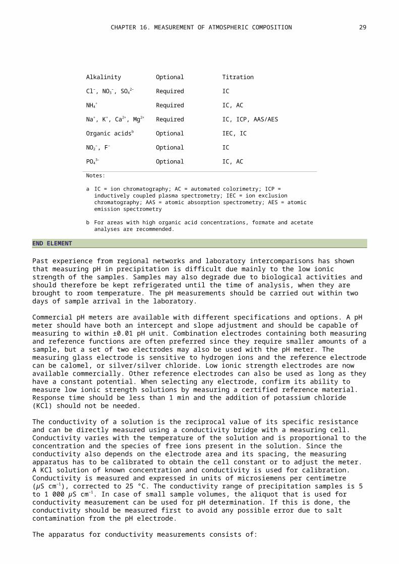
CHAPTER 16. MEASUREMENT OF ATMOSPHERIC COMPOSITION 29
Variable Frequency of observation
Aerosol number concentration Continuous
Aerosol number size distribution Continuous
Cloud condensation nuclei number concentration at various supersat-urations
Continuous
Vertical distribution of aerosol backscattering and extinction Continuous
Detailed size fractionated chemical composition Intermittent
Dependence of aerosol variables on relative humidity, especially aero-sol number size distribution and light scattering coefficient
Intermittent
Source: WMO (20116b)
16.6.1 Aerosol chemical measurements
At present, filter collection of ambient aerosol, followed by laboratory analyses, still remains the most commonly used and cost-efficient method for the determination of aerosol chemical composi-tion despite well-documented artefacts. Artefacts are very often linked to the presence of semi-volatile species that can either condense upon sampling (positive artefact) or evaporate from the filter media after sampling (negative artefact). A number of methods have been proposed to limit these artefacts, but none of them will satisfactorily apply to all chemical substances present in aerosol.
The optimal set-up for the characterization of chemical properties of aerosol would be composed of a series of denuders to remove condensable species present in the gas phase (limiting positive artefact) and a filter pack collecting both particles and condensable species re-emitted from the first filter (accounting for negative artefact). Filter packs have been developed, consisting of a sandwich of filters and collection media of various types in series, to collect aerosols and select-ively trap gases and aerosol volatilization products. Ideally, sampling for inorganic and carbon-aceous species is performed with two different sampling lines since different kinds of denuders and filter media are required for analyses of elemental and organic carbon (EC/OC), and inorganic species. A third line could be implemented for sampling and analysis of elemental aerosol compos-ition.
Clearly, methods for artefact limitation can be rather impractical and are relatively expensive. For GAW purposes, considering remoteness and the availability of resources in a number of sites, the use of denuders should be seen as a simple recommendation and not a requirement. This means, however, that sampling artefacts do exist for a number of semi-volatile species, in particular when temperatures in the sampling system exceed 20 °C. This should be accounted for when reporting data to the World Data Centre for Aerosols.
High-volume and low-volume sampling lines are accepted in the context of GAW. For simplicity, it is suggested that a differencing technique be utilized to separate the coarse fraction from the fine fraction. Specifically, one filter should be run behind the 10 µm aerodynamic diameter cut inlet. A parallel filter should be run behind the inlet suitable for the fine fraction (i.e. 2.5 µm aerodynamic diameter at ambient relative humidity or 1.0 µm in dry air). While the second filter will yield the fine fraction, the difference between the two filters will yield the coarse fraction. For high-volume sampling, use of dichotomous samplers is an interesting alternative to differentiate fine and coarse aerosol fractions.
Low-volume samplers are more easily implemented than high-volume samplers. For the routine long-term aerosol measurements at GAW stations, it is recommended that up to three sets of 47 mm diameter filters be collected in parallel by low-volume samplers. If financial constraints are
30 PART I. MEASUREMENT OF METEOROLOGICAL VARIABLES
limiting, the priorities for filter sampling are: (i) Teflon filters for gravimetric and ionic analyses; (ii) quartz-fibre filters for carbonaceous aerosol analyses; and (iii) Teflon filters for elemental analyses. Each set would consist, ideally, of two filters, one for total mass below 10 µm diameter and one for the fine fraction. The separation would be achieved by running the filters behind the size-selective inlets. High-volume samplers are usually more expensive, and running more than one set of sampler in parallel is often unpractical. For that reason, it is recommended that high-volume samplers be operated with quartz fibre filters for both inorganic and EC/OC analyses. It should be noted that denuders for high-volume samplers are not commercially available.
There is no recommendation for determining sampling time as this will highly depend upon the sites. In general, short sampling time (24 to 48 h) provides information that is more easily used in models and should be preferred over week-long sampling, even if discontinuous. Filters should be removed from the sampling unit shortly after collection and stored between 0 °C and 5 °C if ana-lyses cannot be performed immediately. Regular blanks should be performed in order to control for contamination. Ideally, blanks are prepared by mounting filters into the sampling unit with the pump off. We recommend that one blank be performed every 10 samples.
For each GAW aerosol station, a list of core aerosol chemical measurements is strongly recommen-ded: (i) mass; (ii) major ionic species; (iii) carbonaceous components, and (iv) dust aerosols.
The mass concentration of atmospheric aerosols is clearly a fundamental parameter in the GAW measurement programme. It is recommended that this be done gravimetrically on Teflon filters. It is expressed in units of µg m–3, where the volume is related to STP. Updated measurement guidelines on mass concentration measurements using gravimetric analysis of Teflon filters are provided in WMO (2011c).
The tapered element oscillating microbalance (TEOM) has been widely used for aerosol mass measurements. The instrument provides continuous measurements and can produce high time resolution data. The original TEOM has a recommended temperature setting of 50 °C. There is evidence that semi-volatile components of aerosols are lost from the TEOM measurements at this temperature. The most likely explanation is that semi-volatile organic compounds, nitrates and water are lost from the aerosols during sampling. In newer TEOM models, the operating temperat-ure has been lowered to 30 °C to reduce losses of the semi-volatile components. In addition, sud-den changes in ambient relative humidity may cause negative mass readings from the instrument. New modifications have been made to dry the aerosol particles before measurement to reduce the effect of ambient relative humidity.
A different type of instrument for continuous mass measurements, the β-meter, has also been commercialized. It operates on the principle of β-ray attenuation by a layer of aerosol. The β-ray source is usually 14C or 85Kr decay, and the attenuation can be calibrated with a known mass. Sampling can be done with individual filters or filter tapes, and the β-ray that passes through the filter is continuously monitored. The β-meters have the same inherent difficulties concerning volat-ilization as the TEOM. However, comparison with gravimetric methods usually produces reasonable agreement. Updated guidelines on the mass concentration measurements with beta attenuation (with the Met One Instruments model BAM-1020) are provided in WMO (2011c).
The concentration of major inorganic species is one of the core pieces of information recommen-ded for the GAW stations. Major ionic species include sulphate, nitrate, chloride, sodium, am-monium, potassium, magnesium and calcium. This selection is based on the fact that analytical procedures for these species have become well established. More importantly, under most atmo-spheric conditions, this set of ions is expected to account for a major part of the aerosol mass, and the measurements here are an important step towards mass closure of the aerosols. As mentioned above, quantitative measurements of nitrate with a filter technique remain problematic and are associated with high uncertainties.
In the GAW Programme, it is recommended that analyses be done using ion chromatography for the most cost-effective approach. The IC technique has the advantage of chemical speciation and relatively low cost per analysis, and has matured to the degree that the sensitivities for each ionic
CHAPTER 16. MEASUREMENT OF ATMOSPHERIC COMPOSITION 31
species, the cost and the maintenance are all reasonably well known. If IC is set up properly, all the recommended ionic species can be analysed in one single sample injection. Alternative analyt-ical techniques exist but their use may introduce systematic differences among GAW stations. It is part of each laboratory’s responsibility to document the equivalence of these alternative tech-niques, such as AAS or ICP-MS, with IC whenever they are used. Calibration of IC instruments is an integral part of every laboratory’s standard operating procedures, and each laboratory must imple-ment quality control procedures that guarantee the accuracy of calibrations. Recommendations for GAW are similar to those reported in WMO (2004b) for precipitation chemistry. In addition, proto-cols for filter extraction should be well documented.
Instruments are emerging on the scene for continuous and semi-continuous measurement of sulphate, nitrate, and organic carbon in aerosols. In particular, progress in aerosol mass spectro-metry (AMS) has led to the development of instruments that can be used for monitoring purposes, providing quantitative measurements of the total mass and size distribution of non-refractory chemical composition in the submicron-size range. For example, the aerosol chemical speciation monitor (ACSM) is a simple version of AMS that can provide chemically speciated mass loadings and aerosol mass spectra with one-hour time resolution. No standard operating procedures exist yet for ACSM or other AMS instruments, but the method’s suitability for long-term monitoring is clear and will undoubtedly bring revision of aerosol chemical speciation procedures in the future.
The concentration of carbonaceous species (with both elemental and organic fractions) is also one of the core pieces of information recommended at GAW stations. Carbonaceous species are still the least understood and most difficult to characterize of all aerosol chemical components. Total aerosol carbon mass can be divided into three fractions: inorganic carbonates, organic carbon (OC), and a third fraction ambiguously called elemental carbon (EC), black carbon (BC), soot or refractory carbon in the scientific literature with no clear definition of the terms. Recommendations for proper use of terminology for BC-related species have been proposed by Petzold et al. (2013) to clarify the terms used in atmospheric research; they recommend that the term “black carbon” be used only in a qualitative sense, and that terms related to the measurement technique be used when reporting quantitative results. According to this terminology, thermo-optical methods can be used to derive total carbon (TC) and OC/EC fraction in atmospheric aerosol filters. When using op-tical methods, the light-absorbing component is called equivalent black carbon (EBC), even though the optical method is not specific for carbon.
It is recommended that TC, OC and EC be measured in the GAW Programme, leaving out the relat-ively minor and difficult inorganic carbon component and the more complicated issue of organic carbon speciation. Sampling of aerosol carbonaceous materials is recommended using quartz fil-ters, pre-fired at 350 °C to 400 °C for 2 h, and at the same sampling frequency as the Teflon fil-ters. The quartz filter can be analysed for TC using the thermal evolution technique. The mass con-centration of the total carbon is obtained by thermal oxidation of the carbon, usually at 750 °C in the presence of a catalyst, to measurable carbon dioxide. Detection of the evolved carbon dioxide is done in one of two ways: either by reduction to methane in the presence of a catalyst, and then FID, or by direct detection by NDIR detectors.
The measurement of the TC components – OC and EC – is more difficult than the measurement of TC (Schmid et al., 2001). The distinction between the fractions is made by temperature-controlled volatilization/pyrolysis. This is followed by catalysed oxidation to CO2 and detection by NDIR, or in some instruments, further catalysed reduction of the CO2 to CH4 and final detection by FID. There are different temperature-control programmes in use. At present, GAW recommends the use of one of three thermo-optical techniques: the IMPROVE (Interagency Monitoring of Protected Visual Environments) protocol (Chow et al., 1993; Chow et al., 2005), NIOSH (National Institute for Occu-pational Safety and Health) protocol (Birch and Cary, 1996) and EUSAAR-2 (European Supersites for Atmospheric Aerosol Research) protocol (Cavalli et al., 2010). Relatively good agreement is obtained between the IMPROVE, NIOSH and EUSAAR-2 protocols for TC determination, while they strongly differ for EC determination (Chow et al., 2001). Because EC represents a relatively small fraction of TC, OC determination by the three protocols is also comparable. It is accepted that the IMPROVE and EUSAAR-2 protocols are most suited for non-urban background sites, while the NIOSH is applied to samples from urban sites in the US Environmental Protection Agency (EPA).

32 PART I. MEASUREMENT OF METEOROLOGICAL VARIABLES
The use of IMPROVE or EUSAAR-2 may therefore be preferred over NIOSH for global remote GAW stations. Use of the EUSAAR-2 and IMPROVE protocols for EC determination may lead to different results but should be preferred over any alternative techniques. Whenever an alternative approach is used for OC measurements, it is recommended that a periodic determination of OC using one of the thermo-optical methods be conducted so that results can be compared. This is also true for AMS techniques before a standardized protocol is well established.
The use of optical methods for estimating EBC involves measuring the change in optical transmis-sion of a deposit of particles on a filter (absorption) and applying a site-specific and instrument type-specific mass absorption efficiency to derive EBC. Two key assumptions are required to de-rive the equivalent black carbon mass concentration from light absorption measurements: (i) black carbon is the only species responsible for the aerosol light absorption, and (ii) the sampled black carbon has the same mass absorption efficiency as the standards used in laboratory calibrations of the absorption instrument. These assumptions can be evaluated by experimentally determining the mass absorption efficiency by simultaneously making light absorption measurements and EC measurements as described above. At sites where EC concentrations are not routinely determined on quartz-fibre filters, less frequent filter collections can be used to derive site- and season-specific values of the mass absorption efficiency. Thus, for GAW measurements of EBC, experimentally derived values of the mass absorption efficiency at a site are essential when estimating black car-bon mass concentration from light absorption measurements.
The use of incandescent methods, such as single-particle soot photometers, or volatility tech-niques, such as volatility scanning mobility particle sizer (SMPS), can provide information on re-fractory material present in aerosol, but their use in monitoring activities at GAW stations remains problematic given the lack of standardized protocols and of consistent intercomparison with thermo-optical techniques.
Dust aerosols can be sampled relatively easily without the problems posed by more semi-volatile aerosol components such as organics and ammonium nitrate. For GAW stations, it is recommen-ded that a multi-elemental analysis approach be used to determine the mineral dust component. Teflon filters should be analysed for at least four of the major crustal elements, aluminium (Al), silicon (Si), iron (Fe), titanium (Ti) and scandium (Sc), and the related elements, sodium (Na), mag-nesium (Mg), potassium (K) and calcium (Ca). No specific analytical technique is recommended as there is a good selection available, including proton-induced X-ray emission (PIXE), instrumental neutron activation analysis (INAA), X-ray fluorescence (XRF), AAS and ICP-MS. These techniques usually have high sensitivities for the crustal elements. Not all techniques can provide all the re-quired elements, and depending on availability, a combination of two or more techniques may be necessary.
16.6.2 In situ measurements of aerosol radiative properties
The following aerosol radiative properties are needed for climate studies, all at multiple wavelengths across the visible spectrum:
(a) The aerosol light extinction coefficient (ep) and its two components (scattering and absorption).
(b) The aerosol optical depth (δ, see 16.6.5), defined as the integral over the vertical column of the aerosol light extinction coefficient.
(c) The aerosol single-scattering albedo (o), defined as sp/(ap + sp), describes the relative contributions of scattering and absorption to the total light extinction. Purely scattering aerosols (such as sulphuric acid) have values of 1, while very strong absorbers (such as black carbon) have values of about 0.3.
(d) Radiative transfer models commonly require one of two integral properties of the angular distribution of scattered light (phase function): the asymmetry factor (g) or the upscatter fraction (β). The asymmetry factor is the cosine-weighted average of the phase function,
CHAPTER 16. MEASUREMENT OF ATMOSPHERIC COMPOSITION 33
ranging from a value of –1 for entirely backscattered light to +1 for entirely forward-scattered light. The upscatter fraction gives the fraction of sunlight scattered in the upwards direction (back to space), which depends on the solar zenith angle as well as the size distribution and chemical composition of the particles. It can be estimated from the hemispheric backscatter fraction (b).
(e) The mass scattering efficiency for species i, (si), is used in chemical transport models to evaluate the radiative effects of each chemical species forecast by the model. It is often calculated as the slope of the linear regression line relating the aerosol light scattering coefficient (sp) and the mass concentration of the chemical species (though multiple linear regression is preferred, to deal with covariance of some chemical species). This parameter has units of m2 g–1.
(f) The mass absorption efficiency for species i, (ai), is used in chemical transport models to evaluate the radiative effects of each chemical species forecast by the model. It is often calculated as the slope of the linear regression line relating the aerosol light absorption coefficient (ap) and the mass concentration of the chemical species (though multiple linear regression is preferred, to deal with covariance of some chemical species). This parameter has units of m2 g–1.
(g) The functional dependence of components of the aerosol light extinction coefficient (ep, sp, ap) on relative humidity, f(RH), expressed as a multiple of the value at a low reference relative humidity (typically < 40%).
The aerosol light scattering coefficient is measured with an integrating nephelometer. Integrating nephelometers have been operated at baseline monitoring stations since the deployment of a four-wavelength instrument at the NOAA Mauna Loa Observatory in 1974. At present, there are about four dozen sites monitoring sp routinely around the globe as part of the GAW global net-work. A few of these are operating single-wavelength units, but most are measuring sp at three wavelengths. The multiwavelength integrating nephelometer TSI model 3563 operates at wavelengths of 450, 550 and 700 nm, and has the added feature of being able to measure sp over two angular ranges: total scattering (7°–170°) and hemispheric backscattering (90°–170°, denoted as bsp). The Aurora 3000 integrating nephelometer, manufactured by Ecotech, makes comparable measurements. While instruments do not exist for direct determination of g or β, the ratio b = bsp/sp can be used to estimate either of these parameters (updated measurement guidelines are available in WMO (2011c)). Simpler, less expensive and less sensitive one-wavelength instru-ments are also commercially available. These instruments can provide useful information on the aerosol light scattering coefficient at regional sites where aerosol loadings allow the use of a less sensitive instrument.
Instruments capable of high time-resolution determination of the aerosol light absorption coeffi-cient are commercially available. They are based on the rate of change of transmission through a fibre filter as particles are deposited on the filter. Calibration of these filter-based methods is diffi-cult but required because the relationship between the change in light transmission and aerosol absorption optical depth on the filter depends on many factors, including the particular filter me-dium and the light-scattering nature of the particles.
One instrument in common use is the aethalometer. Originally, this instrument was calibrated in terms of an equivalent mass of black carbon rather than the fundamental property that provides the instrumental response: aerosol light absorption. Early models of the aethalometer have a very broad wavelength response, while newer versions offer narrowband measurements at multiple wavelengths.
Another commercial, filter-based instrument for determining ap is the particle soot absorption pho-tometer (PSAP) that measures laboratory aerosols with different single-scattering albedos, using a calibration standard based on the difference between ep, measured with a long-path extinction cell, and sp, measured with an integrating nephelometer. Updated measurement guidelines for PSAP instruments are provided in WMO (2011c).
34 PART I. MEASUREMENT OF METEOROLOGICAL VARIABLES
Yet another filter-based instrument is the multi-angle absorption photometer (MAAP). The MAAP uses a different optical configuration than the aethalometer and PSAP, with measurements of the filter reflectivity at two different angles in addition to the filter transmission measurement. The two reflectivity measurements allow correction for multiple scattering processes involving the depos-ited particles and the filter matrix. This approach eliminates the need for a correction scheme based on independent measurements of the aerosol light scattering coefficient. The MAAP oper-ates at a wavelength of 670 nm. Updated measurement guidelines for MAAP instruments are provided in WMO (2011c).
Recent improvements in a different approach to determining the aerosol light absorption coeffi-cient, called photoacoustic spectroscopy, offer a promising alternative to filter-based methods. Although not as sensitive, the photoacoustic method allows determination of the aerosol light ab-sorption coefficient while the particles are suspended in air, eliminating the artefacts introduced by depositing the particles on a filter. The photoacoustic method can be used in regions where light absorption levels are moderately high, and as a calibration standard for filter-based instru-ments.
16.6.3 Particle number concentration and size distribution
Condensation nuclei (CN) can be detected after the condensation of water or other condensable vapour (often an alcohol such as butanol) from a supersaturated atmosphere onto the particle. The supersaturation in condensation nuclei counters (CNCs), which are also known as condensation particle counters (CPCs), is typically quite large, about 150%, allowing the detection of particles as small as a few nanometres in diameter.
Optical methods are usually used to detect the resulting droplets. Early counters relied on manual counting, either in situ or after photography. The Nolan-Pollak counter and its derivatives (such as the Gardner counter) rely on determination of the optical extinction of the resulting cloud. Photo-metric observation of light scattered by the droplets is used in some counters. The most satisfact-ory method is individual counting of particles condensed in a continuous flow, as employed in the family of CNCs that have developed from the design of Bricard et al. (1976). This procedure is em-ployed in most modern commercial CNCs. It has the advantage of giving a direct determination of CN concentrations up to about 105 cm–3 (although this limit is not generally reached by simpler, lower-cost counters).
Because of the complexity of the particle number size distribution measurement, it is recommen-ded that number size distribution determinations be undertaken only at GAW stations with more highly developed aerosol programmes. Many commercial instruments are available to do this. They utilize a wide range of physical principles to classify particles according to size. Some of the better-known approaches use the electrical mobility of particles, aerodynamic size, or optical size determined by light scattering. This latter class includes a number of relatively small, low-cost in-struments utilizing laser diodes. While any of these measurement approaches has the potential to add useful data to the overall GAW aerosol measurement programme, it is assumed that stations operating such instrumentation will have a highly developed aerosol programme that includes doc-umentation, calibration and quality control measures.
16.6.4 Cloud condensation nuclei
Cloud condensation nuclei (CCN) measurements are made to determine the concentration and establish climatologies of those particles that have the potential to produce cloud droplets at su-persaturations typical of natural clouds, that is, less than about 1%. Because of the complexity of the measurement, it is recommended that CCN determinations be undertaken at GAW stations with more highly developed aerosol programmes. Past CCN measurements in the GAW Programme have been made predominantly using static thermal-gradient chambers, which are well suited to relatively low-frequency sampling and low-resolution (differential) CCN spectrum determination. Instruments utilizing continuous flow offer another approach, and a commercial instrument using this approach is being deployed at a growing number of GAW stations. Measurement methods that have available droplet growth times comparable to real clouds are preferable.
CHAPTER 16. MEASUREMENT OF ATMOSPHERIC COMPOSITION 35
16.6.5 Aerosol optical depth
Aerosol optical depth (AOD) is retrieved from observations of atmospheric spectral transmission. The solar spectral irradiance I at a given wavelength can be expressed as:
(16.3)
with I0 being the extraterrestrial (top of the atmosphere) irradiance of the sun, m the optical air-mass and δ the total optical depth. The optical airmass equals 1 for a vertical path through the atmosphere and is roughly proportional to 1/cos z, with z being the zenith angle of the sun during the observation. The total optical depth δ at a given wavelength is composed of several compon-ents, such as scattering by gas molecules δR (Rayleigh scattering), extinction by aerosol particles δA, absorption of trace gases δG (ozone, nitrogen dioxide, etc.), and possible cloud contamination. Thus, the AOD can be obtained from the total optical depth by subtracting modelled estimates of the other components δA = δ – δR – δG.
Because AOD is essentially a difference between two larger numbers, it is sensitive to small calib-ration errors and, to a minor degree, to the methods chosen to model the other components. A traceable calibration uncertainty of 1.5%, corresponding to an uncertainty of 0.015 optical depths at unit optical airmass, should be maintained for AOD observations (WMO, 2005).
Wavelengths and bandpasses specifically for AOD that are largely free of variable extinction com-ponents (water vapour and NOx) and strong ozone extinction have been recommended in WMO (2003a2003). The Baseline Surface Radiation Network (BSRN) and GAW-PFR (a network of aerosol optical depth observations with precision filter radiometers) are using four AOD channels at 368, 412, 500 and 862 nm. While some other networks have selected different wavelengths based on their specific needs (validation of satellite sensors, modelling efforts), measurements at 500 ±3 nm and 865 ±5 nm are typically available in most networks.
Measurements of the solar spectral irradiance are traditionally taken by sun-pointing radiometers (sun photometers) mounted on a two-axis solar tracker, with a sampling rate of once every minute to allow for objective quality control and cloud filtering algorithms. Homogeneous quality control is more difficult to achieve with handheld sun photometers.
Rotating shadow-band filter radiometers measure global and diffuse spectral irradiance at several wavelength bands. Direct normal irradiance obtained as the difference between global and diffuse radiation, normalized by the solar zenith angle, can be used to retrieve AOD the same way as with sun photometers.
More advanced instruments like sky-scanning radiometers can be used to infer additional column aerosol optical properties, including size distribution, single-scattering albedo or phase function, through sophisticated mathematical inversion models.
Sun photometers and shadow-band and sky-scanning radiometers are commercially available from several manufacturers. Centralized data evaluation and calibration services6 are offered for stand-ardized instruments by global networks, such as the Aerosol Robotic Network (AERONET), GAW-PFR or SKYNET (WMO, 2005).
16.6.6 GAW aerosol lidar
The basic lidar principle is the following: a laser pulse is transmitted into the atmosphere where it encounters gas molecules and particles; a small amount of this energy is backscattered in the dir-ection of the receiver system, typically a telescope, and transferred to a photodetector as a pho-tomultiplier. The resulting electrical signal is proportional to the optical power received, which de-pends on the presence, range and concentration of atmospheric scatterers and absorbers in the
6 For more details, see the World Optical Depth Research and Calibration Centre website (at http://www.pmodwrc.ch/worcc/index.html).

36 PART I. MEASUREMENT OF METEOROLOGICAL VARIABLES
light path volume. Lidar techniques are able to characterize atmospheric aerosols in terms of ver-tical profiles of extinction and backscatter coefficients, lidar ratio, optical depth and microphysical properties such as shape, refractive index and size distribution, on timescales as short as minutes and vertical scales as short as metres.
Lidar observations are much more powerful if used in coordinated networks. Lidar networks are fundamental to studying aerosols on a large spatial scale and to investigating transport and modi-fication phenomena. There are several research lidar networks that contribute to GAW: the Asian Dust and Aerosol Lidar Observation Network (AD-NET), Latin American Lidar Network (LALINET or ALINE), Commonwealth of Independent States Lidar Network (CIS-LINET), European Aerosol Re-search Lidar Network (EARLINET), Micro Pulse Lidar Network (MPLNET), NDACC, and the NOAA Co-operative Remote Sensing Science and Technology (CREST) Lidar Network. These networks are coordinated within the GAW Aerosol Lidar Observation Network (GALION; WMO, 2008b).
Several different lidar techniques exist, depending on the specific instrument design and mainly on the specific laser-atmosphere scattering process.
Elastic backscatter lidar
This is the simplest type of aerosol lidar: the backscattered wavelength is identical to the transmit-ted wavelength, and the magnitude of the received signal at a given range depends on the backs-catter cross-section of scatterers along the path to that range. Typical operating wavelengths are 355, 532 and 1 064 nm. The typical product of a backscatter lidar is the vertical profile of the aero-sol backscatter coefficient obtained assuming a lidar ratio, i.e. the extinction-to-backscatter ratio, that is mostly constant throughout the profile and usually derived from an existing climatology obtained with measurements from a Raman lidar, described later. In this sense, it is necessary to underline that without an a priori assumption about the lidar ratio, this kind of lidar system cannot provide quantitative aerosol backscatter data.
Depolarization lidar
These are elastic backscatter lidars equipped with channels for the detection of the two parallel and cross-polarized components of the backscattered radiation. This provides quantitative inform-ation about particle shape, strongly contributing to aerosol typing as well as to the identification of thin clouds contaminating the profiles. A depolarization channel allows discrimination of volcanic ash and other aerosol particles. Typical operating wavelengths are 355 and 532 nm. Depolariza-tion lidar systems need accurate calibration.
Raman lidar
The Raman lidar technique operates by measuring the inelastic Raman scattering by a specific gas. The Raman backscattered radiation from molecular nitrogen (or oxygen) is typically used for retrieving the vertical profile of the aerosol extinction coefficient that, coupled with the elastic scattering collected at the same emission wavelength, provides also the vertical profile of the aer-osol backscatter coefficient without assuming a lidar ratio. Typical operating wavelengths are 355 and 532 nm. Most of the existing Raman lidar instruments are also equipped with a depolarization channel providing data on the particle linear depolarization ratio. Advanced multiwavelength Ra-man aerosol lidar techniques have been demonstrated to be the only technique capable of provid-ing range-resolved aerosol microphysical properties. Moreover, rotational Raman lidar systems can be designed for optimizing extinction measurements in daytime conditions.
High spectral resolution lidar
The high spectral resolution lidar (HSRL) technique provides calibrated measurements of aerosol optical depth, extinction and backscatter. Measurements are computed from ratios of the particu-late scattering to the measured molecular scattering. This provides absolute calibration and makes the calibration insensitive to dirt or precipitation on the output window. A very narrow, angular field-of-view reduces contamination from spurious sources, like multiple scattering contributions.

CHAPTER 16. MEASUREMENT OF ATMOSPHERIC COMPOSITION 37
The small field-of-view, coupled with a narrow optical bandwidth, nearly eliminates noise due to scattered sunlight, improving the signal-to-noise ratio also during daytime operations.
Ceilometers
Ceilometers are basically elastic backscatter lidars that employ a diode laser source emitting at infrared wavelengths (typically 905 or 1 064 nm) using a low energy but a high repetition rate (in units of µJ of energy per pulse and kHz for the rate) and that detect the elastic backscattered radi-ation by clouds and precipitation. Ceilometers are a self-contained, turnkey, surface-based, active, remote-sensing device designed to measure cloud-base height and potentially the backscatter signals by aerosols. Ceilometers can provide qualitative information about aerosol vertical distribu-tion. Generally, older and typically less powerful instruments are barely able to detect aerosol lay-ers in the atmosphere, while newer instruments are quite useful for volcanic ash/dust detection and ash/dust plume tracking.
All of these lidar techniques can provide data products suitable for monitoring the spatial and tem-poral distribution of aerosol up to the upper troposphere/lower stratosphere region and can char-acterize them from a dynamical and microphysical point of view. The main lidar limitation is re-lated to the presence of rain, dense fog and thick clouds (optical depths larger than 2–3) that do not allow monitoring of the atmosphere above the cloud-base region. The altitude range covered by lidars is limited at the bottom by the overlap height (altitude where there is a full overlap between the transmitter and the receiver) that is typically about 250–500 m above the ground level but could be also up to 2 km above the ground depending on the specific design. The max-imum altitude range strongly depends on the laser power and optical design, but can be up to 25–30 km for high-power systems. It is difficult to provide general estimates of the accuracy of the different lidar products because these strongly depend on the specific system and on the meteoro-logical conditions. On average, uncertainties for extinction and backscatter coefficient are about 20% (in the case of Raman lidar or HSRL). The retrieval of microphysical properties is possible only if optical data have uncertainties lower than 20%–30%.
Aerosol lidar products (see Table 16.4 for more details):
(a) Geometrical properties:
(i) Layer identification (top, bottom and centre of mass);
(b) Profiles of optical properties:
(i) Extensive optical parameters: aerosol backscatter coefficient (a), aerosol extinction coefficient (a);
(ii) Intensive optical parameters: lidar ratio, particle linear depolarization ratio (δa), Ångström backscatter-related exponent (Å), Ångström extinction-related exponent (Å);
(c) Optical properties in the identified layer:
(i) Integrated backscatter, aerosol optical depth;
(ii) Mean intensive optical parameters (lidar ratio, particle linear depolarization ratio, Ångström backscatter-related exponent, Ångström extinction-related exponent);
(d) Aerosol typing classification;
(e) Mass concentration estimate;
(f) Microphysical properties retrieved.
38 PART I. MEASUREMENT OF METEOROLOGICAL VARIABLES
Table 16.4. Lidar products related to specific surface-based lidar techniques(note that (d) = daytime only)
TABLE: Table horizontal lines
Surface-based lidar techniques
Geometrical properties βa a
Lidar ratioa AOD Åβ Å Type b Microphysical
properties
Ceilometerc ✓ ✓ d
Ceilometer + sun photometer
✓ ✓ ✓(d)f ✓(d)
Ceilometer + sun photo. + depolarization lidar
✓ ✓ ✓(d)f ✓(d) ✓(limited)
1-wavelength (1-λ) backscatter lidar
✓ ✓
1-λ backscatter lidar + sun photometer
✓ ✓ ✓(d)f ✓(d)
1-λ backscatter lidar + sun photo. + depolarization lidar
✓ ✓ ✓(d)f ✓(d) ✓(d) (limited)
Multiwavelength (m-λ)e backscatter lidar
✓ ✓ ✓
M-λe backscatter lidar + sun photometer
✓ ✓ ✓(d)f ✓(d) ✓(d)f ✓ ✓(d)f
M-λe backscatter lidar + sun photo. + depolarization lidar
✓ ✓ ✓(d)f ✓(d) ✓(d)f ✓ ✓ ✓(d)f
1-λ Raman lidar/HSRL ✓ ✓ ✓ g ✓ g ✓ g ✓ g (limited)
1-λ Raman lidar/HSRL + sun photometer
✓ ✓ ✓ g ✓ g ✓ g ✓(d)f ✓(d)f ✓(limited)
✓(d)f
1-λ Raman lidar/HSRL + sun photo. + depol-arization lidar
✓ ✓ ✓ g ✓ g ✓ g ✓(d)f ✓(d)f ✓ ✓(d)f
M-λe Raman lidar ✓ ✓ ✓ g ✓ g ✓ g ✓ g ✓ ✓ g ✓ g
M-λe Raman lidar + sun photometer
✓ ✓ ✓ g ✓ g ✓ g ✓ g ✓ ✓ ✓ g
M-λe Raman lidar + sun photo. + depolarization lidar
✓ ✓ ✓ g ✓ g ✓ g ✓ g ✓ ✓ ✓ g
Notes:
a From two independent measurements
b Identification of scattering type (aerosol particles, cloud droplets, ice crystals, some aerosol type information)
CHAPTER 16. MEASUREMENT OF ATMOSPHERIC COMPOSITION 39
c A ceilometer is a single-wavelength, low-power lidar, with lower signal-to-noise ratio.
d If calibrated
e m > 2
f Estimate only
g Most Raman lidar systems operate during night-time. Some 24-h Raman lidar systems exist and their operability has been proved. However, few systems nowadays operate Raman channels also during daytime; HSRL is independent of daytime.
16.7 NATURAL RADIOACTIVITY
The global distributions of the source/sink terms of the naturally occurring radionuclides (7Be, 10Be, 210Pb and 222Rn) and the anthropogenic radionuclides (85Kr) are reasonably well known. 7Be and 10Be are produced by cosmic-ray interactions in the upper troposphere and lower stratosphere. 222Rn is exhaled from the Earth’s land surface as a result of uranium decay in soil. 210Pb is produced in the lower troposphere from the decay of 222Rn. Most of the 85Kr in the atmosphere is released during nuclear fuel reprocessing. Atoms of 7Be, 10Be and 210Pb attach themselves to submicron-size aero-sol particles, and therefore act as aerosol-borne tracers in the atmosphere. 222Rn and 85Kr, which are chemically and physically inert, act as noble gases in the atmosphere.
Measurements of radionuclides are not a priority area within the GAW Programme. Some general recommendations can be found in WMO (2001) and WMO (2004a).
SECTION: Chapter_book
Chapter title in running head: CHAPTER 16. MEASUREMENT OF ATMOSPHERIC …
Chapter_ID: 8_I_16_en
Part title in running head: PART I. MEASUREMENT OF METEOROLOGICAL VARI…
ANNEX. GAW CENTRAL FACILITIES
List of GAW central facilities and host institutions as of September 2013; the World Central Facilities have assumed global responsibilities, unless indicated.
TABLE: Table horizontal lines
VariableQuality
Assurance/Science Activity Centre
Central Calibration Laboratory
(host of primary standard)
World Calibration Centre
Regional Calibra-tion Centre
World Data Centre
CO2 JMA (A/O)a NOAA-ESRL NOAA-ESRL (round robin)Empa (audits)
JMA
Carbon isotopes MPI-BGC JMA
CH4 Empa (Am, E/A)a
JMA (A/O)aNOAA-ESRL Empa (Am, E/A)a
JMA (A/O)aJMA
40 PART I. MEASUREMENT OF METEOROLOGICAL VARIABLES
N2O UBA NOAA-ESRL IMK-IFU JMA
CFCs, HCFCs, HFCs JMA
SF6 NOAA-ESRL KMA JMA
H2 MPI-BGC JMA
Total ozone JMA (A/O)a NOAA-ESRL,b ECc NOAA-ESRL,b ECc BoM,b NOAA-ESRL,b IZO,c JMA,b MOHp,b MGO,d OCBA,b SAWS,b SOO-HKb
EC,f DLRg
Ozonesondes IEK-8 IEK-8 IEK-8 EC
Surface ozone Empa NIST Empa OCBA JMA
Precipitation chem-istry
NOAA-ARL ISWS ISWS NOAA-ARL
CO Empa NOAA-ESRL Empa JMA
VOCs UBA NPL, NIST, KRISS IMK-IFU JMA
SO2 JMA
NOx UBA IEK-8 (NOx) JMA
Aerosol UBA (physical prop-erties)
TROPOS (physical properties)
NILU,f DLRg
Optical depth PMOD/WRCe PMOD/WRC NILU
UV radiation PMOD/WRC NOAA-ESRL (Am),a EUVC/PMOD (E)a
EC
Solar radiation PMOD/WRC PMOD/WRC MGO
Notes:
a Am = Americas; E/A = Europe and Africa; A/O = Asia and the South-West Pacific
b Dobson
c Brewer
d Filter instruments
e Precision filter radiometers
f Surface-based
g Space-based
Host institutions
TABLE: Table as text NO space
BoM Bureau of Meteorology, Melbourne, Australia
BSRN Baseline Surface Radiation Network, Federal Institute of Technology (ETH), Zürich, Switzerland
DLR German Aerospace Centre, Oberpfaffenhofen, Wessling, Germany
CHAPTER 16. MEASUREMENT OF ATMOSPHERIC COMPOSITION 41
EC Environment Canada, Toronto, Canada
Empa Swiss Federal Laboratories for Materials Testing and Research,Dübendorf, Switzerland
EUVC European Ultraviolet Calibration Centre (see PMOD/WRC)
IEK-8 Institute of Energy and Climate Research: Troposphere (IEK-8), Research Centre Jülich GmbH, Jülich, Germany
TROPOS Institute for Tropospheric Research, Leipzig, Germany
IMK-IFU Karlsruhe Institute of Technology (KIT), Institute of Meteorology and Climate Research – Atmospheric Environmental Research, Garmisch-Partenkirchen, Ger-many
ISWS Illinois State Water Survey, Champaign, IL, United States
IZO Izaña Observatory, Tenerife, Spain
JMA Japan Meteorological Agency, Tokyo, Japan
KMA Korea Meteorological Administration, Seoul, the Republic of Korea
KRISS Korea Research Institute of Standards and Science, Daejeon, the Republic of Korea
MGO A.I. Voeikov Main Geophysical Observatory, Russian Federal Service for Hydro-meteorology and Environmental Monitoring, St. Petersburg,the Russian Federation
MPI-BGC Max Planck Institute for Biogeochemistry, Jena, Germany
MOHp Meteorologisches Observatorium Hohenpeissenberg, Hohenpeissenberg, Germany
NOAA-ARL National Oceanic and Atmospheric Administration, Air Resources Laboratory, Silver Spring, MD, United States
NOAA-ESRL National Oceanic and Atmospheric Administration, Earth System Research Laboratory, Global Monitoring Division, Boulder, CO, United States
NILU Norwegian Institute for Air Research, Kjeller, Norway
NIST National Institute of Standards and Technology, Gaithersburg, MD, United States
NPL National Physical Laboratory, Teddington, Middlesex, United Kingdom
OCBA Observatorio Central de Buenos Aires, Argentina
PMOD/WRC Physikalisch-Meteorologisches Observatorium Davos/World Radiation Centre, Davos, Switzerland
SAWS South African Weather Service, Pretoria, South Africa
SOO-HK Solar and Ozone Observatory, Hradec Kralove, Czech Republic
UBA German Environmental Protection Agency, Berlin, Germany

42 PART I. MEASUREMENT OF METEOROLOGICAL VARIABLES
SECTION: Chapter_book
Chapter title in running head: CHAPTER 16. MEASUREMENT OF ATMOSPHERIC …
Chapter_ID: 8_I_16_en
Part title in running head: PART I. MEASUREMENT OF METEOROLOGICAL VARI…
REFERENCES AND FURTHER READING
Birch, M.E. and R.A. Cary, 1996: Elemental carbon-based method for monitoring occupational exposures to particulate diesel exhaust. Aerosol Science and Technology, 25:221–241.
Bricard, J., P. Delattre, G. Madelaine and M. Pourprix, 1976: Detection of ultra-fine particles by means of a continuous flux condensation nuclei counter. In: Fine Particles (B.Y.H. Liu, ed.), Academic Press, New York.
Cavalli, F., M. Viana, K.E. Yttri, J. Genberg and J.-P. Putaud, 2010: Toward a standardised thermal-optical pro-tocol for measuring atmospheric organic and elemental carbon: the EUSAAR protocol. Atmospheric Measurement Techniques, 3:79–89.
Chow, J.C., J.G. Watson, L.-W.A. Chen, G. Paredes-Miranda, M.-C.O. Chang, D. Trimble, K.K. Fung, H. Zhang and J. Zhen Yu, 2005: Refining temperature measures in thermal/optical carbon analysis. Atmospheric Chemistry and Physics, 5:2961–2972.
Chow, J.C., J.G. Watson, D. Crow, D.H. Lowenthal and T. Merrifield, 2001: Comparison of IMPROVE and NIOSH carbon measurements. Aerosol Science and Technology, 34:23–34.
Chow, J.C., J.G. Watson, L.C. Pritchett, W.R. Pierson, C.A. Frazier and R.G. Purcell, 1993: The DRI thermal/op-tical reflectance carbon analysis system: Description, evaluation, and applications in U.S. air quality studies. Atmospheric Environment, 27A(8):1185–1201.
Cooperative Programme for Monitoring and Evaluation of the Long-range Transmission of Air Pollutants in Europe (EMEP), 2014: EMEP Manual for Sampling and Chemical Analysis, Norwegian Institute for Air Research, Kjeller (available from http://www.nilu.no/projects/ccc/manual/index.html).
Coplen, T.B., W.A. Brand, M. Gehre, M. Gröning, H.A.J. Meijer, B. Toman and R.M. Verkouteren, 2006: New Guidelines for 13C Measurements. Analytical Chemistry, 78(7):2439–2441.
Götz, F.W.P., A.R. Meetham and G.M.B. Dobson, 1934: The vertical distribution of ozone in the atmosphere. Proceedings of the Royal Society of London, A145(855):416–446.
Grant, A., C.S. Witham, P.G. Simmonds, A.J. Manning and S. O’Doherty, 2010: A 15 year record of high-fre-quency, in situ measurements of hydrogen at Mace Head, Ireland. Atmospheric Chemistry and Physics, 10:1203–1214 (available from http://www.atmos-chem-phys.net/10/1203/2010/acp-10-1203-2010.pdf).
Heath, D.F., A.J. Krueger and H. Park, 1978: The solar backscatter ultraviolet (SBUV) and total ozone mapping spectrometer (TOMS) experiment. In: The NIMBUS-7 User’s Guide (C.R. Madrid, ed.), NASA Goddard Space Flight Center, Greenbelt, Maryland.
Herndon, S.C., M.S. Zahniser, D.D. Nelson Jr., J. Shorter, J.B. McManus, R. Jiménez, C. Warneke and J.A. de Gouw, 2007: Airborne measurements of HCHO and HCOOH during the New England Air Quality Study 2004 using a pulsed quantum cascade laser spectrometer. Journal of Geophysical Research, 112(D10S03).
International Organization for Standardization/International Electrotechnical Commission, 2008: Uncertainty of Measurement – Part 3: Guide to the Expression of Uncertainty in Measurement, ISO/IEC Guide 98-3:2008, Incl. Suppl. 1:2008/Cor 1:2009, Suppl. 1:2008, Suppl. 2:2011. Geneva. (equival-ent to: Joint Committee for Guides in Metrology, 2008: Evaluation of Measurement Data – Guide to the Expression of Uncertainty in Measurement, JCGM 100:2008, Corrected in 2010).
Jaroslawski, J., 2013: Improvement of the Umkehr ozone profile by the neural network method: analysis of the Belsk (51.80°N, 20.80°E) Umkehr data. International Journal of Remote Sensing, 34(15):5541–5550.
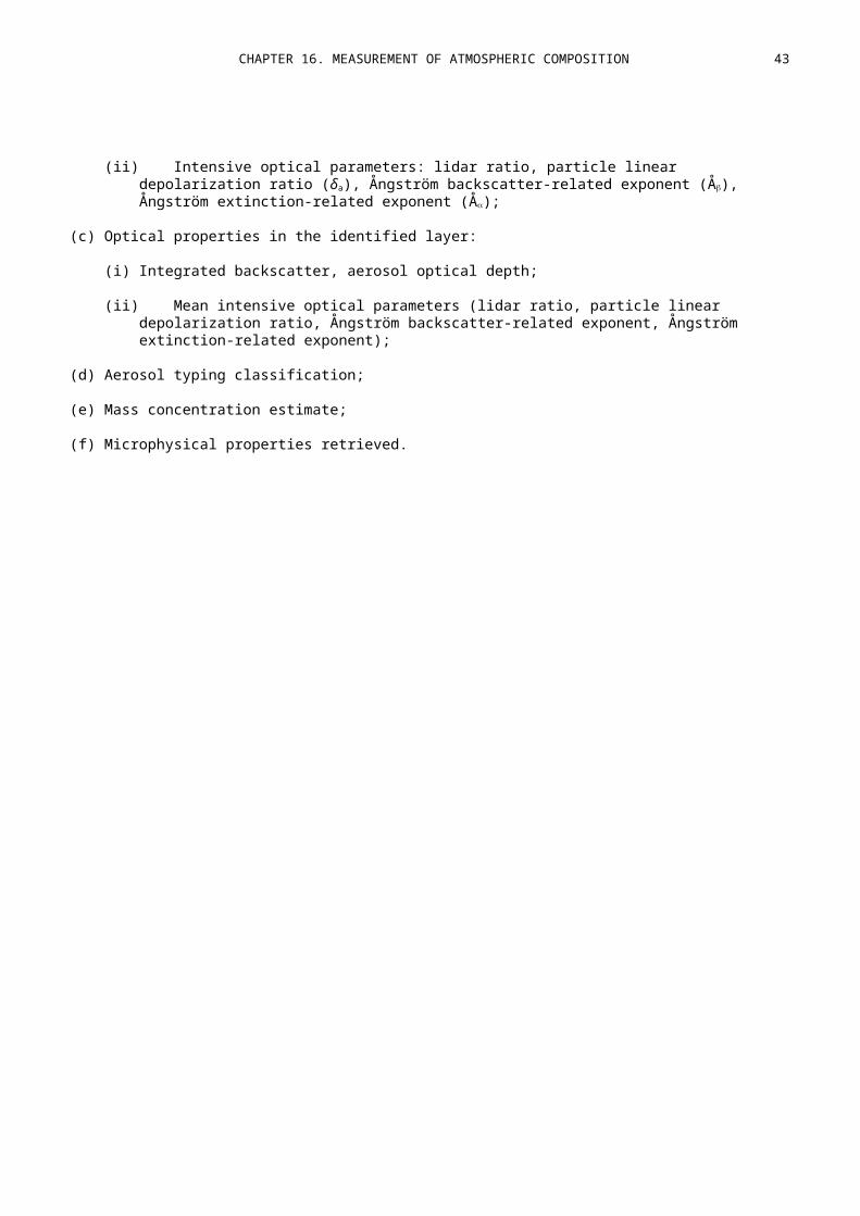
CHAPTER 16. MEASUREMENT OF ATMOSPHERIC COMPOSITION 43
Mateer, C.L. and J.J. DeLuisi, 1992: A new Umkehr inversion algorithm. Journal of Atmospheric and Terrestrial Physics, 54(5):537–556.
Mateer, C.L. and H.U. Dütsch, 1964: Uniform Evaluation of Umkehr Observations from the World Ozone Net-work, Part I – Proposed Standard Evaluation Technique, NCAR, Boulder, Colorado.
National Institute for Occupational Safety and Health, 2014: Elemental Carbon (Diesel Particulate): Method 5040 (available from http://www.cdc.gov/niosh/docs/2003-154/method-6000.html).
Petropavlovskikh, I., P.K. Bhartia and J. DeLuisi, 2005: New Umkehr ozone profile retrieval algorithm optimized for climatological studies. Geophysical Research Letters, 32(L16808).
Petzold, A., J.A. Ogren, M. Fiebig, P. Laj, S.-M. Li, U. Baltensperger, T. Holzer-Popp, S. Kinne, G. Pappalardo, N. Sugimoto, C. Wehrli, A. Wiedensohler and X.-Y. Zhang, 2013: Recommendations for reporting "black carbon" measurements. Atmospheric Chemistry and Physics, 13:8365–8379.
Ramanathan, K.R. and J.V. Dave, 1957: The calculation of the vertical distribution of ozone by the Götz Umkehr Effect (method B). Annals of the International Geophysical Year, V(1):23–45.
Schmid, H., L. Laskus, H.J. Abraham, U. Baltensperger, V. Lavanchy, M. Bizjak, P. Burba, H. Cachier, D. Crow, J. Chow, T. Gnauk, A. Even, H.M. ten Brink, K.P. Giesen, R. Hitzenberger, C. Hueglin, W. Maenhaut, C. Pio, A. Carvalho, J.-P. Putaud, D. Toom-Sauntry and H. Puxbaum, 2001: Results of the "carbon con-ference" international aerosol carbon round robin test stage I. Atmospheric Environment, 35(12):2111–2121.
Sofieva, V.F., N. Rahpoe, J. Tamminen, E. Kyrölä, N. Kalakoski, M. Weber, A. Laeng, T. von Clarmann, G. Stiller, S. Lossow, D. Degenstein, A. Bourassa, C. Adams, C. Roth, N. Lloyd, P. Bernath, R.J. Hargreaves, J. Urban, D. Murtagh, A. Hauchecorne, M. van Roozendael, N. Kalb and C. Zehner, 2013: Harmonized dataset of ozone profiles from satellite limb and occultation measurements. Earth System Science Data Discussions, 6:189–222.
Tegtmeier, S., M.I. Hegglin, J. Anderson, A. Bourassa, S. Brohede, D. Degenstein, L. Froidevaux, R. Fuller, B. Funke, J. Gille, A. Jones, Y. Kasai, K. Krüger, E. Kyrölä, G. Lingenfelser, J. Lumpe, B. Nardi, J. Neu, D. Pendlebury, E. Remsberg, A. Rozanov, L. Smith, M. Toohey, J. Urban, T. von Clarmann, K.A. Walker, and R. Wang, 2013: SPARC Data Initiative: A comparison of ozone climatologies from international limb satellite sounders. Journal of Geophysical Research, 118:12229–12247.
Tuzson, B., K. Zeyer, M. Steinbacher, J.B. McManus, D.D. Nelson, M.S. Zahniser and L. Emmenegger, 2013: Se-lective measurements of NO, NO2 and NOy in the free troposphere using quantum cascade laser spectroscopy. Atmospheric Measurement Techniques, 6:927–936.
Van der A, R. J., M.A.F. Allaart and H.J. Eskes, 2010: Multi sensor reanalysis of total ozone. Atmospheric Chem-istry and Physics, 10:11277–11294.
Warneke, C., P. Veres, J.S. Holloway, J. Stutz, C. Tsai, S. Alvarez, B. Rappenglueck, F.C. Fehsenfeld, M. Graus, J.B. Gilman and J.A. de Gouw, 2011: Airborne formaldehyde measurements using PTR-MS: calibra-tion, humidity dependence, inter-comparison and initial results. Atmospheric Measurement Tech-niques, 4:2345–2358.
Watson, J.G., J.C. Chow, L.-W. A. Chen and N.H. Frank, 2009: Methods to assess carbonaceous aerosol sampling artifacts for IMPROVE and other long-term networks. Journal of the Air and Waste Man-agement Association, 59(8):898–911.
Wisthaler, A., E.C. Apel, J. Bossmeyer, A. Hansel, W. Junkermann, R. Koppmann, R. Meier, K. Müller, S.J. So-lomon, R. Steinbrecher, R. Tillmann and T. Brauers, 2008: Technical note: Intercomparison of form-aldehyde measurements at the atmosphere simulation chamber SAPHIR. Atmospheric Chemistry and Physics, 8:2189–2200.
World Meteorological Organization, 2001: Global Atmosphere Watch Measurements Guide. Global Atmosphere Watch Report No. 143 (WMO/TD-No. 1073). Geneva.
———, 2003a: Quality Assurance in Monitoring Solar Ultraviolet Radiation: the State of the Art (A.R. Webb). Global Atmosphere Watch Report No. 146 (WMO/TD-No. 1180). Geneva.
———, 2003b: WMO/GAW Aerosol Measurement Procedures: Guidelines and Recommendations. Global Atmo-sphere Watch Report No. 153 (WMO/TD-No. 1178). Geneva.
———, 2004a: 1st International Expert Meeting on Sources and Measurements of Natural Radionuclides Ap-plied to Climate and Air Quality Studies (Gif sur Yvette, France, 3–5 June 2003). Global Atmosphere Watch Report No. 155 (WMO/TD-No. 1201). Geneva.
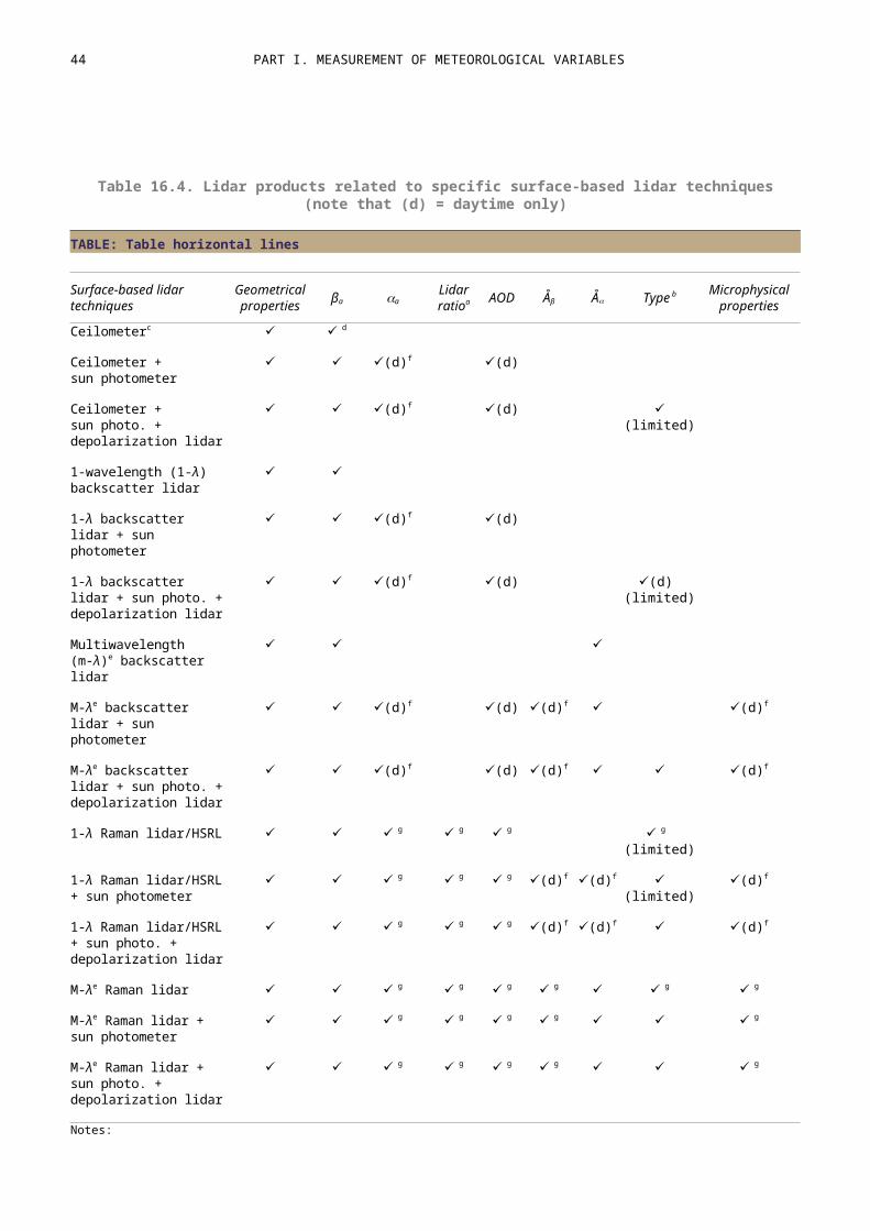
44 PART I. MEASUREMENT OF METEOROLOGICAL VARIABLES
———, 2004b: Manual for the GAW Precipitation Chemistry Programme (Guidelines, Data Quality Objectives and Standard Operating Procedures) (M.A. Allan, ed.). Global Atmosphere Watch Report No. 160 (WMO/TD-No. 1251). Geneva.
———, 2005: WMO/GAW Experts Workshop on a Global Surface-based Network for Long Term Observations of Column Aerosol Optical Properties (U. Baltensperger, L. Barrie and C. Wehrli, eds.) (Davos, Switzer-land, 8–10 March 2004). Global Atmosphere Watch Report No. 162 (WMO/TD-No. 1287). Geneva.
———, 2006: 13th WMO/IAEA Meeting of Experts on Carbon Dioxide Concentration and Related Tracers Meas-urement Techniques (J.B. Miller, ed.) (Boulder, Colorado, USA, 19–22 September 2005). Global At-mosphere Watch Report No. 168 (WMO/TD-No. 1359). Geneva.
———, 2007a: A WMO/GAW Expert Workshop on Global Long-Term Measurements of Volatile Organic Com-pounds (VOCs) (Geneva, Switzerland, 30 January to 1 February 2006). Global Atmosphere Watch Report No. 171 (WMO/TD-No. 1373). Geneva.
———, 2007b: WMO Global Atmosphere Watch (GAW) Strategic Plan: 2008–2015. Global Atmosphere Watch Report No. 172 (WMO/TD-No. 1384). Geneva.
———, 2008a: The Tenth Biennial WMO Consultation on Brewer Ozone and UV Spectrophotometer Operation, Calibration and Data Reporting (C.T. McElroy and E.W. Hare, eds.) (Northwich, United Kingdom, 4–8 June 2007). Global Atmosphere Watch Report No. 176 (WMO/TD-No. 1420). Geneva.
———, 2008b: Plan for the Implementation of the GAW Aerosol Lidar Observation Network GALION (J. Bösen-berg and R. Hoff) (Hamburg, Germany, 27–29 March 2007). Global Atmosphere Watch Report No. 178 (WMO/TD-No. 1443). Geneva.
———, 2008c: Operations Handbook – Ozone Observations with a Dobson Spectrophotometer (R.D. Evans, rev.). Global Atmosphere Watch Report No. 183 (WMO/TD-No. 1469). Geneva.
———, 2009a: Guidelines for the Measurement of Methane and Nitrous Oxide and their Quality Assurance. Global Atmosphere Watch Report No. 185 (WMO/TD-No. 1478). Geneva.
———, 2010: Guidelines for the Measurement of Atmospheric Carbon Monoxide. Global Atmosphere Watch Report No. 192 (WMO/TD-No. 1551). Geneva.
———, 2011a: WMO/GAW Expert Workshop on Global Long-term Measurements of Nitrogen Oxides and Re-commendations for GAW Nitrogen Oxides Network (S. Penkett, S. Gilge, C. Plass-Duelmer and I. Galbally) (Hohenpeissenberg, Germany, 8–9 October 2009). Global Atmosphere Watch Report No. 195 (WMO/TD-No. 1570). Geneva.
———, 2011b: Addendum for the Period 2012–2015 to the WMO Global Atmosphere Watch (GAW) Strategic Plan 2008–2015 (J. Klausen, ed.). Global Atmosphere Watch Report No. 197. Geneva.
———, 2011c: WMO/GAW Standard Operating Procedures for In-situ Measurements of Aerosol Mass Concen-tration, Light Scattering and Light Absorption (J.A. Ogren, ed.). Global Atmosphere Watch Report No. 200. Geneva.
———, 2012a: Standard Operating Procedures (SOPs) for Air Sampling in Stainless Steel Canisters for Non-Methane Hydrocarbons Analysis (R. Steinbrecher and E. Weiß). Global Atmosphere Watch Report No. 204. Geneva.
———, 2012b: 16th WMO/IAEA Meeting on Carbon Dioxide, Other Greenhouse Gases and Related Measure-ment Techniques (GGMT-2011) (G. Brailsford, ed.) (Wellington, New Zealand, 25–28 October 2011). Global Atmosphere Watch Report No. 206. Geneva.
———, 2013: Guidelines for Continuous Measurements of Ozone in the Troposphere (I.E. Galbally and M.G. Schultz). Global Atmosphere Watch Report No. 209 (WMO-No. 1110). Geneva.
———, 2014a: Quality Assurance and Quality Control for Ozonesonde Measurements in GAW (H.G.J. Smit and ASOPOS Panel). Global Atmosphere Watch Report No. 201. Geneva.
———, 2014b: Rationalizing Nomenclature for UV Doses and Effects on Humans (CIE209:2014/GAW Report No. 211) (ISBN: 978-3-902842-35-0)
———, 2014c: Standard Operating Procedures (SOPs) for Spectral Instruments Measuring Spectral Solar Ultra-violet Irradiance, Global Atmosphere Watch Report No. 212. Geneva.

CHAPTER 16. MEASUREMENT OF ATMOSPHERIC COMPOSITION 45
———, 2015a: Seventh Intercomparison Campaign of the Regional Brewer Calibration Center Europe (RBCC-E), (Lichtklimatisches Observatorium, Arosa, Switzerland, 16-27 July 2012), Global Atmosphere Watch Report No. 216. Geneva.
———, 2015b: Report of the Second Session of the CAS Environmental Pollution and Atmospheric Chemistry Scientific Steering Committee (EPAC SSC), (Geneva, Switzerland, 18-20 February 2015). Global Atmosphere Watch Report No. 220. Geneva.
———, 2015c: Absorption Cross-Sections of Ozone (ACSO) Status Report as of December 2015, Global Atmo-sphere Watch Report No. 218. Geneva.
———, 2015d: Analytical Methods for Atmospheric SF6 Using Gas Chromatography with micro Electron Cap-ture Detector (GC-μECD), Global Atmosphere Watch Report No. 222 (KMA Technical Note CCMD 2015-3). Geneva.
———, 2015e: Eighth Intercomparison Campaign of the Regional Brewer Calibration Center for Europe (RBCC-E), (El Arenosillo Sounding Station, Heulva, Spain, 10-20 June 2013), Global Atmosphere Watch Report No. 223. Geneva.
———, 2015f: Ninth Intercomparison Campaign of the Regional Brewer Calibration Center for Europe (RBCC-E), (Lichtklimatisches Observatorium, Arosa, Switzerland, 14-26 July 2014). Global Atmosphere Watch Report No. 224. Geneva.
———, 2016a: WMO/UNEP Dobson Data Quality Workshop, (Hradec Kralove, Czech Republic, 14-18 February 2011), Global Atmosphere Watch Report No. 225. Geneva.
———, 2016b: WMO/GAW Aerosol Measurement Procedures, Guidelines and Recommendations, 2nd Edition, Global Atmosphere Watch Report No. 227 (WMO-No. 1177). Geneva.
———, 2016c: 18th WMO/IAEA Meeting on Carbon Dioxide, Other Greenhouse Gases and Related Tracers Measurement Techniques (GGMT-2015), (La Jolla, CA, USA, 13-17 September 2015), Global Atmo-sphere Watch Report No. 229. Geneva.
———, 2017a: WMO Global Atmosphere Watch (GAW) Implementation Plan: 2016-2023. Global Atmosphere Watch Report No. 228. Geneva.
———, 2017b: Report of the WMO/GAW Expert Meeting on Nitrogen Oxides and International Workshop on the Nitrogen Cycle, (York, United Kingdom, 12 - 14 April 2016), Global Atmosphere Watch Report No. 232. Geneva.
![Dessler Fhrm3 Inppt01--Gaw[Rev] Sd](https://static.fdocuments.us/doc/165x107/577cc38a1a28aba711965140/dessler-fhrm3-inppt01-gawrev-sd.jpg)