Measurement Error and Linear Regression of …astrostatistics.psu.edu/su07/kelley_measerr07.pdf ·...

Measurement Error andLinear Regression ofAstronomical Data

Brandon KellyPenn State Summer School in

Astrostatistics, June 2007

Classical Regression Model• Collect n data points, denote ith pair as (ηi, ξi),

where η is the dependent variable (or‘response’), and ξ is the independent variable(or ‘predictor’, ‘covariate’)

• Assume usual additive error model:

!

"i=# + $%

i+ &

i

E(&i) = 0

Var(&i) = E(&

i

2) =' 2

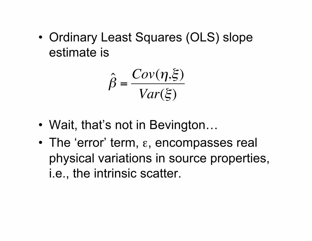
• Ordinary Least Squares (OLS) slopeestimate is

• Wait, that’s not in Bevington…• The ‘error’ term, ε, encompasses real

physical variations in source properties,i.e., the intrinsic scatter.!

ˆ " =Cov(#,$)

Var($)

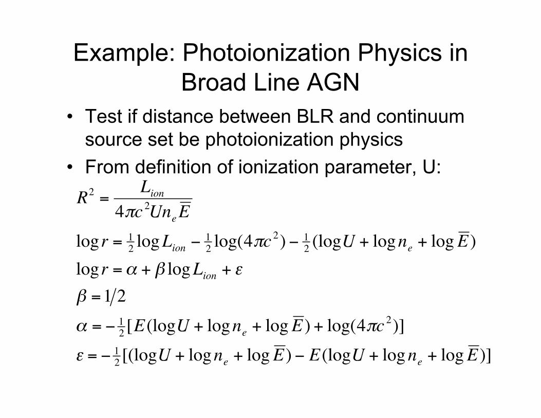
Example: Photoionization Physics inBroad Line AGN

• Test if distance between BLR and continuumsource set be photoionization physics

• From definition of ionization parameter, U:

!

R2

=L

ion

4"c2Un

eE

log r = 12logL

ion# 12log(4"c

2) # 12(logU + logn

e+ logE )

log r =$ + % logLion

+ &

% =1 2

$ = # 12[E(logU + logn

e+ logE ) + log(4"c

2)]

& = # 12[(logU + logn

e+ logE ) # E(logU + logn

e+ logE )]

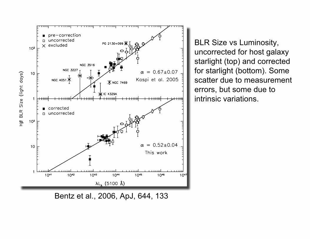
Bentz et al., 2006, ApJ, 644, 133

BLR Size vs Luminosity, uncorrected for host galaxy starlight (top) and corrected for starlight (bottom). Somescatter due to measurementerrors, but some due to intrinsic variations.

Measurement Errors• Don’t observe (η,ξ), but measured

values (y,x) instead.• Measurement errors add an additional

level to the statistical model:

!

"i =# + $% i + &i, E(&i) = 0, E(&i2) =' 2

xi = % i + &x,i, E(&x,i) = 0, E(&x,i2) =' x,i

2

yi ="i + &y,i, E(&y,i) = 0, E(&y,i2) =' y,i

2

E(&x,i&y,i) =' xy,i

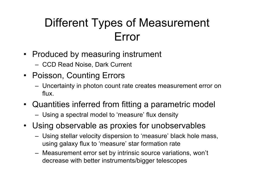
Different Types of MeasurementError

• Produced by measuring instrument– CCD Read Noise, Dark Current

• Poisson, Counting Errors– Uncertainty in photon count rate creates measurement error on

flux.

• Quantities inferred from fitting a parametric model– Using a spectral model to ‘measure’ flux density

• Using observable as proxies for unobservables– Using stellar velocity dispersion to ‘measure’ black hole mass,

using galaxy flux to ‘measure’ star formation rate– Measurement error set by intrinsic source variations, won’t

decrease with better instruments/bigger telescopes

Measurement errors alter the moments of thejoint distribution of the response and covariate,bias the correlation coefficient and slopeestimate

• If measurement errors are uncorrelated,regression slope unaffected by measurementerror in the response

• If errors uncorrelated, regression slope andcorrelation biased toward zero (attenuated).

!

ˆ b =Cov(x, y)

Var(x)=

Cov(",#) +$ xy

Var(") +$ x

2

ˆ r =Cov(x, y)

[Var(x)Var(y)]1/ 2

=Cov(",#) +$ xy

[Var(") +$ x

2]1/ 2

[Var(#) +$ y

2]1/ 2

Degree of Bias Depends onMagnitude of Measurement Error

• Define ratios ofmeasurement errorvariance to observedvariance:

• Bias can then beexpressed as:

!

RX =" x

2

Var(x), RY =

" y

2

Var(y),

RXY =" xy

Cov(x,y)

!

ˆ b

ˆ " =

1# RX

1# RXY

,ˆ r

ˆ $ =

(1# RX

)1/ 2

(1# RY)1/ 2

1# RXY

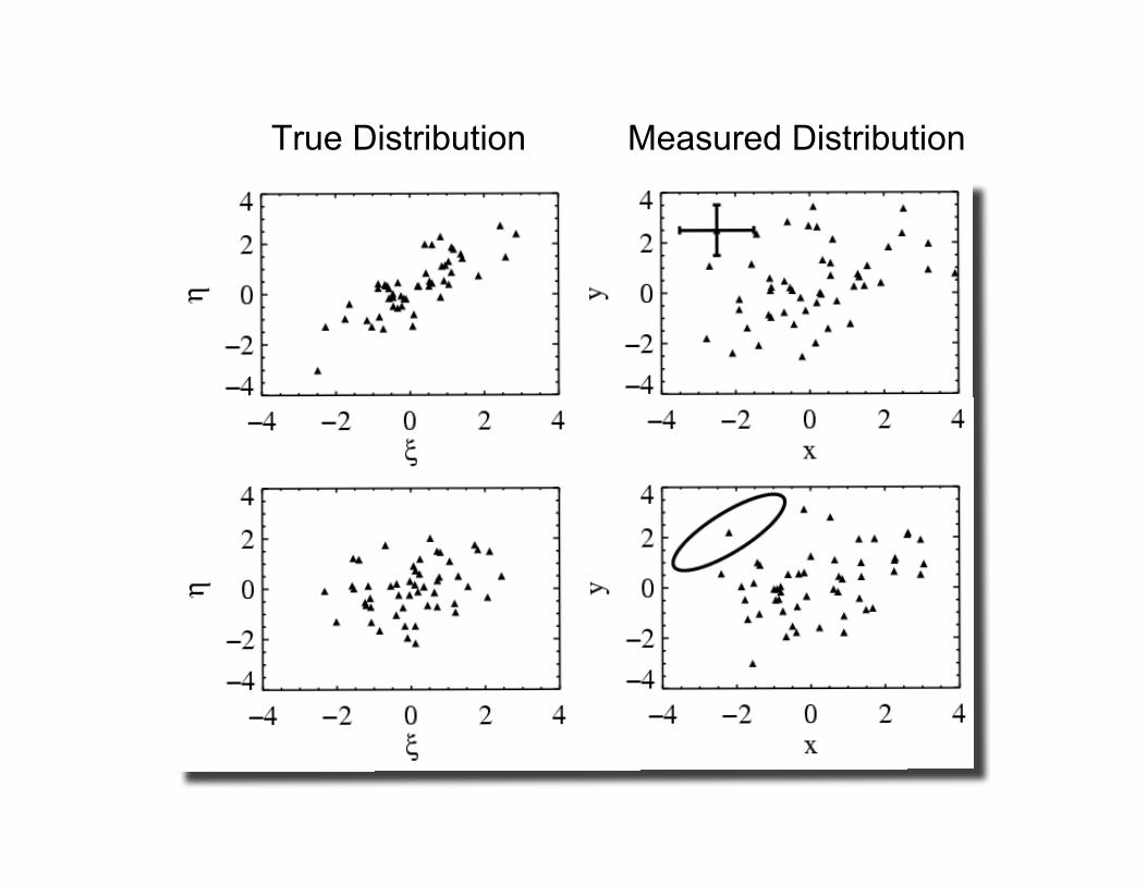
True Distribution Measured Distribution

BCES Estimator• BCES Approach (Akritas & Bershady, ApJ, 1996,

470, 706; see also Fuller 1987, Measurement ErrorModels) is to ‘debias’ the moments:

• Also give estimator for bisector and orthogonalregression slopes

• Asymptotically normal, variance in coefficients can beestimated from the data

• Variance of measurement error can depend onmeasured value

!

ˆ " BCES =Cov(x, y) #$ xy

Var(x) #$ x2

, ˆ % BCES = y # ˆ " BCES x

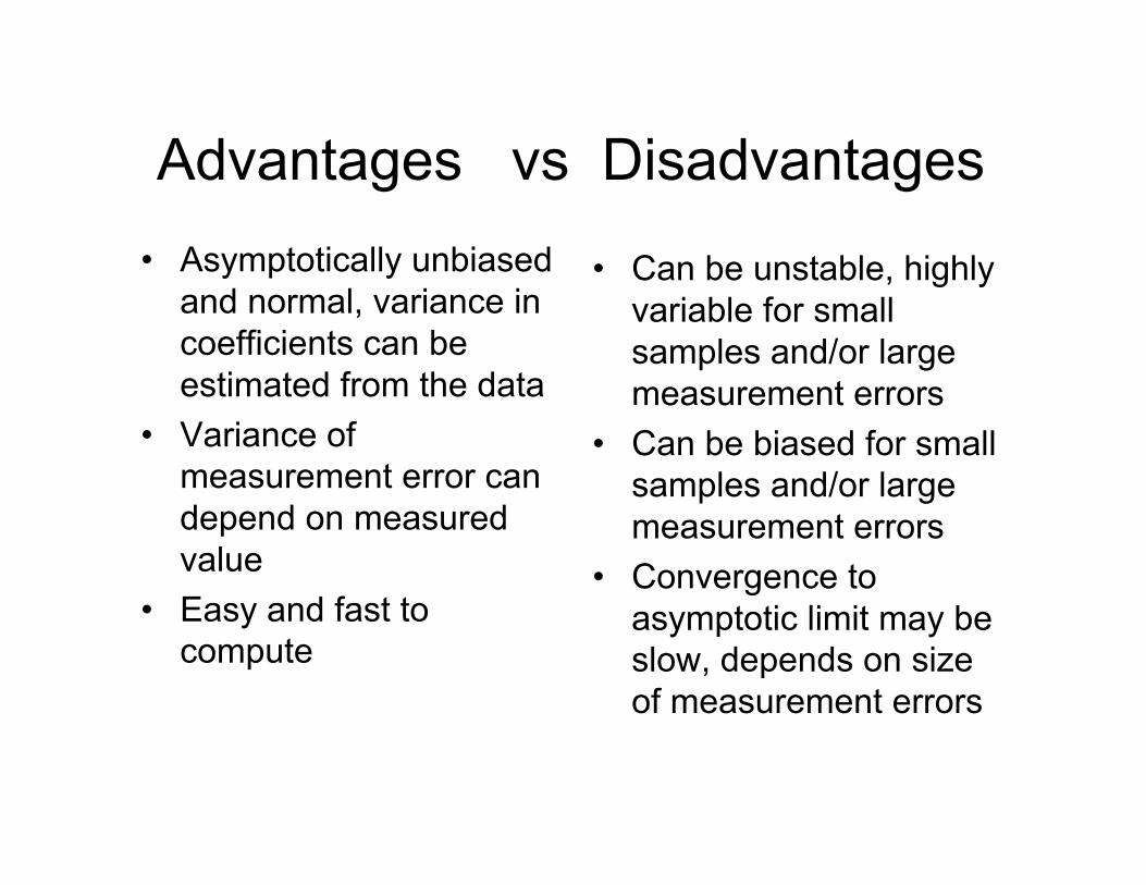
Advantages vs Disadvantages• Asymptotically unbiased

and normal, variance incoefficients can beestimated from the data

• Variance ofmeasurement error candepend on measuredvalue

• Easy and fast tocompute

• Can be unstable, highlyvariable for smallsamples and/or largemeasurement errors

• Can be biased for smallsamples and/or largemeasurement errors

• Convergence toasymptotic limit may beslow, depends on sizeof measurement errors

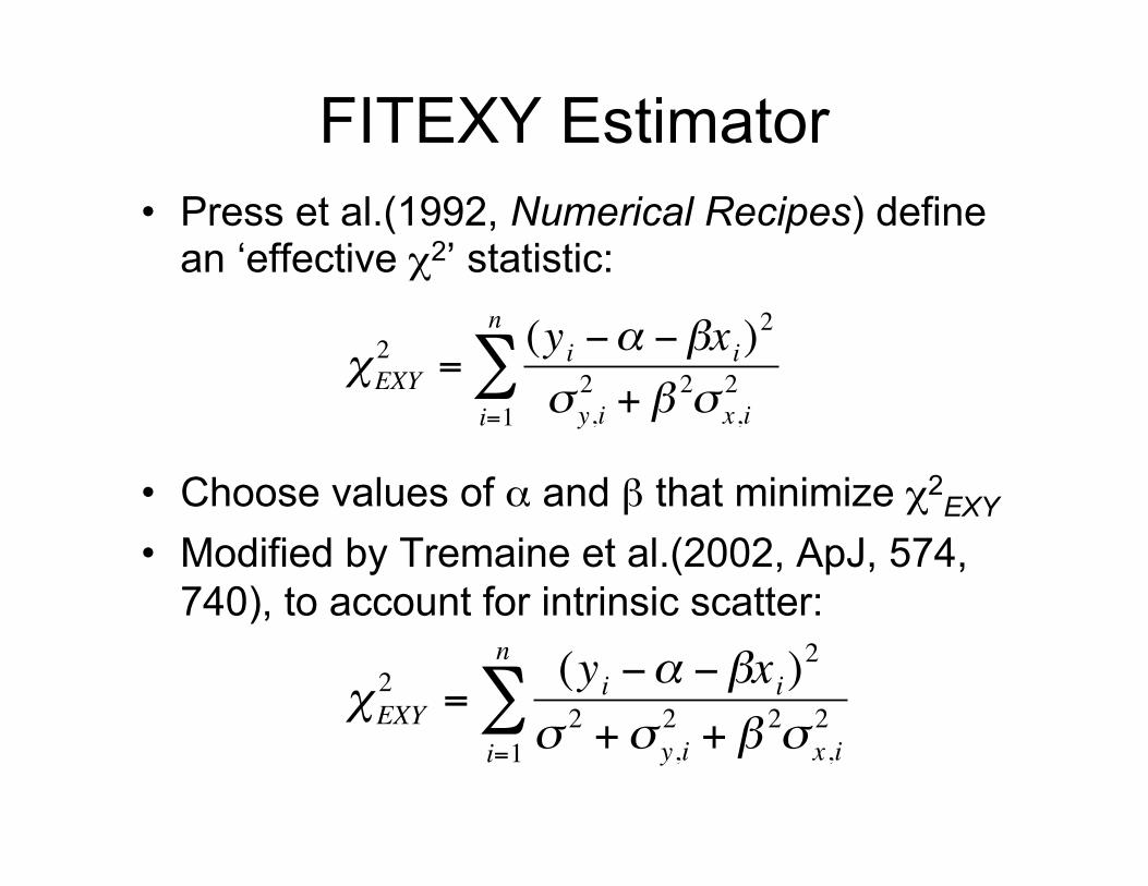
FITEXY Estimator• Press et al.(1992, Numerical Recipes) define

an ‘effective χ2’ statistic:

• Choose values of α and β that minimize χ2EXY

• Modified by Tremaine et al.(2002, ApJ, 574,740), to account for intrinsic scatter:!

"EXY

2=

(yi #$ #%xi)2

& y,i

2+ % 2& x,i

2

i=1

n

'

!

"EXY

2=

(yi #$ #%xi)2

& 2+& y,i

2+ % 2& x,i

2

i=1

n

'

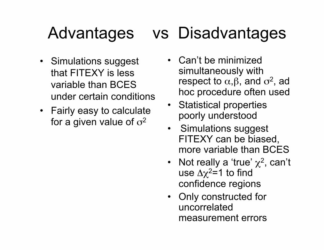
Advantages vs Disadvantages• Simulations suggest

that FITEXY is lessvariable than BCESunder certain conditions

• Fairly easy to calculatefor a given value of σ2

• Can’t be minimizedsimultaneously withrespect to α,β, and σ2, adhoc procedure often used

• Statistical propertiespoorly understood

• Simulations suggestFITEXY can be biased,more variable than BCES

• Not really a ‘true’ χ2, can’tuse Δχ2=1 to findconfidence regions

• Only constructed foruncorrelatedmeasurement errors

Structural Approach• Regard ξ and η as missing data, random

variables with some assumed probabilitydistribution

• Derive a complete data likelihood:

• Integrate over the missing data, ξ and η, toobtain the observed (measured) datalikelihood function!

p(x,y,",# |$,%) = p(x,y |",#)p(# |",$)p(" |%)

!

p(x,y |",#) = p(x,y,$,% |",#)d$ d%&&

Mixture of Normals Model• Model the distribution of ξ as a mixture of K

Gaussians, assume Gaussian intrinsic scatterand Gaussian measurement errors of knownvariance

• The model is hierarchically expressed as:

!

" i |# ,µ,$2~ # kN(µk,$ k

2)

k=1

K

%

&i |" i,',(,)2~ N(' + (" i,)

2)

yi,xi |&i," i ~ N([&i," i],*i)

+ = (# ,µ,$ 2), , = (',(,) 2), *i =

) y,i

2 ) xy,i

) xy,i ) x,i

2

-

. /

0

1 2

References: Kelly (2007, ApJ in press, arXiv:705.2774), Carroll et al.(1999, Biometrics, 55, 44)

Integrate complete data likelihood toobtain observed data likelihood:

!

p(x,y |",#) = p(xi,yi |$ i,%i)p(%i |$ i,")p($ i |#)&& d$ i d%i

i=1

n

'

=( k

2( Vk,i

1/ 2exp ) 1

2(z i )* k )

TVk,i

)1(z i )* k ){ }k=1

K

+i=1

n

'

z i = yi xi( )T

* k = , + -µk µk( )T

Vk,i =- 2. k

2 +/ 2 +/ y,i

2 -. k2 +/ xy,i

-. k2 +/ xy,i . k

2 +/ x,i

2

0

1 2

3

4 5

Can be used to calculate a maximum-likelihoodestimate (MLE), perform Bayesian inference. See Kelly(2007) for generalization to multiple covariates.

What if we assume that ξ has auniform distribution?

• The likelihood for uniform p(ξ) can beobtained in the limit τ ∞:

• Argument of exponential is χ2EXY statistic!

• But minimizing χ2EXY is not the same as

maximizing the likelihood…• For homoskedastic measurement errors,

maximizing this likelihood leads to theordinary least-squares estimate, so stillbiased.

!

p(x,y |")# $ 2 +$ y,i

2 + % 2$ x,i

2( )&1

2 exp &1

2

(yi &' &%xi)2

$ 2 +$ y,i

2 + % 2$ x,i

2

( ) *

+ , - i=1

n

.

Advantages vs Disadvantages• Simulations suggest MLE for

normal mixture approximatelyunbiased, even for smallsamples and largemeasurement error

• Lower variance than BCES andFITEXY

• MLE for σ2 rarely, if ever, equalto zero

• Bayesian inference can beperformed, valid for any samplesize

• Can be extended to handlenon-detections, truncation,multiple covariates

• Simultaneously estimatesdistribution of covariates, maybe useful for some studies

• Computationally intensive,more complicated thanBCES and FITEXY

• Assumes measurement errorvariance known, does notdepend on measurement

• Needs a parametric form forthe intrinsic distribution ofcovariates (but mixturemodel flexible and fairlyrobust).

Simulation Study: Slope

Dashed lines mark the median value of the estimator, solid linesmark the true value of the slope. Each simulated data set had 50data points, and y-measurement errors of σy ~ σ.

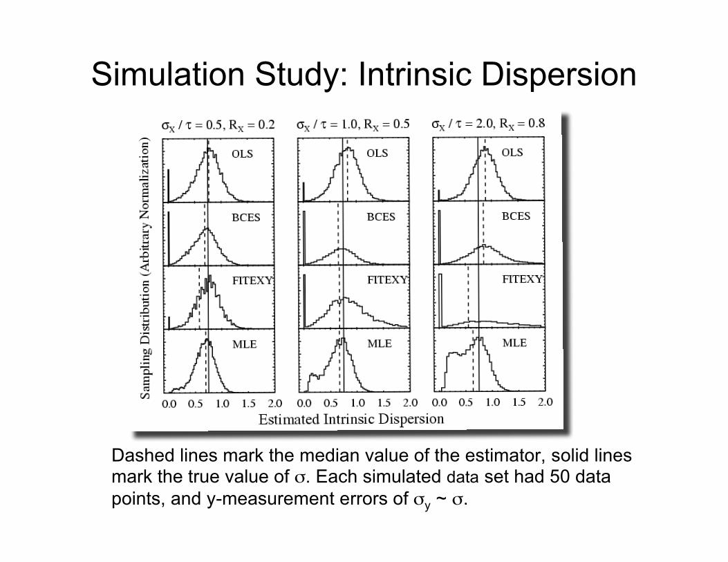
Simulation Study: Intrinsic Dispersion

Dashed lines mark the median value of the estimator, solid linesmark the true value of σ. Each simulated data set had 50 datapoints, and y-measurement errors of σy ~ σ.

Effects of Sample Selection• Suppose we select a sample of n sources,

out of a total of N possible sources• Introduce indicator variable, I, denoting

whether a source is included. Ii = 1 if the ithsource is included, otherwise Ii = 0.

• Selection function for ith source is p(Ii=1|yi,xi)• Selection function gives the probability that

the ith source is included in the sample, giventhe values of xi and yi.

See Little & Rubin (2002, Statistical Analysis with Missing Data) orGelman et al.(2004, Bayesian Data Analysis) for further reading.

• Complete data likelihood is

• Here, Aobs denotes the set of n included sources, andAmis denotes the set of N-n sources not included

• Binomial coefficient gives number of possible ways toselect a subset of n sources from a sample of Nsources

• Integrating over the missing data, the observed datalikelihood now becomes

!

p(x,y,",#,I |$,%,N)&N

n

'

( ) *

+ , p(xi,yi," i,#i,Ii |$,%)i-Aobs

. p(x j ,y j ," j ,# j ,I j |$,%)j-Amis

.

!

p(xobs,yobs,I |",#,N)$N

n

%

& ' (

) * p(xi,yi |",#)i+Aobs

,

- p(I j = 0 | x j ,y j )p(x j ,y j |",#).. dx j dy j

j+Amis

,

Selection only dependent oncovariates

• If the sample selection only depends on thecovariates, then p(I|x,y) = p(I|x).

• Observed data likelihood is then

• Therefore, if selection is only on thecovariates, then inference on the regressionparameters is unaffected by selection effects.!

p(xobs,yobs,I |",#,N)$N

n

%

& ' (

) * p(xi,yi |",#)i+Aobs

,

- p(I j = 0 | x j )p(y j | x j ,",#)p(x j |#).. dx j dy j

j+Amis

,

$N

n

%

& ' (

) * p(xi,yi | Ii =1,",#obs)i+Aobs

, p(x j | I j = 0,#mis)p(I j = 0 |#mis). dx j

j+Amis

,

Covariate Selection vsResponse Selection

Covariate Selection: Noeffect on distribution of y at agiven x

Response Selection:Changes distribution of y at agiven x

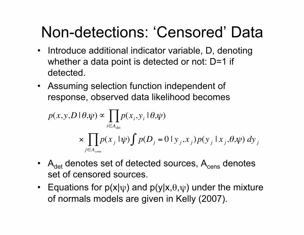
Non-detections: ‘Censored’ Data• Introduce additional indicator variable, D, denoting

whether a data point is detected or not: D=1 ifdetected.

• Assuming selection function independent ofresponse, observed data likelihood becomes

• Adet denotes set of detected sources, Acens denotesset of censored sources.

• Equations for p(x|ψ) and p(y|x,θ,ψ) under the mixtureof normals models are given in Kelly (2007).

!

p(x,y,D |",#)$ p(xi,yi |",#)i%Adet

&

' p(x j |#) p(Dj = 0 | y j ,x j )p(y j | x j ,",#) dy j(j%Acens

&

Bayesian Inference• Calculate posterior probability density

for mixture of normals structural model• Posterior valid for any sample size,

doesn’t rely on large sampleapproximations (e.g., asymptoticdistribution of MLE).

• Assume prior advocated by Carroll etal.(1999)

• Use markov chain monte carlo (MCMC)to obtain draws from posterior

Gibbs Sampler• Method for obtaining draws from posterior, easy

to program• Start with initial guesses for all unknowns• Proceed in three steps:

– Simulate new values of missing data, including non-detections, given the observed data and current values ofthe parameters

– Simulate new values of the parameters, given the currentvalues of the prior parameters and the missing data

– Simulate new values of the prior parameters, given thecurrent parameter values.

• Save random draws at each iterations, repeatuntil convergence.

• Treat values from latter part of Gibbs sampler asrandom draw form the posteriorDetails given in Kelly (2007). Computer routines available at IDL Astronomy User’s Library, http://idlastro.gsfc.nasa.gov/homepage.html

Example: Simulated Data Setwith Non-detections

Filled Squares: Detected data points

Hollow Squares: Undetected data points

Solid line is true regression line,Dashed-dotted is posterior Median, shaded region containsApproximately 95% of posteriorprobability

Posterior from MCMC for simulateddata with non-detections

Solid vertical line markstrue value. For comparison, a naïve MLE that ignores meas.error found

This is biased toward zero at a level of 3.5σ

!

"MLE

= 0.229 ± 0.077

Example: Dependence of Quasar X-raySpectral Slope on Eddington Ratio

Solid line is posterior median,Shaded region contains 95%Of posterior probability.

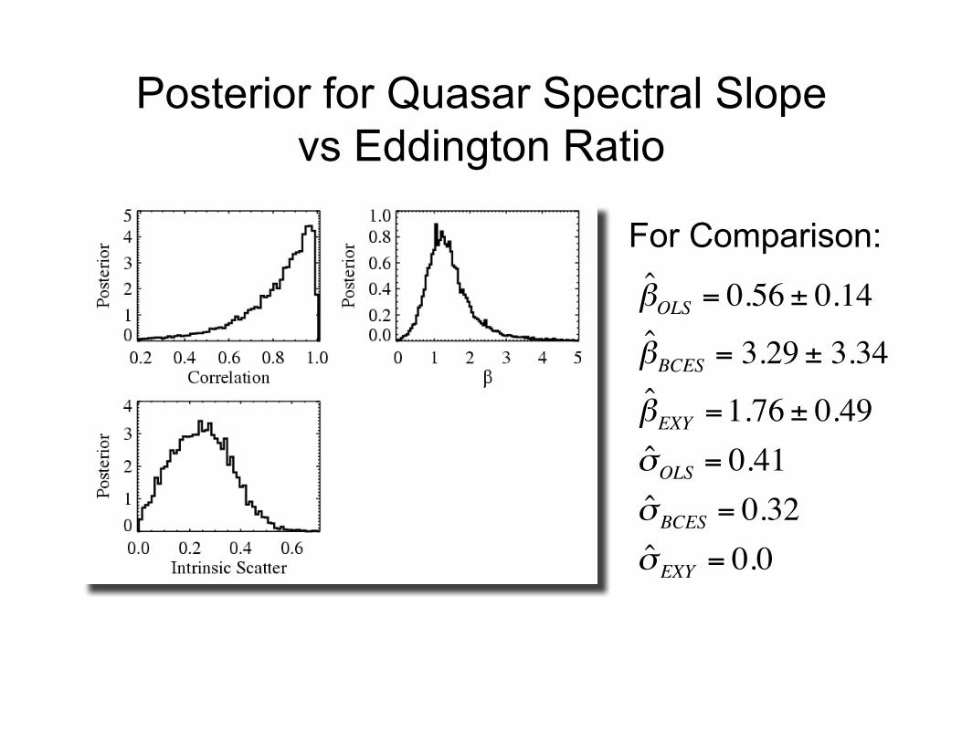
Posterior for Quasar Spectral Slopevs Eddington Ratio

For Comparison:

!

ˆ " OLS

= 0.56 ± 0.14

ˆ " BCES

= 3.29 ± 3.34

ˆ " EXY

=1.76 ± 0.49

ˆ # OLS

= 0.41

ˆ # BCES

= 0.32

ˆ # EXY

= 0.0

References• Akritas & Bershady, 1996, ApJ, 470, 706• Carroll, Roeder, & Wasserman, 1999, Biometrics, 55, 44• Carroll, Ruppert, & Stefanski, 1995, Measurement Error in

Nonlinear Models (London: Chapman & Hall)• Fuller, 1987, Measurement Error Models, (New York: John

Wiley & Sons)• Gelman et al., 2004, Bayesian Data Analysis, (2nd Edition; Boca

Raton: Chapman Hall/CRC)• Isobe, Feigelson, & Nelson, 1986, ApJ, 306, 490• Kelly, B.C, 2007, in press at ApJ (arXiv:705.2774)• Little & Rubin, 2002, Statistical Analysis with Missing Data (2nd

Edition; Hoboken: John Wiley & Sons)• Press et al., 1992, Numerical Recipes, (2nd Edition; Cambridge:

Cambridge Unv. Press)• Schafer, 1987, Biometrica, 74, 385• Schafer, 2001, Biometrics, 57, 53

Measurement Error and Linear Regression of …astrostatistics.psu.edu/su07/kelley_measerr07.pdf ·...

Documents

Transcript of Measurement Error and Linear Regression of …astrostatistics.psu.edu/su07/kelley_measerr07.pdf ·...