Measurement and simulation of surface

roughness noise using phased microphone

arrays ?

Y. Liu ∗, A.P. Dowling, H.-C. Shin

Department of Engineering, University of Cambridge, Trumpington Street,Cambridge CB2 1PZ, UK

Abstract

A turbulent boundary-layer flow over a rough wall generates a dipole sound fieldas the near-field hydrodynamic disturbances in the turbulent boundary-layer scatterinto radiated sound at small surface irregularities. In this paper, phased microphonearrays are applied to the measurement and simulation of surface roughness noise.The radiated sound from two rough plates and one smooth plate in an open jet ismeasured at three streamwise locations, and the beamforming source maps demon-strate the dipole directivity. Higher source strengths can be observed on the roughplates which also enhance the trailing-edge noise. A prediction scheme in previ-ous theoretical work is used to describe the strength of a distribution of incoherentdipoles and to simulate the sound detected by the microphone array. Source maps ofmeasurement and simulation exhibit satisfactory similarities in both source patternand source strength, which confirms the dipole nature and the predicted magnitudeof roughness noise. However, the simulations underestimate the streamwise gradi-ent of the source strengths and overestimate the source strengths at the highestfrequency.

Key words: surface roughness noise, aeroacoustic dipole, phased microphonearray, beamforming algorithm.

? Submitted to Journal of Sound and Vibration on 14 May 2007, accepted for pub-lication on 21 December 2007. Original version presented in the 13th AIAA/CEASAeroacoustics Conference, Rome, Italy, 21–23 May 2007.∗ Corresponding author. Tel.: +44 1223 766063; fax: +44 1223 330282.

Email address: yl275@cam.ac.uk (Y. Liu).

Preprint submitted to Elsevier 16 January 2008

Nomenclature

a monopole source strengthA area of the rough regionc speed of sound in free fieldd distance between microphones and their nearest neighbourD directivity functionf frequencyi

√−1

I1, I2 integrals with respect to the wavenumber vector κk acoustic wavenumberl distance between the two coherent monopoles of a dipoleM free stream Mach numbern number of frequency intervalsN average number of roughness bosses per unit areap acoustic frequency spectrumP power spectral density of pPR power spectral density of far-field radiated roughness noise spectrumPs smooth-wall wavenumber-frequency spectrumr propagation distanceR roughness heightReτ roughness Reynolds number, Reτ = Ruτ/νSh∗ Strouhal number, Sh∗ = ωδ∗/Uuτ friction velocityU free stream velocityUc eddy convection velocityx1 streamwise distance from the front edge of rough regionx,y,z Cartesian coordinatesδ boundary-layer thicknessδ∗ displacement boundary-layer thicknessδ(.) Dirac delta functionκ wavenumber vector, κ = (κ1, 0, κ3)Λ power spectral density of aµ roughness density factor, µ = 1/(1 + 1

4σ)

ν kinematic viscosityω radian frequencyΦ point pressure frequency spectrumρ0 mean fluid density in free fieldσ roughness densityτw mean wall shear stress, τw = ρ0u

2τ

θ, φ directivity angles¯ mean value

ensemble average+,− monopoles with opposite phase1, 2 dipoles DPL1 and DPL2

2

i, j general summation variabletot total powerDPL1 dipole in flow directionDPL2 dipole normal to flow directionCFT continuous Fourier transformDFT discrete Fourier transformFFT fast Fourier transformSPL sound pressure level

1 Introduction

The generation of sound by turbulent boundary-layer flow at low Mach num-ber over a rigid rough wall has been investigated analytically by Howe [1–4].In Howe’s diffraction theory, the rough surface was modelled by a randomdistribution of rigid, hemispherical bosses over a rigid plane. The near-fieldhydrodynamic disturbances in the turbulent boundary layer scatter into radi-ated sound due to the presence of small surface irregularities. The roughnesselements behave like point dipoles with the dipole strength due to scatteringof the near turbulent pressure fluctuations on an element, and thus surfaceroughness noise is likely to be dominant at low Mach number. Howe [1] alsospeculated that roughness noise would be a substantial fraction of the airframenoise of an airplane flying in the “clean” configuration in which the landinggears and high-lift devices are stowed.

In the theoretical model [1], the acoustic frequency spectrum PR(ω) of far-fieldradiated roughness noise was expressed as an infinite integral in terms of thesmooth-wall wavenumber-frequency spectrum Ps(κ, ω). Howe evaluated PR(ω)by means of a conventional asymptotic approximation [1,3] based on Ps(κ, ω)being sharply peaked in the vicinity of the convective ridge. He also proposedempirical models [3–5] for PR(ω) by curve-fitting available experimental dataof Hersh [6]. The empirical coefficients were partially estimated, but not all thecoefficient values could be determined due to the lack of directivity informationin Hersh’s data. Therefore, Howe’s empirical models are unable to predict theabsolute level of the rough-wall acoustic frequency spectrum PR(ω).

The theoretical model of Howe [1] was recently extended by Liu and Dowl-ing [7] to quantify numerically the far-field radiated roughness noise. They ap-proximated the rough-wall wavenumber-frequency spectrum by smooth-wallmodels [8–12] with increased friction velocity uτ and boundary-layer thicknessδ appropriate for a rough surface. The infinite integral in the determination ofPR(ω) was evaluated by direct numerical integration. Their prediction schemeis able to reproduce the spectral characteristics of Howe’s empirical models andHersh’s experimental data, and to predict appropriately the absolute level of

3

far-field radiated roughness noise.

Liu and Dowling [7] then applied the numerical method to the assessmentof the contribution of surface roughness to airframe noise, and estimatedthe roughness noise for a Boeing-757 sized aircraft wing during approach ortake-off with idealized levels of surface roughness. They found that in thehigh frequency region sound radiated from surface roughness may exceed thatfrom the trailing edge depending on the size of roughness elements, and thatthe trailing-edge noise is also enhanced by surface roughness to some extent.Therefore they suggested that the contribution of surface roughness to air-frame noise needs to be considered in the design of a low-noise airframe.

However, few experiments have been performed so far to investigate the noiseradiated from rough surfaces. Measurement of roughness noise is difficult as itcan be easily contaminated due to its very low spectral levels. Hersh [6] stud-ied the radiation of sound from sand-roughened pipes of various grit sizes. Heconcluded through measurements that the 6th power variation of the overallsound pressure level with flow velocity suggests a dipole source. However, thedata are insufficient for building an empirical model, as aforementioned, dueto the unknown effects of acoustic refraction by the free-jet shear layers down-stream of the nozzle exit. Liu and Dowling [7] measured the noise spectra oftwo rough plates with different roughness heights in an open jet. The mea-sured noise spectra were significantly contaminated by background noise, butthe roughness noise was detected in 1–2.5 kHz frequency range. The reason-able amount of agreement between measurement and prediction provided apreliminary validation of their numerical prediction scheme which was basedon Howe’s theoretical model [1].

In this paper, phased microphone arrays were applied to the experimentalstudy of surface roughness noise. The radiated sound from two rough platesand one smooth plate in an open jet was measured by both high- and low-frequency arrays. The source locations and source strengths of possible dipolesdue to roughness elements on a rigid plate were identified and discussed.Acoustic measurements were performed at three streamwise locations to ex-plore the directivity features of possible dipole sources. Theoretical predictionsfor the source distributions on the two rough plates were also obtained usingLiu and Dowling’s model [7].

However, the array measurements can be misinterpreted if applied directlyto determine the locations and relative strengths of these distributed dipoles,and this is due to the assumption of distributed incoherent monopoles in thestandard beamforming algorithm [13–15]. The technique developed by Jordanet al. [16] to account for the propagation characteristics of a single dipole isnot applicable because the roughness dipoles are distributed over such a largeregion that the directivity varies considerably. The array analysis source code

4

is inaccessible and so it was not possible to modify the algorithm to base thebeamforming on dipole sources.

Instead, we processed the theoretical cross-power spectral densities throughthe same beamforming algorithm as the experimental data and compared theresulting predicted and measured source maps. This is equivalent to compar-ing theory and experiment after applying a filter which suppresses much theextraneous noise in the experiments. A distribution of incoherent dipoles wassimulated over a rigid plate with the source strengths determined equivalentlyby the prediction scheme of Liu and Dowling [7]. Comparison of the results ofbeamforming between measurement and simulation provides indirect valida-tion of the predicted source type, magnitude and distribution.

2 Experimental setup

2.1 Test rough plate

The experiments were conducted in the open jet of a low-speed wind tunnelin the Whittle Laboratory of the Department of Engineering, Cambridge Uni-versity, as illustrated in Fig. 1. The wind tunnel has an inner cross section of0.586 × 0.350 m2 at the outlet and a velocity range of 0–31.0 m s−1. Plasticfoam lined in the inner walls and a splitter silencer was installed to reducethe wind noise and motor noise traveling inside the tunnel. A large flat platemade of aluminium alloy is placed nominally in the vertical meridian plane ofthe open jet. It is secured to a vertical frame of aluminium rods adjacent tothe tunnel outlet. Fig. 1(b) shows that the plate surface is partially roughenedin a rectangular region by a square distribution of hemispherical bosses. Thiswas achieved by machining a recess of 0.64 × 0.64 m2 into the plate surface.Four modeling panels of 0.32×0.32 m2 with rigid, hemispherical plastic beadsin parallel columns were flush mounted in the recess to form a rough region.Four smooth panels were also fabricated for the measurement of a smoothplate or a rough plate with a smaller rough region.

Three different surface conditions were examined:

(1) Rough1, R = 4 mm, σ = 0.50;(2) Rough2, R = 3 mm, σ = 0.44;(3) Smooth, R = 0 mm, σ = 0.0;

where R and σ are the roughness height and roughness density [1,7], respec-tively.

5

(a)

(b)

Fig. 1. Schematic of the experimental setup: (a) overview; (b) closeup.

The rough region is located at 0.34 m from the leading edge of the test plate,where the turbulent boundary layer is tripped, to ensure that the roughnesselements are contained entirely within the boundary layer[1,7] and to avoid theinterference of sound scattering at the leading edge. Acoustic measurementswere performed at free stream flow velocities, U = 15, 20, 25 and 30 m s−1.The roughness noise scales as U6 and so is more detectable at the highervelocity [7]. Therefore the experimental results discussed in §3 are for thevelocity U = 30 m s−1 when differences between the acoustic data of therough and smooth plates are most evident. As a precaution, all measurementswere made when the laboratory ventilation system was not in operation.

2.2 Phased microphone array

Phased microphone arrays were utilized to localize the possible dipole sourcesin the rough region. The advantage of phased microphone arrays lies in the

6

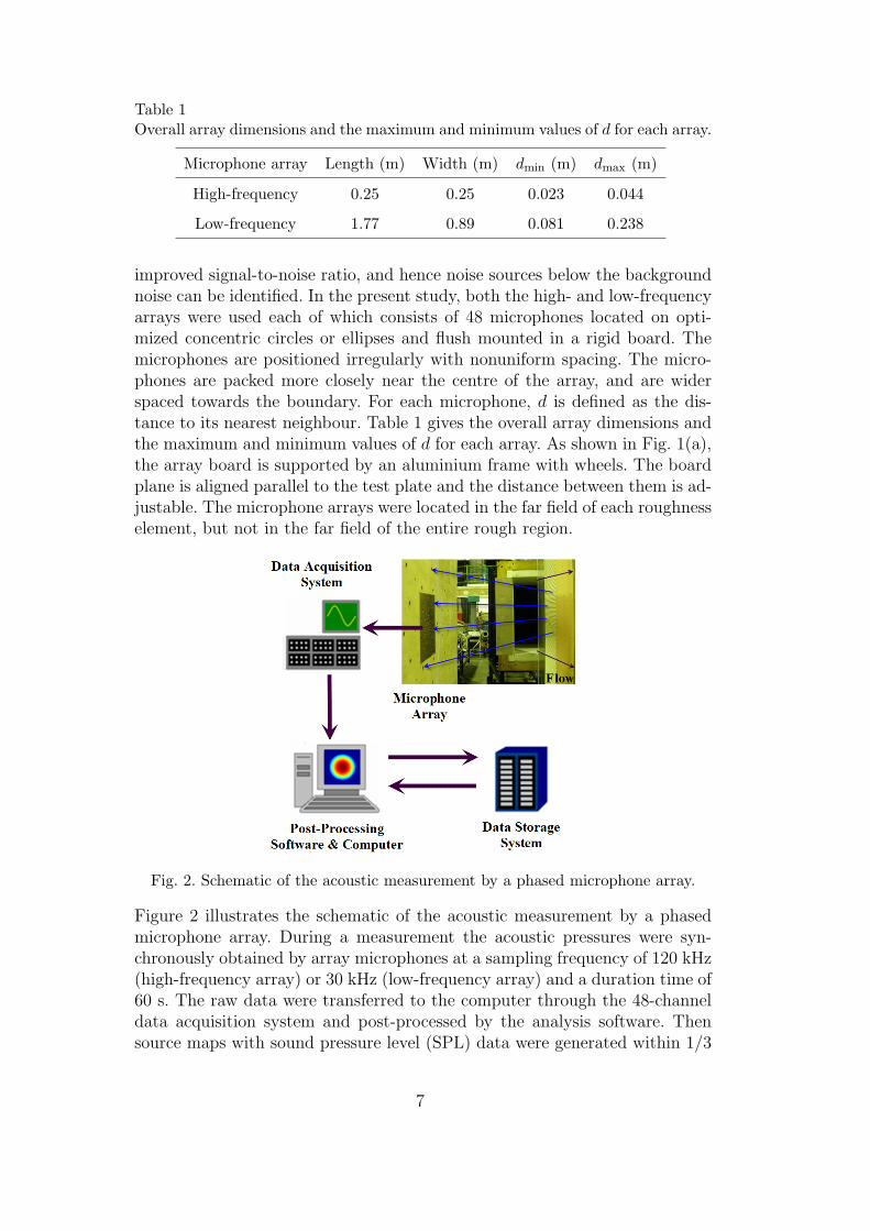
Table 1Overall array dimensions and the maximum and minimum values of d for each array.

Microphone array Length (m) Width (m) dmin (m) dmax (m)

High-frequency 0.25 0.25 0.023 0.044

Low-frequency 1.77 0.89 0.081 0.238

improved signal-to-noise ratio, and hence noise sources below the backgroundnoise can be identified. In the present study, both the high- and low-frequencyarrays were used each of which consists of 48 microphones located on opti-mized concentric circles or ellipses and flush mounted in a rigid board. Themicrophones are positioned irregularly with nonuniform spacing. The micro-phones are packed more closely near the centre of the array, and are widerspaced towards the boundary. For each microphone, d is defined as the dis-tance to its nearest neighbour. Table 1 gives the overall array dimensions andthe maximum and minimum values of d for each array. As shown in Fig. 1(a),the array board is supported by an aluminium frame with wheels. The boardplane is aligned parallel to the test plate and the distance between them is ad-justable. The microphone arrays were located in the far field of each roughnesselement, but not in the far field of the entire rough region.

Fig. 2. Schematic of the acoustic measurement by a phased microphone array.

Figure 2 illustrates the schematic of the acoustic measurement by a phasedmicrophone array. During a measurement the acoustic pressures were syn-chronously obtained by array microphones at a sampling frequency of 120 kHz(high-frequency array) or 30 kHz (low-frequency array) and a duration time of60 s. The raw data were transferred to the computer through the 48-channeldata acquisition system and post-processed by the analysis software. Thensource maps with sound pressure level (SPL) data were generated within 1/3

7

octave-band frequencies by beamforming 1 the post-processed data. The finaldata were sent to the 1.2 TB data storage system for future reference.

In the beamformer, the measured signals in the time domain are transformedto complex pressures in the frequency domain by the fast Fourier transform(FFT). The matrix of cross-power spectral densities between all microphonecombinations is formulated in the frequency domain. The open-jet tunnel hassome background noise and so we remove the diagonal elements of the matrix(i.e. the auto-power) and determine the monopole source strength at eachelement of the source grid that gives a best least-square fit to the measuredcross-powers. First, a scanning grid containing the test plate is defined. Themonopole source strength at each grid point is estimated by finding the valuewhich gives the best match between measured cross-powers and the field of amonopole located at that grid point. The beamformer used the true distancefrom each source element to each microphone.

Obviously, the advantage of an open jet is to eliminate the reverberation noiseof a closed-return wind tunnel. However, the uniform flow assumption of anal-ysis software is not valid in the case of out-of-flow measurements in the testsection of an open jet [17]. In this case, the effect of shear-layer refraction hasto be incorporated in the source description of beamforming analysis. In factfor the low-speed wind tunnel in use (M < 0.1), although the propagatingacoustic wave is somewhat refracted during transmission through the shearlayer, the amplitude of received acoustic pressure by array microphones is al-most unaltered, and hence the effect of shear-layer refraction on the predictedsource strengths is negligible [15]. However, even a minor error in the signalphase will be amplified into a considerable distortion of source locations. Inthis study, the Amiet correction [18] for an infinitely thin shear layer wasapplied in beamforming analysis for the shear-layer correction.

3 Results and discussion

3.1 Comparison of noise spectra

Firstly, the comparison of the noise spectra for the rough and smooth plates isshown in Fig. 3. These noise spectra were measured by a pair of microphonesat 0.3 m apart (r = 1.2 m, θ = π/4, φ = 0, see Fig. 8). The cross-spectra data

1 “Beamforming” refers to an algorithm for the phased microphone array which,for each position on the source scanning plane, determines the monopole sourcestrength at that location that best matches the data [13–15]. The beamformingcode is implemented in the frequency domain.

8

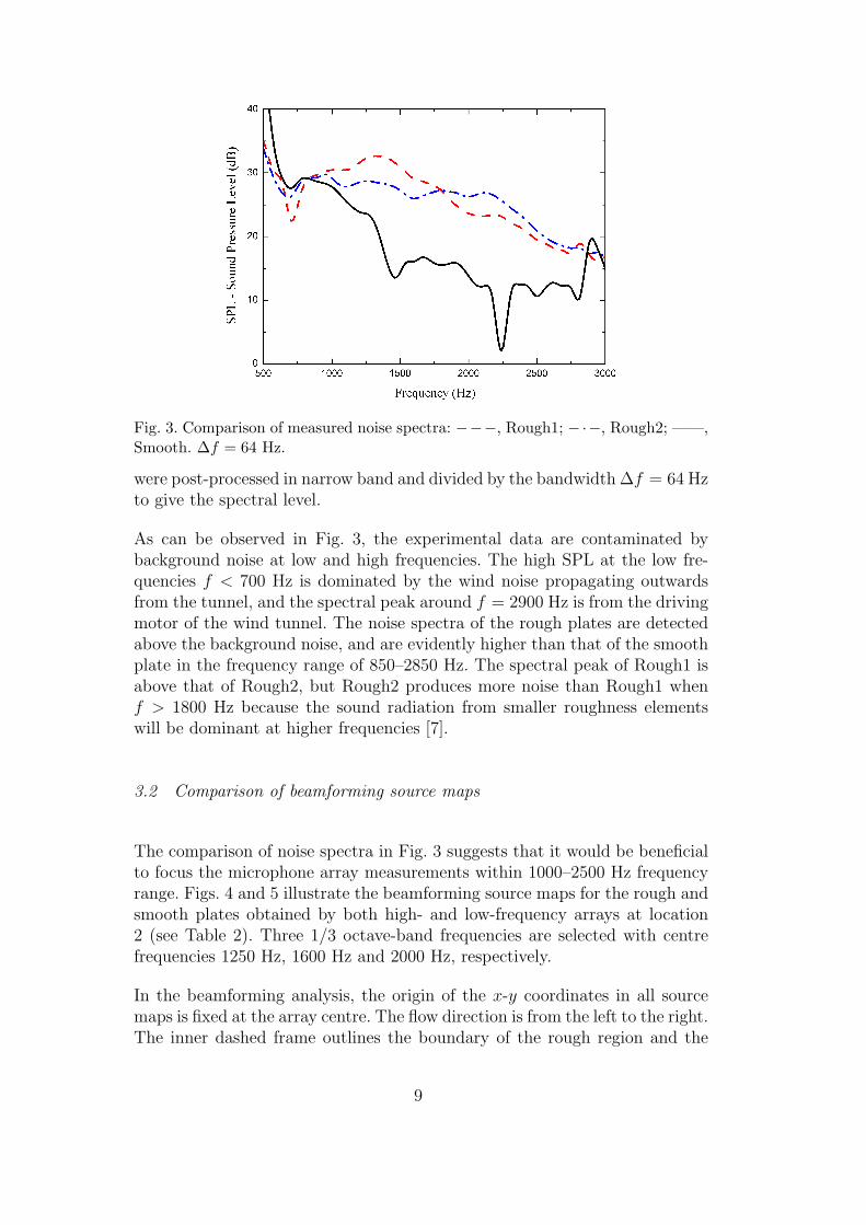
Fig. 3. Comparison of measured noise spectra: −−−, Rough1; −·−, Rough2; ——,Smooth. ∆f = 64 Hz.

were post-processed in narrow band and divided by the bandwidth ∆f = 64 Hzto give the spectral level.

As can be observed in Fig. 3, the experimental data are contaminated bybackground noise at low and high frequencies. The high SPL at the low fre-quencies f < 700 Hz is dominated by the wind noise propagating outwardsfrom the tunnel, and the spectral peak around f = 2900 Hz is from the drivingmotor of the wind tunnel. The noise spectra of the rough plates are detectedabove the background noise, and are evidently higher than that of the smoothplate in the frequency range of 850–2850 Hz. The spectral peak of Rough1 isabove that of Rough2, but Rough2 produces more noise than Rough1 whenf > 1800 Hz because the sound radiation from smaller roughness elementswill be dominant at higher frequencies [7].

3.2 Comparison of beamforming source maps

The comparison of noise spectra in Fig. 3 suggests that it would be beneficialto focus the microphone array measurements within 1000–2500 Hz frequencyrange. Figs. 4 and 5 illustrate the beamforming source maps for the rough andsmooth plates obtained by both high- and low-frequency arrays at location2 (see Table 2). Three 1/3 octave-band frequencies are selected with centrefrequencies 1250 Hz, 1600 Hz and 2000 Hz, respectively.

In the beamforming analysis, the origin of the x-y coordinates in all sourcemaps is fixed at the array centre. The flow direction is from the left to the right.The inner dashed frame outlines the boundary of the rough region and the

9

Fig. 4. Comparison of beamforming source maps: (a) Rough1; (b) Rough2; (c)Smooth. High-frequency microphone array.

dashdotted line downstream denotes the trailing edge. Note that in the currentsetup, only two rough panels were mounted into the 0.64× 0.64 m2 recess toform a smaller rough region upstream, which helps reduce the interference ofsound scattering from the trailing edge. In addition, the source powers havebeen converted to SPL data at a reference distance of 1/

√4π m from the

source [17]. The grey-scale bar gives the SPL in dB, and the grey-scale barsfor the rough and smooth plates at the same frequency are shown on identicalscales for easy comparison. The dynamic ranges of the source maps obtainedby the high- and low-frequency arrays are about 12 dB and 16 dB, respectively.

As shown in Figs. 4 and 5, the source strengths on the rough plates exceedthose on the smooth plate by about 10–15 dB. The source patterns of the tworough plates appear very similar with higher SPL for Rough1 at frequencies of1250 and 1600 Hz. However at f = 2000 Hz, the source strengths of Rough2exceed those of Rough1, which is consistent with the noise spectra data inFig. 3. The major lobe of maximum source strengths occurs in the upstreamportion of the rough region. This is because the ratio of roughness height toboundary-layer thickness, R/δ, decreases as the boundary layer grows alongthe plate chord, which makes the downstream roughness elements less signifi-cant as sound scatterers.

10

Fig. 5. Comparison of beamforming source maps: (a) Rough1; (b) Rough2; (c)Smooth. Low-frequency microphone array.

Comparing the source maps in Figs. 4 and 5, we find that the low-frequencyarray gives better resolution than the high-frequency array due to the se-lected low frequencies and the widely distributed sources in this case. Thelow-frequency array is able to detect a secondary lobe around the light dash-dotted line, as can be seen in Fig. 5, which is principally produced by thetrailing edge. The rough plates also generate stronger trailing-edge noise thanthe smooth plate, as predicted by Liu and Dowling [7], because on a roughplate the friction velocity uτ and boundary-layer thickness δ are increased dueto the enhanced surface drag and turbulence production [19].

However, we notice that the high-frequency array predicts 8–9 dB higher max-imum SPL than the low-frequency array at all frequencies. A possible expla-nation is that the beamforming algorithm assumes a monopole source withuniform directivity, and that the locations of the array microphones are differ-ent. The microphones of the high-frequency array are confined in a relativelysmall region where considerable sound radiation can be received from therough region upstream, while the microphones of the low-frequency array aredistributed in a much wider area and thus some of them are located closeto the z-axis where the roughness dipoles radiate little sound. The other andperhaps more important reason is based on the combination of the distributed

11

nature of roughness sources and the difference in the resolution of both arrays.The high-frequency array has poorer resolution than the low-frequency arrayat the chosen frequencies, and hence tends to capture more roughness sourcesand add up their source levels.

3.3 Effect of array locations

Table 2Locations of the array centre.

Location no. x (m) y (m) z (m)

1 0.04 0.025 0.47

2 0.18 0.025 0.64

3 0.36 0.025 0.60

The sound radiation from the two rough plates, Rough1 and Rough2, wasmeasured at three streamwise locations to detect some directivity features ofthe dipole sources. The coordinates of the array centre for locations 1–3 arelisted in Table 2 with the origin O at the centre of the rough region (seeFig. 8). In the x-direction, location 1 is very close to the origin O, location2 is a bit downstream, and location 3 is further downstream and behind therear edge of the rough region. Location 1 is also closest to the origin O in thez-direction. In these measurements, four rough panels were used and so therough region is doubled in area compared with that in Figs. 4 and 5.

Fig. 6 shows the beamforming source maps of Rough1 and Rough2 obtainedby the high-frequency array at locations 1–3, respectively. As can be seenfrom Fig. 6, location 1 produces a major lobe upstream with a secondary lobedownstream. The minimum source strength lies in the middle of the roughregion. This is very close to the centre of the array and occurs because thedipoles do not radiate sound in their normal plane. At the chosen frequencyf = 2000 Hz, the secondary lobe of Rough2 is stronger than that of Rough1and covers a larger area, which has been predicted by the noise spectra com-parison in Fig. 3. In contrast, only the distributed major lobe exists in thesource maps at downstream locations 2 and 3. Higher maximum strengths canbe observed as the array shifts downstream from location 1 to locations 2 and3. All these features agree with the directivity characteristics of a distributionof dipole sources in the flow direction.

Comparing the distributed area of the major lobe at locations 1–3, we no-tice that the beamforming resolution becomes gradually worse as the arraymoves farther from the origin O. However at the nearest location, least radi-ated roughness noise is received by the microphone array due to the dipole

12

Fig. 6. Comparison of beamforming source maps at locations 1–3: (a) Rough1; (b)Rough2. High-frequency microphone array. f = 2000 Hz.

directivity. Therefore, the compromise solution is to choose an array location abit downstream from the central rough region, and this explains why location2 was used for the measurements in §3.2.

4 Theory

Liu and Dowling [7] have given the power spectral density PR(ω) of the far-fieldradiated roughness noise spectrum in the form:

PR(ω) =Aσµ2

4r2

R4

δ∗4

U2c

c2Φ(ω)D(θ, φ). (1)

In the above expression, A is the area of the rough region, the roughness den-sity σ = NπR2 means the fractional area of the plane covered by roughnesselements, and N is the average number of roughness elements per unit area.µ = 1/(1+ 1

4σ) is not appreciably different from unity. The convection velocity

Uc ≈ 0.6U , and the displacement boundary-layer thickness δ∗ ≈ δ/8 for prac-tical purposes. Φ(ω) is the point pressure frequency spectrum approximatedby Ahn [20] for the frequency spectrum data in Blake [21]:

Φ(ω) =

(τ 2wδ∗

U

)2π8.28Sh∗0.8[

1 + 4.1Sh∗1.7 + 4.4× 10−4Sh∗5.9] , (2)

13

(a)

(b)

Fig. 7. Predicted SPL of PR(ω)/A with streamwise distance x1 for chosen frequen-cies: � 1250 Hz, • 1600 Hz, N 2000 Hz. (a) Rough1; (b) Rough2.

where τw = ρ0u2τ is the mean wall shear stress, uτ the friction velocity and

Sh∗ = ωδ∗/U the Strouhal number. D(θ, φ) is the directivity function:

D(θ, φ) = I1 cos2 θ + I2 sin2 θ sin2 φ, (3)

where I1 and I2 are infinite double integrals with respect to the wavenumbervector κ = (κ1, 0, κ3) (details to be found in Ref. [7]), and θ and φ are thedirectivity angles shown in Fig. 8 with

0 6 θ 6 π and |φ| 6 π/2. (4)

The prediction scheme in Eq. (1) is applied to calculate sound radiation from

14

different streamwise portions of the two rough plates in the experiments. Thetheoretical results are for the power spectral density PR(ω) from a unit rougharea to an observer at

θ = π/4, φ = 0 and r = 1/√

4π m. (5)

Figure 7 shows the predicted SPL of PR(ω)/A distributed over the two roughplates at 1250, 1600 and 2000 Hz frequencies. At the two higher frequencies,PR(ω)/A decreases with streamwise distance x1 from the front edge of roughregion. At 1250 Hz, there is a maximum x1 at 0.11 m for the plate Rough1and at 0.16 m for Rough2.

On a rough plate, as the boundary layer grows along the chord (x-axis), thelocal boundary-layer properties δ∗ and uτ are increasing and decreasing, re-spectively, both of which are determined by x1. The overall dependence ofPR(ω)/A on x1 at a particular frequency is principally due to the variationof Φ(ω). More detailed investigation of the terms shows that the variation ofΦ(ω) accounts for the maximum of PR(ω)/A. At a frequency of 1250 Hz, Φ(ω)has a maximum at x1 = 0.11 m for Rough1 and at x1 = 0.16 m for Rough2.At the higher frequencies Φ(ω) decreases across the entire rough regions.

5 Comparison of theory and experiment

5.1 Motivation of theoretical simulation

The comparison of beamforming source maps, as discussed in §3.2, demon-strates that the rough plates produce distinctly stronger noise sources thanthe smooth plate and enhance the trailing-edge noise somewhat. However,these “source” maps are not a true representation of the locations and rel-ative strengths of the roughness dipoles because the beamforming algorithmassumes a distribution of monopole sources, and hence can not be used directlyto validate the theoretical prediction.

Jordan et al. [16] has shown that the standard beamforming technique is inad-equate for both the source location and the measurement of a simple dipole,and that this is due to the assumption of monopole propagation in the calcula-tion of the phase weights used to steer the focus of the array. They developeda correction to the beamforming algorithm to account for the dipole propaga-tion characteristics, and applied it to array measurements for an aeroacousticdipole produced by a cylinder in a cross flow. The true source location andsource energy of the dipole was then retrieved in the resulting source mapafter applying this correction.

15

The technique of Jordan et al. [16], however, is not applicable in the caseof a distribution of dipoles because their directivities and hence the requiredcorrections vary over the source region, unlike the case of a single dipole. Wedo not have access to the source code for array analysis software to modifythe algorithm for a distribution of axial dipoles. Furthermore, in practice thesource mechanisms of a general aeroacoustic system could be very complex.There might be a combination of both monopole and dipole sources, andthe dipoles may have axial and spanwise components. Therefore it would bedifficult to implement a beamformer consistent with the hypothesized type ofsources.

Instead of altering the beamformer, an indirect approach is to theoreticallysimulate a distribution of incoherent dipoles over a rigid plate using the pre-diction scheme of Liu and Dowling [7], to process the predicted sound fieldthrough the same algorithm as the experiment, and to generate predictedsource maps that can be directly compared with the experimental results.This is equivalent to comparing theory and experiment after applying a filterwhich suppresses much the extraneous noise in the experiments. It provides anindirect way of comparing all the theoretical and experimental cross-powersbetween microphone pairs. For each grid point on the source-scanning plane,we determine the monopole source strength that gives the best fit to all thecross-powers. The quantitative agreement between the best-fit monopoles overthe source plane for the theoretical and experimental cross-powers validatesthe prediction scheme.

5.2 Simulation overview

The theoretical simulation for an experiment using phased microphone arraysis illustrated in Fig. 8. A program SIMSRC was utilized to describe a dis-tribution of incoherent dipoles over the rigid plate and simulate the sounddetected by the microphone array, as exactly in the experimental setup. Thisprogram requires the original source locations and source strengths as inputparameters. The post-processing and beamforming analysis of the simulationare based on a monopole source assumption as previously mentioned, and thusare not directly applicable to the dipole case of roughness noise. Nevertheless,SIMSRC is able to generate cross-power data for incoherent groups of coher-ent monopole sources [17]. In this case, each dipole source can be modeled bycoherent pairs of closely spaced monopoles with opposite phase. Because therigid plate behaves as a passive reflector, the mirror sources were also takeninto account as coherent with the original sources. The distribution of incoher-ent dipoles was therefore modeled by incoherent groups of the four coherentmonopole sets.

16

Fig. 8. Schematic of the theoretical simulation.

The phased microphone array is generally used to detect the source locationsand source patterns, and the SPL data shown in source maps are usuallyobtained as relative and just for reference. In this study, however, we at-tempted to simulate the real source strengths in magnitude as well as thesource locations. The simulated dipole sources were located at each hemi-spherical boss and the equivalent source strengths were determined from theprediction scheme of Liu and Dowling [7] as described below. The simulatedacoustic field was then processed in the same way as in the experiments toobtain predicted beamforming source maps.

We now commence the determination of equivalent source strengths with thederivation of the acoustic field of a dipole source. The mean flow effects havebeen neglected since the prediction scheme is based on an assumption of lowMach number which is also satisfied in the experimental setup (M < 0.1).The shear-layer refraction has therefore not been considered in the derivation,neither.

17

5.3 Acoustic field of a dipole

The acoustic frequency spectrum for an ideal monopole in a medium withoutflow can be expressed as [22]:

p(ω) =−a(ω)

4πre−ikr, (6)

where a(ω) is the monopole strength in frequency domain, k = ω/c is theacoustic wavenumber, and r is the propagation distance from source to ob-server.

A dipole source can be modeled as a coherent pair of closely placed monopoleswith opposite phase at a distance l apart, as shown in Fig. 8. The acousticfield of a dipole is obtained by combining the radiated sound of these twomonopoles:

p(ω) =−a(ω)

4πr+

e−ikr+ − −a(ω)

4πr−e−ikr− , (7)

where r+ and r− are the propagation distances for the two monopoles withopposite phase, r+ ≈ r + l

2cos θ,

r− ≈ r − l2cos θ.

(8)

In the far field, r � l, the amplitude difference between the radiated sound oftwo monopoles is small, and thus in Eq. (7) r+ and r− can be approximatedby r in the amplitude part. However, the phase difference can not be ignored.Substituting Eq. (8) into Eq. (7), we obtain

p(ω)≈ −a(ω)

4πre−ikr ·

(e−i kl cos θ

2 − ei kl cos θ2

)(9)

=−a(ω)

4πre−ikr ·

(−2i sin

kl cos θ

2

).

If the dipole is compact (i.e. kl � 1), Eq. (9) can be simplified as:

p(ω) =a(ω)

4πre−ikr · ikl cos θ. (10)

In the presence of a reflecting rigid plate, the mirror source of the dipole needto be included, and hence the aggregate acoustic field can be obtained bymultiplying Eq. (10) by 2. The power spectral density of the acoustic frequencyspectrum p(ω) is:

P (ω) = Λ(ω)

∣∣∣∣∣ ikl cos θ

2πre−ikr

∣∣∣∣∣2

, (11)

18

where Λ(ω) is the power spectral density of a(ω),

a(ω)a(ω′) = 2πΛ(ω)δ(ω + ω′). (12)

5.4 Equivalent source strengths

As is evident from Eq. (3), the first term I1 cos2 θ describes the sound fielddue to a dipole in the flow direction, while the second term I2 sin2 θ sin2 φaccounts for a dipole in the plate plane but normal to the flow direction. Tolink this to the beamforming simulation, we consider a distribution of dipoleswith two dipoles DPL1 and DPL2 at each hemispherical boss and determinethe equivalent source strengths a1(ω) and a2(ω). Herein DPL1 is orientated inthe flow direction and DPL2 is normal to the flow direction, respectively.

Now we consider a rough region of unit area which contains N roughnesselements. The acoustic field of DPL1 can be described by Eq. (11), and hencethe aggregate power spectral density of N incoherent dipoles is

P1(ω) =N∑

j=1

P1j(ω) =NΛ1(ω)k2l2 cos2 θ

4π2r2. (13)

From the prediction scheme (1), the contribution of the dipole DPL1 to PR(ω)for a unit rough area A = 1 is

PR1(ω) =σµ2

4r2

R4

δ∗4

U2c

c2Φ(ω)I1 cos2 θ. (14)

Combining Eqs. (13) and (14) gives the theoretical prediction for Λ1(ω):

Λ1(ω) =π2σµ2

Nl2R4

δ∗4

U2c

ω2Φ(ω)I1. (15)

The above derivation is based on the continuous Fourier transform (CFT)and Λ1(ω) denotes the power spectral density of a1(ω). However in the the-oretical simulation for acoustic measurements, the discrete Fourier transform(DFT) is applied and thus Λ1(ω) actually means the frequency-dependentsource power [22]. In this case, the equivalent source strength a1(ω) requiredby the simulation program SIMSRC can not be derived directly from Λ1(ω)in Eq. (15). Instead, it is necessary to compare the total source power in afrequency band between the CFT and DFT.

The predicted total power of Λ1(ω) in the frequency band [ω1, ωn] is

a21(t) =

1

2π

∫ ωn

ω1

Λ1(ω) dω. (16)

19

In the simulation, the total power of Λ1(ω) in [ω1, ωn] can be expressed as [23]:

Λ1tot =n∑

i=1

|a1(ωi)|2 = n|a1(ω)|2, (17)

where n is the number of frequency intervals; a1(ωi) is the equivalent sourcestrength in the ith frequency interval; a1(ω) is the average source strengthof n intervals, ω1, ω2, . . . , ωn, and is used as the input source strength for thefrequency band [ω1, ωn] in SIMSRC. By equating the total source powers in theprediction (16) and simulation (17), the predicted equivalent source strengthfor the two coherent monopoles of DPL1 is given by

|a1(ω)| = µUc

l

R2

δ∗2

[πσI1

2Nn

∫ ωn

ω1

Φ(ω)

ω2dω

]1/2

. (18)

Just as the power spectral density PR(ω), the equivalent source strength a1(ω)decreases with increasing streamwise position along the rough region, except atthe lowest frequency f = 1250 Hz where it has a maximum near x1 = 0.11 mfor the plate Rough1 and 0.16 m for Rough2. Equation (18) describes thevariation of the roughness dipole strength with streamwise locations. The valueof the dipole size l is unimportant because Λ1(ω) ∼ l−2 from Eq. (15) andhence the predicted power spectral density P1(ω) is independent of l. Theonly constraint is that l should satisfy the compact dipole assumption kl � 1.In the present study l = R is used.

Similarly, the theoretical prediction for |a2(ω)| can be obtained as:

|a2(ω)| = µUc

l

R2

δ∗2

[πσI2

2Nn

∫ ωn

ω1

Φ(ω)

ω2dω

]1/2

. (19)

Nevertheless, the contribution of I1 to PR(ω) is more important than thatof I2 for sufficiently large roughness elements [7], i.e. the roughness Reynoldsnumber

Reτ = Ruτ/ν > 1000, (20)

where ν is the kinematic viscosity. In addition, in Fig. 8 the centre of themicrophone array is located very close to the centre of the rough region in they-direction which is the direction of the dipole DPL2. This results in a nearlynegligible contribution of DPL2 to the SPL of the source maps as there is nosound radiation in the normal plane of the DPL2 orientation. The predicted|a1(ω)| and |a2(ω)| from Eqs. (18) and (19) were then used in the theoreticalsimulation as the equivalent source strengths for DPL1 and DPL2, respectively.

20

5.5 Results

To compare the source maps of measured roughness noise and simulated dipolesources, “clean” source maps of Rough1 and Rough2 need to be obtained.Although the reverberation noise of a closed-return wind tunnel is avoidedin the case of out-of-flow measurements in an open jet, Figs. 4 and 5 stillindicate considerable contamination from other sound sources, e.g. trailingedge, leading edge, seams. A straightforward but effective method to eliminatethe contamination is to subtract the source powers of the smooth plate fromthose of the rough plates. This method was applied to the raw source maps inFigs. 4 and 5, and corrected “clean” source maps were obtained for comparisonwith simulation.

Figs. 9–12 illustrate the comparison of measured and simulated source mapsfor Rough1 and Rough2, and both the high- and low-frequency array data areshown. Unlike the identical grey-scale bars for Rough1, Rough2 and Smooth inFigs. 4 and 5, the grey-scale bars in Figs. 9–12 gives the unaltered maximumsource strengths for a better comparison of measurement and simulation. Thesimulated equivalent source strengths at each 1/3 octave band frequency havebeen averaged over the whole bandwidth, as in the beamforming analysis ofthe experimental data.

In all these figures, the top row shows the “clean” source maps based on theexperimental data with the Smooth source powers subtracted. As can be seenfrom the high-frequency array data in Figs. 9 and 11, the SPL of the “clean”source maps has been diminished a bit and the major lobe is concentratedmore in the upstream rough region compared with the raw source maps inFig. 4. This correction is shown more evidently for the low-frequency arraydata in Figs. 10 and 12 in which the interference from the trailing-edge noiseseen originally in Fig. 5 has been greatly reduced.

The bottom row of Figs. 9–12 shows the corresponding source maps by simu-lating a distribution of incoherent dipoles over the rigid plate with strengthsderived using the model of Liu and Dowling [7]. The beamforming predictionsof the source patterns of measurement and simulation exhibit satisfactorysimilarities, which confirms the dipole nature of surface roughness noise. Themajor lobe in the top row gradually reduces in the spanwise direction (y-axis)along the plate chord (x-axis), whereas in the bottom row the major lobealmost fills the entire dashed frame. This is because in the experiment theboundary of the open jet expands along the flow direction as the jet mixeswith the still air in free space. The expansion effect results in a decrease offlow velocity around the jet boundary. In the simulation, however, this effect istoo complicated to be considered for the correction of the predicted equivalentsource strengths around the jet boundary.

21

Fig. 9. Comparison of beamforming source maps for Rough1: (a) measurement(“clean”); (b) simulation. High-frequency microphone array.

Fig. 10. Comparison of beamforming source maps for Rough1: (a) measurement(“clean”); (b) simulation. Low-frequency microphone array.

Furthermore, as indicated by the grey-scale bars of Figs. 9–12, the simulationprogram SIMSRC is capable of approximately predicting the equivalent sourcestrengths of roughness noise in magnitude at 1250 and 1600 Hz frequencies,which provides further form of validation for Liu and Dowling’s predictionscheme [7] from the perspective of microphone array measurements. However,a discrepancy of about 3 dB can be observed for the comparison at 2000 Hz,and this should be ascribed to the limitation of Liu and Dowling’s predictionscheme which predicted spectral levels a few dB higher than the measured

22

Fig. 11. Comparison of beamforming source maps for Rough2: (a) measurement(“clean”); (b) simulation. High-frequency microphone array.

Fig. 12. Comparison of beamforming source maps for Rough2: (a) measurement(“clean”); (b) simulation. Low-frequency microphone array.

roughness noise in f > 1.7 kHz frequency [7]. In addition, SIMSRC predictssomewhat higher source strengths in the downstream portion of the roughregion, namely, the streamwise gradient of simulated source strengths are abit lower than that of the measured source strengths. Hence there is scope toimprove the theoretical model to capture these aspects of surface roughnessgenerated noise.

23

6 Concluding remarks

Howe [1] has presented a theoretical model of sound generation by turbulentboundary-layer flow over a rough wall. The dipole-type roughness noise wasattributed to the scattering of the turbulence near-field into radiated sound atsmall surface irregularities. Liu and Dowling [7] then extended Howe’s modelfor numerically quantifying the far-field radiated roughness noise, and haveobtained reasonable agreement between measurement and prediction in rough-ness noise spectral levels.

In this paper, phased microphone arrays have been applied to the measure-ment and simulation of surface roughness noise. From the resulting beamform-ing source maps, the rough plates exhibited higher source strengths than thesmooth plate, and the trailing-edge noise was somewhat enhanced by surfaceroughness. Measurements at three streamwise locations demonstrated somefeatures of the dipole directivity.

Theoretical simulations have been performed for a distribution of incoherentdipoles over the rough plates with the equivalent source strengths determinedby Liu and Dowling’s prediction scheme [7]. The same beamfroming algorithmwas applied to measurement and simulation and the source maps exhibitedsatisfactory similarities in source pattern with approximate source strengths.This has confirmed the dipole nature of roughness noise and validated thesource amplitude predicted by Liu and Dowling [7]. However, the streamwisegradient of the source strengths was a bit underestimated in the simulations,and at the highest frequency the source strengths were overestimated by about3 dB, which indicates that there is scope for an improved theoretical predictionwhich captures these aspects of surface roughness noise.

As well as a contribution to surface roughness noise, the proposed process-ing technique has wider applicability. For many airframe applications, theaeroacoustic sources arise from dipoles and quadrupoles. In this case, arraymeasurements can be misinterpreted due to the monopole assumption in thestandard beamforming algorithm. We analyzed the theoretical model throughthe array simulation software so that indirect comparison between theory andexperiment can be made for the dipole-type surface roughness noise. It is rec-ommended that further investigations be conducted to apply this techniqueto more complex systems, for example, quadrupole-type jet noise.

24

Acknowledgements

This work is supported in part by Silent Aircraft Initiative (SAI), a collabo-rative project funded by the Cambridge-MIT Institute. The design and man-ufacture of the microphone array system was assisted by National AerospaceLaboratory (NLR), The Netherlands. The authors would like to thank Dr.Pieter Sijtsma of NLR for the technical support to the results obtained fromthe microphone arrays. Y. Liu acknowledges the financial support providedby the Overseas Research Students (ORS) Awards Scheme and the GatesCambridge Scholarships.

References

[1] M. S. Howe, On the generation of sound by turbulent boundary layer flow overa rough wall, Proceedings of the Royal Society of London A395 (1984) 247–263.

[2] M. S. Howe, The influence of viscous surface stress on the production of soundby a turbulent boundary layer over a rough wall, Journal of Sound and Vibration104 (1) (1986) 29–39.

[3] M. S. Howe, The turbulent boundary-layer rough-wall pressure spectrum atacoustic and subconvective wavenumbers, Proceedings of the Royal Society ofLondon A415 (1988) 141–161.

[4] M. S. Howe, Surface pressures and sound by turbulent flow over smooth andrough walls, Journal of the Acoustical Society of America 90 (2) (1991) 1041–1047.

[5] M. S. Howe, Acoustics of Fluid-Structure Interactions, Cambridge UniversityPress, Cambridge, UK, 1998.

[6] A. S. Hersh, Surface roughness generated flow noise, No. 83-0786, AIAA Paper,1983.

[7] Y. Liu, A. P. Dowling, Assessment of the contribution of surface roughness toairframe noise, AIAA Journal 45 (4) (2007) 855–869.

[8] G. M. Corcos, The structure of the turbulent pressure field in boundary- layerflows, Journal of Fluid Mechanics 18 (3) (1964) 353–378.

[9] B. M. Efimtsov, Characteristics of the field of turbulent wall pressurefluctuations at large reynolds numbers, Soviet Physics Acoustics 28 (4) (1982)289–292.

[10] A. V. Smol’yakov, V. M. Tkachenko, Model of a field of pseudosonic turbulentwall pressures and experimental data, Soviet Physics Acoustics 37 (6) (1991)627–631.

25

[11] D. M. Chase, Modeling the wavevector-frequency spectrum of turbulentboundary layer wall pressure, Journal of Sound and Vibration 70 (1) (1980)29–67.

[12] D. M. Chase, The character of the turbulent wall pressure spectrum atsubconvective wavenumbers and a suggested comprehensive model, Journal ofSound and Vibration 112 (1) (1987) 125–147.

[13] J. Billingsley, R. Kinns, The acoustic telescope, Journal of Sound and Vibration48 (4) (1976) 485–510.

[14] D. H. Johnson, D. E. Dudgeon, Array Signal Processing: Concepts andTechniques, Prentice Hall, London, 1993.

[15] R. P. Dougherty, Beamforming in Acoustic Testing, Published in “AeroacousticMeasurements”, Edited by T. J. Mueller, Springer-Verlag, Berlin, 2002.

[16] P. Jordan, J. A. Fitzpatrick, J.-C. Valiere, Measurement of an aeroacousticdipole using a linear microphone array, Journal of the Acoustical Society ofAmerica 111 (3) (2002) 1267–1273.

[17] P. Sijtsma, Experimental Techniques for Identification and Characterisation ofNoise Sources, Published in “Advances in Aeroacoustics and Applications”, VKILecture Series 2004-05, Edited by J. Anthoine and A. Hirschberg, 2004.

[18] R. K. Amiet, Refraction of sound by a shear layer, Journal of Sound andVibration 58 (2) (1978) 467–482.

[19] H. Schlichting, Boundary Layer Theory, seventh Edition, McGraw-Hill, NewYork, 1979.

[20] B. Ahn, Modeling unsteady wall pressures beneath turbulent boundary layers,Ph.D. thesis, Department of Engineering, University of Cambridge, Cambridge,UK (2005).

[21] W. K. Blake, Turbulent bounday-layer wall-pressure fluctuations on smoothand rough walls, Journal of Fluid Mechanics 44 (4) (1970) 637–660.

[22] A. P. Dowling, J. E. Ffowcs Williams, Sound and Sources of Sound, EllisHorwood, Chichester, UK, 1983.

[23] N. C. Geckinli, D. Yavuz, Discrete Fourier Transformation and Its Applicationsto Power Spectra Estimation, Published in “Studies in Electrical and ElectronicEngineering 8”, Elsevier, New York, 1983.

26